Benchmarking discrete truncated Wigner approximation and restricted Boltzmann neural networks with the exact dynamics of a Rydberg atomic chain

Abstract

We benchmark the discrete truncated Wigner approximation (DTWA) and artificial neural networks (ANN) of restricted Boltzmann machine methods with the exact excitation and correlation dynamics in a chain of ten Rydberg atoms. The initial state is where all atoms are in their electronic ground state. We characterize the excitation dynamics using the maximum and average number of Rydberg excitations. DTWA and ANN are reliable for sufficiently small Rydberg-Rydberg interactions but fail at large interaction strengths to capture the excitation dynamics. Concerning the correlations, ANN looks more promising among the two methods as the second-order bipartite and average two-site Rényi entropies are captured accurately when the Rydberg-Rydberg interactions are small. The second-order DTWA can accurately quantify the correlations for initial periods for small interaction strengths but fail for large interactions.

1 Introduction

In general, analyzing the dynamics of a quantum many-body system is a formidable task because of the exponentially large Hilbert space. Further, strong quantum correlations or entanglement growth makes quantum dynamics more intriguing. Developing numerical approaches accurately capturing quantum correlations has been a main focus in the recent past [1]. It led to the development of various numerical techniques based on tensor network states and phase-space methods. The former includes, for instance, density-matrix renormalization group (DMRG) (for both ground states and dynamics) [2, 3, 4, 5, 6, 7] in which the Hilbert space is truncated to states with significant probabilities, leading to a polynomial growth in Hilbert space with system size. DMRG is an excellent tool for studying one-dimensional systems with weak entanglement. The phase-space methods are semi-classical and involve solving classical equations of motion for the phase-space variables. Examples are the truncated Wigner approximation (TWA) [8, 9] and its discrete version (DTWA) [10, 11, 12]. DTWA was initially developed for spin-1/2 systems and later generalized to higher spin [13], higher dimensional phase space [14], and dissipative systems [15]. DTWA is also employed to study dynamical phase transitions in large spin systems [16]. The results from DTWA have shown good agreement with a few experiments involving Rydberg [17, 18, 19, 20] and dipolar atoms [21, 22, 23] where the system is described by an XY model. Generally, such an agreement is only sometimes guaranteed and is limited to a few cycles of the dynamics, depending on the strength and range of inter-particle interactions [24].

At the same time, there is a growing interest in using machine learning methods to study physics problems [25, 26]. Artificial neural networks (ANN) are proposed to explore quantum many-body systems in which the quantum states are represented by restricted-Boltzmann-machine (RBM) type network architecture with complex weights [27, 28, 29, 30, 31, 32]. Due to its design, RBM is naturally suited for spin-1/2 systems. The RBM ansatz has shown good agreement with ground state calculations. Whereas for dynamics, the agreement is limited again for short periods [28, 29, 30].

On the other side, quantum simulators based on ultra-cold Rydberg atoms have shown tremendous progress, extending to large system sizes beyond a regime where classical computers can tackle [33, 34, 36, 37, 38, 39, 40, 35, 41, 42]. Hence, it becomes necessary to develop or test advanced numerical approaches to cross-verify the dynamics of atomic lattices with Rydberg excitations. Rydberg atoms are known to exhibit prodigious interactions [43, 44] leading to the phenomenon of the Rydberg, or dipole blockade [45, 46, 47]. Blockade and anti-blockade can lead to strong correlation effects, which can simulate non-trivial phases in condensed-matter [34, 48, 49, 50, 51, 52, 53, 54, 55] and find applications in quantum information protocols [43, 56, 57, 58, 59, 60, 61]. Typically, the Rydberg atomic setup has been modeled as a gas of interacting two-level atoms, with either dipolar or van der Waals-type interactions [63]. Further, making the atom-light couplings time-dependent provides fine-tuning in quantum state preparation and expands the territory of problems that can be addressed [42, 62, 64, 65, 66].

In this work, we numerically analyze the excitation and correlation dynamics in a chain of ten atoms where each atom is initially in its ground state, which is coupled to a Rydberg state by a light field. In particular, we explore the oscillatory behavior of the number of excitations, the dependence of the maximum and the average number of excitations on the interaction strengths, and finally, the dynamics of bipartite and mean two-site second-order Rényi entropy. The maximum number of excitations is always seen during the first oscillation cycle, and at large interaction strengths, the Rydberg blockade suppresses the excitation fraction leading to a saturation in average and maximum number of excitations. The collapse and revival in the number of excitations for sufficiently small interactions are also discussed.

Our work primarily aims to compare the exact results with that of DTWA and ANN (RBM network) and show how well the latter methods can capture the dynamics of one-dimensional Rydberg lattice gases. Using DTWA, we obtain results with and without adding the second-order correlations from the BBGKY hierarchy, which we term first and second-order DTWA. DTWA and ANN accurately capture the excitation dynamics over significant periods for small interaction strengths. However, both methods fail to replicate the revival of populations, which occurs at longer times. As interaction strengths increase, both methods show agreement only for shorter periods. However, ANN is more reliable for more significant interactions, especially when computing the average and maximum number of excitations. In addition, the second-order DTWA suffers from numerical instabilities for considerable interaction strengths, which is also reported in the study of quantum spin models [24]. bipartite and mean two-site second-order Rényi entropy

The paper is structured as follows. In section 2, we introduce the physical setup and the governing Hamiltonian. In sections 3 and 4, we details of the DTWA and ANN techniques are provided. The excitation and correlation dynamics are shown in sections 5 and 6, respectively. Finally, we provide conclusions and outlook in section 7.

2 Setup and Model

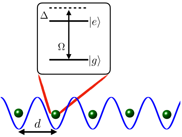
Figure 1: The schematic diagram of the setup consists of an array of atoms with a spacing of $d$. For each atom, the ground state $|g\rangle$ is coupled to a Rydberg state $|e\rangle$ with a light field with a detuning $\Delta$ and Rabi frequency $\Omega$.

We consider a chain of atoms with lattice spacing $d$ as shown in Figure 1. The electronic ground state $|g\rangle$ of each atom is coupled to a Rydberg state $|e\rangle$ with a detuning $\Delta$ and a Rabi frequency $\Omega$. In the frozen gas limit, the system is described by the Hamiltonian ($\hbar=1$):

$$\hat{H}(t)=-\Delta\sum_{i=1}^{N}\hat{\sigma}_{ee}^{i}+\frac{\Omega}{2}\sum_{i=1}^{N}\hat{\sigma}_{x}^{i}+\sum_{i<j}V_{ij}\hat{\sigma}_{ee}^{i}\hat{\sigma}_{ee}^{j},$$ (1)

where $\hat{\sigma}_{ab}=|a\rangle\langle b|$ with $a,b\in\{e,g\}$ includes both transition and projection operators, and $\hat{\sigma}_{x}=\hat{\sigma}_{eg}+\hat{\sigma}_{ge}$. We assume the Rydberg excited atoms interact via van der Waals potential $V_{ij}=C_{6}/r_{ij}^{6}$ [44], where $C_{6}$ is the interaction coefficient, and $r_{ij}$ is the separation between $i$th and $j$th Rydberg excitations. The exact dynamics of the system is analyzed by solving the Schrödinger equation: $i\partial\psi(t)/\partial t=\hat{H}(t)\psi(t)$.

Introducing $\hat{\sigma}_{ee}^{i}=(1+\hat{\sigma}_{z}^{i})/2$, we rewrite the Hamiltonian as, $\hat{H}=\sum_{i}\hat{H}_{i}+\sum_{i<j}\hat{H}_{ij}$, where $\hat{H}_{i}=-\Delta^{{\rm eff}}_{i}\hat{\sigma}_{z}^{i}+\Omega\hat{\sigma}_{x}^{i}/2$ consists of single particle terms with an effective detuning $\Delta^{{\rm eff}}_{i}=\Delta-\sum_{j\neq i}V_{ij}/2$, and $\hat{H}_{ij}=V_{ij}\hat{\sigma}_{z}^{i}\hat{\sigma}_{z}^{j}/4$ contains the two-body interactions. Henceforth, we take $\Delta=0$. The model is nothing but a quantum Ising model with an additional longitudinal field and long-range Ising interactions. We characterize the dynamics via experimentally relevant quantities such as the instantaneous number of excitations $N_{e}(t)=\sum_{i}\langle\psi(t)|\hat{\sigma}_{ee}^{i}|\psi(t)\rangle$, the maximum $N_{e}^{max}$ and the average number of excitations $N_{e}^{avg}=(1/T)\int_{0}^{T}N_{e}(t)$ over a period of time $T$. Later in section 6, we analyze bipartite and mean two-site second-order Rényi entropy of the corresponding dynamics.

3 Discrete truncated Wigner approximation: Equations of motion

Here, we briefly outline the method of DTWA. Each atom forms a two-level system (equivalently a qubit or a spin-1/2 particle) composed of the ground state $|g\rangle$ and Rydberg state $|e\rangle$. The finite and discrete Hilbert space is mapped onto a discrete quantum phase-space via the Wigner-Weyl transform. A single qubit discrete phase-space is defined as a real-valued finite field spanned by four-phase points, denoted by $\alpha\equiv(m,n)\in\{(0,0),(0,1),(1,0),(1,1)\}$ [67, 68, 10]. For each $\alpha$, one can associate a phase-point operator $\hat{A}_{\alpha}=(\mathcal{I}+{\bf r}_{\alpha}\cdot\hat{\bf\sigma})/2$, where $\mathcal{I}$ is the identity operator and $\hat{\bf\sigma}=(\hat{\sigma}_{x},\hat{\sigma}_{y},\hat{\sigma}_{z})$ are the Pauli matrices. The three-vectors $\{{\bf r}_{\alpha}\}$ do not have a unique choice, and the best suitable sampling scheme for a given Hamiltonian can be appropriately selected [12]. For the initial state we take, the best results are obtained using ${\bf r}_{(1,0)}=(1,0,-1)$, ${\bf r}_{(1,1)}=(-1,0,-1)$, ${\bf r^{\prime}}_{(1,0)}=(0,1,-1)$ and ${\bf r^{\prime}}_{(1,1)}=(0,-1,-1)$, which is kept throughout.

Any observable $\hat{\mathcal{O}}$ from the Hilbert space is mapped into a Weyl symbol $\mathcal{O}^{W}_{\alpha}=\Tr(\hat{\mathcal{O}}\hat{A}_{\alpha})/2$ in the discrete phase-space. The density operator $\hat{\rho}$ is written as $\hat{\rho}=\sum_{\alpha}w_{\alpha}\hat{A}_{\alpha}$, where the weights $w_{\alpha}=\Tr(\hat{\rho}\hat{A}_{\alpha})/2$ form a quasi-probability distribution similar to the original Wigner function and is the Weyl symbol of the density matrix. $w_{\alpha}$ can also take negative values. For a system of $N$ two-level atoms, we have a discrete phase-space of $4^{N}$ points denoted simply by $\vec{\alpha}=\{\alpha_{1},\alpha_{2},...,\alpha_{N}\}$. Let the initial density matrix be,

$$\hat{\rho}_{0}=\sum_{\vec{\alpha}}W_{\vec{\alpha}}\ \hat{A}_{\alpha_{1}}\otimes\hat{A}_{\alpha_{2}}\otimes...\otimes\hat{A}_{\alpha_{N}},$$ (2)

which corresponds to a product state with $W_{\vec{\alpha}}=w_{\alpha_{1}}w_{\alpha_{2}}...w_{\alpha_{N}}$ and $\sum_{\vec{\alpha}}=\sum_{\alpha_{1},\alpha_{2},...}$. The density matrix at time $t$ is defined as

$$\hat{\rho}(t)=\sum_{\vec{\alpha}}W_{\vec{\alpha}}\ \hat{\mathcal{A}}^{\vec{\alpha}}_{1...N}(t),$$ (3)

with

$$\hat{\mathcal{A}}^{\vec{\alpha}}_{1...N}(t)=\hat{U}(t)\hat{A}_{\alpha_{1}}\otimes\hat{A}_{\alpha_{2}}\otimes.....\otimes\hat{A}_{\alpha_{N}}\hat{U}^{\dagger}(t)$$ (4)

where $\hat{U}(t)=\exp(-i\hat{H}t)$ is the unitary time evolution operator. Here, we do not consider all the trajectories but a random sample of $N_{s}$ number of trajectories out of $4^{N}$ trajectories, and hence the density matrix is defined as,

$$\hat{\rho}(t)=\sum_{\alpha}\frac{1}{N_{s}}\hat{\mathcal{A}}^{\vec{\alpha}}_{1...N}(t).$$ (5)

The operator $\hat{\mathcal{A}}^{\vec{\alpha}}_{1...N}(t)$ satisfies the Liouville-von Neumann equation [12]:

$$i\frac{\partial}{\partial t}\hat{\mathcal{A}}^{\vec{\alpha}}_{1...N}=\left[\hat{H},\hat{\mathcal{A}}^{\vec{\alpha}}_{1...N}\right]$$ (6)

We can treat the operator $\hat{\mathcal{A}}^{\vec{\alpha}}_{1...N}$ as a quasi-density-matrix since its trace is equal to one, but need not be a positive definite. The reduced $\hat{\mathcal{A}}$ operators are obtained by tracing out remaining parts of the system as,

$$\hat{\mathcal{A}}^{\vec{\alpha}}_{i}=\mathrm{Tr}_{\cancel{i}}\hat{\mathcal{A}}^{\vec{\alpha}}_{1...N},\ \ \ \ \ \ \ \ \ \ \ \ \ \ \hat{\mathcal{A}}^{\vec{\alpha}}_{ij}=\mathrm{Tr}_{\cancel{i}\cancel{j}}\hat{\mathcal{A}}^{\vec{\alpha}}_{1...N}\$$ (7)

where $\mathrm{Tr}_{\cancel{i}}$ denotes a partical trace over all the indices except $i$ and similarly for $\mathrm{Tr}_{\cancel{i}\cancel{j}}$ with $i\neq j$. For reduced density operators, using the Liouville-von Neumann equation, one can write down the hierarchy of equations of motions, so-called the BBGKY hierarchy. Following the same prescription, a similar hierarchy of equations of motions for the reduced $\hat{\mathcal{A}}$ operators is obtained, by introducing the cluster expansion [12],

$$\hat{\mathcal{A}}_{ij} =\hat{\mathcal{A}}_{i}\hat{\mathcal{A}}_{j}+\hat{\mathcal{C}}_{ij}$$ (8)

$$\hat{\mathcal{A}}_{ijk} =\hat{\mathcal{A}}_{i}\hat{\mathcal{A}}_{j}\hat{\mathcal{A}}_{k}+\hat{\mathcal{A}}_{i}\hat{\mathcal{C}}_{jk}+\hat{\mathcal{A}}_{j}\hat{\mathcal{C}}_{ik}+....+\hat{\mathcal{C}}_{ijk}$$ (9)

$$\hat{\mathcal{A}}_{ijkl} =\hat{\mathcal{A}}_{i}\hat{\mathcal{A}}_{j}\hat{\mathcal{A}}_{k}\hat{\mathcal{A}}_{l}+\hat{\mathcal{A}}_{i}\hat{\mathcal{A}}_{j}\hat{\mathcal{C}}_{kl}+...+\hat{\mathcal{C}}_{ij}\hat{\mathcal{C}}_{kl}+...+\hat{\mathcal{C}}_{ijk}\hat{\mathcal{A}}_{l}+....+\hat{\mathcal{C}}_{ijkl},$$ (10)

where $\hat{\mathcal{A}}_{1},\hat{\mathcal{A}}_{2},...,\hat{\mathcal{A}}_{N}$ are the uncorrelated parts of $\hat{\mathcal{A}}_{1...N}$, and $\hat{\mathcal{C}}_{ij},\hat{\mathcal{C}}_{ijk}...$ operators incorporate the correlations between the particles arising from the inter-particle interactions. Note that, we have removed the superscript $\vec{\alpha}$ in $\hat{\mathcal{A}}_{j}$ for simplicity. Truncating beyond two-particle correlations, one obtains the first two equations of the BBGKY hierarchy as:

$$i\frac{\partial}{\partial t}\hat{\mathcal{A}}_{i} = [\hat{H}_{i},\hat{\mathcal{A}}_{i}]+\sum_{k\neq i}\mathrm{Tr}[\hat{H}_{ik},\hat{\mathcal{C}}_{ik}+\hat{\mathcal{A}}_{i}\hat{\mathcal{A}}_{k}]$$ (11)

$$i\frac{\partial}{\partial t}\hat{\mathcal{C}}_{ij} = [\hat{H}_{i}+\hat{H}_{j}+\hat{H}^{\mathrm{H}}_{i\cancel{j}}+\hat{H}^{\mathrm{H}}_{j\cancel{i}},\hat{\mathcal{C}}_{ij}]+[\hat{H}_{ij},\hat{\mathcal{C}}_{ij}+\hat{\mathcal{A}}_{i}\hat{\mathcal{A}}_{j}]+$$ (12)

$$\sum_{k\neq i,j}\left(\mathrm{Tr}_{k}[\hat{H}_{ik},\hat{A}_{i}\hat{\mathcal{C}}_{jk}]+\mathrm{Tr}_{k}[\hat{H}_{jk},\hat{\mathcal{A}}_{j}\hat{\mathcal{C}}_{jk}]\right)-$$

$$\hat{\mathcal{A}}_{i}\mathrm{Tr}_{i}[\hat{H}_{ij},\hat{\mathcal{C}}_{ij}+\hat{\mathcal{A}}_{i}\hat{\mathcal{A}}_{j}]-\hat{\mathcal{A}}_{j}\mathrm{Tr}_{j}[\hat{H}_{ij},\hat{\mathcal{C}}_{ij}+\hat{\mathcal{A}}_{i}\hat{\mathcal{A}}_{j}]$$

where $\hat{H}^{\mathrm{H}}_{i\cancel{j}}$ is a Hartree operator or Mean-field operator given by:

$$\hat{H}^{\mathrm{H}}_{i\cancel{j}}=\sum_{k\neq i,j}\mathrm{Tr}_{k}(\hat{H}_{ik}\hat{\mathcal{A}}_{k}).$$ (13)

At this point, one expands $\mathcal{A}$ and $\mathcal{C}$ operators in the basis of Pauli spin matrices,

$$\hat{\mathcal{A}}_{i} =\frac{1}{2}(\mathcal{I}+\hat{a}_{i}\cdot\hat{\sigma})$$ (14)

$$\hat{\mathcal{C}}_{ij} =\frac{1}{4}\sum_{\mu,\nu\in\{x,y,z\}}c^{\mu\nu}_{ij}\hat{\sigma}_{\mu}^{i}\hat{\sigma}_{\nu}^{j},$$ (15)

for $i\neq j$. Finally, one obtains the equation of motion for $a_{i}^{\mu}$ as,

$$\frac{1}{2}\dot{a}^{\mu}_{i} = \sum_{\gamma}\left[\frac{\Omega}{2}a^{\gamma}_{i}\varepsilon^{\mu x\gamma}-\frac{\Delta^{\mathrm{eff}}_{i}}{2}a^{\gamma}_{i}\varepsilon^{\mu z\gamma}+\left(G^{z}_{i}a^{\gamma}_{i}+G^{z\gamma}_{i}\right)\varepsilon^{\mu z\gamma}\right],$$ (16)

and that of the two-body correlations are

$$\frac{1}{2}\dot{c}^{\mu\nu}_{ij}=T_{1}+T_{2}+T_{3}+T_{4}+T_{5}$$ (17)

with

$$T_{1} = \ \sum_{\beta}\frac{V_{ij}}{4}\left(a^{\beta}_{i}\delta_{\nu z}-a^{\beta}_{j}\delta_{\mu z}\right)\varepsilon^{\mu\nu\beta},$$ (18)

$$T_{2} = \sum_{\delta}c^{\delta\nu}_{ij}\left[\frac{\Omega}{2}\varepsilon^{x\delta\mu}+\left(G^{z}_{i\cancel{j}}-\frac{\Delta^{\mathrm{eff}}_{i}}{2}\right)\varepsilon^{z\delta\mu}\right],$$ (19)

$$T_{3} = \sum_{\gamma}c^{\mu\gamma}_{ij}\left[\frac{\Omega}{2}\varepsilon^{x\gamma\nu}+\left(G^{z}_{j\cancel{i}}-\frac{\Delta^{\mathrm{eff}}_{j}}{2}\right)\varepsilon^{z\gamma\nu}\right],$$ (20)

$$T_{4} = \sum_{\gamma}\left[G^{\nu z}_{ij}a^{\gamma}_{i}\varepsilon^{z\gamma\mu}+G^{\mu z}_{ji}a^{\gamma}_{j}\varepsilon^{z\gamma\nu}\right],$$ (21)

$$T_{5} = -\sum_{\gamma}\frac{V_{ij}}{4}\left[a^{\mu}_{i}\left(c^{z\gamma}_{ij}+a^{z}_{i}a^{\gamma}_{j}\right)\varepsilon^{z\gamma\nu}+a^{\nu}_{j}\left(c^{\gamma z}_{ij}+a^{\gamma}_{i}a^{z}_{j}\right)\varepsilon^{z\gamma\mu}\right],$$ (22)

where $\varepsilon$ is the Levi-Civita symbol, $G^{z}_{i}=\sum_{k\neq i}V_{ik}a^{z}_{k}/4$, $G^{z\gamma}_{i}=\sum_{k\neq i}V_{ik}c^{z\gamma}_{ki}/4$, $G^{z}_{i\cancel{j}}=\sum_{k\neq i,j}V_{ik}a^{z}_{k}/4$, and $G^{\nu z}_{ij}=\sum_{k\neq i,j}V_{ik}c^{\nu z}_{jk}/4$. As we found, not all $T_{j}$ terms may become relevant in the dynamics. Further, the terms proportional to the cube of $a^{\gamma}_{j}$ in equation (22) and $T_{4}$ lead to numerical instabilities even for small interaction strengths and are omitted.

Equations (16) and (17) describe the dynamics of a Rydberg atomic chain in DTWA incorporating the two-body correlations using the BBGKY heirarchy. Neglecting $c^{\mu\nu}_{ij}$, we get the results at the mean-field level (except the fluctuations in the initial state from the sampling) or so-called the first-order DTWA. In second-order DTWA, the correlations $c^{\mu\nu}_{ij}$ are incorporated in the dynamics. Equations (16) and (17) are solved using Runge-Kutta method. Once $a_{i}^{\mu}$ are obtained, the expectation value of any single particle operator can be calculated as,

$$\langle\hat{\sigma}_{\mu}^{i}\rangle(t)=\mathrm{Tr}\left(\hat{\sigma}_{\mu}^{i}\hat{\rho}(t)\right)=\sum_{\alpha}W_{\alpha}\mathrm{Tr}\left(\hat{\sigma}_{\mu}^{i}\hat{\mathcal{A}}^{\vec{\alpha}}_{1....N}(t)\right)=\sum_{\alpha}W_{\alpha}a^{\mu}_{i}(t).$$ (23)

The excitation number $N_{e}(t)$ is obtained by computing $\langle\sigma_{z}^{i}\rangle(t)$ or equivalently $a^{z}_{i}(t)$. The summation over $\alpha$ in equation (23) is over all classical trajectories. Since, the number of such trajectories grow exponentially with system size, we use a Monte Carlo sampling with $W_{\alpha}$ as the probability distribution. For $N=10$, there are $4^{10}$ possible trajectories and we use $N_{s}=20000$ trajectories for which the dynamics is already converged.

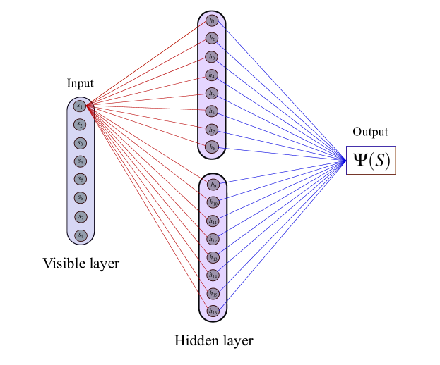
Figure 2: The schematic diagram for the ANN for a system size of $N=8$ and $M=16$, i.e., for $\gamma=2$. Each physical spin $s_{i}$ is connected to every hidden spin $h_{i}$ (only the connections of one physical spin for clarity). The final output is the probability amplitude $\Psi(S)$ of a given spin configuration $S$.

4 Artificial neural networks: RBM machine

In this section, we briefly describe the ANN method based on the RBM architecture, schematically shown in figure 2 [27, 28, 29, 31, 32]. In the RBM representation, the physical spins (neurons) $s_{i}\in(1,-1)$ in the primary layer are complemented by auxiliary layer of Ising spins (neurons) $h_{j}\in(1,-1)$. Each node in the primary layer is connected to each node in the auxiliary layer. There are no connections between nodes within a layer. The connection between $s_{i}$ and $h_{j}$ has a weight $w_{ij}$ which is $(ij)^{th}$ element of the weight matrix W. RBM has bias weights $b_{j}$ for the hidden units with $i=1,...,N$ and $j=1,...,M$ and we take $M=\gamma N$. In figure 2, we have shown a schematic representation of RBM for $N=8$ and $\gamma=2$. Now, the neural many-body quantum state (unnormalized) is defined as $\ket{\Psi}=\sum_{S}\Psi(S)\ket{S}$ with

$$\log(\Psi(S))=\sum_{j=1}^{M}\log\left[\cosh(b_{j}+\sum_{i=1}^{N}W_{ij}s_{i})\right]$$ (24)

and a spin configuration is given by $S=(s_{1},...,s_{N})$. $\Psi(S)$ determines the probability amplitude to find the particular spin configuration $S$. The dynamics is obtained using a time-dependent variational principle, which transforms the time-dependent Schrödinger equation into a set of non-linear symplectic differential equations for the variational parameters ${\bf x}=\{b_{j},W_{ij}\}$,

$$\dot{\bf x}(t)=-i\bf A^{-1}\bf F,$$ (25)

where $\bf x$ is composed of the variational parameters, ${\bf A}$ is a covariance matrix, and $\bf F$ is the generalized force. The elements of the matrix $\bf A$ and the vector $\bf F$ are

$${\bf A}_{kk^{\prime}}=\langle O^{*}_{k}O_{k^{\prime}}\rangle-\langle O^{*}_{k}\rangle\langle O_{k^{\prime}}\rangle$$ (26)

$${\bf F}_{k}=\langle O^{*}_{k}E_{\mathrm{loc}}\rangle-\langle O^{*}_{k}\rangle\langle E_{\mathrm{loc}}\rangle,$$ (27)

where $\langle...\rangle$ is taken over $\Psi(S)$, and $O^{*}_{k^{\prime}}(S)$ and $O_{k}(S)$ are variational derivatives given by

$$O_{k}(S)=\frac{1}{\Psi(S)}\frac{\partial\Psi(S)}{\partial x_{k}}$$ (28)

with $E_{\mathrm{loc}}$ being called the local energy, defined as

$$E^{S}_{\mathrm{loc}}({\bf x})=\frac{\langle S|\hat{H}|\Psi\rangle}{\langle S|\Psi\rangle}.$$ (29)

The equation (25) is then solved using the adaptive Heun scheme [69].

5 Excitation Dynamics

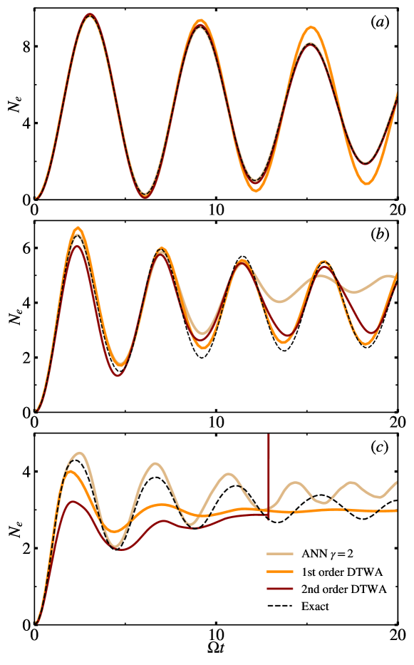
Figure 3: The dynamics of the total number of excitations ($N_{e}$) in an atomic chain of $N=10$ for different $\tilde{C}_{6}$. We compare the exact results (dashed line) with first and second-order DTWA and ANN (solid lines). (a) is for $\tilde{C}_{6}=0.2\Omega$, (b) for $\tilde{C}_{6}=\Omega$ and (c) is for $\tilde{C}_{6}=3\Omega$. For $\tilde{C}_{6}=0.2\Omega$, both ANN and second-order DTWA are in excellent agreement with exact results, but for large $\tilde{C}_{6}$, they deviate. ANN is found to be more reliable at large $\tilde{C}_{6}$. For ANN, we use $\gamma=2$. In (c), second-order DTWA experiences numerical instability at $\Omega t\approx 13$.

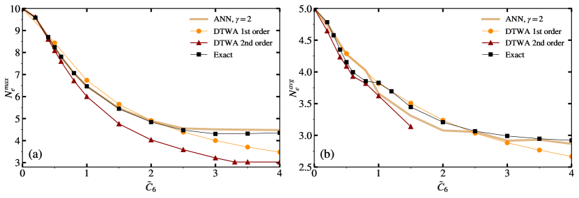
Figure 4: (a) The maximum ($N_{e}^{max}$) and (b) average ($N_{e}^{avg}$) number of excitations as a function of $\tilde{C}_{6}$ in a 10 atom chain. We compare the exact results with that of DTWA and ANN. For $N_{e}^{avg}$, we take an average over a period of $\Omega T=100$ for exact results, whereas for DTWA first order and ANN, we took $\Omega T=20$ and DTWA second order, we took $\Omega T=10$. The numerical instability in the secon-order DTWA limits the averaging period to smaller values.

In the following, we compare the Rydberg excitation dynamics obtained from DTWA and ANN to the exact results for $N=10$. The initial state is where all atoms are in their ground state. Figure 3 shows the dynamics of the total number of excitations $N_{e}(t)$ for different values of $\tilde{C}_{6}=C_{6}/d^{6}$. Initially, $N_{e}=0$, and as time evolves, $N_{e}$ increases and eventually oscillates in time. The oscillation amplitude is larger in the first cycle and damps over the subsequent cycles. For small $\tilde{C}_{6}$ [see figure 3(a)], both ANN and second-order DTWA show an excellent agreement with exact results. As seen, the first-order DTWA deviates from the exact dynamics at longer times, even for small interactions, indicating the importance of two-body correlations. As $\tilde{C}_{6}$ increases, the agreement with exact dynamics becomes lesser and lesser for both ANN and DTWA. The larger the $\tilde{C}_{6}$, the earlier the deviation from exact results occurs. At larger $\tilde{C}_{6}$ [figure 3(c)], second-order DTWA shows more deviation than first-order. It also suffers from numerical instability, and we anticipate that the higher-order BBGKY terms are vital. The latter are tedious to obtain, and numerical stability is generally not guaranteed. We also note that for larger $\tilde{C}_{6}$, oscillation amplitude shows a faster decay in DTWA results. Despite both ANN and DTWA failing at large interactions, the former is more reliable if short-time dynamics is desired.

In figure 4, we show the dependence of maximum ($N_{e}^{max}$), which is the amplitude of the first oscillation and average ($N_{e}^{avg}$) of $N_{e}$ on the interaction strength $\tilde{C}_{6}$. Both $N_{e}^{max}$ and $N_{e}^{avg}$ decrease with an increase in $\tilde{C}_{6}$ due to the blockade effect. For $\tilde{C}_{6}\ll\Omega$, we have $N_{e}^{max}\sim N$ and $N_{e}^{avg}\sim N/2$ and in a fully blockaded chain (limit $\tilde{C}_{6}\to\infty$) $N_{e}^{max}\sim 1$ and $N_{e}^{avg}\sim 1/2$. For $\tilde{C}_{6}>2\Omega$, in the exact results, $N_{e}^{max}\sim 5$ and $N_{e}^{avg}\sim 3$ saturate due to the nearest neighbor blockade, but the next nearest neighbor blockade requires an interaction strength of $\tilde{C}_{6}\sim 64\Omega$. Therefore, as a function of $\tilde{C}_{6}$, different plateaus for $N_{e}^{max}$ and $N_{e}^{avg}$ would emerge, indicating the blockades of atoms at larger separations. As far as $N_{e}^{max}$ and $N_{e}^{avg}$ are concerned, ANN is in excellent agreement with exact results even for large $\tilde{C}_{6}$.

For sufficiently small values of $\tilde{C}_{6}$ and at longer times, there exists collapse and revival of $N_{e}(t)$ about its average value [70], as shown in figure 5. A similar feature also arises in the population dynamics of a two-level atom coupled to a single-mode quantized light field in an optical cavity, described by the Jaynes-Cummings model (JCM). The collapse and revival in JCM are associated with the statistical and discrete nature of the photon field [71, 72]. In contrast, in the Rydberg chain, the collapse and revival in $N_{e}(t)$ can be attributed to the discrete nature (periodic lattice) of the physical setup. Both DTWA and ANN capture the collapse, but the revival is absent [see figure 5].

Figure 5: The long-time dynamics of $N_{e}(t)$ for $N=10$ and $\tilde{C}_{6}=0.2\Omega$. We compare the exact results with that of first-order DTWA and ANN. Although the collapse is captured by both methods, the revival is absent.

6 Correlation dynamics

6.1 Bipartite Rényi entropy

The quantum correlations in a many-body system are of significant importance, and here, we characterize them using the second-order Rényi entropy. The second-order Rényi entropy is defined as,

$$S^{(2)}_{A}(t)=-\frac{1}{N_{A}}\log({\rm Tr}[(\hat{\rho}_{A}(t)^{2})]),$$ (30)

where $N_{A}$ is the number of atoms in the subsystem $A$ and the reduced density matrix for the subsystem A is

$$\hat{\rho}_{A}(t)=\sum_{\alpha}\frac{1}{N_{s}}\hat{\mathcal{A}}^{\vec{\alpha}_{A}}_{1...N_{A}}(t),$$ (31)

where $\vec{\alpha}_{A}=\{\alpha_{1},\alpha_{2},...,\alpha_{N_{A}}\}$. In first-order DTWA, $\hat{\mathcal{A}}^{\alpha_{1}...\alpha_{N_{A}}}_{1...N_{A}}=\prod_{i\in A}\hat{\mathcal{A}}_{i}$ and the Rényi entropy takes the simple form [24],

$$S^{(2)}_{A}(t)=-\frac{1}{N_{A}}\log\left[\sum_{\alpha,\alpha^{\prime}}\frac{1}{N_{s}^{2}}\prod_{i\in A}\frac{1}{2}\left(\mathcal{I}+\sum_{\mu}a_{i}^{\mu}(t)a_{i}^{\prime\mu}(t)\right)\right],$$ (32)

where $a_{i}(0)={\bf r}_{\alpha_{i}}$ and $a^{\prime}_{i}(0)={\bf r}_{\alpha^{\prime}_{i}}$ are the initial conditions, which are evolved independently. In the second-order DTWA, additional correlation-dependent terms appear in equation (32). The computation of $S^{(2)}_{A}(t)$ in equation (32) involves a phase-space average weighted with two initial Wigner functions. In the case of ANN, the reduced density matrix can be directly obtained using the QuTiP, and then, we compute $S^{(2)}_{A}(t)$ using equation (30). We also calculate the mean two-site entropy,

$$\bar{S}^{(2)}(t)=\frac{1}{N-1}\sum_{\langle ij\rangle}S^{(2)}_{ij}(t)$$ (33)

Here, $S^{(2)}_{ij}$ is the 2nd order Rényi entanglement entropy for the subsystem containing two neighboring sites. Previously, it has been employed to study many-body localization and thermalization in a 1D Heisenberg model [73].

The dynamics of bipartite $S^{(2)}_{A}(t)$ for $N=10$ or $N_{A}=5$ is shown in figure 6. At $t=0$, we have $S^{(2)}_{A}(t)=0$ as we start in a product state where each atom is in $|g\rangle$. As time progresses, correlations build in the system, and $S^{(2)}_{A}(t)$ grows. Larger the $\tilde{C}_{6}$, faster the initial growth of the correlations. Even though first-order DTWA captured the population dynamics accurately for small $\tilde{C}_{6}$ [see figure 3(a)], it overestimates the Rényi entropy [see figure 6(a)]. In contrast, ANN captures the correlation dynamics accurately, and second-order DTWA shows agreement at shorter times. For large $\tilde{C}_{6}$, all methods fail to estimate the correlation dynamics accurately. We also noticed that $\hat{\mathcal{A}}_{i}$ in equation 11 is obtained by taking partial traces of $\hat{\mathcal{A}}^{\vec{\alpha}}_{1...N}(t)$ and hence, the purity of the density matrix determined by $\hat{\mathcal{A}}_{i}$ becomes less than unity, even though the system has no dissipative mechanism. Interestingly, the dynamics of mean two-site entropy [see figure 7] obtained from all methods shows better agreement with each other.

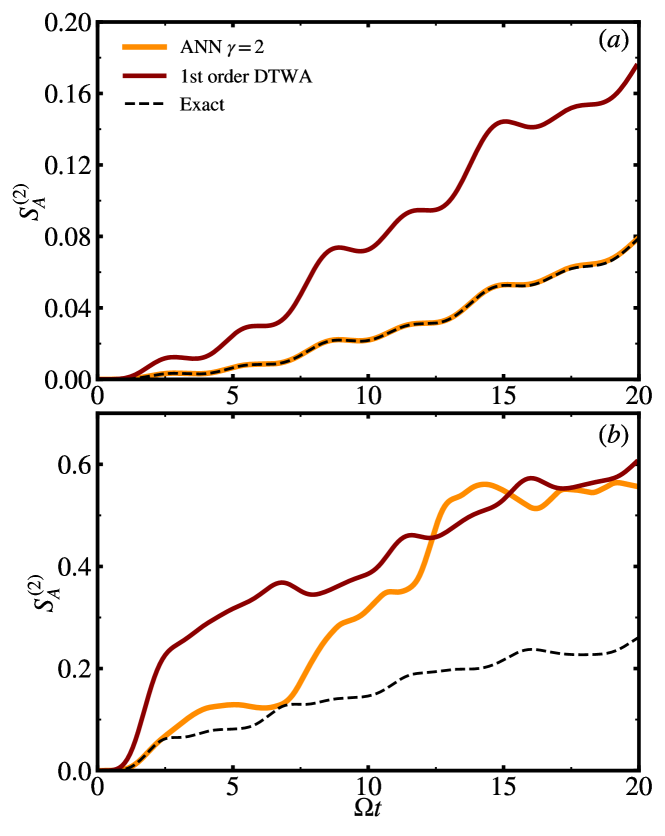
Figure 6: The dynamics of bipartite Rényi entanglement entropy for different (a) $\tilde{C}_{6}=0.2$ and (b) $\tilde{C}_{6}=1$. We compare the exact results with that of DTWA and ANN.

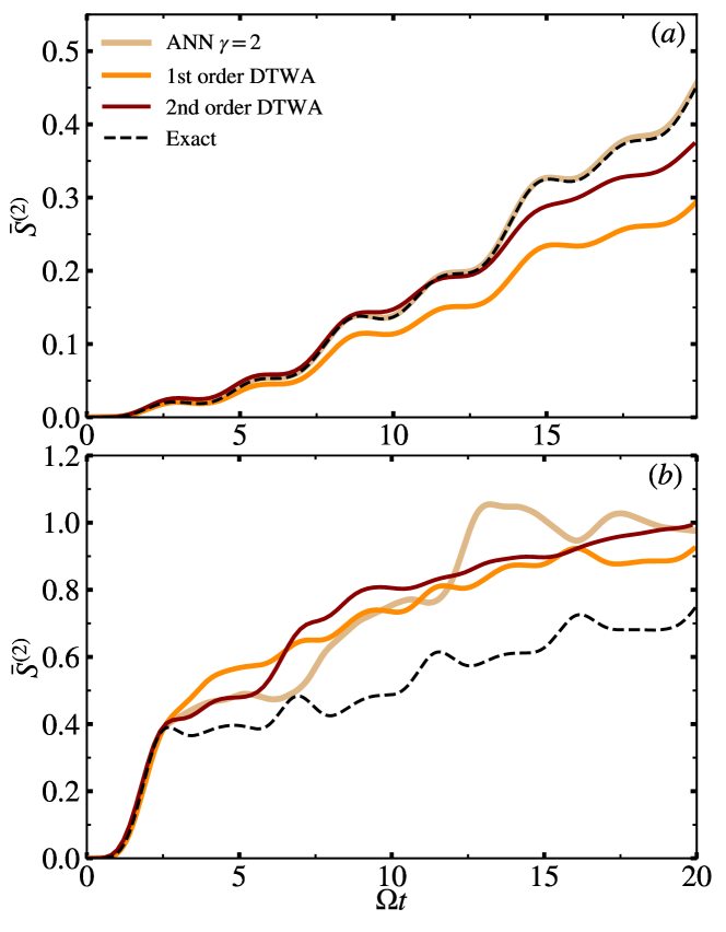
Figure 7: The dynamics of the mean two-site entropy for (a) $\tilde{C}_{6}=0.2$ and (b) $\tilde{C}_{6}=1$. We compare the exact results with that of DTWA and ANN.

7 Conclusions and Outlook

As the demand for numerical methods to capture the dynamics of quantum many-body systems is high, we benchmark DTWA and ANN based on RBM architecture using the exact results for the excitation and second-order Rényi entropy dynamics in a chain of ten two-level Rydberg atoms. In DTWA, we go beyond the mean-field approximation and include the two-body correlations via BBGKY hierarchy, which is generally a tedius task. DTWA and ANN methods are suitable for capturing the population dynamics when the Rydberg-Rydberg interactions are relatively small. Although the population dynamics showed deviations at large interaction strengths, the average number of excitations calculated via ANN shows good agreement with the exact results. Only ANN accurately reproduces the dynamics of quantum correlations for sufficiently long periods, whereas the second-order DTWA found to be good at small interaction strengths and shorter periods. In conclusion, both methods are not suitable to study the quantum Ising realizations using Rydberg atom lattices when the Rydberg-Rydberg interactions are significantly large.

We would like to see how these methods can be modified so that large interactions can be considered. Further, we would like to understand the instabilities in DTWA-BBGKY formalism. The same analysis can be extended to multi-dimensional setups, where the first-order DTWA, being a mean field, would work better and consider time-dependent Hamiltonians [42, 62, 64, 65, 66]. In particular, to analyze the formation of many-body states under quantum quenching, for instance, the dynamical crystallization [74]. Also, to incorporate the spontaneous emission from the Rydberg state and study the dissipative dynamics.

8 Acknowledgments

We acknowledge UKIERI-UGC Thematic Partnership No. IND/CONT/G/16-17/73 UKIERI-UGC project. W.L further thanks the support from the EPSRC through Grant No. EP/R04340X/1 via the QuantERA project ”ERyQSenS” and the Royal Society through the International Exchanges Cost Share award No. IEC$\backslash$NSFC$\backslash$181078.. R.N. further acknowledges DST-SERB for Swarnajayanti fellowship File No. SB/SJF/2020-21/19, and the MATRICS grant (MTR/2022/000454) from SERB, Government of India, and National Supercomputing Mission (NSM) for providing computing resources of ’PARAM Brahma’ at IISER Pune, which is implemented by C-DAC and supported by the Ministry of Electronics and Information Technology (MeitY) and Department of Science and Technology (DST), Government of India. V.N. acknowledges the funding from DST India through an INSPIRE scholarship. We also acknowledge funding from National Mission on Interdisciplinary Cyber-Physical Systems (NM-ICPS) of the Department of Science and Technology, Govt. Of India through the I-HUB Quantum Technology Foundation, Pune INDIA. Finally, we acknowledge QuSpin [75, 76], QuTiP [77, 78], and jVMC packages [79, 80].

References

- [1] Czischek, S 2020 Springer Theses, Springer Nature Switzerland
- [2] Orús R 2014 Ann. Phys. 349 117
- [3] White S R 1992 Phys. Rev. Lett. 69 2863
- [4] Vidal G 2004 Phys. Rev. Lett. 93 040502
- [5] Schollwöck U 2011 Ann. Phys. 326 96
- [6] Bridgeman J C, Chubb C T 2017 J. Phys. A: Math. Theor. 50 223001
- [7] White S R, Feiguin A E 2004 Phys. Rev. Lett. 93 076401
- [8] Polkovnikov A 2010 Ann. Phys. 325 1790
- [9] Blakie P B, Bradley A S, Davis M J, Ballagh R J, Gardiner C W 2008 Adv. Phys. 57 363
- [10] Schachenmayer J, Pikovski A, Rey A M 2015 New J. Phys. 17 065009
- [11] Schachenmayer J, Pikovski A, Rey A M 2015 Phys. Rev. X 5 011022
- [12] Pucci L, Roy A, Kastner M 2016 Phys Rev B 93 174302
- [13] Zhu B, Rey A M, Schachenmayer J 2019 New J. Phys. 21 082001
- [14] Wurtz J, Polkovnikov A, Sels D 2018 Ann. Phys. 395 341
- [15] Huber J, Rey A M and Rabl P arXiv:2105.00004
- [16] Khasseh R, Russomanno A, Schmitt M, Heyl M, and Fazio R 2020 Phys. Rev. B 102 014303
- [17] Orioli A P, Signoles A, Wildhagen H, Günter G, Berges J, Whitlock S and Weidemüller M 2018 Phys. Rev. Lett. 120 063601
- [18] Signoles A, Franz T, Alves R F, Gärttner M, Whitlock S, Zürn G and Weidemüller M 2021Phys. Rev. X 11 011011
- [19] Geier S et al arXiv:2105.01597
- [20] Hao L et al 2021 New J. Phys. 23 083017
- [21] Lepoutre S, Schachenmayer J, Gabardos L, Zhu B, Naylor B, Maréchal E, Gorceix O, Rey A M, Vernac L and Laburthe-Tolra B 2019 Nat. Commun. 10 1714
- [22] Fersterer P et al 2019 Phys. Rev. A 100 033609
- [23] Patscheider A 2020 Phys. Rev. Research 2 023050
- [24] Kunimi M, Nagao K, Goto S and Danshita I 2021 Phys. Rev. Research 3 013060
- [25] Mehta P, Bukov M, Wang C-H, Day A G R, Richardson C, Fisher C K, Schwab D J 2019 Phys. Rep. 810 1-124
- [26] Carleo G, Cirac I, Cranmer K, Daudet L, Schuld M, Tishby N, Vogt-Maranto L, Zdeborová L 2019 Rev. Mod. Phys.91 045002
- [27] Carleo G, and Troyer M 2017 Science 355 602
- [28] Fabiani G, and Mentink J H 2019 SciPost Phys. 7 004
- [29] Czischek S, Gärttner M, and Gasenzer T 2018 Phys. Rev. B 98 024311
- [30] Wu Y, Duan L M, and Deng D L 2020 Phys. Rev. B 101 214308
- [31] Deng D L, Li X, and Sarma S D 2017 Phys. Rev. X 7 021021
- [32] Deng D L, Li X, and Sarma S D 2017 Phys. Rev. B 96 195145
- [33] Browaeys A, and Lahaye T 2020 Nat. Phys. 16 132
- [34] Bernien H, Schwartz S, Keesling A, Levine H, Omran A, Pichler H, Choi S, Zibrov A S, Endres M, Greiner M, Vuletić V, and Lukin M D 2017 Nature 551, 579
- [35] Schlosser M, Ohl de Mello D, Schäffner D, Preuschoff T, Kohfahl L and Birkl G 2020 J. Phys. B: At. Mol. Opt. Phys. 53 144001
- [36] Kim H, Park Y, Kim K, Sim H-S and Ahn J 2018 Phys. Rev. Lett. 120 180502
- [37] Guardado-Sanchez E, Brown P T, Mitra D, Devakul T, Huse D A, Schauß P, and Bakr W S 2018 Phys. Rev. X 8 021069
- [38] Labuhn H, Barredo D, Ravets S, De Léséleuc S, Macrì T, Lahaye T and Browaeys A 2016 Nature 534 667
- [39] Graham T M, Kwon M, Grinkemeyer B, Marra Z, Jiang X, Lichtman M T, Sun Y, Ebert M, and Saffman M 2019 Phys. Rev. Lett. 123 230501
- [40] Scholl P, Schuler M, Williams H J, Eberharter A A, Barredo D, Schymik K-N, Lienhard V, Henry L-P, Lang T C, Lahaye T, Läuchli A M, and Browaeys A, Nature 595 233
- [41] Ebadi S, Wang T T, Levine H, Keesling A, Semeghini G, Omran A, Bluvstein D, Samajdar R, Pichler H, Ho W W, Choi S, Sachdev S, Greiner M, Vuletic V, and Lukin M D, Nature 595 227
- [42] Bluvstein D, Omran A, Levine H, Keesling A, Semeghini G, Ebadi S, Wang T T, Michailidis A A, Maskara N, Ho W W, Choi S, Serbyn M, Greiner M, Vuletić V, and Lukin M D, 2021 Science 371 1355
- [43] Saffman M, Walker T G, and Mølmer K 2010 Rev. Mod. Phys. 82 2313
- [44] Béguin L, Vernier A, Chicireanu R, Lahaye T and Browaeys A 2013 Phys. Rev. Lett. 110 263201
- [45] Lukin M D, Fleischhauer M, Cote R, Duan L M, Jaksch D, Cirac J I. and Zoller P 2001 Phys. Rev. Lett. 87 037901
- [46] Gaëtan A, Miroshnychenko Y, Wilk T, Chotia A, Viteau M, Comparat D, Pillet P, Browaeys A and Grangier P 2009 Nat. Phys. 5 115
- [47] Urban E, Johnson T A, Henage T, Isenhower L, Yavuz D D, Walker T G and Saffman M 2009 Nature Physics 5 110
- [48] Weimer H, Müller M, Lesanovsky I., Zoller P and Büchler H P 2010 Nat. Phys. 6 382
- [49] Mukherjee R, Millen J, Nath R, Jones M P A, and Pohl T 2011 J. Phys. B: At. Mol. Opt. Phys. 44 184010
- [50] Schauß P, Cheneau M, Endres M, Fukuhara T, Hild S, Omran A, Pohl T, Gross C, Kuhr S and Bloch I 2012 Nature 491 87
- [51] Barredo D, Labuhn H, Ravets S, Lahaye T, Browaeys A and Adams C S 2015 Phys. Rev. Lett. 114 113002
- [52] Zeiher J, Van Bijnen R, Schauß P, Hild S, Choi J Y, Pohl T, Bloch I and Gross C 2016 Nat. Phys. 12 1095
- [53] Zeiher J, Choi J Y, Rubio-Abadal A, Pohl T, van Bijnen R, Bloch I and Gross, C 2017 Phys. Rev. X 7 041063
- [54] Marcuzzi M, Minář J C V, Barredo D, de Léséleuc S, Labuhn H, Lahaye T, Browaeys A, Levi E and Lesanovsky I 2017 Phys. Rev. Lett. 118 063606
- [55] Gross C and Bloch I 2017 Science 357 995
- [56] Jaksch D, Cirac J I, Zoller P, Rolston S L, Côté R and Lukin M D 2000 Phys. Rev. Lett. 85 2208
- [57] Wilk T, Gaëtan A, Evellin C, Wolters J, Miroshnychenko Y, Grangier P and Browaeys A 2010 Phys. Rev. Lett. 104 010502
- [58] Isenhower L, Urban E, Zhang X L, Gill A T, Henage T, Johnson T A, Walker T G and Saffman M 2010 Phys. Rev. Lett. 104 010503
- [59] Saffman M 2016 J. Phys. B: At. Mol. Opt. Phys. 49 202001
- [60] Su S.-L., Guo F.-Q., Wu J.-L. , Jin Z, Shao X Q, and Zhang S 2020 Europhys. Lett. 131, 53001
- [61] Xiaoling Wu et al 2021 Chinese Phys. B 30 020305
- [62] Basak S, Chougale Y, and Nath R 2018 Phys. Rev. Lett. 120 123204
- [63] Glaetzle A W, Nath R, Zhao B, Pupillo G, and Zoller P 2012 Phys. Rev. A 86 043403
- [64] Niranjan A, Li W, and Nath R 2021 Phys. Rev. A 101 063415
- [65] Mallavarapu S K, Niranjan A, Li W, Wüster S, and Nath R 2021 Phys. Rev. A 103 023335
- [66] Varghese D, Wüster S, Li W, and Nath R 2023 Phys. Rev. A 107 043311
- [67] Wootters W K 1987 Ann. Phys. 176 1
- [68] Wootters W K 2003 arXiv:quant-ph/0306135
- [69] Schmitt M and Heyl M 2020 Phys. Rev. Lett. 125 100503
- [70] Wu G, Kurz M, Liebchen B, and Schmelcher P 2015 Phys. Lett. A 379 143
- [71] Eberly J H, Narozhny N B, and Sanchez-Mondragon J J 1980 Phys. Rev. Lett. 44 1323
- [72] Rempe G, Herbert W, and Klein N 1987 Phys. Rev. Lett. 58 353
- [73] Acevedo O L, Safavi-Naini A, Schachenmayer J, Wall M L, Nandkishore R, and Rey A M 2017 Phys. Rev. A 96 033604
- [74] Pohl T, Demler E, Lukin M D 2010 Phys. Rev. Lett. 104 043002
- [75] Weinberg P and Buko M 2017 SciPost Phys. 2 003
- [76] Weinberg P and Buko M 2019 SciPost Phys. 7 020
- [77] Johansson J R, Nation P D, and Nori F 2012 Computer Physics Communications 183 1760
- [78] Johansson J R, Nation P D, and Nori F 2013 Computer Physics Communications 184 1234
- [79] Schmitt M and Reh M 2022 SciPost Phys. Codebases 2-r0.1
- [80] Schmitt M and Reh M 2022 SciPost Phys. Codebases 2