Monte Carlo simulations of biaxial molecules near a hard wall
Abstract
A system of optimal biaxial molecules placed at the sites of a cubic lattice is studied in an extended Lebwohl-Lasher model. Molecules interact only with their nearest neighbors through the pair potential that depends on the molecule orientations. It is known that in the homogeneous system there is a direct second-order transition from the isotropic to the biaxial nematic phase, but properties of confined systems are less known. In the present paper the lattice has periodic boundary conditions in the X and Y directions and it has two walls with planar anchoring, perpendicular to the Z direction. We have investigated the model using Monte Carlo simulations on lattices, , from 3 to 19, with and without assuming mirror symmetry. This study is complementary to the statistical description of hard spheroplatelets near a hard wall by Kapanowski and Abram [Phys. Rev. E 89, 062503 (2014)]. The temperature dependence of the order-parameter profiles between walls is calculated for many wall separations. For large wall separations there are the surface layers with biaxial ordering at both walls (4-5 lattice constants wide) and beyond the surface layers the order parameters have values as in the homogeneous system. For small wall separations the isotropic-biaxial transition is shifted and the surface layers are thinner. Above the isotropic-biaxial transition the preferable orientations in both surface layers can be different. It is interesting that planar anchoring for biaxial molecules leads to the uniaxial interactions at the wall. As a result we get the planar Lebwohl-Lasher model with additional (biaxial) interactions with the neighbors from the second layer, where the Kosterlitz-Thouless transition is present.
pacs:
61.30.Cz, 77.84.NhI Introduction
Biaxial nematic phases are characterized by an orientational order along three perpendicular directions and by the existence of three distinct optical axes. Such phases were first predicted by Freiser in 1970 Freiser (1970). Later, biaxial phases have been studied by mean field theory Straley (1974), Luckhurst et al. (1975), Mulder and Ruijgrok (1982), counting methods (a generalization of a Flory’s lattice model) Shih and Alben (1972), Li and Freed (1994), bifurcation analysis Mulder (1989), and other methods, including computer simulations Allen (1990), Camp and Allen (1997), Skutnik et al. (2020). Motivation for these studies ranges from purely academic interest to the potential usage of biaxial nematics in faster displays.
Straley obtained a phase diagram for a system of biaxial molecules using mean field theory Straley (1974). He showed that four order parameters are necessary to describe ordered phases with biaxial molecules. The same was confirmed by Mulder, who derived also the analitical formula for the excluded volume for a pair of spheroplatelets which are biaxial objects Mulder (1986).
First theories predict that the system of biaxial molecules can exhibit four phases, depending on the molecular biaxiality: the positive uniaxial phase (, with prolate molecules), the negative uniaxial phase (, with oblate molecules), the biaxial phase (), and the isotropic phase (). The nematic-isotropic phase transition is weakly first order and it becomes continous at the point of maximum molecular biaxiality. At this point there is a direct transition from the biaxial to the isotropic phase.
Later theories showed that phase transitions to the biaxial phase can be either first or second order with the possibility of several critical points and reentrant biaxial nematic phases Allender and Longa (2008). In some phase diagrams three different biaxial phases were identified, where two additional biaxial phases were connected with mixtures of rodlike and platelike molecules Mukherjee and Sen (2009).
I.1 Lattice models
The Lebwohl-Lasher (LL) model is a lattice version of the Maier-Saupe model of anisotropic liquids with uniaxial molecules Lebwohl and Lasher (1972), Fabbri and Zannoni (1986). A weak first-order nematic-isotropic phase transition was found in the three-dimensional model at for lattice sizes up to Zhang et al. (1992). Pretransitional fluctuations of the LL model were studied by Greeff and Lee Greeff and Lee (1994). A large lattice of was studied on a parallel supercomputer and the temperature dependence of the energy, the order parameter and the heat capacity was obtained with greater accuracy Boschi et al. (1997). The effect of an external field on a nematic system was also investigated and the change in the character of the transition from first to second order with disappearance of the transition at a critical point was observed.
A biaxial version of the LL model was studied by Biscarini et al. Biscarini et al. (1995). They determined the phase diagram of the lattice model for varying biaxiality. The full set of four second rank order parameters was calculated for the first time and differences from mean field theory were discussed.
I.2 Molecules at the interface
The properties of the nematic-isotropic phase transition in thin nematic films were studied for the first time by Sheng Sheng (1976). He used the Landau-de Gennes theory to show the existence of a critical thickness of the film below which the transition from the nematic phase to the isotropic phase becomes continuous. Later this framework was used to describe a boundary-layer phase transition which occurs at temperatures higher than the bulk-transition temperature Sheng (1982).
A thin cell with hard spherocylinders was studied by Mao et al. Mao et al. (1997a). Spherocylinders are composed of cylinders of the length , the diameter , and hemispherical end caps. Grand canonical Monte Carlo simulations were used to investigate the effect of finite aspect ratio in density profiles and in order parameters (). The wall effect penetrated the bulk to a distance of order . No biaxial order was present in the simulated system if the phase was isotropic in the bulk. In the next paper by Mao et al. the depletion force was studied in the confined geometry of two parallel plates Mao et al. (1997b).
In 2000 van Roij et al. investigated the phase behavior of hard-rod fluid near a single wall and confined in slit pore van Roij et al. (2000a), van Roij et al. (2000b). They showed a wall-induced surface transition from uniaxial to biaxial symmetry and complete orientational wetting of the wall-isotropic fluid interface by a nematic film. Theoretical analysis was done by employing Zwanzig’s rod-model where the molecules are restricted to orientations which are parallel to one of the Cartesian coordinate axes. The results were confirmed by Monte Carlo simulations of a fluid of hard spherocylinders with Dijkstra et al. (2001).
Liquid crystals confined between parallel walls were studied by Allen Allen (2000). Computer simulations were compared with the theoretical predictions of Onsager’s density-functional theory. Several different anchoring conditions at the wall-nematic interface were investigated. In all cases, the principal effect of increasing the average density is to increase the surface film thicknes.
A density-functional treatment of a hard Gaussian overlap fluid confined between two parallel hard walls was presented by Chrzanowska et al. Chrzanowska et al. (2001). For uniaxial particles of elongation 5, the density and the order parameter profiles were obtained in the Onsager approximation. The surface layers of thickness about half of a particle length were present with the uniaxial and biaxial order, in the case of the isotropic and uniaxial phase in the bulk, respectively.
The effect of the incomplete interaction on the nematic-isotropic transition at the nematic-wall interface was studied by Batalioto et al. Batalioto et al. (2004). They used an extended Maier-Saupe approach with additional interactions with the wall. In this framework they showed the existence of a boundary layer in which the order parameter can be greater or smaller than the one in the bulk, according to the strength of the surface potential with respect to the nematic one.
The equilibrium phase behavior of a confined rigid-rod system was studied by Green et al. Green et al. (2010). The distribution functions for stable and unstable equilibrium states were computed as a function of the system density and the system width. The surprising conclusion was that the introduction of walls perturbs the stability limits for any system width, which means that walls always impact the interior of systems.
Aliabadi et al. examined the ordering properties of rectangular hard rods at a single planar wall and between two parallel hard walls using the second virial density-functional theory in the Zwanzig approximation Aliabadi et al. (2015). The most interesting finding for the slit pore is the first-order transition from the surface ordered isotropic to the capillary nematic phase. This transition weakens with decreasing pore width and terminates in a critical point.
A system of hard spheroplatelets near a hard wall was studied in the low-density Onsager approximation by Kapanowski and Abram Kapanowski and Abram (2014). Spheroplatelets had optimal shape between rods and plates, and the direct transition from the isotropic to the biaxial nematic phase was present in the bulk. For the one-particle distribution function a simple approximation was used and as a result the order parameters were equal to their bulk values unless we were in the interfacial region thinner then the molecule length. Biaxiality close to the wall appeared only if the phase was biaxial in the bulk. For the case of the isotropic phase in the bulk, the phase near the wall was uniaxial (oblate).
Our aim in the present paper is to get more realistic order parameter profiles between two walls and check the width of the interfacial region for the system of biaxial molecules with the direct transition from the isotropic to the biaxial nematic phase. This paper is organized as follows. The lattice model of biaxial molecules is described in Sec. II. In Sec. III we present the results of Monte Carlo simulations of the homogeneous and confined systems. Section IV contains the summary.
II System
We have considered a system of optimal biaxial molecules placed at the sites of a cubic lattice . The orientation of a rigid molecule can be determined by several methods: by the three Euler angles , by the three orthonormal vectors , by the orthogonal rotation matrix, and by the unit quaternion Vesely (1982). We are using quaternions in simulations because they are compact, stable numerically, and we do not have to use slow trigonometric functions. Our calculations are based on the second rank pair potential Luckhurst et al. (1975), Biscarini et al. (1995),
| (1) |
where is the relative orientation of the molecule pair, is equal to a positive constant for nearest neighbors and zero otherwise. The biaxiality parameter accounts for the deviation from cylindrical molecular symmetry. For the Lebwohl-Lasher model is recovered. The value marks the boundary between a system of prolate () and oblate molecules (). In our study we focus on the most biaxial molecules so . Note that , where was used in Biscarini et al. (1995); the difference comes from different definitions of symmetry-adapted functions. The functions are defined in Ref. Kapanowski (1997) and they are related to Wigner functions . The most important functions are
| (2) |
| (3) |
| (4) |
| (5) |
where is the second Legendre polynomial. For the completely ordered system with all molecule orientations parallel to the walls we get , where is the number of molecules (lattice sites).
We have performed Monte Carlo (MC) simulations with three different boundary conditions. (i) Periodic boundary conditions in the three directions are for the homogeneous system. (ii) Periodic boundary conditions in the two directions and two walls at and with planar anchoring are for the confined systems, is the lattice constant. The distance between walls is . (iii) Periodic boundary conditions in the two directions , the wall at with planar anchoring, and mirror symmetry applied at ; this corresponds to , but less computer resources are needed for simulations. We will compare the results from different simulations when the conditions (ii) and (iii) describe the same physical system. Planar anchoring at the walls is motivated by the fact that elongated molecules can be closer to the wall only if they are parallel to the wall. On the other hand, the isotropic-nematic interface favors planar anchoring Allen (2000).
Let us move to the determination of the order parameters and their temperature dependence. In computer simulations of homogeneous systems three tensors are typically used Allen (1990), Camp and Allen (1997), Biscarini et al. (1995)
| (6) |
| (7) |
| (8) |
Through a diagonalization of these tensors one could determine the order parameters according to the procedure described in Biscarini et al. (1995). The nontrivial problem is finding a consistent way of assigning the three eigenvalues to the axes. In our confined systems all three tensors , , are calculated independently for all layers parallel to the walls. Then the axis is always perpendicular to the walls and the axis is parallel to the walls and corresponds to the maximum eigenvalue of the tensor . Finally, four order parameters are calculated
| (9) |
| (10) |
| (11) |
| (12) |
Note that the same order parameters must have the same values in all the ways they are computed. The values of the order parameters depend on the phase orientation. For the completely ordered system there are six main phase orientations which are sumarized in Table 1. The order parameter is a measure of the alignment of the molecule axis along the axis of the reference frame. The order parameter describes the relative distribution of the and the axes along the axis. Both and can be nonzero in the uniaxial nematic phase. The order parameter describes the relative distribution of the axis along the and the axes. The order parameter is related to the distributions of the and axes along the and the axes. Both and signal biaxiality of the phase.
| OP | (homogeneous) | (confined) | ||||
|---|---|---|---|---|---|---|
III Results
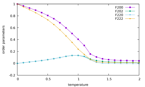
Prior to study the confined systems we have calculated the homogeneous bulk system and the temperature dependence of the order parameters, as shown in Fig. 1. We have performed MC simulations on and lattices with periodic boundary conditions in all three directions. The temperature step was typically and near the transition. We have used lattice cycles for warmup and cycles for production, where a cycle is attepted moves. Sometimes cycles were used as an additional check. We started from the ideal configuration at the lowest temperature, then the last configuration for a given temperature was used as the initial configuration for the next temperature. Figure 1 shows that the biaxial-isotropic transition is near , in agreement with Biscarini et al. (1995). The energy of the homogeneous system is always negative and it is an increasing function of temperature.
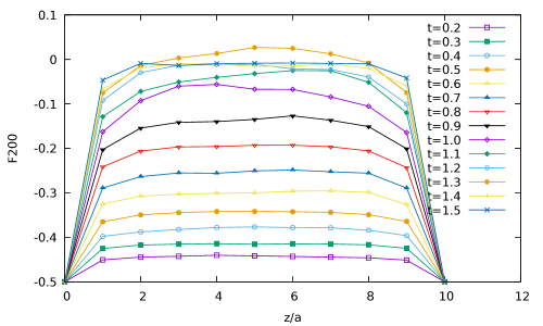
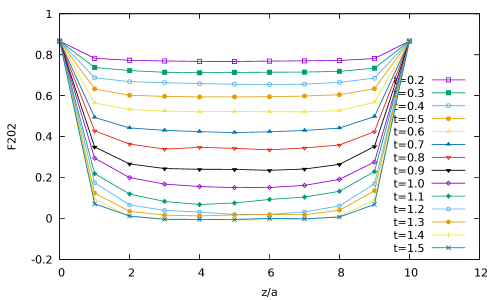
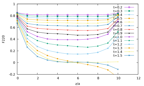
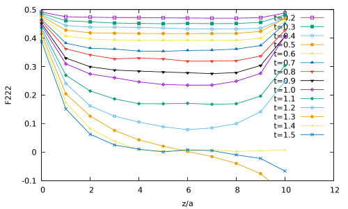
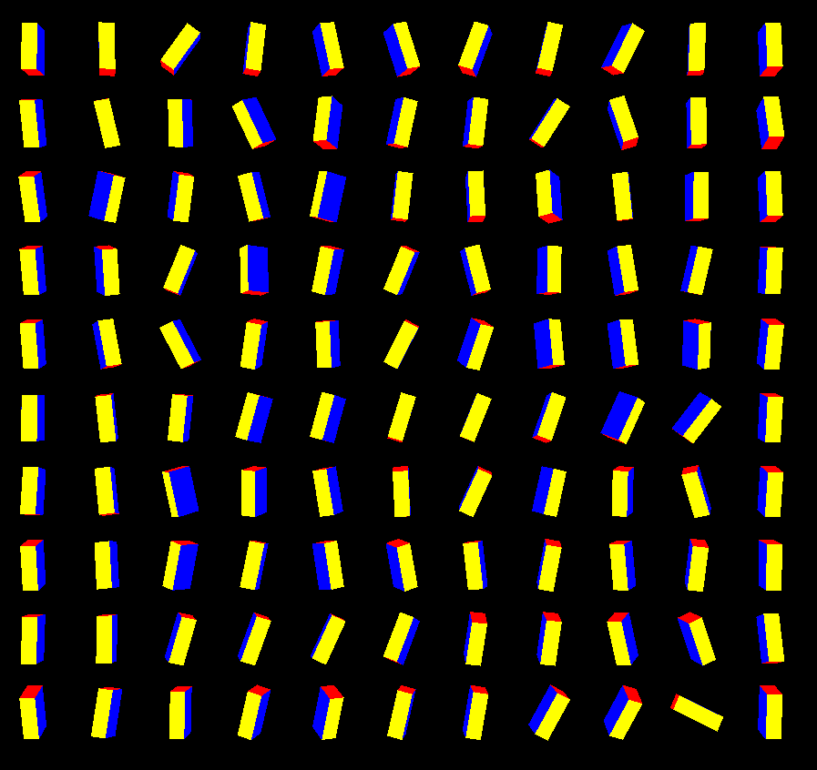
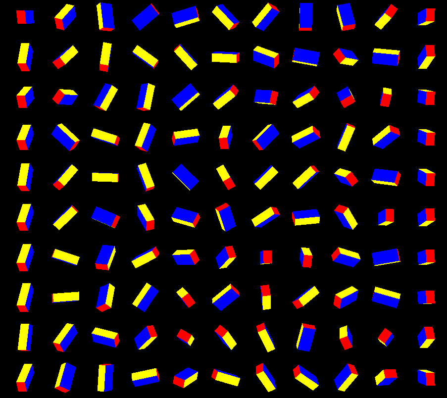
Let us move to the description of the confined systems. We have performed MC simulations on lattices, from 3 to 19, with periodic boundary conditions in the directions and two parallel walls with planar anchoring. Figures from 2 to 5 show the order parameters profiles for the lattice system . In the isotropic phase () the order parameters are almost zero except in the surface layers of the length approximately 4-5 lattice constants. Near the walls long molecule axes are nearly parallel to the walls and this yields , with the expected limit of at the walls. On decreasing temperature, a transition take place to the biaxial nematic phase, at which all order parameters become finite beyond the surface layers. Snapshots of simulation configurations in the biaxial nematic and in the isotropic phases are given in Fig. 6 and Fig. 7, respectively. In the biaxial nematic phase the preferable orientation of molecules on both walls is the same, although it is changing during computations. In the isotropic phase different preferable orientations on the walls are common and it is visible in the snapshots and the order parameter profiles. We note that this effect can not be obtained using the boudary conditions with mirror symmetry. What is more, we have got unphysical effects in the cell center, probably due to inconsistency in the formula for the total energy of the system.
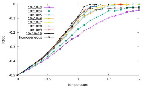
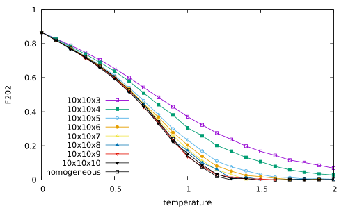
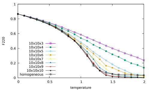
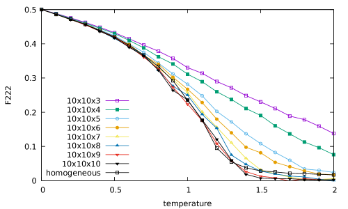
Figures from 8 to 11 show the temperature dependence of the order parameters in the cell center. The temperature of the isotropic-biaxial transition is shifted but for it is almost the same as in the homogeneous system. From this point the surface layers are separated and they have both biaxial nematic ordering ( is nonzero). We note a small discrepancy between the results for the homogeneous system and for the confined systems. This is due to numerical errors during diagonalization of the tensors . The results for the confined systems are more exact because at the wall one axis is fixed as perpendicular to the wall. For and the biaxial nematic phase is present is the cell for higher temperatures but the order parameters monotonically go to zero. We have not found any capilary nematization transition.
IV Conclusions
In this work we have studied the order-parameter profiles in the confined systems of optimal biaxial molecules using Monte Carlo simulations in an extended Lebwohl-Lasher model. In the homogeneous system there is a direct second-order isotropic-biaxial transition. We have studied the confined systems with two parallel walls with planar anchoring and with different wall separations.
For large wall separations there are the surface layers at both walls with the width of 4-5 lattice constants and beyond the surface layers the order parameters have values as in the homogeneous system. The ordering within the surface layers is always biaxial wheres in the paper Kapanowski and Abram (2014) biaxiality close to the wall was present only if the phase was biaxial in the bulk. The reason for this discrepancy is planar anchoring at the walls which creates the planar (uniaxial) Lebwohl-Lasher model with the Kosterlitz-Thouless transition Chiccoli et al. (1988), Mondal and Roy (2003). In our systems there are additional (biaxial) interactions with neighbors in the second layer. The partial ordering at the walls in our finite systems creates the biaxial ordering in the surface layers for all temperatures. We note that the surface transition was studied, for uniaxial molecules and different surface couplings, using the Landau-de Gennes approach L’vov et al. (1993), Kothekar et al. (1994). Additional effects due to external fields were studied in Ito et al. (2005) but again for uniaxial molecules.
For small wall separations the isotropic-biaxial transition is shifted to higher temperatures and the surface layers are thinner. The preferable orientation of the biaxial nematic phase is approximately the same near the walls and in the center of the cell but its direction can change during simulations. Above the isotropic-biaxial transition the preferable orientations in both surface layers can be different.
In summary, the presented results of MS simulations revealed effects which combine the properties of two-dimensional and three-dimensional systems. It is important to study systems with biaxial molecules using different techniqes in order to better understand the biaxial nematic phases and to find hints for experiments.
References
- Freiser (1970) M. J. Freiser, Phys. Rev. Lett. 24, 1041 (1970).
- Straley (1974) J. P. Straley, Phys. Rev. A 10, 1881 (1974).
- Luckhurst et al. (1975) G. Luckhurst, C. Zannoni, P. Nordio, and U. Segre, Molecular Physics 30, 1345 (1975), https://doi.org/10.1080/00268977500102881 .
- Mulder and Ruijgrok (1982) B. Mulder and T. Ruijgrok, Physica A: Statistical Mechanics and its Applications 113, 145 (1982).
- Shih and Alben (1972) C. Shih and R. Alben, The Journal of Chemical Physics 57, 3055 (1972), https://doi.org/10.1063/1.1678719 .
- Li and Freed (1994) W. Li and K. F. Freed, The Journal of Chemical Physics 101, 519 (1994), https://doi.org/10.1063/1.468162 .
- Mulder (1989) B. Mulder, Phys. Rev. A 39, 360 (1989).
- Allen (1990) M. P. Allen, Liquid Crystals 8, 499 (1990), https://doi.org/10.1080/02678299008047365 .
- Camp and Allen (1997) P. J. Camp and M. P. Allen, The Journal of Chemical Physics 106, 6681 (1997), https://doi.org/10.1063/1.473665 .
- Skutnik et al. (2020) R. A. Skutnik, I. S. Geier, and M. Schoen, Molecular Physics 118, e1726520 (2020), https://doi.org/10.1080/00268976.2020.1726520 .
- Mulder (1986) B. M. Mulder, Liquid Crystals 1, 539 (1986), https://doi.org/10.1080/02678298608086278 .
- Allender and Longa (2008) D. Allender and L. Longa, Phys. Rev. E 78, 011704 (2008).
- Mukherjee and Sen (2009) P. K. Mukherjee and K. Sen, The Journal of Chemical Physics 130, 141101 (2009), https://doi.org/10.1063/1.3117925 .
- Lebwohl and Lasher (1972) P. A. Lebwohl and G. Lasher, Phys. Rev. A 6, 426 (1972).
- Fabbri and Zannoni (1986) U. Fabbri and C. Zannoni, Molecular Physics 58, 763 (1986).
- Zhang et al. (1992) Z. Zhang, O. G. Mouritsen, and M. J. Zuckermann, Phys. Rev. Lett. 69, 2803 (1992).
- Greeff and Lee (1994) C. W. Greeff and M. A. Lee, Phys. Rev. E 49, 3225 (1994).
- Boschi et al. (1997) S. Boschi, M. P. Brunelli, C. Zannoni, C. Chiccoli, and P. Pasini, International Journal of Modern Physics C 08, 547 (1997), https://doi.org/10.1142/S0129183197000436 .
- Biscarini et al. (1995) F. Biscarini, C. Chiccoli, P. Pasini, F. Semeria, and C. Zannoni, Phys. Rev. Lett. 75, 1803 (1995).
- Sheng (1976) P. Sheng, Phys. Rev. Lett. 37, 1059 (1976).
- Sheng (1982) P. Sheng, Phys. Rev. A 26, 1610 (1982).
- Mao et al. (1997a) Y. Mao, P. Bladon, H. N. W. Lekkerkerker, and M. E. Cates, Molecular Physics 92, 151 (1997a), https://doi.org/10.1080/002689797170716 .
- Mao et al. (1997b) Y. Mao, M. E. Cates, and H. N. W. Lekkerkerker, The Journal of Chemical Physics 106, 3721 (1997b), https://doi.org/10.1063/1.473424 .
- van Roij et al. (2000a) R. van Roij, M. Dijkstra, and R. Evans, Europhysics Letters (EPL) 49, 350 (2000a).
- van Roij et al. (2000b) R. van Roij, M. Dijkstra, and R. Evans, The Journal of Chemical Physics 113, 7689 (2000b), https://doi.org/10.1063/1.1288903 .
- Dijkstra et al. (2001) M. Dijkstra, R. v. Roij, and R. Evans, Phys. Rev. E 63, 051703 (2001).
- Allen (2000) M. P. Allen, The Journal of Chemical Physics 112, 5447 (2000), https://doi.org/10.1063/1.481112 .
- Chrzanowska et al. (2001) A. Chrzanowska, P. I. C. Teixeira, H. Ehrentraut, and D. J. Cleaver, Journal of Physics: Condensed Matter 13, 4715 (2001).
- Batalioto et al. (2004) F. Batalioto, L. Evangelista, and G. Barbero, Physics Letters A 324, 198 (2004).
- Green et al. (2010) M. J. Green, R. A. Brown, and R. C. Armstrong, Journal of Computational and Theoretical Nanoscience 7, 693 (2010).
- Aliabadi et al. (2015) R. Aliabadi, M. Moradi, and S. Varga, Phys. Rev. E 92, 032503 (2015).
- Kapanowski and Abram (2014) A. Kapanowski and M. Abram, Phys. Rev. E 89, 062503 (2014).
- Vesely (1982) F. J. Vesely, Journal of Computational Physics 47, 291 (1982).
- Kapanowski (1997) A. Kapanowski, Phys. Rev. E 55, 7090 (1997).
- Chiccoli et al. (1988) C. Chiccoli, P. Pasini, and C. Zannoni, Physica A: Statistical Mechanics and its Applications 148, 298 (1988).
- Mondal and Roy (2003) E. Mondal and S. K. Roy, Physics Letters A 312, 397 (2003).
- L’vov et al. (1993) Y. L’vov, R. M. Hornreich, and D. W. Allender, Phys. Rev. E 48, 1115 (1993).
- Kothekar et al. (1994) N. Kothekar, D. W. Allender, and R. M. Hornreich, Phys. Rev. E 49, 2150 (1994).
- Ito et al. (2005) M. Ito, M. Torikai, and M. Yamashita, Molecular Crystals and Liquid Crystals 441, 69 (2005), https://doi.org/10.1080/154214091009554 .