Upper bound on the rate of convergence and truncation bound
for non-homogeneous birth and death processes on
Y. A. Satin111Vologda State University; e-mail yacovi@mail.ru,
R. V. Razumchik222Federal Research Center “Computer Science and Control” of the Russian Academy of Sciences; Moscow Center for Fundamental and Applied Mathematics; e-mail rrazumchik@ipiran.ru,
A. I. Zeifman333Vologda State University; Federal Research Center “Computer Science and Control” of the Russian Academy of Sciences; Moscow Center for Fundamental and Applied Mathematics; Vologda Research Center RAS; e-mail azeifman@mail.ru,
I. A. Kovalev444Vologda State University; e-mail kovalev.iv96@yandex.ru
Abstract
We consider the well-known problem of the computation of the (limiting) time-dependent performance
characteristics of one-dimensional continuous-time birth and death processes
on with time varying and possible state-dependent intensities.
First in the literature upper bounds on the rate of convergence
along with one new concentration inequality are provided.
Upper bounds for the error of truncation are also given.
Condition under which a limiting (time-dependent) distribution exists
is formulated but relies on the quantities that need to be guessed
in each use-case. The developed theory is illustrated by two numerical examples within the queueing theory context.
1 Introduction
In this paper consideration is given to the random walk on the integers,
performed by a particle, which takes only unit steps
either to the left or to the right.
Its initial position may be arbitrary but fixed.
The main quantity under the consideration is
the position of the particle at time .
Yet meaningful statements related to its average position
given that initially it was
at the origin (to be understood here as )
will also be given. The particle’s position at time is governed by the
two independent Poisson processes with possible time-dependent and state-dependent
parameters; henceforth if at some time then and denote
the motion intensities to the right and left respectively.
From the other point of view the can be viewed as the
non-homogeneous birth and death process (BDP) on
— a model used for numerous problem instances in finance,
genetics, biology, chemistry, physics etc.
Just for an example one can refer to the bibliography (up to 1982)
in [29], which contains more than 300 papers
on the use of BDP in the latter two subjects;
a more recent review (up to 2004) can be found in [30].
One intuitively clear example of (which will be revisited
further in the numerical section) is provided by one problem known
in the literature as the taxicab problem [31, 32].
There is one queueing point whereto both taxis and passengers arrive
one by one in accordance with the two independent Poisson flows
possibly with time-dependent and possibly state-dependent arrival intensities.
The queue length may take any integer value:
negative values mean that there are passengers waiting
for taxis, whereas positive values mean that there are taxis
waiting for passengers. Whenever the queue length
is zero, the queueing point is free from both passengers and taxis.
From the given description is can be seen
that can be represented as the difference between
the two Poisson variables.
If the intensities depend on the
state of , it implies that
the admission of passengers/taxis
to the queueing-point is dynamically controlled.
Since the seminal paper [31]
such queues and similar to processes
have been the subject of extensive research and now
they are usually referred to as
double-sided or double-ended queues
(see [24, 33]),
unrestricted random walks on lattice
and bilateral BDPs [34, 35, 36].
Another intuitive but otherwise artificial example
(which will also be revisited in the numerical section)
is the system size/queue length in common queueing systems555Not arbitrary ones, but only
those in which the queue-size may change by at most 1 at a time. at epoch .
If one removes the impenetrable barrier
at the origin, which means that the departures are also allowed,
when the system size is zero or negative,
one arrives at another instance of (see [28, 38]).
At last, another example can be extracted from the Markov
predator-prey models (or other models of species coexistence [14]),
in which is the difference between the predator and prey populations.
Bilateral non-homogeneous BDPs like have already
been analyzed in the literature from various perspectives;
see, for example, [4, Section 1].
The basic questions under consideration are:
the computation of the time-dependent and the limiting probability distribution,
methods for the approximation of their transient behaviour,
determination of first-passage time densities via analytical and numerical methods.
The literature review, which we have been able to make,
shows that for one of the general cases
i.e. when the state space of is
and its transition intensities are allowed
to be time- and state-dependent, most of the questions remain open.
The only feasible way to deal with such
seems to be extensive use of numerical schemes
for systems of ordinary differential equations (ODEs).
For the numerical approaches to be efficient,
in the first place one needs to know how to determine a priori the
points of convergence and, in the cases when the ODE system is
infinite, how to choose the truncation thresholds.
In this paper we show that the technique utilizing the
notion of the logarithmic norm
and already available for the BDPs on the non-negative integers,
can be generalized for the BDPs on .
The theoretical results which follow are applicable only
to those cases when the limiting ergodic distribution
exists. The sufficient condition for that is being formulated
(see Theorem 1).
The purpose of this paper is two-fold.
Firstly we derive first in the literature
explicit upper bounds for the rate of convergence
of non-homogeneous BDPs on
to the limiting regime (whenever it exists).
The class of processes considered includes those
with all the transition intensities being
possibly time-varying and state-dependent, but bounded (see (1)).
Secondly, we derive truncation bounds
(see Theorem 2), which allow one to obtain numerical solutions
with the desired accuracy.
By virtue of two numerical experiments
it is demonstrated that this result may be particularly
useful for obtaining the limiting values of
the time-dependent probabilities.
The questions of convergence of non-homogeneous BDPs
(and especially homogeneous) have been considered in
many research papers.
The approach used here to obtain the results related to the convergence and
truncation bounds is, of course, not new.
It is based on the theory developed in the series of papers
by the authors. Basically it relies on the well-known
connection between the transition
matrix of a Markov chain and the corresponding
ODEs (specifically, Kolmogorov’s forward equations).
The main ingredient is the norion of the logarithmic norm
of an operator function and those estimates
for the differential equations, which are available in
the literature.
Using this approach in the previous papers it
was possible to obtain explicit
upper bounds for the
distance between two probability distributions
(in some special norms) of the BDPs with either finite or
countable (in one direction) state space i.e. .
Here we show, that the approach can be generalized
to deal with quite general BDPs on the whole set .
Surprisingly this generalization does not come at price:
the upper bounds obtained for the case of
are not weaker that in the case of .
In what follows denotes the -norm, i.e.
if is a column vector then
.
Clearly, if is a probability vector.
The operator norm is assumed to be induced by the -norm
on column vectors i.e. for any linear operator we have
.
2 Preliminaries
Let be the BDP with the state
space and
the generators defined by
In what follows and are
assumed to be non-random locally integrable for
continuous functions, satisfying
(1)
for all , and some
constants ,
and .
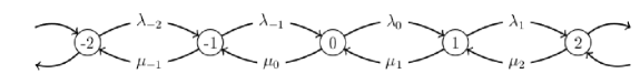
The transition diagram of is shown in the figure below666In order to keep the figure and the matrices readable, whenever it does not introduce any ambiguity,
the argument of the intensity functions is omitted..
Figure 1: Possible transitions for and corresponding intensities
Let and
.
For what follows it will be convenient to
write the Kolmogorov forward equations for the distribution of as777Special
cases of these well-known equations have been the starting point
for numerous papers; see, for example, early research on population dynamics in [37, Section 3].
(2)
where is the transposed generator
i.e. .
Since ,
the linear operator is bounded
and locally integrable for .
Thus (2) is the system of differential
equations in the space with the (bounded) linear operator.
And thus (see, for instance, [1])
it has the unique solution for
arbitrary initial conditions.
Moreover, if for some the
probabilities are all non-negative
for and ,
then the same holds for when .
What follows next relies on the concept of the logarithmic norm of
locally integrable operator functions
(see [1, 27]) and available from the literature
estimates for differential equations; detailed definitions and derivations
can be recovered from, for example, [16, Appendix].
3 Basic estimates
Theorem 1. Let there exist a doubly infinite sequence of positive numbers
such that and ,
where
and the function is given by
Then is weakly ergodic and
for all and any initial conditions and
it holds that
(3)
Proof.
Since ,
the Kolmogorov forward equations (2) for the distribution of
can be re-written as
(4)
where the vectors and are
and the linear transformation is given by the block matrix
which entries are itself matrices of the form
Denote by and
correspondingly the upper and
the lower triangular matrix of the form
Both of these matrices are known as semicirculant matrices.
Consider the linear transformation
given by the block matrix .
In what follows we will need the
inverse linear map of , which is further denoted by
. In order to show that it exists
for the considered matrix we will make use of the well-known
fact that the mapping of formal power series into the set
of infinite semicirculant matrices is an isomorphism.
Let us associate with the matrix
the formal power series
(we write ).
The values of are in the first bottom row of .
With the matrix we associate
the formal power series
(i.e. ).
The values of are in the first upper row of .
Consider the matrix . Since the mapping is an isomorphism,
then and ,
and thus then .
Note now that inverse matrix to , denote it by ,
exists since .
Denote the formal power series of
by .
Since ,
then (see [25, Theorem 1.2b]).
It is straightforward to check
that
and .
Thus we have
(5)
Both formal power series and have associated semicitculant matrices
Introduce the block matrix .
Thus we have .
But since ,
then ,
where is the identity matrix.
Thus is the left and right inverse linear map of .
Consider the similarity transformation ,
further denoted by . It is well-defined and given by the matrix
Note that unlike the matrix
all off-diagonal entries of are non-negative.
Choose an double infinite sequence
of positive numbers and
consider the linear transformation .
It is known (see [26, p. 19]) that
has a unique right-hand reciprocal,
which is the diagonal matrix .
It is straightforward to check, that the
linear transformation
is given by the matrix
which has only non-negative off-diagonal elements.
Coming back to (4), note that any
upper bound on the convergence rate
to the limiting regime for ,
corresponds to the same bound for
the solutions of the system
(6)
without the free term .
Here the vector and its elements can either positive or negative. Denote and . By left-multiplying both parts of (6) by , we get
(7)
where is, as well as , the vector
with the elements of arbitrary signs. Let us estimate the logarithmic norm of .
It is well-known that in the -norm
the logarithmic norm
of a (locally integrable) operator is equal to
(see, for example, [16, Appendix]).
By direct inspection it can be instantly seen that
the th column sum of is equal to
, where
Thus .
Let be such a doubly infinite sequence,
that
for . Denote .
Then
and thus is the bounded operator.
Now, if is the Cauchy operator of the equation (7), then
for any and
the following bound holds (for the justification see, for example, [16, Theorem A2]):
(8)
Now let and be such that
the corresponding and exist.
Then for any we have
∎
The inequality (3) holds even if .
This happens only if the intensities approach as becomes infinite
and thus the limiting ergodic distribution cannot not exist (cf. [32, Example 3]).
It is also worth noticing here that is not necessarily an
everywhere positive function.
Corollary 1. Assume that under the assumptions of the Theorem 1
there exist positive constants and such that
for any .
Then for any positive integer and all it holds that
Let us left-multiply the left and the right part
of the previous relation by . Using the estimates obtained
in the Theorem 1 and assuming that
there exist constants and such that
for any , we get
(11)
Indeed, .
Note that since all are positive, then for
any positive integer we have
From here we get two concentration inequalities for ,
which are valid for any integer :
Combining this with the upper bound for
we get for any positive integer :
∎
Note that since the bound in the Corollary 1
is valid for any , it is valid for the limiting probabilities
as well (if they exist).
One can simplify the bound (9) by fixing the initial condition.
For example, if , which implies that ,
then the first term in the brackets in the right hand-side of
(9) is zero.
Theorem 2. Let be a BDP on
for which the Corollary 1 holds. Let be its truncated version
with the state space ,
, . If there exist
constants , and ,
such that the Corollary 1 holds for , then
the following upper bound for the difference between the probability
distributions of and
(12)
holds for any if .
Proof. Consider the BDP with the state space
and the intensities if ,
and if
and other intensities equal to zero.
Thus the linear operator
is still given by the bi-infinite matrix.
The Kolmogorov forward equations for the distribution of
the , being the truncated ,
are
Then we have the following relations between the solutions of (4)
and (15):
(16)
where
For simplicity we assume further, that
(i.e. with the probability )
Then for any .
Next, it is clear that the first and the third terms in the (16)
are equal to zero and the difference
between and is just
(17)
Let
be an double infinite sequence
of positive numbers such that
there exist positive and such that
(18)
for any , where
and the functions is given by
By left-multiplying both parts of
(17) by the matrix ,
introduced abive,
and using the estimates obtained above we get:
(19)
Since for any , then
under the assumption that both BDPs start in the state, relations (17)
and (19)
imply the bound
Put . The following sequence
of inequalities completes the proof:
∎
The argumentation of the Theorem 2 allows one also to
obtain the upper bound for the truncation error, when computing
the average value given that initially the process
was in the state. Let .
Then
Using now the upper bound for
from the Theorem 2,
we get the upper bound for the .
In what follows we show,
how the developed theory can be used to
obtain explicit results.
4 Numerical examples
Two examples are considered in this section.
Their main purpose is to illustrate that the developed theory
indeed allows one to study numerically
arbitrary bilateral BDP with uniformly bounded
and state-dependent intensity functions.
Specific forms of the intensity functions
have been chosen for convenience of computation.
In each case it is assumed that .
In the first example we consider the randomized random walk on the integers,
say , which represents the position at time of a
particle moving along, say -axis, according to the following rules.
Its position can be shifted by at most to the right or left,
and it is assumed that these changes are
governed by the two Poisson processes with the time-varying parameters.
Specifically, when the particle is in a position
on the positive part of the -axis, it will move to
the position in
the infinitesimal time
with the probability
The next position
in the infinitesimal time
of the particle residing in the position
on the negative part of the
-axis is governed by the probability
.
If the particle enters the state then
its next state is or with the probability .
We make further simplifications. Let us assume that
.
Then when the particle is in the non-negative part
of the -axis, then
represents the number of customers
present in the classic queue
at epoch .
This example is somewhat artificial one and is due to [28].
From the Theorem 1 one can obtain the upper bound
for the rate of convergence, if a double infinite sequence,
say , can be found such that
.
Let us put and for , where .
Then we have:
(20)
Assume for now that there exists
such that .
Then and the upper bound follows from (3).
Further insight can be gained if one fixes exact values of , and .
So let us assume that , , . Then if one puts and for , then the constants
and from the Theorem 1 and Corollary 1 are equal to
and .
For the truncated process with the truncation threshold
one can put and for . Then the constants
and from the Theorem 2 are equal to and .
Thus, since
from (12) one gets
and from the comments, following the Theorem 2,
one obtains
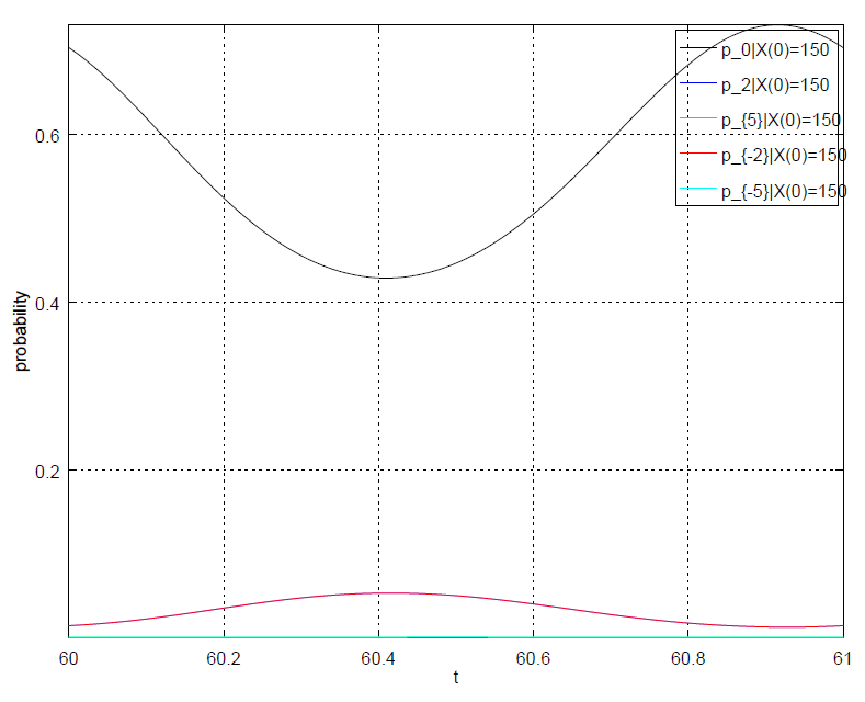
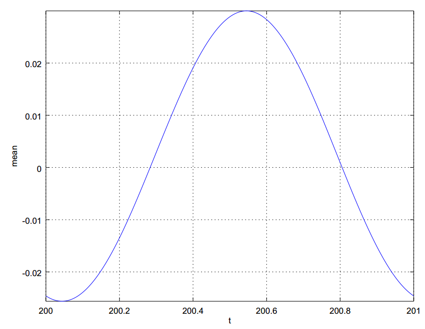
Figure 2: Limiting probability of particle position at time ,
showing variation with for given positions (.
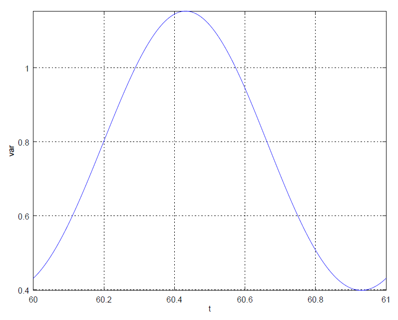
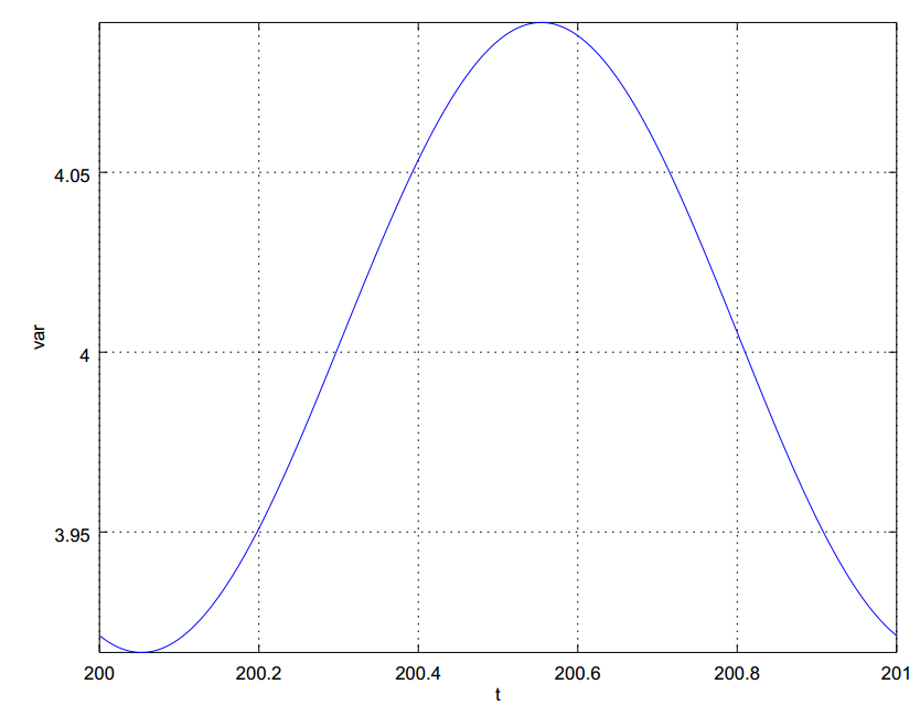
As expected in this example, the limiting average position fluctuates around 0, whereas the limiting variance is not (see Fig. 2). It
remains finite as the time becomes infinite.
Figure 3: Limiting variance of the particle position at time .
As the second example we consider the double-ended queueing system
with the state space .
Let be the queue length of taxi or passenger at time .
If , the number of passengers in the system is and
there is no taxi queue. If , the number of taxis in the system is and there is no passenger
queue. If , there is no taxi nor passenger.
Passengers and taxis arrive according to Poisson
process. Passengers (one to four passengers traveling together are considered as one passenger) arrive
to the queueing system according to a Poisson process with rate .
Obviously, is a one-dimensional continuous time
Markov chain.
The dynamic control of taxi depends on the state of the system.
If there is no passenger (i.e. ) waiting in the system,
the taxi arrival rate is , otherwise (i.e. ) the taxi arrival
rate is Obviously, the arrival rate of taxis with passengers is higher than that without passengers, i.e. .
Passengers and taxis match according to the first-in-first-out discipline
and matching is instantaneous.
The transposed intensity matrix for the considered problem
has the following structure:
The Theorem 1 yields the upper bound
for the convergence rate, if a double infinite sequence,
say , can be found such that
.
Let us put and for , where .
Then we have:
(21)
The value of cannot be written out
unless the exact values of and
are assumed. Let us fix
, and .
Then if one puts
,
and for , then the constants and from the Theorem 1 and Corollary 1 are equal to
and .
For the truncated process with the truncation threshold
one can put ,
and for .
Then the constants
and from the Theorem 2 are equal to and .
Thus, since
from (12) one gets
and from the comments, following the Theorem 2,
one obtains
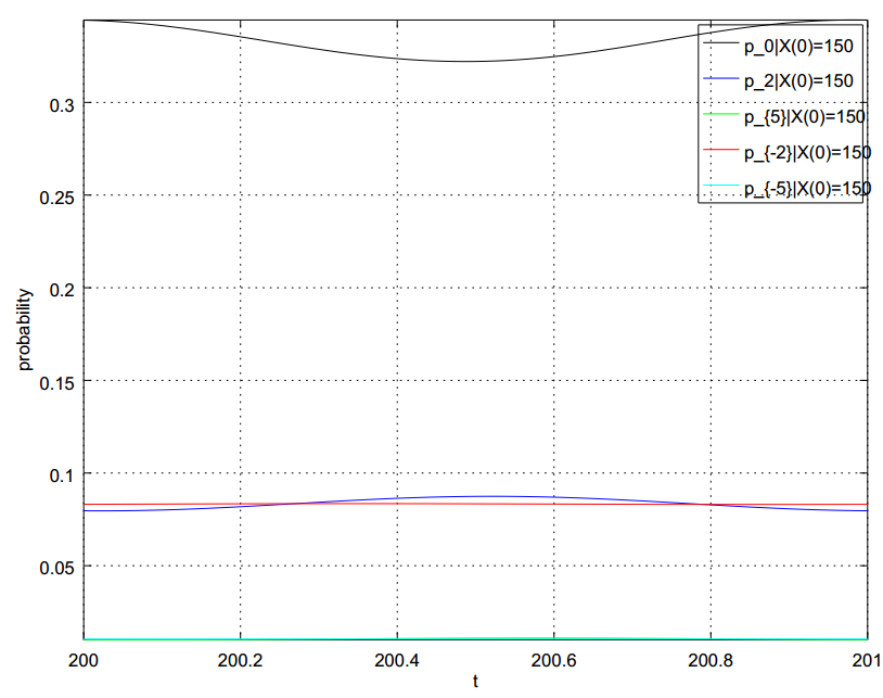
Fig. 3 shows the variation of with for
five different values .
Figure 4: Limiting probability of the process at time ,
showing variation with for given positions (.
In this example, as in the previous one,
the limiting average position fluctuates around 0
(see Fig. 4).
Figure 5: Limiting expected value of the process at time .
The limiting variance is not around zero (see Fig. 5)
and remains finite as the time becomes infinite.
Figure 6: Limiting variance of the process at time .
5 Conclusion
The developed theory for bilateral BDPs
facilitates their numerical analysis by providing upper
ergodicity and truncation bounds.
The latter can be used to understand when the limiting regime
is reached and show to properly truncate the
bi-infinite state space. The weak point of the
obtained results is the unknown bi-infinite sequence
of positive numbers , for which no rule of thumb can be suggested
and in each new use-case is has to be guessed.
Having no probabilistic meaning this sequence
can be considered as the analogue of Lyapunov functions.
Acknowledgements
This research was supported by Russian Science Foundation under grant 19-11-00020.
References
[1] Daleckij, Ju.L., Krein, M.G. (2002). Stability of solutions of
differential equations in Banach space. Amer. Math. Soc. Transl.
43.
[2] Di Crescenzo A., Nobile, A. G. (1995). Diffusion approximation to a queueing system with time dependent
arrival and service rates // Queueing Syst., 19, 41–62.
[3] E. A. Van Doorn, A. I. Zeifman, T. L. Panfilova
(2010). Bounds and asymptotics for the rate of convergence of
birth-death processes // Th. Prob. Appl., 54, 97–113.
[4]
Giorno, V., Nobile, A. G. (2019). First-passage times and related moments for continuous-time birth–death chains. Ricerche di Matematica, 68(2), 629–659.
[5] Giorno, V., Nobile, A. G. (2020). On a class of birth-death processes with time-varying intensity functions // Applied Mathematics and Computation, 379, 125255.
[6] B. L. Granovsky, A. I. Zeifman (2004). Nonstationary Queues:
Estimation of the Rate of Convergence // Queueing Syst. 46,
363–388.
[7] Knessl C. (2000). Exact and asymptotic solutions to a pde that arises in time-dependent
queues // Adv. Appl. Probab., 32, 256–283.
[8] Knessl C., Yang Y. P. (2002). An exact solution for an queue with time-dependent
arrivals and service // Adv. Appl. Probab., 40, 233–248.
[9] Mandelbaum A., Massey W. (1995). Strong approximations for time-dependent queues // Math.
Oper. Research, 20, 33–64.
[10] Masuyama, H. (2017). Continuous-time block-monotone Markov chains and their block-augmented truncations // Linear Algebra and its Applications, 514, 105–150.
[11] P. R. Parthasarathy, B. Krishna Kumar (1991). Density-dependent birth and death
processes with state-dependent immigration // Mathematical and
Computer Modelling, 15, 11–16.
[12] Satin Y. et al. Two-Sided Truncations For The Queueing Model //ECMS. – 2017. 635-641.
http://www.scs-europe.net/dlib/2017/2017-0635.htm
[13] Tweedie R. L. (1998). Truncation approximations of invariant measures for Markov chains // J. Appl. Probab., 35, 517–536.
[14] A. I. Zeifman (1982). Asymptotic behaviour of some stochastic models of species coexistence // Autom. Remote Control, 43:12, 1600–-1603
[15] Zeifman, A. I. (1989). Quasi-ergodicity for non-homogeneous continuous-time Markov chains // Journal of applied probability, 643–648.
[16] A. I. Zeifman (1995). Upper and lower bounds on the rate of
convergence for nonhomogeneous birth and death processes // Stoch.
Proc. Appl., 59, 157–173.
[17] Zeifman, A.I. (1988). Truncation error in a birth and
death system // USSR Computational Mathematics and Mathematical
Physics, 28(6), 210–211.
[18] A. Zeifman, S. Leorato, E. Orsingher, Ya. Satin, G.
Shilova (2006). Some universal limits for nonhomogeneous birth and
death processes // Queueing Syst., 52, 139–151.
[19] Zeifman A., Satin Y., Panfilova T. (2013). Limiting characteristics for
finite birth-death-catastrophe processes // Mathematical
biosciences, 245, 96–102.
[20] A. Zeifman, Ya. Satin, V. Korolev, S. Shorgin (2014). On truncations for weakly ergodic
inhomogeneous birth and death processes // International Journal of
Applied Mathematics and Computer Science, 24, 503–518.
[21] A. I. Zeifman, A. V. Korotysheva, V. Yu. Korolev, Ya. A. Satin (2017).
Truncation bounds for approximations of inhomogeneous
continuous-time Markov chains // Theory of Probability & Its Applications, 61(3), 513–520.
[22]
Zeifman, A., Satin, Y., Kovalev, I., Razumchik, R., & Korolev, V. (2021). Facilitating Numerical Solutions of Inhomogeneous Continuous Time Markov Chains Using Ergodicity Bounds Obtained with Logarithmic Norm Method. Mathematics, 9(1), 42.
[23]
Viswanath, N. C. (2020). Transient study of Markov models with time-dependent transition rates // Operational Research, 1-35.
[24]
Wang, Z., Yang, C., Liu, L., Zhao, Y. Q. (2021). Equilibrium and Socially optimal of a double-sided queueing system with two-mass point matching time. arXiv preprint arXiv:2101.12043.
[25]
P. Henrici, Applied and Computational Complex Analysis, Vol. 1, John Wiley & Sons, New
York, 1974.
[26]
R. G. Cooke, Infinite matrices and sequence spaces, London, 1950.
[27]
A. I. Zeifman (1995). On the Estimation of Probabilities for Birth and Death Processes //
Journal of Applied Probability, 32, 623–634.
[28] Conolly, B. W. (1971). On randomized random walks // SIAM Review, 13(1), 81–99.
[29] Liyanage, L. H., Gulati, C. M., Hill, J. M. (1982). A bibliography on applications of random walks in theoretical chemistry and physics // Advances in Molecular Relaxation and Interaction Processes, 22(1), 53–72.
[30]
Parthasarathy, P.R. and Lenin, R.B., Birth and death process (BDP) models with applications: queueing, com-
munication systems, chemical models, biological models: the state-of-the-art with a time-dependent perspective.
American Series in Mathematical and Management Sciences, vol. 51, American Sciences Press, Columbus, 2004.
[31] Kendall, D. G. (1951). Some problems in the theory of queues // Journal of the Royal Statistical Society: Series B (Methodological), 13(2), 151–173.
[32] Giveen, S. M. (1963). A taxicab problem with time-dependent arrival rates // SIAM Review, 5(2), 119–127.
[33] Wang, Z., Liu, L., Shao, Y., Chai, X., Chang, B. (2020). Equilibrium joining strategy in a batch transfer queuing system with gated policy // Methodology and Computing in Applied Probability, 22(1), 75–99.
[34] Pruitt, W. E. (1963). Bilateral birth and death processes // Transactions of the American Mathematical Society, 107(3), 508–525.
[35] Giorno, V., Nobile, A. G. (2019). First-passage times and related moments for continuous-time birth–death chains // Ricerche di Matematica, 68(2), 629–659.
[36] de la Iglesia, M. D. (2021). Spectral analysis of bilateral birth-death processes: some new explicit examples. arXiv preprint arXiv:2105.14419.
[37] Darwin, J. H. (1953). Population differences between species growing according to simple birth and death processes // Biometrika, 40(3/4), 370–382.
[38] Gibson, A. E., Conolly, B. W. (1971). On certain unrestricted, linear, unit step, continuous time random walks // Journal of Applied Probability, 8(2), 374–380.