A space-time multiscale mortar mixed finite element method for parabolic equations

Abstract

We develop a space-time mortar mixed finite element method for parabolic problems. The domain is decomposed into a union of subdomains discretized with non-matching spatial grids and asynchronous time steps. The method is based on a space-time variational formulation that couples mixed finite elements in space with discontinuous Galerkin in time. Continuity of flux (mass conservation) across space-time interfaces is imposed via a coarse-scale space-time mortar variable that approximates the primary variable. Uniqueness, existence, and stability, as well as a priori error estimates for the spatial and temporal errors are established. A space-time non-overlapping domain decomposition method is developed that reduces the global problem to a space-time coarse-scale mortar interface problem. Each interface iteration involves solving in parallel space-time subdomain problems. The spectral properties of the interface operator and the convergence of the interface iteration are analyzed. Numerical experiments are provided that illustrate the theoretical results and the flexibility of the method for modeling problems with features that are localized in space and time.

1 Introduction

The multiscale mortar mixed finite element method of [3, 5] allows for highly efficient and accurate discretization of elliptic problems. Let a spatial domain $\Omega$ be given, which is decomposed into subdomains ${\Omega}_{i}$. Then, on each ${\Omega}_{i}$, an individual mesh is set, and a standard mixed finite element scheme is considered. A stand-alone mortar variable approximating the primary variable is further introduced on an independent interface mesh, which is typically coarser but where one possibly employs polynomials of higher degree. It is used to couple the subdomain problems and to ensure (multiscale) weak continuity of the normal component of the mixed finite element flux variable over the interfaces between subdomains. Moreover, the mortar variable enables a very efficient parallelization in space via a non-overlapping domain decomposition algorithm based on reduction to an interface problem [3, 5, 28].

We introduce here a space-time discretization of a model parabolic equation, extending the above philosophy to time-dependent problems. Let a time interval $(0,T)$ be given. For each subdomain ${\Omega}_{i}$, our approach considers an individual space mesh of ${\Omega}_{i}$ along with individual time stepping on $(0,T)$. On each space-time subdomain ${\Omega}_{i}\times(0,T)$, any standard mixed finite element scheme is combined with the discontinuous Galerkin (DG) time discretization [50]. Then a stand-alone mortar variable approximating the primary variable is introduced on an independent space-time interface mesh, which is typically coarse and where higher polynomial degrees may be used. It is used to couple the space-time subdomain problems and to ensure (multiscale) weak continuity of the normal component of the mixed finite element flux variable (and consequently mass conservation) over the space-time interfaces. This setting allows for high flexibility with individual discretizations of each space-time subdomain $\Omega_{i}\times(0,T)$, and in particular for local time stepping. Moreover, space-time parallelization can be achieved via reduction to a space-time interface problem requiring the solution of discrete problems on the individual space-time subdomains $\Omega_{i}\times(0,T)$, exchanging space-time boundary data through transmission conditions, in the spirit of space-time domain decomposition methods as in, e.g., [33, 34, 25, 21, 51, 23, 10, 45, 32, 24].

We mention some of the related previous works on local time stepping for parabolic problems in mixed formulations. The early work [19] studies finite difference methods on grids with local refinement in space and time. A similar approach is employed in [16] for transport equations. Two space-time domain decomposition methods are considered in [33] – a space-time Steklov–Poincaré operator and optimized Schwarz waveform relaxation (OSWR) [23] with Robin transmission conditions. Asynchronous time stepping is allowed, but the spatial grids are assumed matching. The focus is on the analysis of the iterative convergence of the OSWR method. A posteriori error estimates for these methods are developed in [4, 2] for nested time grids, with [4] also allowing for non-matching spatial grids through the use of mortar finite elements. The methods from [33] a re extended to fracture modeling in [34]. Overlapping Schwarz domain decomposition with local grid refinement in space and time for two-phase flow in porous media is developed in [39]. Domain decomposition methods for mortar mixed finite element methods for parabolic problems with non-matching spatial grids and uniform time stepping are studied in [22, 6]. For parabolic problems in non-mixed form, domain decomposition methods with local time stepping have been studied, e.g., in [10, 45, 21, 51, 32, 24, 41, 15, 31]. Parallelism in time has also been explored, such as the Parareal algorithm [42, 27] and multigrid in time [20, 26]. Local time stepping techniques have been developed for multiphysics systems coupled through interface conditions, e.g., for the Stokes–Darcy system [35, 47]. Finally, we mention some earlier works on space-time methods for parabolic problems coupling mixed finite element discretizations in space with DG in time on a single domain. In [8], a method using continuous trial and discontinuous test functions in time is developed. A posteriori error estimation and space-time adaptivity for mixed finite element – DG methods is studied in [12, 40].

To the best of the authors’ knowledge, the solvability, stability, and a priori error analysis for space-time domain decomposition methods with non-matching spatial grids and asynchronous time stepping have not been studied in the literature, which is the main goal of this paper. A key tool in the analysis is the construction of an interpolant in a space-time weakly continuous velocity space, which is used to prove a discrete divergence inf-sup condition on this space. Another key component is establishing a discrete space-time mortar inf-sup condition under a suitable assumption on the mortar space. In addition to performing complete analysis in the general case, we also consider conforming time discretizations. In this case, we provide stability and error bounds for the velocity divergence and improved error estimates. To the best of our knowledge, such result has not been established in the literature for space-time mixed finite element methods with a DG time discretization, eve n on a single domain. Finally, we develop a parallel non-overlapping domain decomposition algorithm for the solution of the resulting algebraic problem. In particular, we utilize a time-dependent Steklov–Poincaré operator approach to reduce the global problem to a space-time interface problem. We show that the interface operator is positive definite and analyze its spectral properties. We employ an interface GMRES algorithm, which involves solving in parallel space-time subdomain problems at each iteration. The current iteration value of the mortar variable provides a Dirichlet boundary data on the space-time interfaces for the subdomain problems. We emphasize that, due to the discontinuous time discretization, the space-time subdomain problems are solved using classical time marching over the local time grid. We utilize the spectral bound of the interface operator to obtain an estimate for the number of interface GMRES iterations through field-of-values analysis.

This contribution is organized as follows. In Section 2, we describe the model problem and its domain decomposition weak formulation. Our space-time multiscale mortar discretization is introduced in Section 3, and we prove its existence, uniqueness, and stability with respect to data in Section 4. Section 5 derives a priori error estimates. Control of the velocity divergence and improved error estimates are established in Section 6. The reduction to a space-time interface problem and its analysis are presented in Section 7. We finally present numerical illustrations in Section 8 and close with conclusions in Section 9.

2 Setting

In this section we introduce the setting for our study.

2.1 Model problem

We consider a parabolic partial differential equation in a mixed form, modeling single phase flow in porous media. Let $\Omega\subset\mathbb{R}^{d}$, $d=2,3$, be a spatial polytopal domain with Lipschitz boundary and let $T>0$ be the final time. The governing equations are

$${\bf u}=-K\nabla p,\quad\frac{\partial p}{\partial t}+\nabla\cdot{\bf u}=q\quad\mbox{in }\Omega\times(0,T],$$ (2.1a)

where $$p {\bf u} q K$$ is the fluid pressure, is the Darcy velocity, is a source term, and is a tensor representing the rock permeability divided by the fluid viscosity. We assume for simplicity homogeneous Dirichlet boundary condition

$$p(x,t)=0\text{ on }\partial\Omega\times(0,T]$$ (2.1b)

and assign the initial pressure

$$p(x,0)=p_{0}(x)\text{ on }\Omega.$$ (2.1c)

We assume that $q\in L^{2}(0,T;L^{2}({\Omega}))$, $p_{0}\in H^{1}_{0}({\Omega})$, $\nabla\cdot K\nabla p_{0}\in L^{2}(\Omega)$, and that $K$ is a spatially-dependent, uniformly bounded, symmetric, and positive definite tensor, i.e., for constants $0<k_{\min}\leq k_{\max}<\infty$,

$$\text{ for a.e. }x\in{\Omega},\quad k_{\min}\zeta^{T}\zeta\leq\zeta^{T}K(x)\zeta\leq k_{\max}\zeta^{T}\zeta\quad\forall\zeta\in\mathbb{R}^{d},\ d=2,3.$$ (2.2)

Moreover, we suppose a scaling such that the diameter of ${\Omega}$ and the final time $T$ are of order one.

2.2 Space-time subdomains

Let $\Omega$ be a union of non-overlapping polytopal subdomains with Lipschitz boundary, $\overline{\Omega}=\cup\overline{\Omega}_{i}$. Let $\Gamma_{i}=\partial\Omega_{i}\setminus\partial\Omega$ be the interior boundary of $\Omega_{i}$, let $\Gamma_{ij}=\Gamma_{i}\cap\Gamma_{j}$ be the interface between two adjacent subdomains ${\Omega}_{i}$ and ${\Omega}_{j}$, and let $\Gamma=\cup\Gamma_{ij}$ be the union of all subdomain interfaces. We also introduce the space-time counterparts ${\Omega}^{T}={\Omega}\times(0,T)$, ${\Omega}_{i}^{T}={\Omega}_{i}\times(0,T)$, $\Gamma_{i}^{T}=\Gamma_{i}\times(0,T)$, and $\Gamma_{ij}^{T}=\Gamma_{ij}\times(0,T)$. We will introduce space-time domain decomposition discretizations based on ${\Omega}_{i}^{T}$.

2.3 Basic notation

We will utilize the following notation. For a domain ${\cal O}\subset\mathbb{R}^{d}$, the $L^{2}({\cal O})$ inner product and norm for scalar and vector-valued functions are denoted by $(\cdot,\cdot)_{{\cal O}}$ and $\|\cdot\|_{{\cal O}}$, respectively. The norms and seminorms of the Sobolev spaces $W^{k,p}({\cal O}),\,k\in\mathbb{R},p\geq 1$, are denoted by $\|\cdot\|_{k,p,{\cal O}}$ and $|\cdot|_{k,p,{\cal O}}$, respectively. The norms and seminorms of the Hilbert spaces $H^{k}({\cal O})$ are denoted by $\|\cdot\|_{k,{\cal O}}$ and $|\cdot|_{k,{\cal O}}$, respectively. For a section of a subdomain boundary $S\subset\mathbb{R}^{d-1}$ we write $\langle\cdot,\cdot\rangle_{S}$ and $\|\cdot\|_{S}$ for the $L^{2}(S)$ inner product (or duality pairing) and norm, respectively. By ${\bf M}$ we denote the vectorial counterpart of a generic scalar space $M$.

The above notation is extended to space-time domains as follows. For ${\cal O}^{T}={\cal O}\times(0,T)$ and $S^{T}=S\times(0,T)$, let $(\cdot,\cdot)_{{\cal O}^{T}}=\int_{0}^{T}(\cdot,\cdot)_{{\cal O}}$ and $\langle\cdot,\cdot\rangle_{S^{T}}=\int_{0}^{T}\langle\cdot,\cdot\rangle_{S}$. For space-time norms we use the standard Bochner notation. For example, given a spatial norm $\|\cdot\|_{V}$, we denote, for $p>0$,

$$\|\cdot\|_{L^{p}(0,T;V)}=\left(\int_{0}^{T}\|\cdot\|_{V}^{p}\right)^{\frac{1}{p}},\quad\|\cdot\|_{L^{\infty}(0,T;V)}=\text{ess}\sup\|\cdot\|_{V},$$

with the usual extension for $\|\cdot\|_{W^{k,p}(0,T;V)}$ and $\|\cdot\|_{H^{k}(0,T;V)}$. Let $\|\cdot\|_{S^{T}}=\|\cdot\|_{L^{2}(0,T;L^{2}(S))}$. We will use the space

$${\bf H}({\rm div};{\cal O})=\left\{{\bf v}\in{\bf L}^{2}({\cal O}):\nabla\cdot{\bf v}\in L^{2}({\cal O})\right\},$$

equipped with the norm

$$\|{\bf v}\|_{{\rm div};{\cal O}}=\left(\|{\bf v}\|_{{\cal O}}^{2}+\|\nabla\cdot{\bf v}\|_{{\cal O}}^{2}\right)^{\frac{1}{2}}.$$

Finally, throughout the paper, $C$ will denote a generic constant that is independent of the spatial and temporal discretization parameters.

2.4 Weak formulation

The weak formulation of problem (2.1) reads: find $({\bf u},p):[0,T]\mapsto{\bf H}({\rm div};{\Omega})\times L^{2}({\Omega})$ such that $p(x,0)=p_{0}$ and for a.e. $t\in(0,T)$,

$$(K^{-1}{\bf u},{\bf v})_{\Omega}-(p,\nabla\cdot{\bf v})_{\Omega}=0\quad\forall\,{\bf v}\in{\bf H}({\rm div};{\Omega}),$$ (2.3a)

$$(\partial_{t}p,w)_{\Omega}+(\nabla\cdot{\bf u},w)_{\Omega}=(q,w)_{\Omega}\quad\forall\,w\in L^{2}({\Omega}).$$ (2.3b)

The following well-posedness result is rather standard and presented in, e.g., [33, Theorem 2.1].

Theorem 2.1 (Well-posedness).

Problem (2.3) has a unique solution ${\bf u}\in L^{2}(0,T;{\bf H}({\rm div};{\Omega}))\cap L^{\infty}(0,T;{\bf L}^{2}(\Omega))$, $p\in H^{1}(0,T;H_{0}^{1}({\Omega}))$.

We note that in particular the inclusion $p\in H^{1}(0,T;H_{0}^{1}({\Omega}))$ follows from (2.3a), which implies that for a.e. $t\in(0,T)$, $\nabla p=-K^{-1}{\bf u}$ in the sense of distributions.

2.5 Domain decomposition weak formulation

We now give a domain decomposition weak formulation of (2.3). Introduce the subdomain velocity and pressure spaces

$${\bf V}_{i}={\bf H}({\rm div};{\Omega}_{i}),\,\,{\bf V}=\bigoplus{\bf V}_{i},\quad W_{i}=L^{2}({\Omega}_{i}),\,\,W=\bigoplus W_{i}=L^{2}({\Omega}),$$

endowed with the norms

$$\|{\bf v}\|_{{\bf V}_{i}}=\|{\bf v}\|_{{\rm div};{\Omega}_{i}},\quad\|{\bf v}\|_{{\bf V}}=\left(\sum_{i}\|{\bf v}\|_{{\bf V}_{i}}^{2}\right)^{\frac{1}{2}},\quad\|w\|_{W}=\|w\|_{\Omega}.$$

We also introduce the following spatial bilinear forms, which will prove useful below:

$$a_{i}({\bf u},{\bf v})=(K^{-1}{\bf u},{\bf v})_{\Omega_{i}},\quad a({\bf u},{\bf v})=\sum_{i}a_{i}({\bf u},{\bf v}),$$ (2.4a)

$$b_{i}({\bf v},w)=-(\nabla\cdot{\bf v},w)_{\Omega_{i}},\quad b({\bf v},w)=\sum_{i}b_{i}({\bf v},w),$$ (2.4b)

$$b_{\Gamma}({\bf v},\mu)=\sum_{i}\langle{\bf v}\cdot{\bf n}_{i},\mu\rangle_{\Gamma_{i}}.$$ (2.4c)

In addition, for any spatial bilinear form $s(\cdot,\cdot)$, let $\displaystyle s^{T}(\cdot,\cdot)=\int_{0}^{T}s(\cdot,\cdot)$.

Now, since $p\in H^{1}(0,T;H_{0}^{1}({\Omega}))$, we can consider the trace of the pressure $p$ on the interfaces, $\lambda=p|_{\Gamma}$. Thus, integrating in time, it is easy to see that the solution $({\bf u},p)$ of (2.3) satisfies

$$a^{T}({\bf u},{\bf v})+b^{T}({\bf v},p)+b^{T}_{\Gamma}({\bf v},\lambda)=0\quad\forall\,{\bf v}\in L^{2}(0,T;{\bf V}),$$ (2.5a)

$$(\partial_{t}p,w)_{\Omega^{T}}-b^{T}({\bf u},w)=(q,w)_{\Omega^{T}}\quad\forall\,w\in L^{2}(0,T;W).$$ (2.5b)

3 Space-time mortar mixed finite element method

We consider a space-time discretization of (2.5), motivated by [33]. It employs a mortar finite element variable to approximate the pressure trace $\lambda$ from (2.5) and uses it as a Lagrange multiplier to impose weakly the continuity of flux across space-time interfaces.

3.1 Space-time grids and spaces

Let ${\cal T}_{h,i}$ be a shape-regular partition of the subdomain $\Omega_{i}$ into parallelepipeds or simplices in the sense of [13]. We stress that this allows for grids that do not match along the interfaces $\Gamma_{ij}$ between subdomains $\Omega_{i}$ and $\Omega_{j}$. Let $h_{i}=\max_{E\in{\cal T}_{h,i}}\text{diam}\,E$ and $h=\max_{i}h_{i}$. In some parts of the analysis, we will additionally require ${\cal T}_{h,i}$ to be quasi-uniform in that $h_{i}\leq C\text{diam}\,E\ \forall E\in{\cal T}_{h,i}$, as well as that the mesh sizes in all subdomains be comparable in that $h\leq Ch_{i}\ \forall i$. Similarly, let ${\cal T}^{\Delta t}_{i}:0=t_{i}^{0}<t_{i}^{1}<\cdots<t_{i}^{N_{i}}=T$ be a partition of the time interval $(0,T)$ corresponding to subdomain $\Omega_{i}$. This means that we consider different time discretizations on different subdomains. Let ${\Delta t}_{i}=\max_{1\leq k\leq N_{i}}|t_{i}^{k}-t_{i}^{k-1}|$ and ${\Delta t}=\max_{i}{\Delta t}_{i}$. Though we admit non-uniform time stepping, we will sometimes require that ${\cal T}^{\Delta t}_{i}$ be quasi-uniform in that ${\Delta t}_{i}\leq C|t_{i}^{k}-t_{i}^{k-1}|\ \forall(t_{i}^{k-1},t_{i}^{k})\in{\cal T}^{\Delta t}_{i}$, as well as that the time steps in all subdomains be comparable in that ${\Delta t}\leq C{\Delta t}_{i}\ \forall i$.

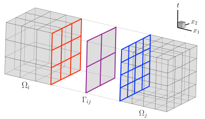
Figure 1: Non-matching space-time subdomain and mortar grids in two spatial dimensions.

Composing ${\cal T}_{h,i}$ and ${\cal T}^{\Delta t}_{i}$ by tensor product results in a space-time partition

$${\cal T}^{\Delta t}_{h,i}={\cal T}_{h,i}\times{\cal T}^{\Delta t}_{i}$$

of the space-time subdomain $\Omega_{i}^{T}$. An illustration is given in Figure 1, where yet a different, mortar space-time grid, is also shown in the middle.

For discretization in space, we consider any of the inf–sup stable mixed finite element spaces ${\bf V}_{h,i}\times W_{h,i}\subset{\bf V}_{i}\times W_{i}$ such as the Raviart–Thomas or the Brezzi–Douglas–Marini spaces, see, e.g., [11]. For discretization in time, we will in turn utilize the discontinuous Galerkin (DG) method, cf. [50], which is based on a discontinuous piecewise polynomial approximation of the solution on the mesh ${\cal T}^{\Delta t}_{i}$. Denote by $W_{i}^{\Delta t}$ the subdomain time discretizations of the velocity and pressure. Composing the space and time discretizations

$${\bf V}_{h,i}^{\Delta t}={\bf V}_{h,i}\times W_{i}^{\Delta t},\quad W_{h,i}^{\Delta t}=W_{h,i}\times W_{i}^{\Delta t}$$

results in the space-time mixed finite element spaces ${\bf V}_{h,i}^{\Delta t}\times W_{h,i}^{\Delta t}$ in each space-time subdomain $\Omega_{i}^{T}$. We will also need the spatial variable only spaces

$${\bf V}_{h}=\bigoplus{\bf V}_{h,i},\quad W_{h}=\bigoplus W_{h,i}.$$

Let ${\cal T}_{H,ij}$ be a shape-regular finite element partition of $\Gamma_{ij}$, where $H=\max_{i,j}\max_{e\in{\cal T}_{H,ij}}\text{diam}\,e$, see Figure 1, middle. The use of index $H$ indicates a possibly coarser interface grid compared to the subdomain grids, resulting in a multiscale approximation. Let ${\cal T}^{\Delta T}_{ij}:0=t_{ij}^{0}<t_{ij}^{1}<\cdots<t_{ij}^{N_{ij}}=T$ be a partition of $(0,T)$ corresponding to $\Gamma_{ij}$, which may be different from (and again possibly coarser than) the time-partitions for the neighboring subdomains. Let $\Delta T=\max_{i,j}\max_{1\leq k\leq N_{ij}}|t_{ij}^{k}-t_{ij}^{k-1}|$. Composing ${\cal T}_{H,ij}$ and ${\cal T}^{\Delta T}_{ij}$ by tensor product gives a space-time partition

$${\cal T}^{\Delta T}_{H,ij}={\cal T}_{H,ij}\times{\cal T}^{\Delta T}_{ij}$$

of the space-time interface $\Gamma_{ij}^{T}$. Finally, let

$$\Lambda_{H,ij}^{\Delta T}=\Lambda_{H,ij}\times\Lambda_{ij}^{\Delta T}$$

be a space-time mortar finite element space on ${\cal T}^{\Delta T}_{H,ij}$ consisting of continuous or discontinuous piecewise polynomials in space and in time. We will also need the spatial variable only space

$$\Lambda_{H}=\bigoplus\Lambda_{H,ij}.$$

Finally, the global space-time finite element spaces are defined as

$${\bf V}_{h}^{\Delta t}=\bigoplus{\bf V}_{h,i}^{\Delta t},\quad W_{h}^{\Delta t}=\bigoplus W_{h,i}^{\Delta t},\quad\Lambda_{H}^{\Delta T}=\bigoplus\Lambda_{H,ij}^{\Delta T}.$$ (3.1)

In particular, the Lagrange multiplier will be sought for in the mortar space $\Lambda_{H}^{\Delta T}$. For the purpose of the analysis, we also define the space of velocities with space-time weakly continuous normal components

$${\bf V}_{h,0}^{\Delta t}=\left\{{\bf v}\in{\bf V}_{h}^{\Delta t}:b^{T}_{\Gamma}({\bf v},\mu)=0\quad\forall\,\mu\in\Lambda_{H}^{\Delta T}\right\}.$$ (3.2)

The discrete velocity and pressure spaces inherit the norms $\|\cdot\|_{{\bf V}}$ and $\|\cdot\|_{W}$, respectively. The mortar space is equipped with the spatial norm $\|\mu\|_{\Lambda_{H}}=\|\mu\|_{L^{2}(\Gamma)}$.

3.2 Space-time multiscale mortar mixed finite element method

For the DG time discretization, we introduce the notation for $\varphi(x,\cdot)$, $\phi(x,\cdot)\in W_{i}^{\Delta t}$, $x\in\Omega_{i}$, see [50],

$$\int_{0}^{T}\tilde{\partial}_{t}\varphi\,\phi=\sum_{k=1}^{N_{i}}\int_{t_{i}^{k-1}}^{t_{i}^{k}}\partial_{t}\varphi\,\phi+\sum_{k=1}^{N_{i}}[\varphi]_{k-1}\,\phi_{k-1}^{+},$$ (3.3)

where $[\varphi]_{k}=\varphi_{k}^{+}-\varphi_{k}^{-}$, with $\varphi_{k}^{+}=\lim_{t\to t_{i}^{k,+}}\,\varphi$ and $\varphi_{k}^{-}=\lim_{t\to t_{i}^{k,-}}\,\varphi$.

Remark 3.1 (Initial value).

In what follows, we will tacitly assume that a function $\varphi(x,\cdot)\in W_{i}^{\Delta t}$ has an associated initial value $\varphi_{0}^{-}$, which will be defined if it is explicitly used.

The space-time multiscale mortar mixed finite element method for approximating (2.5) is: find ${\bf u}_{h}^{\Delta t}\in{\bf V}_{h}^{\Delta t}$, $p_{h}^{\Delta t}\in W_{h}^{\Delta t}$, and $\lambda_{H}^{\Delta T}\in\Lambda_{H}^{\Delta T}$ such that

$$a^{T}({\bf u}_{h}^{\Delta t},{\bf v})+b^{T}({\bf v},p_{h}^{\Delta t})+b^{T}_{\Gamma}({\bf v},\lambda_{H}^{\Delta T})=0\quad\forall\,{\bf v}\in{\bf V}_{h}^{\Delta t},$$ (3.4a)

$$(\tilde{\partial}_{t}p_{h}^{\Delta t},w)_{\Omega^{T}}-b^{T}({\bf u}_{h}^{\Delta t},w)=(q,w)_{\Omega^{T}}\quad\forall\,w\in W_{h}^{\Delta t},$$ (3.4b)

$$b^{T}_{\Gamma}({\bf u}_{h}^{\Delta t},\mu)=0\quad\forall\,\mu\in\Lambda_{H}^{\Delta T},$$ (3.4c)

where the obvious notation $(\tilde{\partial}_{t}p_{h}^{\Delta t},w)_{\Omega^{T}}=\sum_{i}(\tilde{\partial}_{t}p_{h}^{\Delta t},w)_{\Omega_{i}^{T}}$ has been used. We note that $(\tilde{\partial}_{t}p_{h}^{\Delta t},w)_{\Omega^{T}}$ involves the term $\big{(}(p_{h}^{\Delta t})_{0}^{+}-(p_{h}^{\Delta t})_{0}^{-},w_{0}^{+}\big{)}_{\Omega}$, see the last term in (3.3) for $k=1$. Here, $(p_{h}^{\Delta t})_{0}^{+}$ is computed by the method, while $(p_{h}^{\Delta t})_{0}^{-}$ is determined by the initial condition. We discuss the construction of initial data in Section 4.4.

The above method provides a highly general and flexible framework, allowing for different spatial and temporal discretizations in different subdomains. We note that according to (3.4c), continuity of the flux is imposed weakly on the space-time interfaces $\Gamma_{ij}^{T}$, requiring that the jump in flux is orthogonal to the space-time mortar space $\Lambda_{H,ij}^{\Delta T}$. This formulation results in a correct notion of mass conservation across interfaces for time-dependent domain decomposition problems with non-matching grids in both space and time. In the case of discontinuous mortars, (3.4c) implies that the total flux across any space-time interface cell $e\times(t_{ij}^{k-1},t_{ij}^{k})$, $e\in{\cal T}_{H,ij}$, is continuous.

4 Well-posedness analysis

In this section we analyze the existence, uniqueness, and stability of the solution to (3.4).

4.1 Space-time interpolants

We will make use of several space-time interpolants. Let ${\cal P}_{h,i}$ be the $L^{2}$-orthogonal projection onto $W_{h,i}$ and let ${\cal P}_{i}^{\Delta t}$ be the $L^{2}$-orthogonal projection onto $W_{i}^{\Delta t}$. We then define the $L^{2}$-orthogonal projection in space and time on subdomain $\Omega_{i}$ by

$${\cal P}_{h,i}^{\Delta t}={\cal P}_{h,i}\times{\cal P}_{i}^{\Delta t}:L^{2}(0,T;L^{2}(\Omega_{i}))\to W_{h,i}^{\Delta t}$$

and globally by

$${\cal P}_{h}^{\Delta t}:L^{2}(0,T;L^{2}(\Omega))\to W_{h}^{\Delta t},\quad{\cal P}_{h}^{\Delta t}|_{\Omega_{i}}={\cal P}_{h,i}^{\Delta t}.$$

Setting ${\cal P}_{h}|_{\Omega_{i}}={\cal P}_{h,i}$ and ${\cal P}^{\Delta t}|_{\Omega_{i}}={\cal P}_{i}^{\Delta t}$, we will also write ${\cal P}_{h}^{\Delta t}={\cal P}_{h}\times{\cal P}^{\Delta t}$. Since $\nabla\cdot{\bf V}_{h,i}=W_{h,i}$, we have, for all $\varphi\in L^{2}(0,T;L^{2}(\Omega_{i}))$,

$$({\cal P}_{h}^{\Delta t}\varphi-\varphi,\nabla\cdot{\bf v})_{{\Omega}_{i}^{T}}=0\quad\forall\,{\bf v}\in{\bf V}_{h,i}^{\Delta t}.$$ (4.1)

For $\epsilon>0$, denote ${\bf H}^{\epsilon}({\rm div};\Omega_{i}):={\bf H}^{\epsilon}(\Omega_{i})\cap{\bf H}({\rm div};\Omega_{i})$. Let $\boldsymbol{\Pi}_{h,i}:{\bf H}^{\epsilon}({\rm div};\Omega_{i})\to{\bf V}_{h,i}$ be the canonical mixed interpolant [11] and let

$$\boldsymbol{\Pi}_{h,i}^{\Delta t}=\boldsymbol{\Pi}_{h,i}\times{\cal P}_{i}^{\Delta t}:L^{2}(0,T;{\bf H}^{\epsilon}({\rm div};\Omega_{i}))\to{\bf V}_{h,i}^{\Delta t}.$$

In particular, this space-time interpolant satisfies, for all $\boldsymbol{\psi}\in L^{2}(0,T;{\bf H}^{\epsilon}({\rm div};\Omega_{i}))$,

$$(\nabla\cdot(\boldsymbol{\Pi}_{h,i}^{\Delta t}\boldsymbol{\psi}-\boldsymbol{\psi}),w)_{\Omega_{i}^{T}}=0\quad\forall\,w\in W_{h,i}^{\Delta t},$$ (4.2a)

$$\langle(\boldsymbol{\Pi}_{h,i}^{\Delta t}\boldsymbol{\psi}-\boldsymbol{\psi})\cdot{\bf n}_{i},{\bf v}\cdot{\bf n}_{i}\rangle_{\partial\Omega_{i}^{T}}=0\quad\forall\,{\bf v}\in{\bf V}_{h,i}^{\Delta t},$$ (4.2b)

$$\|\boldsymbol{\Pi}_{h,i}^{\Delta t}\boldsymbol{\psi}\|_{L^{2}(0,T;{\bf V}_{i})}\leq C(\|\boldsymbol{\psi}\|_{L^{2}(0,T;{\bf H}^{\epsilon}(\Omega_{i}))}+\|\nabla\cdot\boldsymbol{\psi}\|_{L^{2}(0,T;L^{2}(\Omega_{i}))}).$$ (4.2c)

Let ${\cal Q}_{h,i}:L^{2}(\partial\Omega_{i})\to{\bf V}_{h,i}\cdot{\bf n}_{i}$ be the $L^{2}$-orthogonal projection and let

$${\cal Q}_{h,i}^{\Delta t}={\cal Q}_{h,i}\times{\cal P}_{i}^{\Delta t}:L^{2}(0,T;L^{2}(\partial\Omega_{i}))\to{\bf V}_{h,i}^{\Delta t}\cdot{\bf n}_{i}.$$ (4.3)

Finally, let ${\cal P}_{H,\Gamma_{ij}}:L^{2}(\Gamma_{ij})\to\Lambda_{H,ij}$ and ${\cal P}_{ij}^{\Delta T}:L^{2}(0,T)\to\Lambda_{ij}^{\Delta T}$ be the $L^{2}$-orthogonal projections and let

$${\cal P}_{H,\Gamma_{ij}}^{\Delta T}={\cal P}_{H,\Gamma_{ij}}\times{\cal P}_{ij}^{\Delta T}:L^{2}(0,T;L^{2}(\Gamma_{ij}))\to\Lambda_{H,ij}^{\Delta T},\quad{\cal P}_{H,\Gamma}^{\Delta T}|_{\Gamma_{ij}}={\cal P}_{H,\Gamma_{ij}}^{\Delta T}$$ (4.4)

be the mortar space-time $L^{2}$-orthogonal projection.

4.2 Assumptions on the mortar grids

We make the following assumptions on the mortar grids, which are needed to guarantee that the method (3.4) is well posed: there exists a positive constant $C$ independent of the spatial mesh sizes $h$ and $H$ (as well as of the temporal mesh sizes ${\Delta t}$ and $\Delta T$) such that

$$\forall\,\mu\in\Lambda_{H},\ \forall\,i,j,\quad\|\mu\|_{\Gamma_{ij}}\leq C(\|{\cal Q}_{h,i}\,\mu\|_{\Gamma_{ij}}+\|{\cal Q}_{h,j}\,\mu\|_{\Gamma_{ij}}),$$ (4.5a)

$$\forall\,i,j,\quad\Lambda_{ij}^{\Delta T}\subset W_{i}^{\Delta t}\cap W_{j}^{\Delta t}.$$ (4.5b)

The spatial mortar assumption (4.5a) is the same as the assumption made in [3, 5]. Note that it is in particular satisfied with $C=\frac{1}{2}$ when ${\cal T}_{H,ij}$ is a coarsening of both ${\cal T}_{h,i}$ and ${\cal T}_{h,j}$ on the interface $\Gamma_{ij}$ and the space $\Lambda_{H,ij}$ consists of discontinuous piecewise polynomials contained in ${\bf V}_{h,i}\cdot{\bf n}_{i}$ and ${\bf V}_{h,j}\cdot{\bf n}_{j}$ on $\Gamma_{ij}$. In general, it requires that the mortar space $\Lambda_{H}$ is sufficiently coarse, so that it is controlled by the normal traces of the neighboring subdomain velocity spaces.

The temporal mortar assumption (4.5b) similarly provides control of the mortar time discretization by the subdomain time discretizations. It requires that each subdomain time discretization be a refinement of the mortar time discretization. We also note that (4.5a) and (4.5b) imply

$$\forall\,\mu\in\Lambda_{H}^{\Delta T},\forall\,i,j,\quad\|\mu\|_{L^{2}(0,T;L^{2}(\Gamma_{ij}))}\leq C(\|{\cal Q}_{h,i}^{\Delta t}\,\mu\|_{L^{2}(0,T;L^{2}(\Gamma_{ij}))}+\|{\cal Q}_{h,j}^{\Delta t}\,\mu\|_{L^{2}(0,T;L^{2}(\Gamma_{ij}))})$$ (4.6)

for a constant $C$ independent of $h$, $H$, ${\Delta t}$, and $\Delta T$.

4.3 Discrete inf–sup conditions

Recall the form $b^{T}(\cdot,\cdot)$ from (2.4b). Under the above assumptions on the mortar grids, the weakly continuous velocity space ${\bf V}_{h,0}^{\Delta t}$ of (3.2) satisfies the following inf–sup condition.

Lemma 4.1 (Discrete divergence inf–sup condition on ${\bf V}_{h,0}^{\Delta t}$).

Let (4.5) hold. Then there exists a constant $\beta>0$, independent of $h$, $H$, ${\Delta t}$, and $\Delta T$, such that

$$\forall\,w\in W_{h}^{\Delta t},\quad\sup_{0\neq{\bf v}\in{\bf V}_{h,0}^{\Delta t}}\frac{b^{T}({\bf v},w)}{\|{\bf v}\|_{L^{2}(0,T;{\bf V})}}\geq\beta\|w\|_{L^{2}(0,T;L^{2}({\Omega}))}.$$ (4.7)

Proof.

Let ${\bf V}_{h,0}=\left\{{\bf v}\in{\bf V}_{h}:b_{\Gamma}({\bf v},\mu)=0\quad\forall\,\mu\in\Lambda_{H}\right\}$. It is shown in [3, 5] that if (4.5a) holds, then there is an interpolant $\boldsymbol{\Pi}_{h,0}:{\bf H}^{\frac{1}{2}+\epsilon}({\rm div};\Omega)\to{\bf V}_{h,0}$ such that, for all $\boldsymbol{\psi}\in{\bf H}^{\frac{1}{2}+\epsilon}({\rm div};\Omega)$,

$$\sum_{i}(\nabla\cdot(\boldsymbol{\Pi}_{h,0}\boldsymbol{\psi}-\boldsymbol{\psi}),w)_{\Omega_{i}}=0\quad\forall\,w\in W_{h},$$ (4.8a)

$$\|\boldsymbol{\Pi}_{h,0}\boldsymbol{\psi}\|_{{\bf V}}\leq C(\|\boldsymbol{\psi}\|_{{\bf H}^{\frac{1}{2}+\epsilon}(\Omega)}+\|\nabla\cdot\boldsymbol{\psi}\|_{L^{2}(\Omega)}),$$ (4.8b)

for a constant $C$ independent of $h$ and $H$. Define

$$\boldsymbol{\Pi}_{h,0}^{\Delta t}=\boldsymbol{\Pi}_{h,0}\times{\cal P}^{\Delta t}.$$

We claim that $\boldsymbol{\Pi}_{h,0}^{\Delta t}:L^{2}(0,T;{\bf H}^{\frac{1}{2}+\epsilon}({\rm div};\Omega))\to{\bf V}_{h,0}^{\Delta t}$. To see this, note first that, for all functions $\boldsymbol{\psi}\in L^{2}(0,T;{\bf H}^{\frac{1}{2}+\epsilon}({\rm div};\Omega))$, clearly $\boldsymbol{\Pi}_{h,0}^{\Delta t}\boldsymbol{\psi}\in{\bf V}_{h}^{\Delta t}$. Thus (4.5b) implies

$$b^{T}_{\Gamma}(\boldsymbol{\Pi}_{h,0}^{\Delta t}\boldsymbol{\psi},\mu) =\sum_{i}\int_{0}^{T}\langle\boldsymbol{\Pi}_{h,0}^{\Delta t}\boldsymbol{\psi}\cdot{\bf n}_{i},\mu\rangle_{\Gamma_{i}}=\sum_{i}\int_{0}^{T}\langle\boldsymbol{\Pi}_{h,0}\boldsymbol{\psi}\cdot{\bf n}_{i},\mu\rangle_{\Gamma_{i}}$$

$$=\int_{0}^{T}b_{\Gamma}(\boldsymbol{\Pi}_{h,0}\boldsymbol{\psi},\mu)=0\quad\forall\,\mu\in\Lambda_{H}^{\Delta T},$$

i.e., indeed $\boldsymbol{\Pi}_{h,0}^{\Delta t}\boldsymbol{\psi}\in{\bf V}_{h,0}^{\Delta t}$ by virtue of (3.2). Moreover, (4.8a) and (4.8b) imply

$$\sum_{i}(\nabla\cdot(\boldsymbol{\Pi}_{h,0}^{\Delta t}\boldsymbol{\psi}-\boldsymbol{\psi}),w)_{\Omega_{i}^{T}}=0\quad\forall\,w\in W_{h}^{\Delta t},$$ (4.9a)

$$\|\boldsymbol{\Pi}_{h,0}^{\Delta t}\boldsymbol{\psi}\|_{L^{2}(0,T;{\bf V})}\leq C(\|\boldsymbol{\psi}\|_{L^{2}(0,T;{\bf H}^{\frac{1}{2}+\epsilon}(\Omega))}+\|\nabla\cdot\boldsymbol{\psi}\|_{L^{2}(0,T;L^{2}(\Omega))}).$$ (4.9b)

The inf–sup condition (4.7) then follows from the classical continuous inf–sup condition for $b^{T}(\cdot,\cdot)$, the existence of the interpolant $\boldsymbol{\Pi}_{h,0}^{\Delta t}$, and Fortin’s lemma [11]. ∎

To control the mortar variable, we need the following mortar inf–sup condition.

Lemma 4.2 (Discrete mortar inf–sup condition on ${\bf V}_{h}^{\Delta t}$).

Let (4.6) hold. Then there exists a constant $\beta_{\Gamma}>0$, independent of $h$, $H$, ${\Delta t}$, and $\Delta T$, such that

$$\forall\,\mu\in\Lambda_{H}^{\Delta T},\quad\sup_{0\neq{\bf v}\in{\bf V}_{h}^{\Delta t}}\frac{b^{T}_{\Gamma}({\bf v},\mu)}{\|{\bf v}\|_{L^{2}(0,T;{\bf V})}}\geq\beta_{\Gamma}\|\mu\|_{L^{2}(0,T;L^{2}(\Gamma))}.$$ (4.10)

Proof.

Let $\mu\in\Lambda_{H}^{\Delta T}$ be given. In the following we assume that $\mu$ is extended by zero on $\partial\Omega$. We consider a set of auxiliary subdomain problems. Let $\varphi_{i}(x,t)$ be the solution for a.e. $t\in(0,T)$ of the problem

$$\nabla\cdot\nabla\varphi_{i}(\cdot,t)=\overline{({\cal Q}_{h,i}^{\Delta t}\,\mu)(\cdot,t)}\quad\mbox{ in }\Omega_{i},$$ (4.11a)

$$\nabla\varphi_{i}(\cdot,t)\cdot{\bf n}_{i}=({\cal Q}_{h,i}^{\Delta t}\,\mu)(\cdot,t)\quad\mbox{ on }\partial\Omega_{i},$$ (4.11b)

where $\overline{{\cal Q}_{h,i}^{\Delta t}\,\mu}$ denotes the mean value of ${\cal Q}_{h,i}^{\Delta t}\,\mu$ on $\partial\Omega_{i}$. Let $\boldsymbol{\psi}_{i}=\nabla\varphi_{i}$. Elliptic regularity [43, 30] implies that for a.e. $t\in(0,T)$,

$$\|\boldsymbol{\psi}_{i}\|_{\frac{1}{2},\Omega_{i}}+\|\nabla\cdot\boldsymbol{\psi}_{i}\|_{\Omega_{i}}\leq C\|{\cal Q}_{h,i}^{\Delta t}\,\mu\|_{\partial\Omega_{i}}.$$ (4.12)

Let ${\bf v}_{i}=\boldsymbol{\Pi}_{h,i}^{\Delta t}\boldsymbol{\psi}_{i}\in{\bf V}_{h,i}^{\Delta t}$. Note that (4.2b) together with (4.3) and (4.11b) imply that ${\bf v}_{i}\cdot{\bf n}_{i}={\cal Q}_{h,i}^{\Delta t}\,\mu$ on $\partial\Omega_{i}$. Thus, using definition (2.4c) of $b^{T}_{\Gamma}$, the fact that $\mu$ is extended by zero on $\partial\Omega_{i}\setminus\Gamma_{i}$, and definition (4.3) of the projection ${\cal Q}_{h,i}^{\Delta t}$, we have

$$\begin{split}b^{T}_{\Gamma}({\bf v},\mu)&=\sum_{i}\langle\boldsymbol{\Pi}_{h,i}^{\Delta t}\boldsymbol{\psi}_{i}\cdot{\bf n}_{i},\mu\rangle_{\Gamma_{i}^{T}}=\sum_{i}\langle\boldsymbol{\Pi}_{h,i}^{\Delta t}\boldsymbol{\psi}_{i}\cdot{\bf n}_{i},\mu\rangle_{\partial\Omega_{i}^{T}}=\sum_{i}\langle\boldsymbol{\Pi}_{h,i}^{\Delta t}\boldsymbol{\psi}_{i}\cdot{\bf n}_{i},{\cal Q}_{h,i}^{\Delta t}\,\mu\rangle_{\partial\Omega_{i}^{T}}\\ &=\sum_{i}\|{\cal Q}_{h,i}^{\Delta t}\,\mu\|_{L^{2}(0,T;L^{2}(\partial\Omega_{i}))}^{2}\geq C\sum_{i}\|\mu\|_{L^{2}(0,T;L^{2}(\Gamma_{i}))}^{2},\end{split}$$ (4.13)

where we used (4.6) in the inequality. On the other hand, (4.2c) with $\epsilon=\frac{1}{2}$ and (4.12), along with the stability of $L^{2}$-orthogonal projection $Q_{h,i}^{\Delta t}$, imply

$$\|{\bf v}_{i}\|_{L^{2}(0,T;{\bf V}_{i})}\leq C\|\mu\|_{L^{2}(0,T;L^{2}(\Gamma_{i}))}.$$ (4.14)

The assertion of the lemma follows from combining (4.13) and (4.14). ∎

4.4 Initial data

We next discuss the construction of discrete initial data for all variables. The data need to be compatible in the sense that they satisfy the equations without time derivatives in the method, (3.4a) and (3.4c). Recall that we are given initial pressure datum $p(0)=p_{0}\in H^{1}_{0}({\Omega})$ with $\nabla\cdot K\nabla p_{0}\in L^{2}(\Omega)$. Let us define ${\bf u}_{0}=-K\nabla p_{0}$ and $\lambda_{0}=p_{0}|_{\Gamma}$. Then the solution to (2.5) satisfies ${\bf u}(0)={\bf u}_{0}$ and $\lambda(0)=\lambda_{0}$. Moreover, we have

$$a({\bf u}_{0},{\bf v})+b({\bf v},p_{0})+b_{\Gamma}({\bf v},\lambda_{0})=0\quad\forall\,{\bf v}\in{\bf V}_{h},$$

$$b_{\Gamma}({\bf u}_{0},\mu)=0\quad\quad\forall\,\mu\in\Lambda_{H}.$$

Next, define the discrete initial data $({\bf u}_{h,0},p_{h,0},\lambda_{H,0})\in{\bf V}_{h}\times W_{h}\times\Lambda_{H}$ as the elliptic projection of $({\bf u}_{0},p_{0},\lambda_{0})$, i.e., the unique solution to the problem

$$a({\bf u}_{h,0},{\bf v})+b({\bf v},p_{h,0})+b_{\Gamma}({\bf v},\lambda_{H,0})=a({\bf u}_{0},{\bf v})+b({\bf v},p_{0})+b_{\Gamma}({\bf v},\lambda_{0})=0\quad\forall\,{\bf v}\in{\bf V}_{h},$$ (4.15a)

$$b({\bf u}_{h,0},w)=b({\bf u}_{0},w)=-(\nabla\cdot K\nabla p_{0},w)\quad\forall\,w\in W_{h},$$ (4.15b)

$$b_{\Gamma}({\bf u}_{h,0},\mu)=b_{\Gamma}({\bf u}_{0},\mu)=0\quad\forall\,\mu\in\Lambda_{H}.$$ (4.15c)

The well-posedness of (4.15) is shown in [3, 5] under the spatial mortar assumption (4.5a). In particular, it follows from the analysis in [3, 5] that

$$\|{\bf u}_{h,0}\|_{{\bf V}}+\|p_{h,0}\|_{W}+\|\lambda_{H,0}\|_{\Lambda_{H}}\leq C\|\nabla\cdot K\nabla p_{0}\|_{\Omega},$$ (4.16)

$$\|{\bf u}_{0}-{\bf u}_{h,0}\|_{{\bf V}}+\|p_{0}-p_{h,0}\|_{W}+\|\lambda_{0}-\lambda_{H,0}\|_{\Lambda_{H}}$$

$$\qquad\leq C(\|{\bf u}_{0}-\boldsymbol{\Pi}_{h,0}{\bf u}_{0}\|_{{\bf V}}+\|p_{0}-{\cal P}_{h}p_{0}\|_{W}+\|\lambda_{0}-{\cal P}_{H,\Gamma}\lambda_{0}\|_{\Lambda_{H}}).$$ (4.17)

We now set

$$(p_{h}^{\Delta t})_{0}^{-}=p_{h,0},\quad({\bf u}_{h}^{\Delta t})_{0}^{-}={\bf u}_{h,0},\quad(\lambda_{H}^{\Delta T})_{0}^{-}=\lambda_{h,0}.$$ (4.18)

As we noted earlier, $(p_{h}^{\Delta t})_{0}^{-}$ provides initial condition for the method (3.4), cf. (3.4b). The data $({\bf u}_{h}^{\Delta t})_{0}^{-}$ and $(\lambda_{H}^{\Delta T})_{0}^{-}$ are not needed in the method, but it will be utilized in the analysis of $\nabla\cdot{\bf u}_{h}^{\Delta t}$ in Section 6.

4.5 Existence, uniqueness, and stability with respect to data

In the analysis we will utilize the following auxiliary result.

Lemma 4.3 (Summation in time).

For all $\Omega_{i}$ and for any $\phi(x,\cdot)\in W_{i}^{\Delta t}$, $x\in\Omega_{i}$, there holds

$$\int_{0}^{T}\tilde{\partial}_{t}\varphi\,\varphi=\frac{1}{2}\left((\varphi_{N_{i}}^{-})^{2}-(\varphi_{0}^{-})^{2}\right)+\frac{1}{2}\sum_{k=1}^{N_{i}}([\varphi]_{k-1})^{2}.$$ (4.19)

Proof.

Using the definition (3.3) of $\tilde{\partial}_{t}w$, we have

$$\int_{0}^{T}\tilde{\partial}_{t}\varphi\,\varphi =\sum_{k=1}^{N_{i}}\int_{t_{i}^{k-1}}^{t_{i}^{k}}\frac{1}{2}\frac{\partial}{\partial t}\varphi^{2}+\sum_{k=1}^{N_{i}}[\varphi]_{k-1}\varphi_{k-1}^{+}$$

$$=\frac{1}{2}\sum_{k=1}^{N_{i}}\left((\varphi_{k}^{-})^{2}-(\varphi_{k-1}^{+})^{2}+(\varphi_{k-1}^{+})^{2}-(\varphi_{k-1}^{-})^{2}+(\varphi_{k-1}^{+}-\varphi_{k-1}^{-})^{2}\right)$$

$$=\frac{1}{2}\left((\varphi_{N_{i}}^{-})^{2}-(\varphi_{0}^{-})^{2}\right)+\frac{1}{2}\sum_{k=1}^{N_{i}}(\varphi_{k-1}^{+}-\varphi_{k-1}^{-})^{2}.$$

∎

To simplify the presentation, we introduce the notation

$$\|\varphi\|_{{\rm DG}}^{2}=\sum_{i}\big{(}\|\varphi_{N_{i}}^{-}\|_{\Omega_{i}}^{2}+\sum_{k=1}^{N_{i}}\|[\varphi]_{k-1}\|_{\Omega_{i}}^{2}\big{)}.$$ (4.20)

Theorem 4.4 (Existence and uniqueness of the discrete solution, stability with respect to data).

Assume that conditions (4.5) hold. Then the space-time mortar method (3.4) has a unique solution. Moreover, for some constant $C>0$ independent of $h$, $H$, ${\Delta t}$, and $\Delta T$,

$$\|p_{h}^{\Delta t}\|_{\rm DG}+\|{\bf u}_{h}^{\Delta t}\|_{\Omega^{T}}+\|p_{h}^{\Delta t}\|_{\Omega^{T}}+\|\lambda_{H}^{\Delta T}\|_{\Gamma^{T}}\leq C(\|q\|_{\Omega^{T}}+\|\nabla\cdot K\nabla p_{0}\|_{{\Omega}}).$$ (4.21)

Proof.

We begin with establishing the stability bound (4.21). Taking ${\bf v}={\bf u}_{h}^{\Delta t}$, $w=p_{h}^{\Delta t}$, and $\mu=\lambda_{H}^{\Delta T}$ in (3.4) and combining the equations, we obtain, using (4.19) and Young’s inequality,

$$\frac{1}{2}\sum_{i}\Big{(}\|(p_{h}^{\Delta t})_{N_{i}}^{-}\|_{\Omega_{i}}^{2}+\sum_{k=1}^{N_{i}}\|[p_{h}^{\Delta t}]_{k-1}\|_{\Omega_{i}}^{2}\Big{)}+\|K^{-\frac{1}{2}}{\bf u}_{h}^{\Delta t}\|_{\Omega^{T}}^{2}\leq\frac{\epsilon}{2}\|p_{h}^{\Delta t}\|_{\Omega^{T}}^{2}+\frac{1}{2\epsilon}\|q\|_{\Omega^{T}}^{2}+\frac{1}{2}\|p_{h,0}\|_{\Omega}^{2}.$$

The inf–sup condition for the weakly continuous velocity (4.7) and (3.4a) imply

$$\|p_{h}^{\Delta t}\|_{\Omega^{T}}\leq C\|K^{-\frac{1}{2}}{\bf u}_{h}^{\Delta t}\|_{\Omega^{T}}.$$

Furthermore, the mortar inf–sup condition (4.10) and (3.4a) imply

$$\|\lambda_{H}^{\Delta T}\|_{\Gamma^{T}}\leq C(\|K^{-\frac{1}{2}}{\bf u}_{h}^{\Delta t}\|_{\Omega^{T}}+\|p_{h}^{\Delta t}\|_{\Omega^{T}}).$$

Combining the above three inequalities, taking $\epsilon$ sufficiently small, and using (2.2) and (4.16), we obtain (4.21). The existence and uniqueness of a solution follows from (4.21) by taking $q=0$ and $p_{0}=0$. ∎

Remark 4.5 (Control of divergence).

Control on $\|\nabla\cdot{\bf u}_{h}^{\Delta t}\|_{L^{2}(0,T;L^{2}({\Omega}_{i}))}$ can be established under the assumption of matching time steps between subdomains and choosing the mortar finite element space in time to match the subdomains. We present this result later in Section 6, along with improved error estimates.

5 A priori error analysis

In this section we derive a priori error estimates for the solution of the space-time mortar MFE method (3.4).

5.1 Approximation properties of the space-time interpolants

Assume that the spaces ${\bf V}_{h}^{\Delta t}$ and $W_{h}^{\Delta t}$ from (3.1) contain on each space-time element polynomials in $P_{k}$ and $P_{l}$, respectively, in space and $P_{q}$ in time, where $P_{r}$ denotes the space of polynomials of degree up to $r$. Let $\Lambda_{H}^{\Delta T}$ contain on each space-time mortar element polynomials in $P_{m}$ in space and $P_{s}$ in time. We have the following approximation properties for the space-time interpolants ${\cal P}_{h}^{\Delta t}$ and ${\cal P}_{H,\Gamma}^{\Delta T}$ of Section 4.1 and $\boldsymbol{\Pi}_{h,0}^{\Delta t}$ of the proof of Lemma 4.1:

$$\|\boldsymbol{\psi}-\boldsymbol{\Pi}_{h,0}^{\Delta t}\boldsymbol{\psi}\|_{\Omega^{T}}\leq C\sum_{i}\|\boldsymbol{\psi}\|_{H^{r_{q}}(0,T;{\bf H}^{r_{k}}(\Omega_{i}))}(h^{r_{k}}+{\Delta t}^{r_{q}})+C\|\boldsymbol{\psi}\|_{H^{r_{q}}(0,T;{\bf H}^{\tilde{r}_{k}+\frac{1}{2}}(\Omega))}(h^{\tilde{r}_{k}}H^{\frac{1}{2}}+{\Delta t}^{r_{q}}),$$

$$\qquad\qquad\qquad\qquad\qquad\qquad 0<r_{k}\leq k+1,\quad 0<\tilde{r}_{k}\leq k+1,\quad 0\leq r_{q}\leq q+1,$$ (5.1a)

$$\|\varphi-{\cal P}_{h}^{\Delta t}\varphi\|_{\Omega_{i}^{T}}\leq C\|\varphi\|_{H^{r_{q}}(0,T;H^{r_{l}}(\Omega_{i}))}(h^{r_{l}}+{\Delta t}^{r_{q}}),\quad 0\leq r_{l}\leq l+1,\quad 0\leq r_{q}\leq q+1,$$ (5.1b)

$$\|\varphi-{\cal P}_{H,\Gamma}^{\Delta T}\varphi\|_{\Gamma_{ij}^{T}}\leq C\|\varphi\|_{H^{r_{s}}(0,T;H^{r_{m}}(\Gamma_{ij}))}(H^{r_{m}}+{\Delta T}^{r_{s}}),\quad 0\leq r_{m}\leq m+1,\quad 0\leq r_{s}\leq s+1.$$ (5.1c)

Bound (5.1a) follows from the approximation properties of $\boldsymbol{\Pi}_{h,0}$ obtained in [3, 5]. Bounds (5.1b) and (5.1c) are standard approximation properties of the $L^{2}$ projection [13].

In the analysis we will also use the following approximation property, which follows from the stability of the $L^{2}$ projection in $L^{\infty}$ [14]:

$$\|\varphi-{\cal P}_{h}^{\Delta t}\varphi\|_{L^{\infty}(0,T;L^{2}(\Omega_{i}))}\leq C\|\varphi\|_{W^{r_{q},\infty}(0,T;H^{r_{l}}(\Omega_{i}))}(h^{r_{l}}+{\Delta t}^{r_{q}}),\quad 0\leq r_{l}\leq l+1,\quad 0\leq r_{q}\leq q+1.$$ (5.2)

We also recall the well-known discrete trace (inverse) inequality for a quasi-uniform mesh ${\cal T}_{h,i}$: for all ${\bf v}\in{\bf V}_{h,i}$, $\|{\bf v}\cdot{\bf n}_{i}\|_{\Gamma_{i}}\leq Ch_{i}^{-\frac{1}{2}}\|{\bf v}\|_{\Omega_{i}}$. This implies

$$\forall\,{\bf v}\in{\bf V}_{h,i}^{\Delta t},\quad\|{\bf v}\cdot{\bf n}_{i}\|_{\Gamma_{i}^{T}}\leq Ch_{i}^{-\frac{1}{2}}\|{\bf v}\|_{\Omega_{i}^{T}}.$$ (5.3)

5.2 A priori error estimate

We proceed with the error estimate for the space-time mortar MFE method (3.4).

Theorem 5.1 (A priori error estimate).

Assume that conditions (4.5) hold and that the solution to (2.5) is sufficiently smooth. Let the space and time meshes ${\cal T}_{h,i}$ and ${\cal T}^{\Delta t}_{i}$ be quasi-uniform, as well as $h\leq Ch_{i}$ and ${\Delta t}\leq C{\Delta t}_{i}\ \forall i$. Then there exists a constant $C>0$ independent of the mesh sizes $h$, $H$, ${\Delta t}$, and $\Delta T$, such that the solution to the space-time mortar MFE method (3.4) satisfies

$$\begin{split}&\|p-p_{h}^{\Delta t}\|_{\rm DG}+\|{\bf u}-{\bf u}_{h}^{\Delta t}\|_{\Omega^{T}}+\|p-p_{h}^{\Delta t}\|_{\Omega^{T}}+\|\lambda-\lambda_{H}^{\Delta T}\|_{\Gamma^{T}}\\ &\quad\leq C\Big{(}\sum_{i}\|{\bf u}\|_{H^{r_{q}}(0,T;{\bf H}^{r_{k}}(\Omega_{i}))}(h^{r_{k}}+{\Delta t}^{r_{q}})+\|{\bf u}\|_{H^{r_{q}}(0,T;{\bf H}^{\tilde{r}_{k}+\frac{1}{2}}(\Omega))}(h^{\tilde{r}_{k}}H^{\frac{1}{2}}+{\Delta t}^{r_{q}})\\ &\qquad+\sum_{i}\|p\|_{W^{r_{q},\infty}(0,T;H^{r_{l}}(\Omega_{i}))}\Delta t^{-\frac{1}{2}}(h^{r_{l}}+{\Delta t}^{r_{q}})+\sum_{i,j}\|\lambda\|_{H^{r_{s}}(0,T;H^{r_{m}}(\Gamma_{ij}))}h^{-\frac{1}{2}}(H^{r_{m}}+{\Delta T}^{r_{s}})\Big{)},\\ &\ 0<r_{k}\leq k+1,\ 0<\tilde{r}_{k}\leq k+1,\ 0\leq r_{q}\leq q+1,\ 0\leq r_{l}\leq l+1,\ 0\leq r_{m}\leq m+1,\ 0\leq r_{s}\leq s+1.\end{split}$$ (5.4)

Proof.

For the purpose of the analysis, we consider the following equivalent formulation of (3.4) in the space of weakly continuous velocities ${\bf V}_{h,0}^{\Delta t}$ given by (3.2): find ${\bf u}_{h,0}^{\Delta t}\in{\bf V}_{h,0}^{\Delta t}$ and $p_{h}^{\Delta t}\in W_{h}^{\Delta t}$ such that $(p_{h,0}^{\Delta t})^{-}=p_{h,0}$ and

$$a^{T}({\bf u}_{h}^{\Delta t},{\bf v})+b^{T}({\bf v},p_{h}^{\Delta t})=0\quad\forall\,{\bf v}\in{\bf V}_{h,0}^{\Delta t},$$ (5.5a)

$$(\tilde{\partial}_{t}p_{h}^{\Delta t},w)_{\Omega^{T}}-b^{T}({\bf u}_{h}^{\Delta t},w)=(q,w)_{\Omega^{T}}\quad\forall\,w\in W_{h}^{\Delta t}.$$ (5.5b)

The fact that ${\cal P}_{H,\Gamma}^{\Delta T}$ defined in (4.4) maps to $\Lambda_{H}^{\Delta T}$ and definition (3.2) imply that $b^{T}_{\Gamma}({\bf v},{\cal P}_{H,\Gamma}^{\Delta T}\lambda)=0$ for all ${\bf v}\in{\bf V}_{h,0}^{\Delta t}$, where $\lambda=p|_{\Gamma}$ is the pressure trace from (2.5). Then, subtracting (5.5a)–(5.5b) from (2.5a)–(2.5b), we obtain the error equations

$$a^{T}({\bf u}-{\bf u}_{h}^{\Delta t},{\bf v})+b^{T}({\bf v},{\cal P}_{h}^{\Delta t}p-p_{h}^{\Delta t})+b^{T}_{\Gamma}({\bf v},\lambda-{\cal P}_{H,\Gamma}^{{\Delta T}}\lambda)=0\quad\forall\,{\bf v}\in{\bf V}_{h,0}^{\Delta t},$$ (5.6a)

$$\big{(}\partial_{t}p-\tilde{\partial}_{t}p_{h}^{\Delta t},w\big{)}_{\Omega^{T}}-b^{T}(\boldsymbol{\Pi}_{h,0}^{\Delta t}{\bf u}-{\bf u}_{h}^{\Delta t},w)=0\quad\forall\,w\in W_{h}^{\Delta t},$$ (5.6b)

where we have also used (4.1) and (4.9a) to incorporate the interpolants ${\cal P}_{h}^{\Delta t}$ and $\boldsymbol{\Pi}_{h,0}^{\Delta t}$. We take ${\bf v}=\boldsymbol{\Pi}_{h,0}^{\Delta t}{\bf u}-{\bf u}_{h}^{\Delta t}$ and $w={\cal P}_{h}^{\Delta t}p-p_{h}^{\Delta t}$ and sum the two equations, resulting in

$$\begin{split}&a^{T}(\boldsymbol{\Pi}_{h,0}^{\Delta t}{\bf u}-{\bf u}_{h}^{\Delta t},\boldsymbol{\Pi}_{h,0}^{\Delta t}{\bf u}-{\bf u}_{h}^{\Delta t})+\big{(}\partial_{t}p-\tilde{\partial}_{t}p_{h}^{\Delta t},{\cal P}_{h}^{\Delta t}p-p_{h}^{\Delta t}\big{)}_{\Omega^{T}}\\ &\qquad=a^{T}(\boldsymbol{\Pi}_{h,0}^{\Delta t}{\bf u}-{\bf u},\boldsymbol{\Pi}_{h,0}^{\Delta t}{\bf u}-{\bf u}_{h}^{\Delta t})-b^{T}_{\Gamma}(\boldsymbol{\Pi}_{h,0}^{\Delta t}{\bf u}-{\bf u}_{h}^{\Delta t},\lambda-{\cal P}_{H,\Gamma}^{{\Delta T}}\lambda).\end{split}$$ (5.7)

For the second term on the left of (5.7), restricted to a subdomain, we write

$$\begin{split}&\int_{0}^{T}\big{(}\partial_{t}p-\tilde{\partial}_{t}p_{h}^{\Delta t},{\cal P}_{h}^{\Delta t}p-p_{h}^{\Delta t}\big{)}_{\Omega_{i}}=\int_{0}^{T}\big{(}\tilde{\partial}_{t}(p-p_{h}^{\Delta t}),{\cal P}_{h}^{\Delta t}p-p_{h}^{\Delta t}\big{)}_{\Omega_{i}}\\ &\qquad=\int_{0}^{T}\big{(}\tilde{\partial}_{t}(p-p_{h}^{\Delta t}),p-p_{h}^{\Delta t}\big{)}_{\Omega_{i}}+\int_{0}^{T}\big{(}\tilde{\partial}_{t}(p-p_{h}^{\Delta t}),{\cal P}_{h}^{\Delta t}p-p\big{)}_{\Omega_{i}}=:I_{1}^{i}+I_{2}^{i}.\end{split}$$ (5.8)

Using (4.19) and notation (4.20), for the first term, we have

$$\sum_{i}I_{1}^{i}=\frac{1}{2}\|p-p_{h}^{\Delta t}\|_{{\rm DG}}^{2}-\frac{1}{2}\|p_{0}-p_{h,0}\|_{\Omega}^{2}.$$ (5.9)

Using (3.3), the second term is

$$I_{2}^{i}=\sum_{k=1}^{N_{i}}\int_{t_{i}^{k-1}}^{t_{i}^{k}}\big{(}\partial_{t}(p-p_{h}^{\Delta t}),{\cal P}_{h}^{\Delta t}p-p\big{)}_{\Omega_{i}}+\sum_{k=1}^{N_{i}}\big{(}[p-p_{h}^{\Delta t}]_{k-1},({\cal P}_{h}^{\Delta t}p-p)_{k-1}^{+}\big{)}_{\Omega_{i}}.$$ (5.10)

For the first term on the right above, using the orthogonality property of ${\cal P}_{h}^{\Delta t}$, we develop

$$\begin{split}&\sum_{k=1}^{N_{i}}\int_{t_{i}^{k-1}}^{t_{i}^{k}}\big{(}\partial_{t}(p-p_{h}^{\Delta t}),{\cal P}_{h}^{\Delta t}p-p\big{)}_{\Omega_{i}}=\sum_{k=1}^{N_{i}}\int_{t_{i}^{k-1}}^{t_{i}^{k}}\big{(}\partial_{t}(p-{\cal P}_{h}^{\Delta t}p),{\cal P}_{h}^{\Delta t}p-p\big{)}_{\Omega_{i}}\\ &\qquad=-\frac{1}{2}\sum_{k=1}^{N_{i}}\int_{t_{i}^{k-1}}^{t_{i}^{k}}\partial_{t}\|{\cal P}_{h}^{\Delta t}p-p\|_{\Omega_{i}}^{2}=-\frac{1}{2}\sum_{k=1}^{N_{i}}\|{\cal P}_{h}^{\Delta t}p-p\|_{\Omega_{i}}^{2}\Big{|}_{t^{k-1}}^{t^{k}}.\end{split}$$ (5.11)

Combining (5.7)–(LABEL:I21), and using (2.2) and the Cauchy–Schwarz and Young inequalities, we obtain,

$$\|\boldsymbol{\Pi}_{h,0}^{\Delta t}{\bf u}-{\bf u}_{h}^{\Delta t}\|_{\Omega^{T}}^{2}+\|p-p_{h}^{\Delta t}\|_{{\rm DG}}^{2}$$

$$\quad\leq C\Big{(}\|\boldsymbol{\Pi}_{h,0}^{\Delta t}{\bf u}-{\bf u}\|_{\Omega^{T}}\|\boldsymbol{\Pi}_{h,0}^{\Delta t}{\bf u}-{\bf u}_{h}^{\Delta t}\|_{\Omega^{T}}+\sum_{i}\|(\boldsymbol{\Pi}_{h,0}^{\Delta t}{\bf u}-{\bf u}_{h}^{\Delta t})\cdot{\bf n}_{i}\|_{\Gamma_{i}^{T}}\|\lambda-{\cal P}_{H,\Gamma}^{{\Delta T}}\lambda\|_{\Gamma_{i}^{T}}$$

$$\qquad+\sum_{i}\|[p-p_{h}^{\Delta t}]_{k-1}\|_{\Omega_{i}}\|({\cal P}_{h}^{\Delta t}p-p)_{k-1}^{+}\|_{\Omega_{i}}+\sum_{i}\sum_{k=1}^{N_{i}}\|{\cal P}_{h}^{\Delta t}p-p\|_{\Omega_{i}}^{2}\Big{|}_{t^{k-1}}^{t^{k}}+\|p_{0}-p_{h,0}\|_{\Omega}^{2}\Big{)}$$

$$\quad\leq\epsilon\left(\|\boldsymbol{\Pi}_{h,0}^{\Delta t}{\bf u}-{\bf u}_{h}^{\Delta t}\|_{\Omega^{T}}^{2}+\|p-p_{h}^{\Delta t}\|_{{\rm DG}}^{2}\right)$$

$$\qquad+C_{\epsilon}\Big{(}\|\boldsymbol{\Pi}_{h,0}^{\Delta t}{\bf u}-{\bf u}\|_{\Omega^{T}}^{2}+h^{-1}\|\lambda-{\cal P}_{H,\Gamma}^{{\Delta T}}\lambda\|_{\Gamma^{T}}^{2}+\sum_{i}\sum_{k=1}^{N_{i}}\|({\cal P}_{h}^{\Delta t}p-p)_{k-1}^{+}\|_{\Omega_{i}}^{2}\Big{)}$$

$$\qquad+C\Big{(}\sum_{i}\sum_{k=1}^{N_{i}}\|{\cal P}_{h}^{\Delta t}p-p\|_{\Omega_{i}}^{2}\Big{|}_{t^{k-1}}^{t^{k}}+\|p_{0}-p_{h,0}\|_{\Omega}^{2}\Big{)},$$

where we used the trace (inverse) inequality (5.3) for a quasi-uniform mesh ${\cal T}_{h,i}$ and $h\leq Ch_{i}$ in the last estimate. Taking $\epsilon$ sufficiently small gives

$$\begin{split}&\|\boldsymbol{\Pi}_{h,0}^{\Delta t}{\bf u}-{\bf u}_{h}^{\Delta t}\|_{\Omega^{T}}+\|p-p_{h}^{\Delta t}\|_{{\rm DG}}\leq C\Big{(}\|\boldsymbol{\Pi}_{h,0}^{\Delta t}{\bf u}-{\bf u}\|_{\Omega^{T}}+h^{-\frac{1}{2}}\|\lambda-{\cal P}_{H,\Gamma}^{{\Delta T}}\lambda\|_{\Gamma^{T}}\\ &\qquad+\Delta t^{-\frac{1}{2}}\|{\cal P}_{h}^{\Delta t}p-p\|_{L^{\infty}(0,T;L^{2}(\Omega))}+\|p_{0}-p_{h,0}\|_{\Omega}\Big{)},\end{split}$$ (5.12)

where we used that $N_{i}\leq\frac{CT}{{\Delta t}_{i}}$ for a quasi-uniform time mesh ${\cal T}^{\Delta t}_{i}$ and ${\Delta t}\leq C{\Delta t}_{i}$ to obtain the factor ${\Delta t}^{-\frac{1}{2}}$.

Next, the inf–sup condition for the weakly continuous velocity (4.7) and (5.6a) imply, using (5.3) and $h\leq Ch_{i}$,

$$\|{\cal P}_{h}^{\Delta t}p-p_{h}^{\Delta t}\|_{\Omega^{T}}\leq C\left(\|{\bf u}-{\bf u}_{h}^{\Delta t}\|_{\Omega^{T}}+h^{-\frac{1}{2}}\|\lambda-{\cal P}_{H,\Gamma}^{{\Delta T}}\lambda\|_{\Gamma^{T}}\right).$$ (5.13)

Finally, to obtain a bound on $\lambda_{H}^{\Delta T}$, we subtract (3.4a) from (2.5a), to obtain the error equation

$$a^{T}({\bf u}-{\bf u}_{h}^{\Delta t},{\bf v})+b^{T}({\bf v},p-p_{h}^{\Delta t})+b^{T}_{\Gamma}({\bf v},{\cal P}_{H,\Gamma}^{{\Delta T}}\lambda-\lambda_{H}^{\Delta T})=b^{T}_{\Gamma}({\bf v},{\cal P}_{H,\Gamma}^{{\Delta T}}\lambda-\lambda)\quad\forall\,{\bf v}\in{\bf V}_{h}^{\Delta t}.$$ (5.14)

The mortar inf–sup condition (4.10) and (5.14) imply, using (5.3) and $h\leq Ch_{i}$,

$$\|{\cal P}_{H,\Gamma}^{{\Delta T}}\lambda-\lambda_{H}^{\Delta T}\|_{\Gamma^{T}}\leq C\left(\|{\bf u}-{\bf u}_{h}^{\Delta t}\|_{\Omega^{T}}+\|p-p_{h}^{\Delta t}\|_{\Omega^{T}}+h^{-\frac{1}{2}}\|\lambda-{\cal P}_{H,\Gamma}^{{\Delta T}}\lambda\|_{\Gamma^{T}}\right).$$ (5.15)

The assertion of the theorem follows from combining (5.12), (5.13), and (5.15) and using the triangle inequality, (4.17), and the approximation bounds (5.1)–(5.2). ∎

Remark 5.2 (The factors $\Delta t^{-\frac{1}{2}}$ and $h^{-\frac{1}{2}}$ and appropriate choice of the polynomial degrees $m$ and $s$).

The term $h^{-\frac{1}{2}}(H^{r_{m}}+{\Delta T}^{r_{s}})$ in the error bound appears due the use of the discrete trace (inverse) inequality (5.3) to control the consistency error $b^{T}_{\Gamma}(\boldsymbol{\Pi}_{h,0}^{\Delta t}{\bf u}-{\bf u}_{h}^{\Delta t},\lambda-{\cal P}_{H,\Gamma}^{{\Delta T}}\lambda)$. This term can be made comparable to the other error terms in (5.4) by choosing $m$ and $s$ sufficiently large, assuming that the solution is sufficiently smooth. Alternatively, this term can be improved if a bound on $\|\nabla\cdot({\bf u}-{\bf u}_{h}^{\Delta t})\|_{\Omega_{i}^{T}}$ is available, with the use of the normal trace inequality for ${\bf H}({\rm div};\Omega_{i})$ functions. In this case the factor $\Delta t^{-\frac{1}{2}}$ in the term $\Delta t^{-\frac{1}{2}}(h^{r_{l}}+{\Delta t}^{r_{q}})$ can also be avoided by using a suitable time-interpolant for the pressure. We present this argument in the next section in the special case of matching time steps between subdomains; then, additionally, the assumptions on quasi-uniform space and time meshes ${\cal T}_{h,i}$ and ${\cal T}^{\Delta t}_{i}$ can be avoided.

6 Control of the velocity divergence and improved error estimates

In this section we establish stability and error estimates for the velocity divergence, along with an improved error bound for the rest of the variables, as noted in Remark 5.2 above. For this section only, we make the following assumption on the temporal discretization:

$$\forall\,i,j,\quad W_{i}^{\Delta t}=\Lambda_{ij}^{\Delta T}=W_{j}^{\Delta t}.$$ (6.1)

In particular, we assume that all subdomains and mortar interfaces have the same time discretization, which we denote by $W^{\Delta t}$. Let $t^{k}$, $k=0,\ldots,N$, be the discrete times and let $q$ be the polynomial degree in $W^{\Delta t}$. In this section, consequently, $\Delta T={\Delta t}$ and $s=q$.

We will utilize the Radau reconstruction operator ${\cal I}$ [44, 18], which satisfies, for any $\varphi(x,\cdot)\in W^{\Delta t}$, ${\cal I}\varphi(x,\cdot)\in H^{1}(0,T)$, ${\cal I}\varphi(x,\cdot)|_{(t^{k-1},t^{k})}\in P_{q+1}$, such that

$$\int_{t^{k-1}}^{t^{k}}\partial_{t}{\cal I}\varphi\,\phi=\int_{t^{k-1}}^{t^{k}}\partial_{t}\varphi\,\phi+[\varphi]_{k-1}\,\phi_{k-1}^{+}\quad\forall\,\phi(x,\cdot)\in W^{\Delta t}.$$

Recalling (3.3), this implies that

$$\int_{0}^{T}\partial_{t}{\cal I}\varphi\,\phi=\int_{0}^{T}\tilde{\partial}_{t}\varphi\,\phi\quad\forall\,\phi(x,\cdot)\in W^{\Delta t}.$$ (6.2)

Then the second equation (3.4b) of the space-time mortar mixed method can be rewritten as

$$(\partial_{t}{\cal I}p_{h}^{\Delta t},w)_{\Omega^{T}}-b^{T}({\bf u}_{h}^{\Delta t},w)=(q,w)_{\Omega^{T}}\quad\forall\,w\in W_{h}^{\Delta t}.$$ (6.3)

For notational convenience, for ${\bf v}\in{\bf V}$, let henceforth $\nabla_{h}\cdot{\bf v}\in L^{2}(\Omega)$ be such that $\forall\,i$, $(\nabla_{h}\cdot{\bf v})|_{\Omega_{i}}=\nabla\cdot({\bf v}|_{\Omega_{i}})$.

6.1 Stability bound

We proceed with the stability bound for $\|\nabla_{h}\cdot{\bf u}_{h}^{\Delta t}\|_{L^{2}(0,T;L^{2}({\Omega}))}$; under assumption (6.1), this complements the bound (4.21) of Theorem 4.4.

Theorem 6.1 (Control of divergence).

Assume that condition (6.1) holds. Then, for the solution of the space-time mortar method (3.4), there exists a constant $C>0$ independent of $h$, $H$, ${\Delta t}$, and $\Delta T$ such that

$$\|\partial_{t}{\cal I}p_{h}^{\Delta t}\|_{\Omega^{T}}+\|\nabla_{h}\cdot{\bf u}_{h}^{\Delta t}\|_{\Omega^{T}}+\|{\bf u}_{h}^{\Delta t}\|_{{\rm DG}}\leq C(\|q\|_{\Omega^{T}}+\|\nabla\cdot K\nabla p_{0}\|_{{\Omega}}).$$

Proof.

Since $\partial_{t}{\cal I}p_{h}^{\Delta t}\in W_{h}^{\Delta t}$ and $\nabla_{h}\cdot{\bf u}_{h}^{\Delta t}\in W_{h}^{\Delta t}$, (6.3) implies that $\partial_{t}{\cal I}p_{h}^{\Delta t}+\nabla_{h}\cdot{\bf u}_{h}^{\Delta t}={\cal P}_{h}^{\Delta t}q$. Therefore,

$$\|\partial_{t}{\cal I}p_{h}^{\Delta t}\|_{\Omega^{T}}^{2}+\|\nabla_{h}\cdot{\bf u}_{h}^{\Delta t}\|_{\Omega^{T}}^{2}+2\big{(}\partial_{t}{\cal I}p_{h}^{\Delta t},\nabla_{h}\cdot{\bf u}_{h}^{\Delta t}\big{)}_{\Omega^{T}}=\|{\cal P}_{h}^{\Delta t}q\|_{\Omega^{T}}^{2}.$$ (6.4)

To control the third term on the left, we note that (3.4a) implies that for each $k=1,\ldots,N$ and every $t\in[t^{k-1},t^{k}]$, it holds that

$$a({\bf u}_{h}^{\Delta t},{\bf v})+b({\bf v},p_{h}^{\Delta t})+b_{\Gamma}({\bf v},\lambda_{H}^{\Delta T})=0\quad\forall\,{\bf v}\in{\bf V}_{h}.$$

Therefore, using that the initial data satisfy the above equation, see (4.18) and (4.15a), we have

$$a^{T}(\partial_{t}{\cal I}{\bf u}_{h}^{\Delta t},{\bf v})+b^{T}({\bf v},\partial_{t}{\cal I}p_{h}^{\Delta t})+b^{T}_{\Gamma}({\bf v},\partial_{t}{\cal I}\lambda_{H}^{\Delta T})=0\quad\forall\,{\bf v}\in{\bf V}_{h}^{\Delta t}.$$ (6.5)

Taking ${\bf v}={\bf u}_{h}^{\Delta t}$ in (6.5) and $\mu=\partial_{t}{\cal I}\lambda_{H}^{\Delta T}$ in (3.4c) and combining the equations, we obtain

$$-b^{T}({\bf u}_{h}^{\Delta t},\partial_{t}{\cal I}p_{h}^{\Delta t})=a^{T}(\partial_{t}{\cal I}{\bf u}_{h}^{\Delta t},{\bf u}_{h}^{\Delta t})=\frac{1}{2}\|K^{-\frac{1}{2}}{\bf u}_{h}^{\Delta t}\|^{2}_{{\rm DG}}-\frac{1}{2}\|K^{-\frac{1}{2}}({\bf u}_{h}^{\Delta t})_{0}^{-}\|_{\Omega}^{2},$$ (6.6)

using (6.2), (4.19), and (4.20) for the second equality. The assertion of the lemma follows by combining (6.4) and (6.6) and using (2.2), (4.18), and (4.16). ∎

6.2 Improved a priori error error estimate

In this section we utilize the control on $\|\nabla_{h}\cdot{\bf u}_{h}^{\Delta t}\|_{\Omega^{T}}$ to obtain error estimates that avoid the factors $h^{-\frac{1}{2}}$ and $\Delta t^{-\frac{1}{2}}$ that appear in the error estimate (5.4), together with the quasi-uniformity assumption on the space and time meshes ${\cal T}_{h,i}$ and ${\cal T}^{\Delta t}_{i}$. To this end, we will use an alternative time interpolant. Let $\tilde{\cal P}^{\Delta t}:H^{1}(0,T)\to W^{\Delta t}$ be such that, for any $\varphi\in H^{1}(0,T)$,

$$\forall\,k=1,\ldots,N,\quad\int_{t^{k-1}}^{t^{k}}(\tilde{\cal P}^{\Delta t}\varphi-\varphi)w=0\quad\forall\,w\in P_{q-1},\quad(\tilde{\cal P}^{\Delta t}\varphi)_{k}^{-}=\varphi(t^{k}).$$ (6.7)

Let us further set $(\tilde{\cal P}^{\Delta t}\varphi)_{0}^{-}=\varphi(0)$ and define the space-time interpolant

$$\tilde{\cal P}_{h}^{\Delta t}={\cal P}_{h}\times\tilde{\cal P}^{\Delta t}.$$ (6.8)

The following properties of $\tilde{\cal P}^{\Delta t}$ and $\tilde{\cal P}_{h}^{\Delta t}$ will be useful in the analysis.

Lemma 6.2 (Time derivative orthogonality).

For all $\varphi\in H^{1}(0,T)$ and $w\in W^{\Delta t}$,

$$\int_{0}^{T}\partial_{t}\varphi\,w=\int_{0}^{T}\tilde{\partial}_{t}\tilde{\cal P}^{\Delta t}\varphi\,w.$$ (6.9)

Furthermore, for all $\varphi\in H^{1}(0,T)$ and $w\in W_{h}^{\Delta t}$,

$$\int_{0}^{T}(\partial_{t}\varphi,w)_{\Omega}=\int_{0}^{T}(\tilde{\partial}_{t}\tilde{\cal P}_{h}^{\Delta t}\varphi,w)_{\Omega}.$$ (6.10)

Proof.

Using (6.7), we write

$$\begin{split}&\int_{0}^{T}\partial_{t}\varphi\,w=\sum_{k=1}^{N}\int_{t^{k-1}}^{t^{k}}\partial_{t}\varphi\,w=\sum_{k=1}^{N}\Big{(}-\int_{t^{k-1}}^{t^{k}}\varphi\,\partial_{t}w+\varphi(t^{k})w_{k}^{-}-\varphi(t^{k-1})w_{k-1}^{+}\Big{)}\\ &\quad=\sum_{k=1}^{N}\Big{(}-\int_{t^{k-1}}^{t^{k}}\tilde{\cal P}^{\Delta t}\varphi\,\partial_{t}w+(\tilde{\cal P}^{\Delta t}\varphi)_{k}^{-}w_{k}^{-}-(\tilde{\cal P}^{\Delta t}\varphi)_{k-1}^{-}w_{k-1}^{+}\Big{)}\\ &\quad=\sum_{k=1}^{N}\Big{(}\int_{t^{k-1}}^{t^{k}}\partial_{t}\tilde{\cal P}^{\Delta t}\varphi\,w+[\tilde{\cal P}^{\Delta t}\varphi]_{k-1}w_{k-1}^{+}\Big{)}=\int_{0}^{T}\tilde{\partial}_{t}\tilde{\cal P}^{\Delta t}\varphi\,w,\end{split}$$

where we used the definition (3.3) in the last equality. This establishes (6.9). The identity (6.10) follows from (6.9), using that $\displaystyle\int_{0}^{T}(\partial_{t}\varphi,w)_{\Omega}=\int_{0}^{T}(\partial_{t}{\cal P}_{h}\varphi,w)_{\Omega}$. ∎

Consider the space-time interpolants $\tilde{\boldsymbol{\Pi}}_{h,0}^{\Delta t}=\boldsymbol{\Pi}_{h,0}\times\tilde{\cal P}^{\Delta t}$ in ${\bf V}_{h,0}^{\Delta t}$ and $\tilde{\cal P}_{h}^{\Delta t}$ from (6.8) in $W_{h}^{\Delta t}$. Similarly to (5.1a) and (5.1b), they satisfy

$$\|\boldsymbol{\psi}-\tilde{\boldsymbol{\Pi}}_{h,0}^{\Delta t}\boldsymbol{\psi}\|_{\Omega^{T}}\leq C\sum_{i}\|\boldsymbol{\psi}\|_{H^{r_{q}}(0,T;{\bf H}^{r_{k}}(\Omega_{i}))}(h^{r_{k}}+{\Delta t}^{r_{q}})+C\|\boldsymbol{\psi}\|_{H^{r_{q}}(0,T;{\bf H}^{\tilde{r}_{k}+\frac{1}{2}}(\Omega))}(h^{\tilde{r}_{k}}H^{\frac{1}{2}}+{\Delta t}^{r_{q}}),$$

$$\qquad\qquad\qquad\qquad\qquad\qquad 0<r_{k}\leq k+1,\quad 0<\tilde{r}_{k}\leq k+1,\quad 1\leq r_{q}\leq q+1,$$ (6.11)

$$\|\nabla\cdot(\boldsymbol{\psi}-\tilde{\boldsymbol{\Pi}}_{h,0}^{\Delta t}\boldsymbol{\psi})\|_{\Omega_{i}^{T}}\leq C\|\nabla\cdot\boldsymbol{\psi}\|_{H^{r_{q}}(0,T;H^{r_{l}}(\Omega_{i}))}(h^{r_{l}}+{\Delta t}^{r_{q}}),$$

$$\qquad\qquad\qquad\qquad\qquad\qquad 0\leq r_{l}\leq l+1,\quad 1\leq r_{q}\leq q+1,$$ (6.12)

$$\|\varphi-\tilde{\cal P}_{h}^{\Delta t}\varphi\|_{\Omega_{i}^{T}}\leq C\|\varphi\|_{H^{r_{q}}(0,T;H^{r_{l}}(\Omega_{i}))}(h^{r_{l}}+{\Delta t}^{r_{q}}),\quad 0\leq r_{l}\leq l+1,\quad 1\leq r_{q}\leq q+1,$$ (6.13)

with similar bounds in $\|\cdot\|_{L^{\infty}(0,T;L^{2}(\Omega_{i}))}$, cf. (5.2). The use of $\tilde{\cal P}_{h}^{\Delta t}$ will allow us to avoid the term ${\Delta t}^{-\frac{1}{2}}$ in the error estimate.

We will also utilize the Scott–Zhang interpolant [48] $\tilde{\cal P}_{H,\Gamma}:H^{1}(\Gamma)\to\Lambda_{H,\Gamma}\cap C(\Gamma)$, which can be defined to preserve the trace on $\partial\Gamma$. Thus the function $\varphi-\tilde{\cal P}_{H,\Gamma}\,\varphi$ can be extended continuously by zero to $\partial\Omega\setminus\Gamma$ in the $H^{\frac{1}{2}}$-norm. Let us denote this extension by $E(\varphi-\tilde{\cal P}_{H,\Gamma}\,\varphi)$. Let $\tilde{\cal P}_{H,\Gamma}^{\Delta T}=\tilde{\cal P}_{H,\Gamma}\times\tilde{\cal P}^{\Delta t}$ be the space-time mortar interpolant. It has the approximation property [48]

$$\begin{split}&\|\varphi-\tilde{\cal P}_{H,\Gamma}^{\Delta T}\|_{t,\Gamma_{ij}^{T}}\leq C\|\varphi\|_{H^{r_{s}}(0,T;H^{r_{m}}(\Gamma_{ij}))}(H^{r_{m}-t}+{\Delta T}^{r_{s}}),\\ &\qquad 1\leq r_{m}\leq m+1,\quad 1\leq r_{s}\leq s+1,\quad 0\leq t\leq 1.\end{split}$$ (6.14)

The use of $\tilde{\cal P}_{H,\Gamma}^{\Delta T}$, along with the well-known normal trace inequality, for all ${\bf v}\in{\bf H}({\rm div};\Omega_{i})$, $\|{\bf v}\cdot{\bf n}_{i}\|_{-\frac{1}{2},\partial\Omega_{i}}\leq C\|{\bf v}\|_{{\rm div};\Omega_{i}}$, which implies

$$\forall\,{\bf v}\in L^{2}(0,T;{\bf V}_{i}),\quad\|{\bf v}\cdot{\bf n}_{i}\|_{L^{2}(0,T;H^{-\frac{1}{2}}(\partial\Omega_{i}))}\leq C\|{\bf v}\|_{L^{2}(0,T;{\bf V}_{i})},$$ (6.15)

will allow us to avoid the $h^{-\frac{1}{2}}$ term in the error estimate.

We are ready to prove the following error estimate that improves the bound (5.4) of Theorem 5.1 under assumption (6.1).

Theorem 6.3 (Improved a priori error estimate).

Assume that conditions (4.5a) and (6.1) hold and that the solution to (2.5) is sufficiently smooth. Then there exists a constant $C>0$ independent of the mesh sizes $h$, $H$, ${\Delta t}$, and $\Delta T$, such that the solution to the space-time mortar MFE method (3.4) satisfies

$$\begin{split}&\|{\bf u}(t^{N})-({\bf u}_{h}^{\Delta t})_{N}^{-}\|_{\Omega}+\|{\bf u}-{\bf u}_{h}^{\Delta t}\|_{\Omega^{T}}+\|\nabla_{h}\cdot({\bf u}-{\bf u}_{h}^{\Delta t})\|_{\Omega^{T}}\\ &\qquad\quad+\|p(t^{N})-(p_{h}^{\Delta t})_{N}^{-}\|_{\Omega}+\|p-p_{h}^{\Delta t}\|_{\Omega^{T}}+\|\lambda-\lambda_{H}^{\Delta T}\|_{\Gamma^{T}}\\ &\quad\leq C\Big{(}\sum_{i}\|{\bf u}\|_{W^{r_{q},\infty}(0,T;{\bf H}^{r_{k}}(\Omega_{i}))}(h^{r_{k}}+{\Delta t}^{r_{q}})+\|{\bf u}\|_{W^{r_{q},\infty}(0,T;{\bf H}^{\tilde{r}_{k}+\frac{1}{2}}(\Omega))}(h^{\tilde{r}_{k}}H^{\frac{1}{2}}+{\Delta t}^{r_{q}})\\ &\qquad+\sum_{i}\|p\|_{W^{r_{q},\infty}(0,T;H^{r_{l}}(\Omega_{i}))}(h^{r_{l}}+{\Delta t}^{r_{q}})+\sum_{i,j}\|\lambda\|_{H^{r_{s}}(0,T;H^{r_{m}}(\Gamma_{ij}))}(H^{r_{m}-\frac{1}{2}}+{\Delta T}^{r_{s}})\\ &\qquad+\sum_{i}\|{\bf u}\|_{H^{1}(0,T;{\bf H}^{r_{k}}(\Omega_{i}))}h^{r_{k}}+\|{\bf u}\|_{H^{1}(0,T;{\bf H}^{\tilde{r}_{k}+\frac{1}{2}}(\Omega))}h^{\tilde{r}_{k}}H^{\frac{1}{2}}+\sum_{i,j}\|\lambda\|_{H^{1}(0,T;H^{r_{m}}(\Gamma_{ij}))}H^{r_{m}-\frac{1}{2}}\Big{)},\\ &\ 0<r_{k}\leq k+1,\ 0<\tilde{r}_{k}\leq k+1,\ 1\leq r_{q}\leq q+1,\ 0\leq r_{l}\leq l+1,\ \frac{1}{2}\leq r_{m}\leq m+1,\ 1\leq r_{s}\leq s+1.\end{split}$$ (6.16)

Proof.

Subtracting (5.5a)–(5.5b) from (2.5a)–(2.5b), we obtain the error equations, $\forall\,{\bf v}\in{\bf V}_{h,0}^{\Delta t}$, $w\in W_{h}^{\Delta t}$,

$$a^{T}({\bf u}-{\bf u}_{h}^{\Delta t},{\bf v})+b^{T}({\bf v},\tilde{\cal P}_{h}^{\Delta t}p-p_{h}^{\Delta t})+b^{T}({\bf v},p-\tilde{\cal P}_{h}^{\Delta t}p)+b^{T}_{\Gamma}({\bf v},\lambda-\tilde{\cal P}_{H,\Gamma}^{{\Delta T}}\lambda)=0,$$ (6.17a)

$$\big{(}\partial_{t}p-\tilde{\partial}_{t}p_{h}^{\Delta t},w\big{)}_{\Omega^{T}}-b^{T}(\tilde{\boldsymbol{\Pi}}_{h,0}^{\Delta t}{\bf u}-{\bf u}_{h}^{\Delta t},w)-b^{T}({\bf u}-\tilde{\boldsymbol{\Pi}}_{h,0}^{\Delta t}{\bf u},w)=0.$$ (6.17b)

We note the extra third terms in (6.17a) and (6.17b) compared to (5.6a) and (5.6b), which appear since $\tilde{\cal P}^{\Delta t}$ has orthogonality only for $P_{q-1}$. We take ${\bf v}=\tilde{\boldsymbol{\Pi}}_{h,0}^{\Delta t}{\bf u}-{\bf u}_{h}^{\Delta t}$ and $w=\tilde{\cal P}_{h}^{\Delta t}p-p_{h}^{\Delta t}$ and sum the two equations, obtaining

$$\begin{split}&a^{T}(\tilde{\boldsymbol{\Pi}}_{h,0}^{\Delta t}{\bf u}-{\bf u}_{h}^{\Delta t},\tilde{\boldsymbol{\Pi}}_{h,0}^{\Delta t}{\bf u}-{\bf u}_{h}^{\Delta t})+\big{(}\partial_{t}p-\tilde{\partial}_{t}p_{h}^{\Delta t},\tilde{\cal P}_{h}^{\Delta t}p-p_{h}^{\Delta t}\big{)}_{\Omega^{T}}\\ &\qquad=a^{T}(\tilde{\boldsymbol{\Pi}}_{h,0}^{\Delta t}{\bf u}-{\bf u},\tilde{\boldsymbol{\Pi}}_{h,0}^{\Delta t}{\bf u}-{\bf u}_{h}^{\Delta t})-b^{T}(\tilde{\boldsymbol{\Pi}}_{h,0}^{\Delta t}{\bf u}-{\bf u}_{h}^{\Delta t},p-\tilde{\cal P}_{h}^{\Delta t}p)\\ &\qquad\quad-b^{T}_{\Gamma}(\tilde{\boldsymbol{\Pi}}_{h,0}^{\Delta t}{\bf u}-{\bf u}_{h}^{\Delta t},\lambda-\tilde{\cal P}_{H,\Gamma}^{{\Delta T}}\lambda)+b^{T}({\bf u}-\tilde{\boldsymbol{\Pi}}_{h,0}^{\Delta t}{\bf u},\tilde{\cal P}_{h}^{\Delta t}p-p_{h}^{\Delta t}).\end{split}$$ (6.18)

For the second term on the left, using (6.10), (4.19), and (4.20), we write

$$\begin{split}\big{(}\partial_{t}p-\tilde{\partial}_{t}p_{h}^{\Delta t},\tilde{\cal P}_{h}^{\Delta t}p-p_{h}^{\Delta t}\big{)}_{\Omega^{T}}&=\big{(}\tilde{\partial}_{t}(\tilde{\cal P}_{h}^{\Delta t}p-p_{h}^{\Delta t}),\tilde{\cal P}_{h}^{\Delta t}p-p_{h}^{\Delta t}\big{)}_{\Omega^{T}}\\ &=\frac{1}{2}\|\tilde{\cal P}_{h}^{\Delta t}p-p_{h}^{\Delta t}\|_{{\rm DG}}^{2}-\frac{1}{2}\|{\cal P}_{h}p_{0}-p_{h,0}\|_{\Omega}^{2}.\end{split}$$ (6.19)

Combining (6.18) and (6.19), and using the Cauchy–Schwarz and Young inequalities, we obtain,

$$\begin{split}&\|\tilde{\boldsymbol{\Pi}}_{h,0}^{\Delta t}{\bf u}-{\bf u}_{h}^{\Delta t}\|_{\Omega^{T}}^{2}+\|\tilde{\cal P}_{h}^{\Delta t}p-p_{h}^{\Delta t}\|_{{\rm DG}}^{2}\\ &\quad\leq C\Big{(}\|\tilde{\boldsymbol{\Pi}}_{h,0}^{\Delta t}{\bf u}-{\bf u}\|_{\Omega^{T}}\|\tilde{\boldsymbol{\Pi}}_{h,0}^{\Delta t}{\bf u}-{\bf u}_{h}^{\Delta t}\|_{\Omega^{T}}+\|\nabla_{h}\cdot(\tilde{\boldsymbol{\Pi}}_{h,0}^{\Delta t}{\bf u}-{\bf u}_{h}^{\Delta t})\|_{\Omega^{T}}\|p-\tilde{\cal P}_{h}^{\Delta t}p\|_{\Omega^{T}}+\|{\cal P}_{h}p_{0}-p_{h,0}\|_{\Omega}^{2}\\ &\quad\quad+\|\nabla_{h}\cdot({\bf u}-\tilde{\boldsymbol{\Pi}}_{h,0}^{\Delta t}{\bf u})\|_{\Omega^{T}}\|\tilde{\cal P}_{h}^{\Delta t}p-p_{h}^{\Delta t}\|_{\Omega^{T}}\\ &\quad\quad+\sum_{i}\|(\tilde{\boldsymbol{\Pi}}_{h,0}^{\Delta t}{\bf u}-{\bf u}_{h}^{\Delta t})\cdot{\bf n}_{i}\|_{L^{2}(0,T;H^{-\frac{1}{2}}(\partial\Omega_{i}))}\|E(\lambda-\tilde{\cal P}_{H,\Gamma}^{{\Delta T}}\lambda)\|_{L^{2}(0,T;H^{\frac{1}{2}}(\partial\Omega_{i}))}\Big{)}\\ &\quad\leq\epsilon_{1}\left(\|\tilde{\boldsymbol{\Pi}}_{h,0}^{\Delta t}{\bf u}-{\bf u}_{h}^{\Delta t}\|^{2}_{\Omega^{T}}+\|\nabla_{h}\cdot(\tilde{\boldsymbol{\Pi}}_{h,0}^{\Delta t}{\bf u}-{\bf u}_{h}^{\Delta t})\|^{2}_{\Omega^{T}}+\|\tilde{\cal P}_{h}^{\Delta t}p-p_{h}^{\Delta t}\|_{\Omega^{T}}^{2}\right)+C\|{\cal P}_{h}p_{0}-p_{h,0}\|_{\Omega}^{2}\\ &\quad\quad+C_{\epsilon_{1}}\Big{(}\|\tilde{\boldsymbol{\Pi}}_{h,0}^{\Delta t}{\bf u}-{\bf u}\|_{\Omega^{T}}^{2}+\|\nabla_{h}\cdot({\bf u}-\tilde{\boldsymbol{\Pi}}_{h,0}^{\Delta t}{\bf u})\|_{\Omega^{T}}^{2}+\|p-\tilde{\cal P}_{h}^{\Delta t}p\|_{\Omega^{T}}^{2}+\|\lambda-\tilde{\cal P}_{H,\Gamma}^{{\Delta T}}\lambda\|_{L^{2}(0,T;H^{\frac{1}{2}}(\Gamma))}^{2}\Big{)},\end{split}$$ (6.20)

where we used (6.15) in the last inequality. To complete the estimate, we bound the pressure, mortar, and divergence errors. The inf–sup condition for the weakly continuous velocity (4.7) and (6.17a) imply, using (6.15),

$$\begin{split}&\|\tilde{\cal P}_{h}^{\Delta t}p-p_{h}^{\Delta t}\|_{\Omega^{T}}\leq C\Big{(}\|\tilde{\boldsymbol{\Pi}}_{h,0}^{\Delta t}{\bf u}-{\bf u}_{h}^{\Delta t}\|_{\Omega^{T}}+\|{\bf u}-\tilde{\boldsymbol{\Pi}}_{h,0}^{\Delta t}{\bf u}\|_{\Omega^{T}}\\ &\qquad+\|p-\tilde{\cal P}_{h}^{\Delta t}p\|_{\Omega^{T}}+\|\lambda-\tilde{\cal P}_{H,\Gamma}^{{\Delta T}}\lambda\|_{L^{2}(0,T;H^{\frac{1}{2}}(\Gamma))}\Big{)}.\end{split}$$ (6.21)

To bound the mortar error using the mortar inf–sup condition (4.10), we subtract (3.4a) from (2.5a), to obtain the error equation

$$a^{T}({\bf u}-{\bf u}_{h}^{\Delta t},{\bf v})+b^{T}({\bf v},p-p_{h}^{\Delta t})+b^{T}_{\Gamma}({\bf v},\tilde{\cal P}_{H,\Gamma}^{{\Delta T}}\lambda-\lambda_{H}^{\Delta T})+b^{T}_{\Gamma}({\bf v},\lambda-\tilde{\cal P}_{H,\Gamma}^{{\Delta T}}\lambda)=0\quad\forall\,{\bf v}\in{\bf V}_{h}^{\Delta t}.$$ (6.22)

The mortar inf–sup condition (4.10) and (6.22) imply, using (6.15),

$$\begin{split}&\|\tilde{\cal P}_{H,\Gamma}^{{\Delta T}}\lambda-\lambda_{H}^{\Delta T}\|_{\Gamma^{T}}\leq C\Big{(}\|\tilde{\boldsymbol{\Pi}}_{h,0}^{\Delta t}{\bf u}-{\bf u}_{h}^{\Delta t}\|_{\Omega^{T}}+\|{\bf u}-\tilde{\boldsymbol{\Pi}}_{h,0}^{\Delta t}{\bf u}\|_{\Omega^{T}}\\ &\qquad+\|\tilde{\cal P}_{h}^{\Delta t}p-p_{h}^{\Delta t}\|_{\Omega^{T}}+\|p-\tilde{\cal P}_{h}^{\Delta t}p\|_{\Omega^{T}}+\|\lambda-\tilde{\cal P}_{H,\Gamma}^{{\Delta T}}\lambda\|_{L^{2}(0,T;H^{\frac{1}{2}}(\Gamma))}\Big{)}.\end{split}$$ (6.23)

Next, to bound on the divergence error, using (6.2) and (6.10), we rewrite (6.17b) as

$$\big{(}\partial_{t}({\cal I}\tilde{\cal P}_{h}^{\Delta t}p-{\cal I}p_{h}^{\Delta t}),w\big{)}_{\Omega^{T}}-b^{T}(\tilde{\boldsymbol{\Pi}}_{h,0}^{\Delta t}{\bf u}-{\bf u}_{h}^{\Delta t},w)=b^{T}({\bf u}-\tilde{\boldsymbol{\Pi}}_{h,0}^{\Delta t}{\bf u},w),$$

concluding that $\partial_{t}({\cal I}\tilde{\cal P}_{h}^{\Delta t}p-{\cal I}p_{h}^{\Delta t})+\nabla_{h}\cdot(\tilde{\boldsymbol{\Pi}}_{h,0}^{\Delta t}{\bf u}-{\bf u}_{h}^{\Delta t})=-{\cal P}_{h}^{\Delta t}\big{(}\nabla_{h}\cdot({\bf u}-\tilde{\boldsymbol{\Pi}}_{h,0}^{\Delta t}{\bf u})\big{)}$. Therefore,

$$\begin{split}&\|\partial_{t}({\cal I}\tilde{\cal P}_{h}^{\Delta t}p-{\cal I}p_{h}^{\Delta t})\|_{\Omega^{T}}^{2}+\|\nabla_{h}\cdot(\tilde{\boldsymbol{\Pi}}_{h,0}^{\Delta t}{\bf u}-{\bf u}_{h}^{\Delta t})\|_{\Omega^{T}}^{2}\\ &\qquad+2\big{(}\partial_{t}({\cal I}\tilde{\cal P}_{h}^{\Delta t}p-{\cal I}p_{h}^{\Delta t}),\nabla_{h}\cdot(\tilde{\boldsymbol{\Pi}}_{h,0}^{\Delta t}{\bf u}-{\bf u}_{h}^{\Delta t})\big{)}_{\Omega^{T}}=\|{\cal P}_{h}^{\Delta t}\big{(}\nabla_{h}\cdot({\bf u}-\tilde{\boldsymbol{\Pi}}_{h,0}^{\Delta t}{\bf u})\big{)}\|_{\Omega^{T}}^{2}.\end{split}$$ (6.24)

To control the third term on the left, we note that, since the subdomain and mortar time discretizations are the same, the error equation (6.17a) holds for every $t\in[t^{k-1},t^{k}]$, $k=1,\ldots,N$, with a test function ${\bf v}\in{\bf V}_{h,0}$. Therefore, similarly to (6.5), it implies that

$$a^{T}(\partial_{t}({\bf u}-{\cal I}{\bf u}_{h}^{\Delta t}),{\bf v})+b^{T}({\bf v},\partial_{t}(p-{\cal I}p_{h}^{\Delta t}))+b^{T}_{\Gamma}({\bf v},\partial_{t}(\lambda-{\cal I}\lambda_{H}^{\Delta T}))=0\quad\forall\,{\bf v}\in{\bf V}_{h}^{\Delta t}.$$ (6.25)

The first term is manipulated as

$$\begin{split}a^{T}(\partial_{t}({\bf u}-{\cal I}{\bf u}_{h}^{\Delta t}),{\bf v})&=a^{T}(\partial_{t}({\bf u}-\boldsymbol{\Pi}_{h,0}{\bf u}),{\bf v})+a^{T}(\partial_{t}(\boldsymbol{\Pi}_{h,0}{\bf u}-{\cal I}{\bf u}_{h}^{\Delta t}),{\bf v})\\ &=a^{T}(\partial_{t}({\bf u}-\boldsymbol{\Pi}_{h,0}{\bf u}),{\bf v})+a^{T}(\tilde{\partial}_{t}(\tilde{\boldsymbol{\Pi}}_{h,0}^{\Delta t}{\bf u}-{\bf u}_{h}^{\Delta t}),{\bf v}),\end{split}$$ (6.26)

using (6.9) and (6.2) in the last equality. For the second term in (6.25) we write

$$b^{T}({\bf v},\partial_{t}(p-{\cal I}p_{h}^{\Delta t}))=b^{T}({\bf v},\partial_{t}({\cal I}\tilde{\cal P}_{h}^{\Delta t}p-{\cal I}p_{h}^{\Delta t})),$$ (6.27)

using (6.10), (6.2), and the fact that $\nabla_{h}\cdot{\bf v}\in W_{h}^{\Delta t}$. The third term in (6.25) is manipulated as

$$\begin{split}b^{T}_{\Gamma}({\bf v},\partial_{t}(\lambda-{\cal I}\lambda_{H}^{\Delta T}))&=b^{T}_{\Gamma}({\bf v},\partial_{t}(\lambda-\tilde{\cal P}_{H,\Gamma}\lambda))+b^{T}_{\Gamma}({\bf v},\partial_{t}(\tilde{\cal P}_{H,\Gamma}\lambda-{\cal I}\lambda_{H}^{\Delta T}))\\ &=b^{T}_{\Gamma}({\bf v},\partial_{t}(\lambda-\tilde{\cal P}_{H,\Gamma}\lambda))+b^{T}_{\Gamma}({\bf v},\partial_{t}({\cal I}\tilde{\cal P}_{H,\Gamma}^{\Delta t}\lambda-{\cal I}\lambda_{H}^{\Delta T})),\end{split}$$ (6.28)

using (6.9) and (6.2) in the last equality. Now, combining (6.25)–(6.28), taking ${\bf v}=\tilde{\boldsymbol{\Pi}}_{h,0}^{\Delta t}{\bf u}-{\bf u}_{h}^{\Delta t}\in{\bf V}_{h,0}^{\Delta t}$, and using that $\partial_{t}({\cal I}\tilde{\cal P}_{H,\Gamma}^{\Delta t}\lambda-{\cal I}\lambda_{H}^{\Delta T})\in\Lambda_{H}^{\Delta T}$ to deduce that the last term in (6.28) is zero, we obtain

$$\begin{split}&\big{(}\partial_{t}({\cal I}\tilde{\cal P}_{h}^{\Delta t}p-{\cal I}p_{h}^{\Delta t}),\nabla_{h}\cdot(\tilde{\boldsymbol{\Pi}}_{h,0}^{\Delta t}{\bf u}-{\bf u}_{h}^{\Delta t})\big{)}_{\Omega^{T}}=a^{T}(\tilde{\partial}_{t}(\tilde{\boldsymbol{\Pi}}_{h,0}^{\Delta t}{\bf u}-{\bf u}_{h}^{\Delta t}),\tilde{\boldsymbol{\Pi}}_{h,0}^{\Delta t}{\bf u}-{\bf u}_{h}^{\Delta t})\\ &\qquad+a^{T}(\partial_{t}({\bf u}-\boldsymbol{\Pi}_{h,0}{\bf u}),\tilde{\boldsymbol{\Pi}}_{h,0}^{\Delta t}{\bf u}-{\bf u}_{h}^{\Delta t})+b^{T}_{\Gamma}(\tilde{\boldsymbol{\Pi}}_{h,0}^{\Delta t}{\bf u}-{\bf u}_{h}^{\Delta t},\partial_{t}(\lambda-\tilde{\cal P}_{H,\Gamma}\lambda)).\end{split}$$ (6.29)

Combining (LABEL:div-err-1) and (LABEL:div-err-3) and using (4.19) and the Cauchy–Schwarz and Young inequalities, we arrive at

$$\begin{split}&\|\partial_{t}({\cal I}\tilde{\cal P}_{h}^{\Delta t}p-{\cal I}p_{h}^{\Delta t})\|_{\Omega^{T}}^{2}+\|\nabla_{h}\cdot(\tilde{\boldsymbol{\Pi}}_{h,0}^{\Delta t}{\bf u}-{\bf u}_{h}^{\Delta t})\|_{\Omega^{T}}^{2}+\|\tilde{\boldsymbol{\Pi}}_{h,0}^{\Delta t}{\bf u}-{\bf u}_{h}^{\Delta t}\|_{{\rm DG}}^{2}\\ &\quad\leq\epsilon_{2}\left(\|\tilde{\boldsymbol{\Pi}}_{h,0}^{\Delta t}{\bf u}-{\bf u}_{h}^{\Delta t}\|_{\Omega^{T}}^{2}+\|\nabla_{h}\cdot(\tilde{\boldsymbol{\Pi}}_{h,0}^{\Delta t}{\bf u}-{\bf u}_{h}^{\Delta t})\|_{\Omega^{T}}^{2}\right)+\|\nabla_{h}\cdot({\bf u}-\tilde{\boldsymbol{\Pi}}_{h,0}^{\Delta t}{\bf u})\|_{\Omega^{T}}^{2}\\ &\qquad+C_{\epsilon_{2}}\left(\|\partial_{t}({\bf u}-\boldsymbol{\Pi}_{h,0}{\bf u})_{\Omega^{T}}^{2}+\|\partial_{t}(\lambda-\tilde{\cal P}_{H,\Gamma}\lambda)\|_{L^{2}(0,T;H^{\frac{1}{2}}(\Gamma))}^{2}\right)+C\|\boldsymbol{\Pi}_{h,0}{\bf u}_{0}-{\bf u}_{h,0}\|_{\Omega}^{2}.\end{split}$$ (6.30)

Combining (LABEL:tilde-energy-2), (LABEL:bound-p-tilde), (LABEL:bound-lambda-tilde), and (LABEL:div-err-4), taking $\epsilon_{1}$ and $\epsilon_{2}$ small enough, we obtain

$$\begin{split}&\|\tilde{\boldsymbol{\Pi}}_{h,0}^{\Delta t}{\bf u}-{\bf u}_{h}^{\Delta t}\|_{\Omega^{T}}^{2}+\|\nabla_{h}\cdot(\tilde{\boldsymbol{\Pi}}_{h,0}^{\Delta t}{\bf u}-{\bf u}_{h}^{\Delta t})\|_{\Omega^{T}}^{2}+\|\tilde{\boldsymbol{\Pi}}_{h,0}^{\Delta t}{\bf u}-{\bf u}_{h}^{\Delta t}\|_{{\rm DG}}^{2}\\ &\qquad\qquad+\|\tilde{\cal P}_{h}^{\Delta t}p-p_{h}^{\Delta t}\|_{\Omega^{T}}^{2}+\|\tilde{\cal P}_{h}^{\Delta t}p-p_{h}^{\Delta t}\|_{{\rm DG}}^{2}+\|\tilde{\cal P}_{H,\Gamma}^{{\Delta T}}\lambda-\lambda_{H}^{\Delta T}\|_{\Gamma^{T}}^{2}\\ &\quad\leq C\Big{(}\|{\bf u}-\tilde{\boldsymbol{\Pi}}_{h,0}^{\Delta t}{\bf u}\|_{L^{2}(0,T;{\bf V})}^{2}+\|p-\tilde{\cal P}_{h}^{\Delta t}p\|_{\Omega^{T}}^{2}+\|\lambda-\tilde{\cal P}_{H,\Gamma}^{{\Delta T}}\lambda\|_{L^{2}(0,T;H^{\frac{1}{2}}(\Gamma))}^{2}+\|\partial_{t}({\bf u}-\boldsymbol{\Pi}_{h,0}{\bf u})\|_{\Omega^{T}}^{2}\\ &\qquad\qquad+\|\partial_{t}(\lambda-\tilde{\cal P}_{H,\Gamma}\lambda)\|_{L^{2}(0,T;H^{\frac{1}{2}}(\Gamma))}^{2}+\|\boldsymbol{\Pi}_{h,0}{\bf u}_{0}-{\bf u}_{h,0}\|_{\Omega}^{2}+\|{\cal P}_{h}p_{0}-p_{h,0}\|_{\Omega}^{2}\Big{)}.\end{split}$$

Finally, using the triangle inequality, the approximation properties (6.11)–(LABEL:SZ-approx), and the initial error bound (4.17), we arrive at (6.16). We remark that in the final bound, we have kept only the term at time $t^{N}$ from the norm $\|\cdot\|_{\rm DG}$, since the approximation error in the full $\|\cdot\|_{\rm DG}$ norm involves a ${\Delta t}^{-\frac{1}{2}}$ factor. ∎

Remark 6.4 (Significance of the improved error estimate).

The error estimate (6.16) avoids the factors $h^{-\frac{1}{2}}$ and ${\Delta t}^{-\frac{1}{2}}$, which appeared in the earlier bound (5.4), and thus provides optimal order of convergence for all variables. Moreover, it provides a bound on the velocity divergence error. To the best of the authors’ knowledge, such result has not been established in the literature for space-time mixed finite element methods with a DG time discretization, even on a single domain.

7 Reduction to an interface problem

In this section we combine the time-dependent Steklov–Poincaré operator approach from [33] with the mortar domain decomposition algorithm from [3, 5] to reduce the global problem (3.4) to a space-time interface problem.

7.1 Decomposition of the solution

Consider a decomposition of the solution to (3.4) in the form

$${\bf u}_{h}^{\Delta t}={\bf u}_{h}^{{\Delta t},*}(\lambda_{H}^{\Delta T})+\overline{\bf u}_{h}^{\Delta t},\quad p_{h}^{\Delta t}=p_{h}^{{\Delta t},*}(\lambda_{H}^{\Delta T})+\overline{p}_{h}^{\Delta t}.$$ (7.1)

Here, $\overline{\bf u}_{h}^{\Delta t}\in{\bf V}_{h}^{\Delta t}$, $\overline{p}_{h}^{\Delta t}\in W_{h}^{\Delta t}$ are such that for each $\Omega_{i}^{T}$, $(\overline{\bf u}_{h}^{\Delta t}|_{{\Omega}_{i}^{T}}\in{\bf V}_{h,i}^{\Delta t},\,\overline{p}_{h}^{\Delta t}|_{{\Omega}_{i}^{T}}\in W_{h,i}^{\Delta t})$ is the solution to the space-time subdomain problem in $\Omega_{i}^{T}$ with zero Dirichlet data on the space-time interfaces and the prescribed source term, initial data, and boundary data on the external boundary:

$$a^{T}_{i}(\overline{\bf u}_{h}^{\Delta t},{\bf v})+b^{T}_{i}({\bf v},\overline{p}_{h}^{\Delta t})=0\quad\forall\,{\bf v}\in{\bf V}_{h,i}^{\Delta t}$$ (7.2a)

$$(\tilde{\partial}_{t}\overline{p}_{h}^{\Delta t},w)_{\Omega_{i}^{T}}-b^{T}_{i}(\overline{\bf u}_{h}^{\Delta t},w)=(q,w)_{\Omega_{i}^{T}}\quad\forall\,w\in W_{h,i}^{\Delta t}.$$ (7.2b)

Furthermore, for a given $\mu\in\Lambda_{H}^{\Delta T}$, ${\bf u}_{h}^{{\Delta t},*}(\mu)\in{\bf V}_{h}^{\Delta t}$, $p_{h}^{{\Delta t},*}(\mu)\in W_{h}^{\Delta t}$ are such that for each $\Omega_{i}^{T}$, $({\bf u}_{h}^{{\Delta t},*}(\mu)|_{{\Omega}_{i}^{T}}\in{\bf V}_{h,i}^{\Delta t},\,p_{h}^{{\Delta t},*}(\mu)|_{{\Omega}_{i}^{T}}\in W_{h,i}^{\Delta t})$ is the solution to the space-time subdomain problem in $\Omega_{i}^{T}$ with Dirichlet data $\mu$ on the space-time interfaces and zero source term, initial data, and boundary data on the external boundary:

$$a^{T}_{i}({\bf u}_{h}^{{\Delta t},*}(\mu),{\bf v})+b^{T}_{i}({\bf v},p_{h}^{{\Delta t},*}(\mu))=-\langle{\bf v}\cdot{\bf n}_{i},\mu\rangle_{\Gamma_{i}^{T}}\quad\forall\,{\bf v}\in{\bf V}_{h,i}^{\Delta t},$$ (7.3a)

$$(\tilde{\partial}_{t}p_{h}^{{\Delta t},*}(\mu),w)_{\Omega_{i}^{T}}-b^{T}_{i}({\bf u}_{h}^{{\Delta t},*}(\mu),w)=0\quad\forall\,w\in W_{h,i}^{\Delta t}.$$ (7.3b)

Note that both (7.2) and (7.3) are posed in the individual space-time subdomains $\Omega_{i}^{T}$ and can thus be solved in parallel (on the entire space-time subdomains $\Omega_{i}^{T}$, without any synchronization on time steps). It is easy to check that (3.4) is equivalent to solving the space-time interface problem: find $\lambda_{H}^{\Delta T}\in\Lambda_{H}^{\Delta T}$ such that

$$-b^{T}_{\Gamma}({\bf u}_{h}^{{\Delta t},*}(\lambda_{H}^{\Delta T}),\mu)=b^{T}_{\Gamma}(\overline{\bf u}_{h}^{\Delta t},\mu)\quad\forall\,\mu\in\Lambda_{H}^{\Delta T},$$ (7.4)

and obtaining ${\bf u}_{h}^{\Delta t}$ and $p_{h}^{\Delta t}$ from (7.1)–(7.3).

7.2 Space-time Steklov–Poincaré operator

The above problem can be written in an operator form: find $\lambda_{H}^{\Delta T}\in\Lambda_{H}^{\Delta T}$ such that

$$S\,\lambda_{H}^{\Delta T}=g,$$ (7.5)

where $S:\Lambda_{H}^{\Delta T}\to\Lambda_{H}^{\Delta T}$ is the space-time Steklov–Poincaré operator defined as

$$\langle S\lambda,\mu\rangle_{\Gamma^{T}}=\sum_{i}\langle S_{i}\lambda,\mu\rangle_{\Gamma_{i}^{T}},\quad\langle S_{i}\lambda,\mu\rangle_{\Gamma_{i}^{T}}=-\langle{\bf u}_{h}^{{\Delta t},*}(\lambda)\cdot{\bf n}_{i},\mu\rangle_{\Gamma_{i}^{T}}\quad\forall\,\lambda,\mu\in\Lambda_{H}^{\Delta T},$$ (7.6)

and $g\in\Lambda_{H}^{\Delta T}$ is defined as $\langle g,\mu\rangle_{\Gamma^{T}}=b_{\Gamma}(\overline{\bf u}_{h}^{\Delta t},\mu)\,\forall\,\mu\in\Lambda_{H}^{\Delta T}$.

Lemma 7.1 (Space-time Steklov–Poincaré operator).

Assume that conditions (4.5) hold. Then the operator $S$ defined in (7.6) is positive definite.

Proof.

For $\lambda,\mu\in\Lambda_{H}^{\Delta T}$, consider (7.3a) with data $\mu$ and test function ${\bf v}={\bf u}_{h}^{{\Delta t},*}(\lambda)$. This implies, using (7.6),

$$\begin{split}\langle S\lambda,\mu\rangle_{\Gamma^{T}}&=a^{T}({\bf u}_{h}^{{\Delta t},*}(\mu),{\bf u}_{h}^{{\Delta t},*}(\lambda))+b^{T}({\bf u}_{h}^{{\Delta t},*}(\lambda),p_{h}^{{\Delta t},*}(\mu))\\ &=a^{T}({\bf u}_{h}^{{\Delta t},*}(\mu),{\bf u}_{h}^{{\Delta t},*}(\lambda))+(\tilde{\partial}_{t}p_{h}^{{\Delta t},*}(\lambda),p_{h}^{{\Delta t},*}(\mu))_{\Omega^{T}},\end{split}$$ (7.7)

where we have used (7.3b) with data $\lambda$ and test function $p_{h}^{{\Delta t},*}(\mu)$ in the second equality. Lemma 4.3 together with $p_{h}^{{\Delta t},*}(\mu)(x,0)=0$ (recall that zero initial data is supposed in (7.3)) imply that

$$\langle S\mu,\mu\rangle_{\Gamma^{T}}\geq a^{T}({\bf u}_{h}^{{\Delta t},*}(\mu),{\bf u}_{h}^{{\Delta t},*}(\mu))\geq 0\ \ \forall\,\mu\in\Lambda_{H}^{\Delta T},$$ (7.8)

hence $S$ is positive semi-definite. Assume that $\langle S\mu,\mu\rangle_{\Gamma^{T}}=0$. Then ${\bf u}_{h}^{{\Delta t},*}(\mu)=0$. The inf–sup condition for the weakly continuous velocity (4.7) and (7.3a) imply $p_{h}^{{\Delta t},*}(\mu)=0$. Then the mortar inf–sup condition (4.10) and (7.3a) imply $\mu=0$, thus $S$ is positive definite. ∎

Due to Lemma 7.1, GMRES can be employed to solve the interface problem (7.5). On each GMRES iteration, the dominant computational cost is the evaluation of the action of $S$, which requires solving space-time problems with prescribed Dirichlet interface data in each individual space-time subdomain $\Omega_{i}\times(0,T)$. The following result can be used to provide a bound on the number of GMRES iterations.

Theorem 7.2 (Spectral bound).

Assume that conditions (4.5) hold. Let ${\cal T}_{h,i}$ be quasi-uniform and $h\leq Ch_{i}\ \forall i$. Then there exist positive constants $C_{0}$ and $C_{1}$ independent of the mesh sizes $h$, $H$, ${\Delta t}$, and $\Delta T$, such that

$$\forall\,\mu\in\Lambda_{H}^{\Delta T},\quad C_{0}\|\mu\|_{\Gamma^{T}}^{2}\leq\langle S\mu,\mu\rangle_{\Gamma^{T}}\leq C_{1}h^{-1}\|\mu\|_{\Gamma^{T}}^{2}.$$ (7.9)

Proof.

Using (7.6), the Cauchy–Schwarz inequality, (5.3), and $h\leq Ch_{i}$, we obtain

$$\langle S_{i}\mu,\mu\rangle_{\Gamma_{i}^{T}}\leq\|{\bf u}_{h}^{{\Delta t},*}(\mu)\cdot{\bf n}_{i}\|_{\Gamma_{i}^{T}}\|\mu\|_{\Gamma_{i}^{T}}\leq Ch^{-\frac{1}{2}}\|{\bf u}_{h}^{{\Delta t},*}(\mu)\|_{\Omega_{i}^{T}}\|\mu\|_{\Gamma_{i}^{T}}\leq Ch^{-\frac{1}{2}}\langle S_{i}\mu,\mu\rangle_{\Gamma_{i}^{T}}^{\frac{1}{2}}\|\mu\|_{\Gamma_{i}^{T}},$$

where we used (7.8), which is also valid on each $\Omega_{i}^{T}$, in the last inequality. This implies the upper bound in (7.9).

To prove the lower bound in (7.9), we consider the set of auxiliary subdomain problems (4.11) with data $\mu$. Let ${\bf v}_{i}=\boldsymbol{\Pi}_{h,i}^{\Delta t}\boldsymbol{\psi}_{i}$ and recall that ${\bf v}_{i}\cdot{\bf n}_{i}={\cal Q}_{h,i}^{\Delta t}\,\mu$. Using (4.6) and (7.3a), we have

$$\|\mu\|_{\Gamma^{T}}^{2} \leq C\sum_{i}\langle{\cal Q}_{h,i}^{\Delta t}\,\mu,{\cal Q}_{h,i}^{\Delta t}\,\mu\rangle_{\Gamma_{i}^{T}}=C\sum_{i}\langle{\cal Q}_{h,i}^{\Delta t}\,\mu,\mu\rangle_{\Gamma_{i}^{T}}=C\sum_{i}\langle{\bf v}_{i}\cdot{\bf n}_{i},\mu\rangle_{\Gamma_{i}^{T}},$$

$$=-C\sum_{i}\left(a^{T}_{i}({\bf u}_{h}^{{\Delta t},*}(\mu),{\bf v}_{i})+b^{T}_{i}({\bf v}_{i},p_{h}^{{\Delta t},*}(\mu))\right)$$

$$\leq C\sum_{i}\left(\|{\bf u}_{h}^{{\Delta t},*}(\mu)\|_{\Omega_{i}^{T}}^{2}+\|p_{h}^{{\Delta t},*}(\mu)\|_{\Omega_{i}^{T}}^{2}\right)^{\frac{1}{2}}\|{\bf v}_{i}\|_{L^{2}(0,T;{\bf V}_{i})}$$

$$\leq C\Bigg{\{}\sum_{i}\|{\bf u}_{h}^{{\Delta t},*}(\mu)\|_{\Omega_{i}^{T}}^{2}\Bigg{\}}^{\frac{1}{2}}\Bigg{\{}\sum_{i}\|\mu\|_{\Gamma_{i}^{T}}^{2}\Bigg{\}}^{\frac{1}{2}}$$

$$\leq C\langle S\mu,\mu\rangle_{\Gamma^{T}}^{\frac{1}{2}}\|\mu\|_{\Gamma^{T}}.$$

In the next to last inequality above, we used the Cauchy–Schwarz inequality together with the inf–sup condition (4.7) and (7.3a) to bound $\|p_{h}^{{\Delta t},*}(\mu)\|_{\Omega^{T}}$ and the elliptic regularity (4.14) to bound $\|{\bf v}_{i}\|_{L^{2}(0,T;{\bf V}_{i})}$. In the last inequality we used (7.8). This concludes the proof. ∎

7.3 GMRES convergence through the field-of-values estimates

Theorem 7.2 leads to convergence estimates for solving the interface problem (7.5) with GMRES. In [17, Theorem 3.3], a bound is shown for the $k$-th residual ${\bf r}_{k}$ of the generalized conjugate residual method for solving a system with a positive definite matrix ${\bf S}\in\mathbb{R}^{n\times n}$, which also applies to GMRES. It can be stated in terms of angle $\beta\in[0,\pi/2)$, see [9]:

$$\|{\bf r}_{k}\|\leq\sin^{k}(\beta)\|{\bf r}_{0}\|,\quad\text{where }\cos(\beta)=\dfrac{\lambda_{\text{min}}(({\bf S}+{\bf S}^{T})/2)}{\|{\bf S}\|},$$ (7.10)

where $\|\cdot\|$ denotes the Euclidean vector norm and the induced matrix norm. The quantities in (7.10) can be interpreted in terms of the field-of-values of ${\bf S}$, defined as

$$W({\bf S})=\{\boldsymbol{\zeta}^{T}{\bf S}\,\boldsymbol{\zeta}:\boldsymbol{\zeta}\in\mbox{\Bb\char 67\relax}^{n},\|\boldsymbol{\zeta}\|=1\}.$$

It is known (see [36, Chapter 15]) that $W({\bf S})$ is a compact and convex set in the complex plane that contains (but is usually much larger than) the eigenvalues of ${\bf S}$. Because ${\bf S}$ is positive definite, ${\bf 0}\not\in W({\bf S})$, and because ${\bf S}$ is real, the smallest eigenvalue of the symmetric part of ${\bf S}$ is actually the distance from ${\bf 0}$ to $W({\bf S})$, so that the angle $\beta$ can be improved to, see [9] or [29, Theorem 2.2.2],

$$\cos(\beta)=\dfrac{\text{dist}({\bf 0},W({\bf S}))}{\|{\bf S}\|}.$$

The above bound, together with inequalities (7.9) obtained in Theorem 7.2, imply that the reduction in the $k$-th GMRES residual for solving the interface problem (7.5) is bounded by

$$\|{\bf r}_{k}\|\leq\left(\sqrt{1-(C_{0}/C_{1})^{2}h^{2}}\right)^{k}\,\|{\bf r}_{0}\|.$$ (7.11)

A similar inequality, allowing for an explicit preconditioning matrix, has been obtained in [49].

8 Numerical results

In this section, we present several numerical results obtained with the space-time mortar method developed in Section 3.2, illustrating the convergence rates and other theoretical results obtained in the previous sections. The method is implemented using the deal.II finite element package [7].

In all the examples, we consider two-dimensional spatial domains and take the mixed finite element spaces ${\bf{V}}_{h,i}\times W_{h,i}$ on the spatial subdomain $\Omega_{i}$ to be the lowest order Raviart–Thomas pair $RT_{0}\times DGQ_{0}$ (i.e., $k=l=0$) on quadrilateral meshes [11], where $DGQ_{r}$ denotes the space of discontinuous piecewise polynomials of degree up to $r$ in each variable. Combining this with the lowest-order DG (backward Euler, $q=0$) for time discretization on the mesh $\mathcal{T}_{i}^{\Delta t}$ gives us a space-time mixed finite element space ${\bf{V}}_{h,i}^{\Delta t}\times W_{h,i}^{\Delta t}$ in $\Omega_{i}^{T}$ as detailed in Section 3.1. We test two different choices for the mortar finite element space $\Lambda_{H,ij}^{{\Delta T}}$ on the space-time interface mesh $\mathcal{T}_{H,ij}^{{\Delta T}}$, with ${\Delta T}$ suitably chosen as a function of ${\Delta t}$, depending on the mortar space polynomial degree. These are discontinuous bilinear $DGQ_{1}$ ($m=s=1$) and biquadratic $DGQ_{2}$ ($m=s=2$) mortars.

For solving the interface problem identified in Section 7.2, we have implemented the GMRES algorithm without preconditioner. Developing a preconditioner for the iterative solver, which could significantly reduce the number of iterations, and its theoretical analysis is a subject of future research.

8.1 Example 1: convergence test

In this example, we solve the parabolic problem (2.1) with a known solution to verify the accuracy of the space-time mortar method. We also discuss the correspondence of the number of interface GMRES iterations to the theoretical estimate. We further compare the accuracy and computational cost with $DGQ_{1}$ and $DGQ_{2}$ mortar spaces. We use the known pressure function $p(x,y,t)=\sin(8t)\sin(11x)\cos(11y-\frac{\pi}{4})$ along with permeability $K=I_{2\times 2}$ to determine the right-hand side $q$ in (2.1) and impose Dirichlet boundary condition and initial condition on the space-time domain $\Omega^{T}=(0,1)^{2}\times(0,0.5)$.

Table 1: Example 1, mesh size and number of degrees of freedom

Ref.	$\Omega^{T}_{1}$			$\Omega^{T}_{2}$			$\Omega^{T}_{3}$			$\Omega^{T}_{4}$			$\Gamma^{T}$$(m=1)$			$\Gamma^{T}$$(m=2)$
No.	$n_{1}$	$N_{1}$	#DoF	$n_{2}$	$N_{2}$	#DoF	$n_{3}$	$N_{3}$	#DoF	$n_{4}$	$N_{4}$	#DoF	$n_{\Gamma}$	$N_{\Gamma}$	#DoF	$n_{\Gamma}$	$N_{\Gamma}$	#DoF
0	3	3	33	2	2	16	4	4	56	3	3	33	1	1	16	1	1	36
1	6	6	120	4	4	56	8	8	208	6	6	120	2	2	64
2	12	12	456	8	8	208	16	16	800	12	12	456	4	4	256	2	2	144
3	24	24	1776	16	16	800	32	32	3136	24	24	1776	8	8	1024
4	48	48	7008	32	32	3136	64	64	12416	48	48	7008	16	16	4096	4	4	576

Table 2: Example 1, convergence with bilinear mortars

Ref.	# GMRES		$\|{\bf u}-{\bf u}_{h}^{{\Delta t}}\|_{L^{2}(0,T;{\bf L}^{2}(\Omega))}$		$\|p-p_{h}^{{\Delta t}}\|_{{\rm DG}}$		$\|p-p_{h}^{{\Delta t}}\|_{L^{2}(0,T;W)}$		$\|\lambda-\lambda_{H}^{\Delta T}\|_{L^{2}(0,T;\Lambda_{H})}$
0	11	Rate	6.50e-01	Rate	1.21e+00	Rate	7.91e-01	Rate	7.98e-01	Rate
1	23	-1.06	3.63e-01	0.84	7.21e-01	0.75	4.76e-01	0.73	5.11e-01	0.64
2	39	-0.76	1.74e-01	1.06	3.19e-01	1.18	2.46e-01	0.95	2.34e-01	1.13
3	59	-0.60	8.63e-02	1.02	1.46e-01	1.13	1.25e-01	0.98	1.20e-01	0.96
4	86	-0.54	4.29e-02	1.01	6.93e-02	1.08	6.25e-02	1.00	6.11e-02	0.97

Table 3: Example 1, convergence with biquadratic mortars

Ref.	# GMRES		$\|{\bf u}-{\bf u}_{h}^{{\Delta t}}\|_{L^{2}(0,T;{\bf L}^{2}(\Omega))}$		$\|p-p_{h}^{{\Delta t}}\|_{{\rm DG}}$		$\|p-p_{h}^{{\Delta t}}\|_{L^{2}(0,T;W)}$		$\|\lambda-\lambda_{H}^{\Delta T}\|_{L^{2}(0,T;\Lambda_{H})}$
0	18	Rate	6.81e-01	Rate	1.35e+00	Rate	8.39e-01	Rate	2.13e+00	Rate
2	34	-0.46	1.70e-01	1.00	3.51e-01	0.97	2.51e-01	0.87	2.82e-01	1.46
4	57	-0.37	4.48e-02	0.96	8.59e-02	1.02	6.59e-02	0.96	9.20e-02	0.81

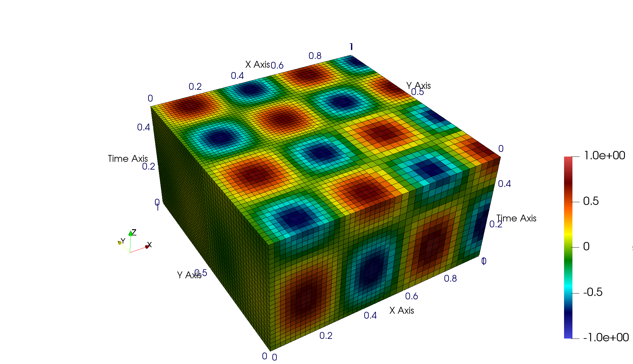
(a) On the whole space-time domain $\Omega^{T}$

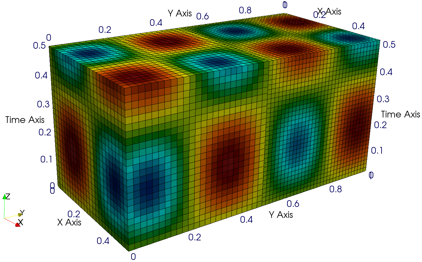
(b) On $\Omega_{1}^{T}\cup\Omega_{4}^{T}$

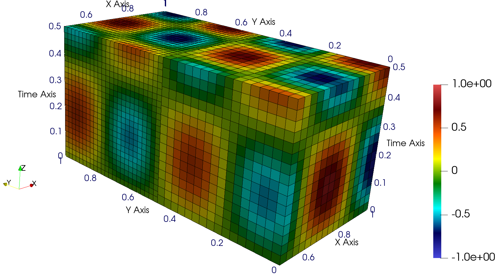
(c) On $\Omega_{2}^{T}\cup\Omega_{3}^{T}$

Figure 2: Example 1, pressure computed using bilinear mortars shown on the space-time grid at refinement 3.

(a) On $\Omega_{1}^{T}\cup\Omega_{4}^{T}$

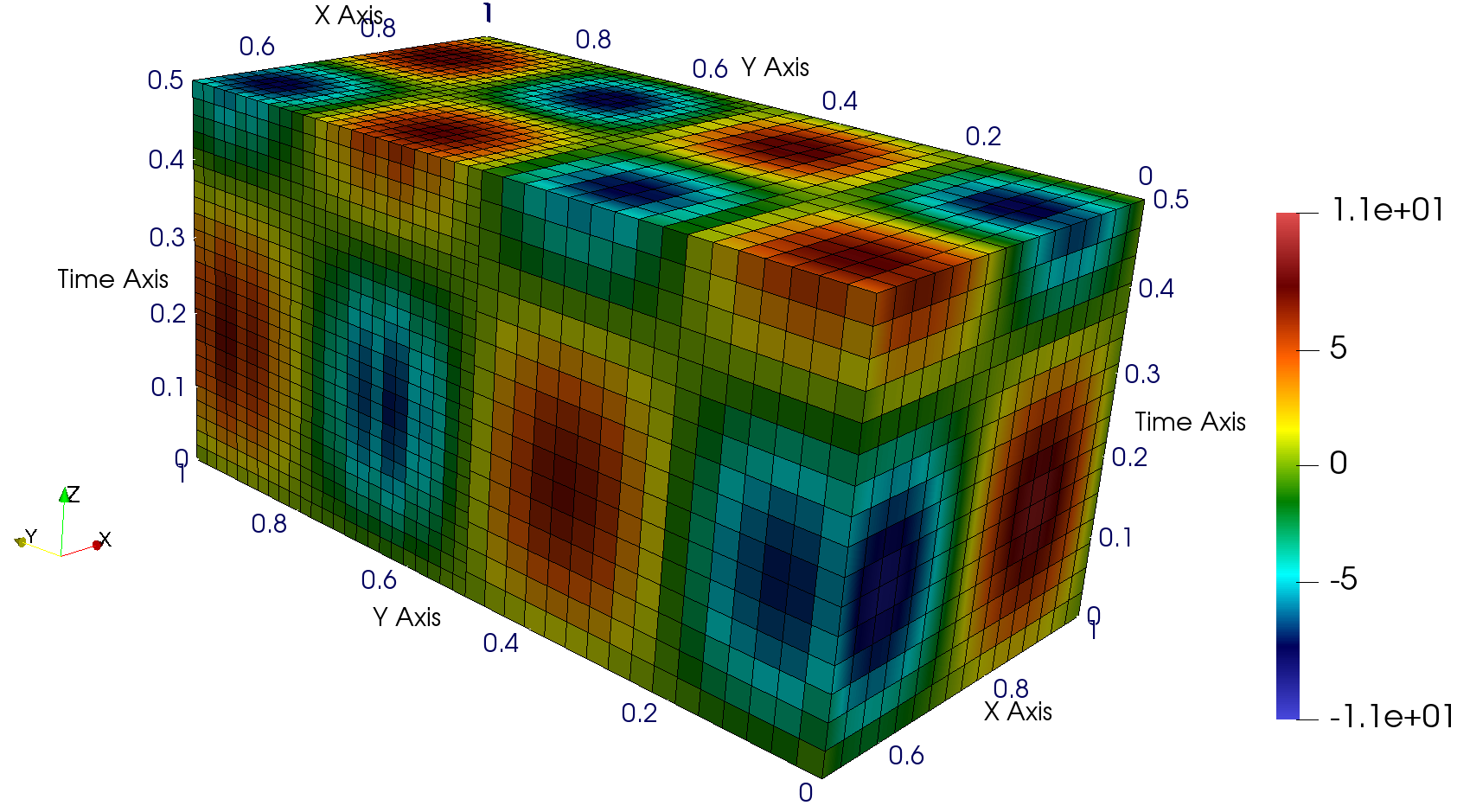
(b) On $\Omega_{2}^{T}\cup\Omega_{3}^{T}$

Figure 3: Example 1, $x$-component of velocity computed using bilinear mortars shown on the space-time grid at refinement 3.

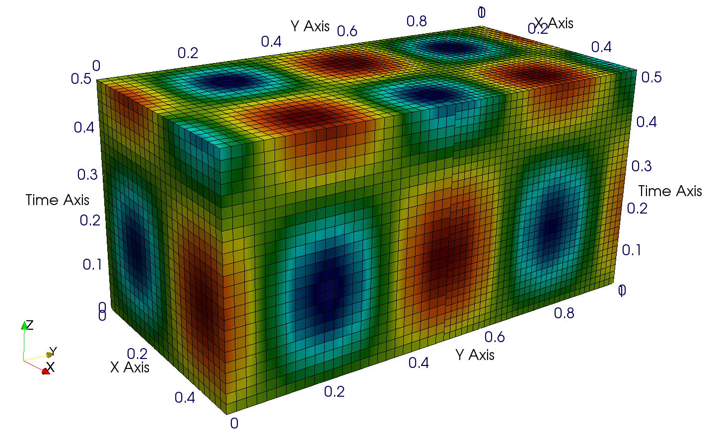
(a) On $\Omega_{1}^{T}\cup\Omega_{4}^{T}$

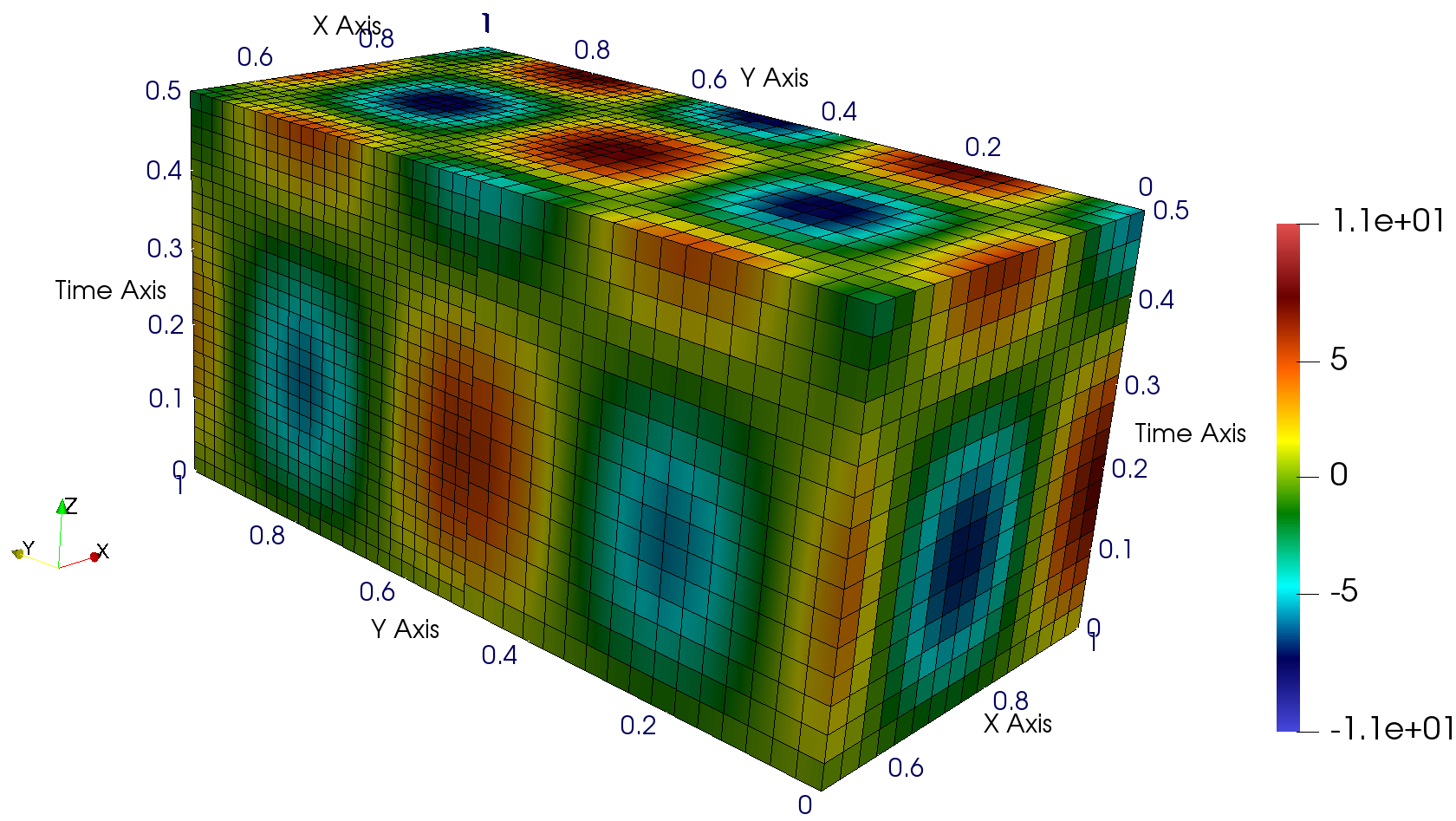
(b) On $\Omega_{2}^{T}\cup\Omega_{3}^{T}$

Figure 4: Example 1, $y$-component of velocity computed using bilinear mortars shown on the space-time grid at refinement 3.

We partition the space domain $\Omega$ into four identical squares $\Omega_{i}$, $i=1,2,3,4$, with $\Omega_{1}=(0,0.5)\times(0,0.5)$, $\Omega_{2}=(0.5,1)\times(0,0.5)$, $\Omega_{3}=(0,0.5)\times(0.5,1)$, and $\Omega_{4}=(0.5,1)\times(0.5,1)$. The space-time domain $\Omega^{T}$ is correspondingly partitioned into four space-time subdomains $\Omega_{i}^{T}$, $i=1,2,3,4$. We start with an initial grid for each $\Omega_{i}^{T}$ and $\Gamma_{ij}^{T}$ and refine it successively 4 times to test the convergence rate of the solutions with respect to the actual known solution. The subdomains $\Omega_{i}^{T}$ maintain a checkerboard non-matching mesh structure throughout the refinement cycles. In particular, let $n_{i}$ be number of elements in either the $x$ or $y$-directions and let $N_{i}$ be the number of elements in the $t$-direction in subdomain $\Omega_{i}^{T}$. The initial grids are chosen as $n_{1}=N_{1}=3$, $n_{2}=N_{2}=2$, $n_{3}=N_{3}=4$, and $n_{4}=N_{4}=3$, see Table 1. Note that $h={\Delta t}$. In the case of bilinear mortars, we maintain $H=2h$ and $\Delta T=2{\Delta t}$, halving the mesh sizes on each refinement cycle. For biquadratic mortars, we start with $H=2h$ and $\Delta T=2{\Delta t}$, but refine the mortar mesh only every other time to maintain $H=\sqrt{h}$ and $\Delta T=\sqrt{{\Delta t}}$. The coarser mesh on $\Gamma^{T}$ in the biquadratic mortar case $DGQ_{2}$ is compensated by the higher degree of the space. In particular, the last term on the right hand side in the bound (5.4) from Theorem 5.1 gives ${\cal O}(h^{-\frac{1}{2}}H^{m+1})$. With $m=1$ and $H={\cal O}(h)$, this results in ${\cal O}(h^{\frac{3}{2}})$, while with $m=2$ and $H={\cal O}(h^{\frac{1}{2}})$, it gives ${\cal O}(h)$. Similarly, the last term in the bound (6.16) from Theorem 6.3 gives ${\cal O}(H^{m+\frac{1}{2}})$. With $m=1$ and $H={\cal O}(h)$, this results in ${\cal O}(h^{\frac{3}{2}})$, while with $m=2$ and $H={\cal O}(h^{\frac{1}{2}})$, it gives ${\cal O}(h^{\frac{5}{4}})$. In all cases, the order is no smaller than the optimal order ${\cal O}(h)$ with respect to the $RT_{0}\times DGQ_{0}$ finite element spaces. More details on the mesh refinement are given in Table 1. There we also report the number of spatial degrees of freedom of the spaces $RT_{0}\times DGQ_{0}$ on $\Omega_{i}$, as well as the number of space-time degrees of freedom of the mortar space $DGQ_{1}$ or $DGQ_{2}$ on $\Gamma^{T}$.

In Tables 2 and 3 we report the relative errors with respect to the norm of the true solution, as well as the convergence rates as powers of the subdomain discretization parameters $h$ and ${\Delta t}$. We observe optimal first order convergence of the method using both bilinear and biquadratic mortars. We note that the ${\Delta t}^{-\frac{1}{2}}$ loss in convergence rate in the bound from Theorem 5.1 is not observed in the numerical results. In Tables 2 and 3 we also report the growth rate for the number of GMRES iterations in the case of bilinear and biquadratic mortars, respectively. We recall that Theorem 7.2 bounds the spectral ratio of the interface operator $S$ by $\mathcal{O}(h^{-1})$. Thus, up to deviation from a normal matrix, the growth rate is expected to be $\mathcal{O}(h^{-0.5})$ [38, 37]. This is close to what we observe in Tables 2 and 3.

We further compare the performance of bilinear and biquadratic mortars. As expected, the accuracy of the two cases at the same refinement level is comparable, which is evident from Tables 2 and 3. On the other hand, since the biquadratic mortar space $DGQ_{2}$ has far fewer degrees of freedom compared to bilinear mortar space $DGQ_{1}$, the former results in a smaller number of GMRES iterations. Thus, choosing higher mortar degrees $m,s$ with a coarser mortar mesh results in a computationally more efficient method compared to using smaller $m,s$ and a finer mortar mesh.

Finally, the computed solution is presented in three-dimensional space-time plots in Figures 2–4. Note that the $z$-axis corresponds to time direction $t$. The plots clearly show the continuity of pressure and velocity, which is imposed in a weak sense, across the space-time interfaces.

8.2 Example 2: problem with a boundary layer

In this example, we demonstrate the advantages of applying the multiscale mortar space-time domain decomposition method to a problem where the solution variables, pressure and velocity, vary on different scales across the space-time domain. For this, we use the known solution, $p(x,y,t)=1000xyt\,e^{-10\left(x^{2}+y^{2}+\frac{1}{4}t^{2}\right)}$ along with permeability $K=I_{2\times 2}$ to determine the right-hand side $q$ in (2.1) and impose Dirichlet boundary condition and initial condition on the space-time domain $\Omega^{T}=(0,1)^{2}\times(0,0.5)$. By construction, $p(x,y,t)$ varies rapidly in both space and time along the lower-left corner of $\Omega^{T}$, forming a sharp boundary layer. The pressure decays exponentially away from this corner and is close to zero over a large part of the domain. This calls for an efficient multiscale method that would take advantage of the multiscale nature of the problem and provide better resolution around the lower-left corner compared to the rest of $\Omega^{T}$.

We partition $\Omega^{T}$ into $4\times 4$ identical space-time subdomains $\Omega^{T}_{i}$. From the knowledge about the variation of the true pressure, we design a multiscale space-time grid on $\Omega^{T}$, where the refinement of the grid on each $\Omega^{T}_{i}$ is proportional to the amount of pressure variation. The finest mesh on $\Omega^{T}_{i}$ has $h=1/128$ and ${\Delta t}=1/64$, and the coarsest mesh on $\Omega^{T}_{i}$ has $h=1/8$ and ${\Delta t}=1/8$, see Figures 5–6 for the mesh refinement. The coarser meshes on the majority of the space-time subdomains reduce the computational complexity of the subdomain solves associated with them. We use a linear mortar ($m=s=1$) on the subdomain interfaces. The mortar mesh sizes in space are chosen as follows. For vertical interfaces (fixed $x$) between subdomains on the bottom row, the one along the boundary layer, we set $H=1/32$. For the next row of subdomains we set $H=1/16$, and for the other two rows, $H=1/8$. Similarly, for the horizontal interfaces (fixed $y$) between subdomains on the left column we set $H=1/32$, for the second column, $H=1/16$, and for the other two columns, $H=1/8$. We choose $\Delta T=1/8$ on all interfaces. These choices guarantee that the mortar assumption (4.6) is satisfied and that the dimension of the interface problem is reduced, while at the same time provide suitable resolution to enforce weakly flux continuity across the space-time interfaces. For comparison, we solve the problem using a uniformly fine and matching subdomain mesh with $h=H=1/128$ and ${\Delta t}={\Delta T}=1/64$. A comparison of the number of GMRES iterations and the relative errors from the multiscale and the fine-scale methods is given in Table 4. It shows that the multiscale and the fine-scale solutions attain comparable accuracy. We observe slightly smaller relative errors in the fine-scale case because of the matching grids and higher resolution throughout the space-time domain. The slightly higher errors for the multiscale method are compensated by the cheaper subdomain solves and smaller interface problem that converges in fewer iterations compared to the fine-scale method.

Table 4: Example 2, errors and GMRES iterations for the multiscale and fine-scale methods

Method	# GMRES	$\|{\bf u}-{\bf u}_{h}^{{\Delta t}}\|_{L^{2}(0,T;{\bf L}^{2}(\Omega))}$	$\|p-p_{h}^{{\Delta t}}\|_{{\rm DG}}$	$\|p-p_{h}^{{\Delta t}}\|_{L^{2}(0,T;W)}$	$\|\lambda-\lambda_{H}^{\Delta T}\|_{L^{2}(0,T;\Lambda_{H})}$
multiscale	102	5.657e-02	8.425e-02	6.319e-02	5.796e-02
fine-scale	140	1.524e-02	2.234e-02	2.154e-02	3.016e-02

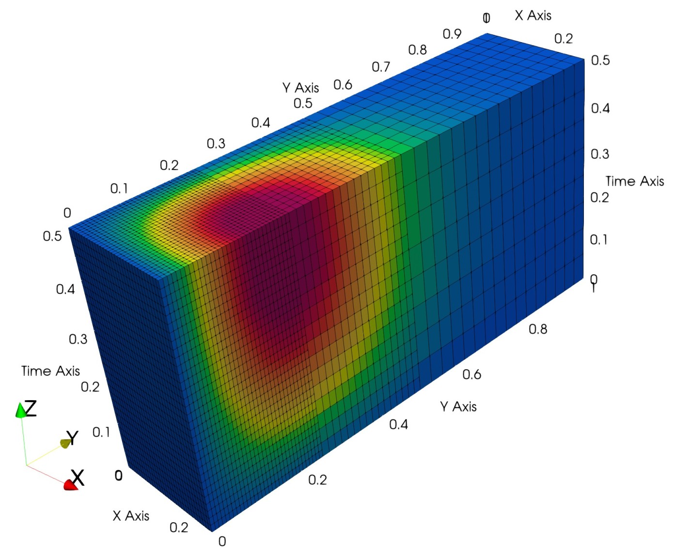
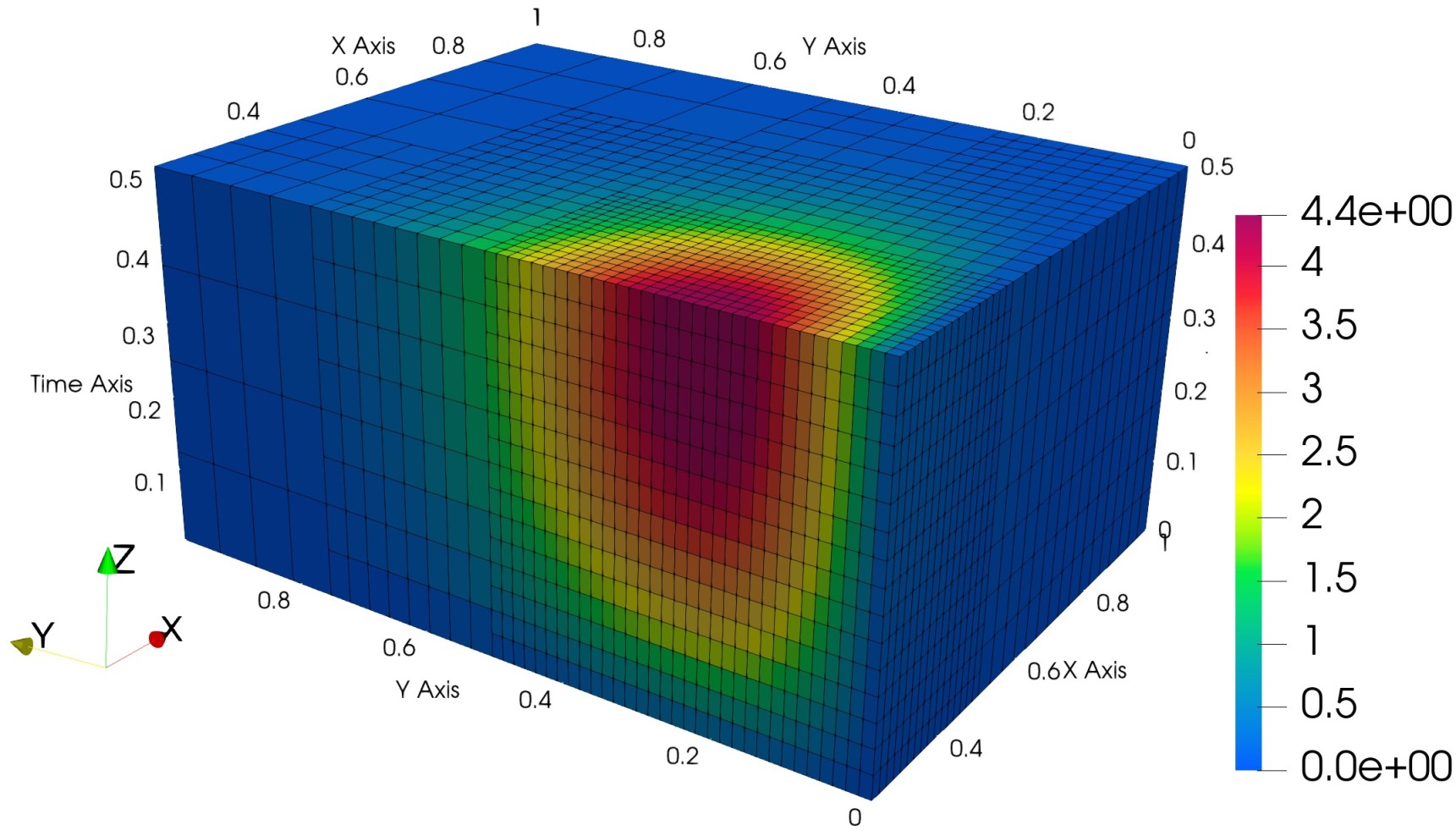
Figure 5: Example 2, pressure from the multiscale method, cut along the plane $x=0.25$.

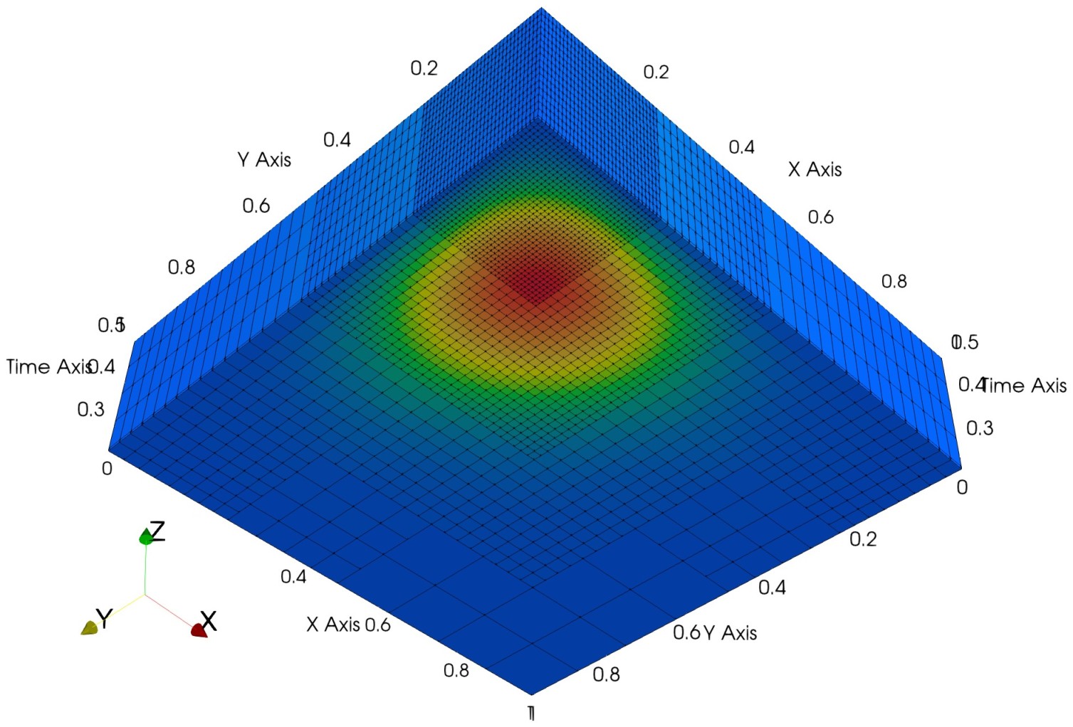
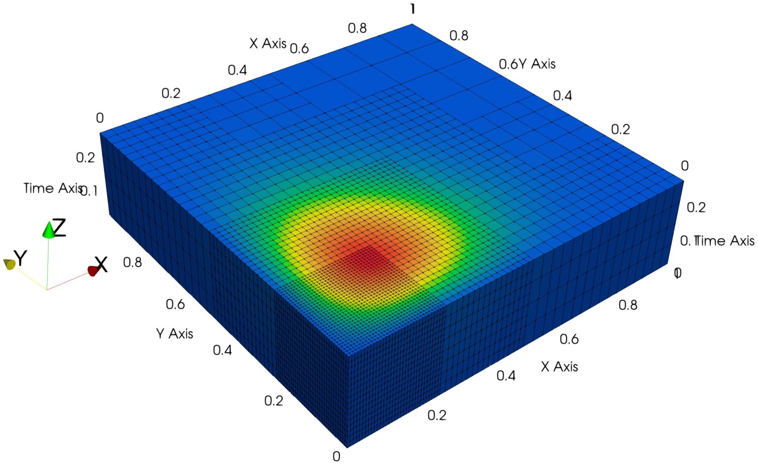
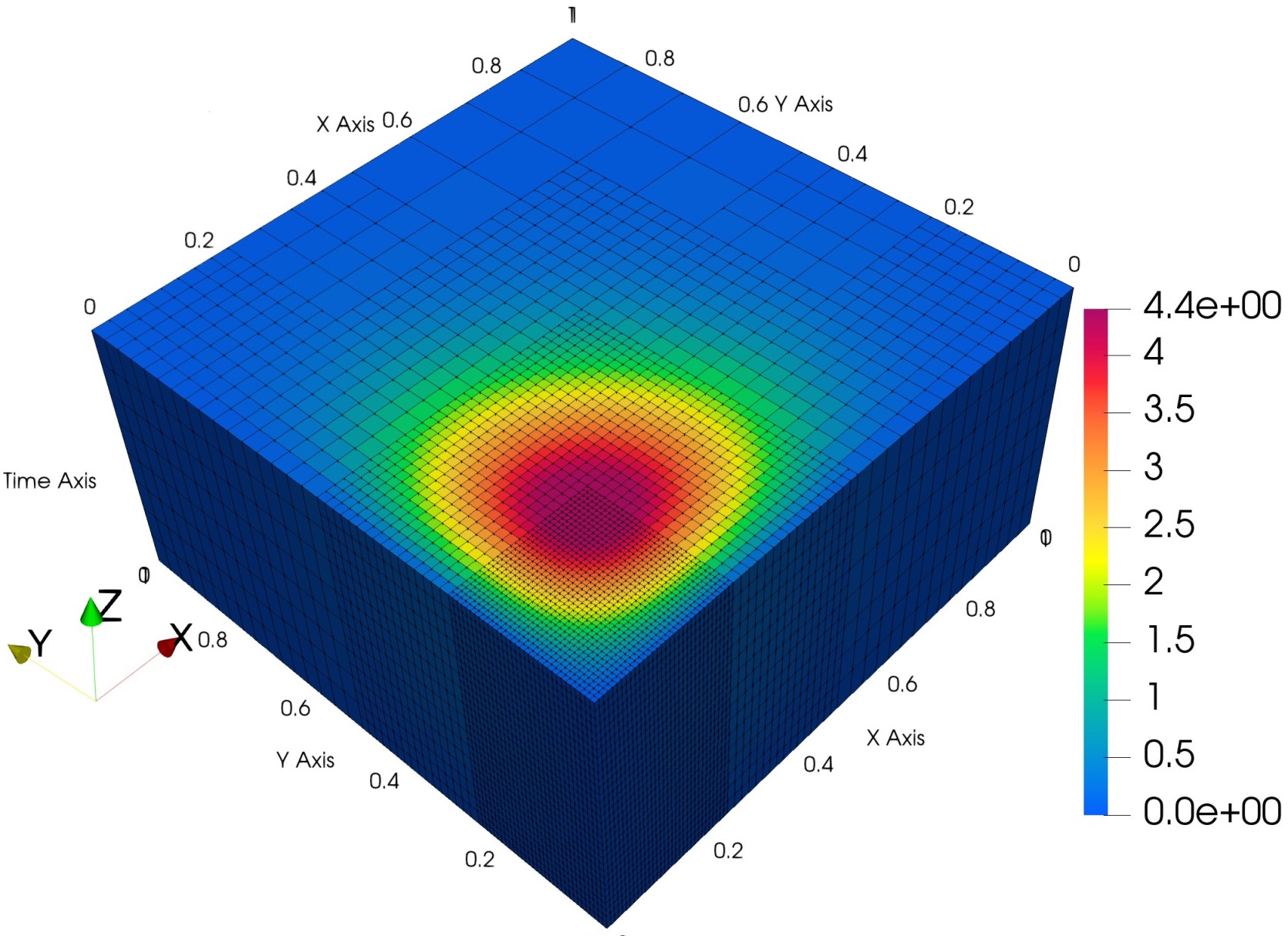
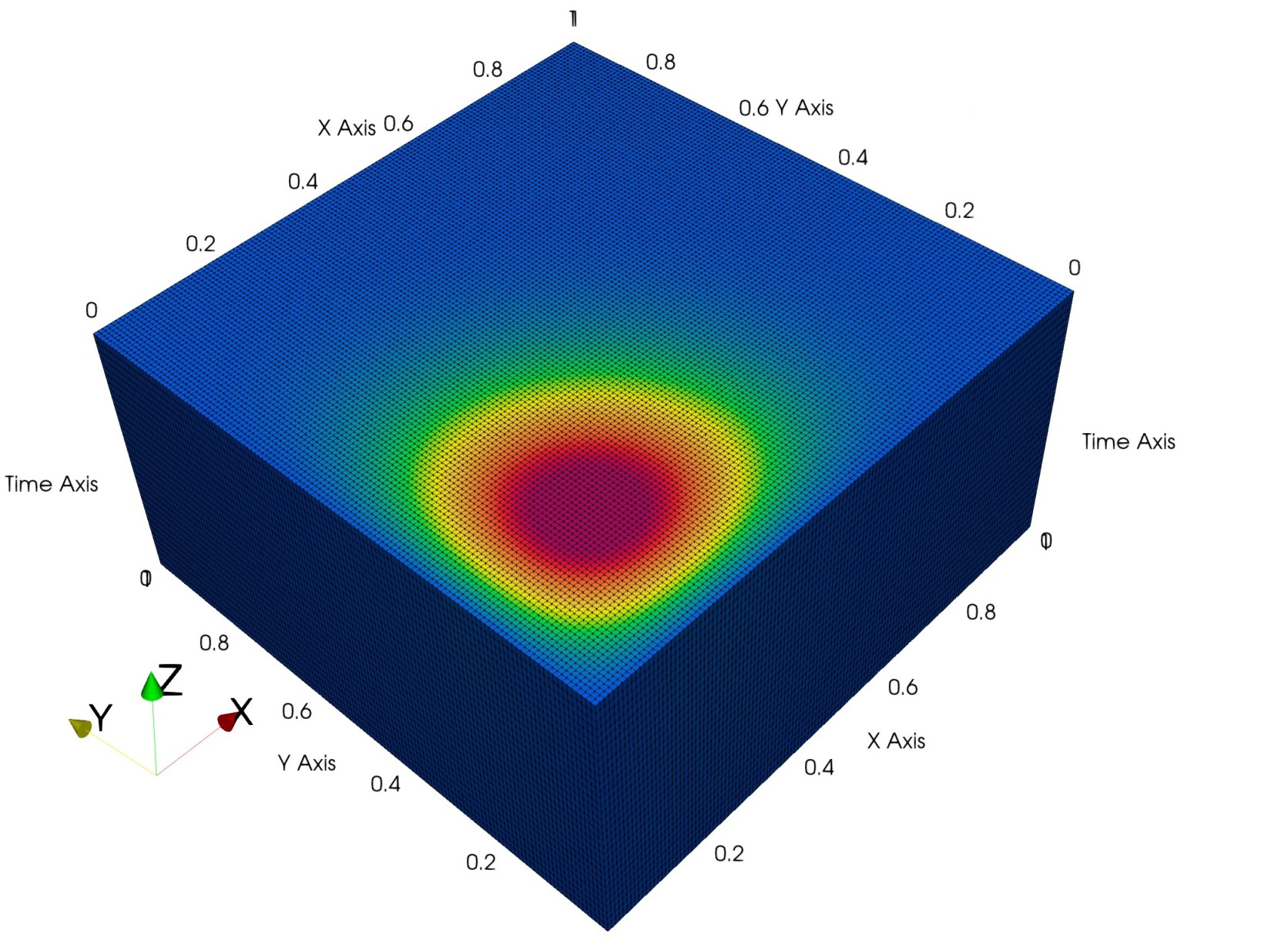
Figure 6: Example 2, left: pressure from the multiscale method, cut along the plane $t=0.35$; right: pressure from the multiscale (top) and fine-scale (bottom) methods on the whole domain.

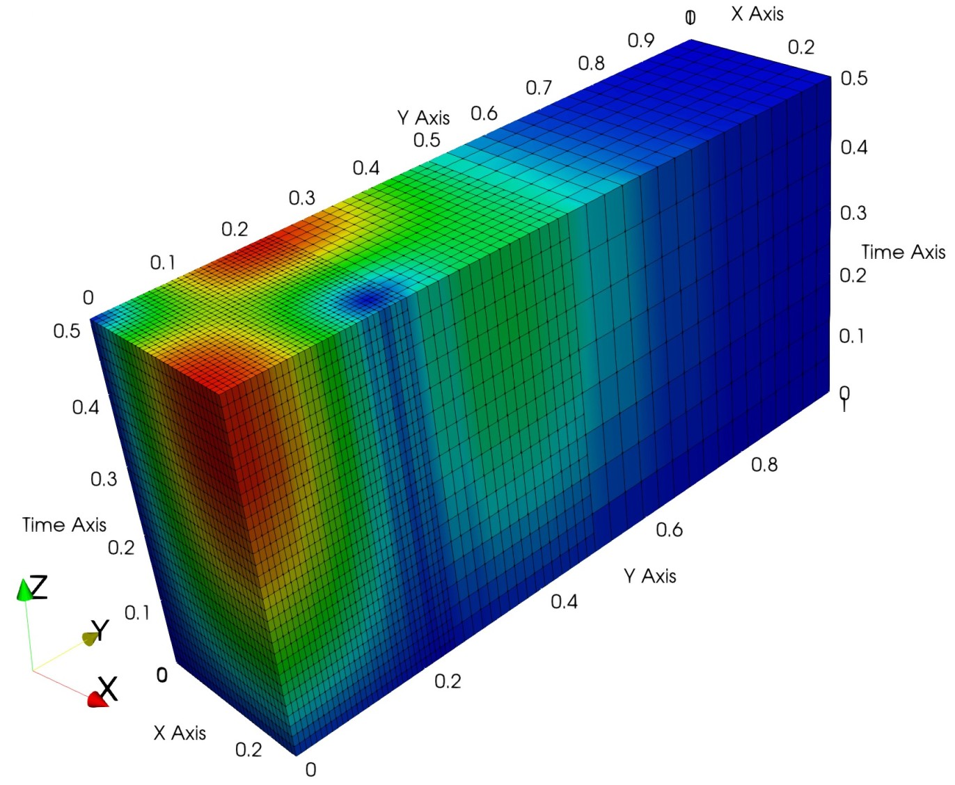
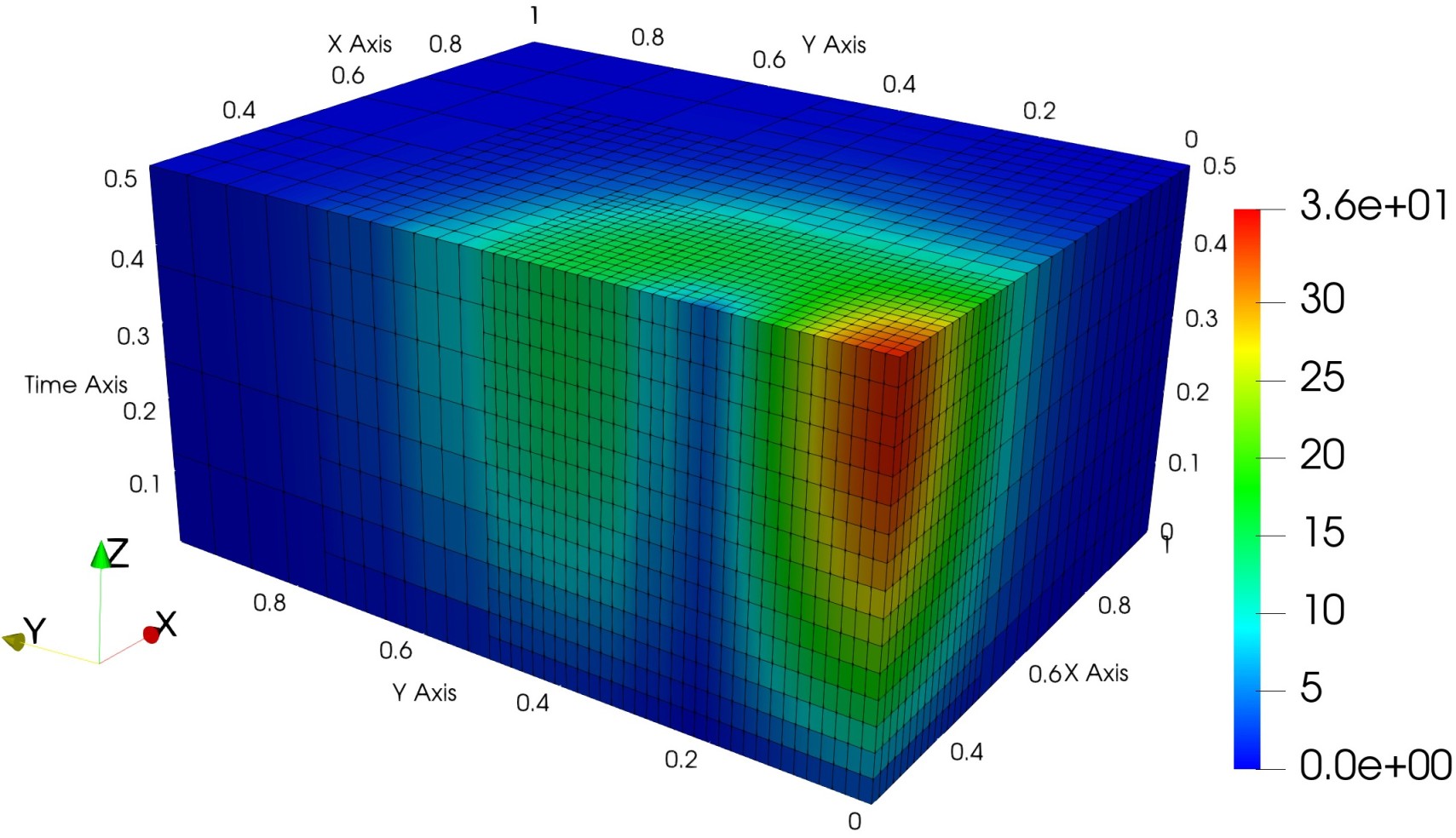
Figure 7: Example 2, velocity magnitude from the multiscale method, cut along the plane $x=0.25$.

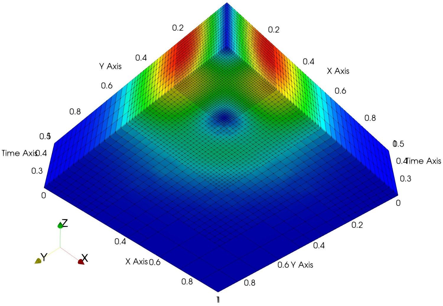
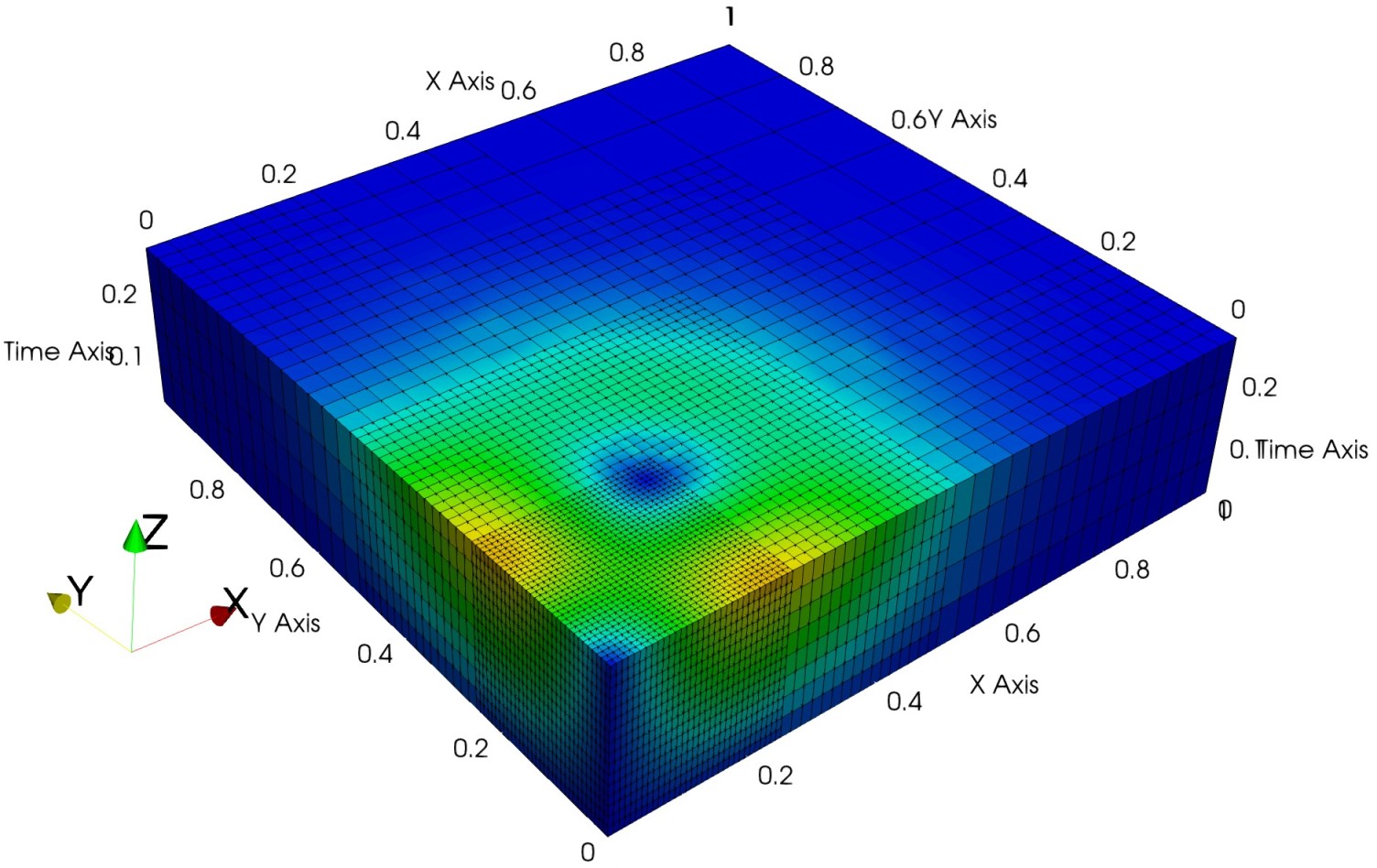
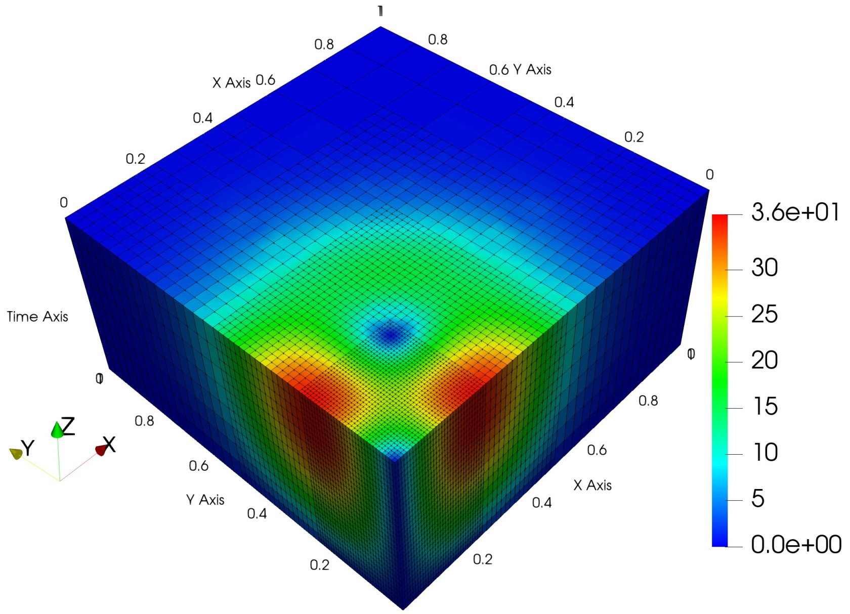
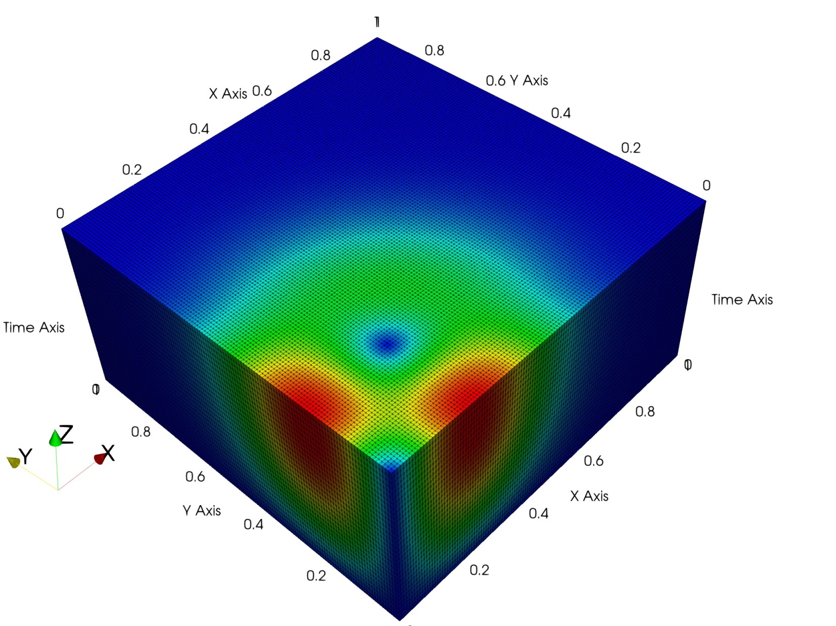
Figure 8: Example 2, left: velocity magnitude from the multiscale method, cut along the plane $t=0.35$; right: velocity magnitude from the multiscale (top) and fine-scale (bottom) methods on the whole domain.

The computed multiscale solution is presented in Figures 5–8. The plots show that the multiscale method provides good resolution where it matters – in the regions with high solution variation. Moreover, we observe very good enforcement of continuity of both pressure and velocity across various space and time interfaces. Side-to-side comparisons of the multiscale and fine-scale solutions are given on the right sides in Figure 6 and Figure 8. They show excellent agreement between the two solutions and once again confirm that the less expensive multiscale method provides comparable accuracy to the more expensive fine-scale method.

9 Conclusions

We presented a space-time domain decomposition mixed finite element method for parabolic problems that allows for non-matching spatial grids and local time stepping via space-time mortar finite elements. Well-posedness and a priori error estimates were established. A parallel non-overlapping domain decomposition algorithm was developed, which reduces the algebraic problem to a coarse-scale interface problem for the mortar variable. The theoretical results and the flexibility of the method were illustrated in a series of numerical experiments. Future work may include the development and analysis of a Neumann–Neumann preconditioner for the interface problem in Section 7 as in [33], using techniques from [46], as well as deriving a posteriori error estimates, possibly building upon the ideas from [18, 1, 2].

References

- [1] S. Ali Hassan, C. Japhet, M. Kern, and M. Vohralík. A posteriori stopping criteria for optimized Schwarz domain decomposition algorithms in mixed formulations. Comput. Methods Appl. Math., 18(3):495–519, 2018.
- [2] S. Ali Hassan, C. Japhet, and M. Vohralík. A posteriori stopping criteria for space-time domain decomposition for the heat equation in mixed formulations. Electron. Trans. Numer. Anal., 49:151–181, 2018.
- [3] T. Arbogast, L. C. Cowsar, M. F. Wheeler, and I. Yotov. Mixed finite element methods on nonmatching multiblock grids. SIAM J. Numer. Anal., 37(4):1295–1315, 2000.
- [4] T. Arbogast, D. Estep, B. Sheehan, and S. Tavener. A posteriori error estimates for mixed finite element and finite volume methods for parabolic problems coupled through a boundary. SIAM/ASA J. Uncertain. Quantif., 3(1):169–198, 2015.
- [5] T. Arbogast, G. Pencheva, M. F. Wheeler, and I. Yotov. A multiscale mortar mixed finite element method. Multiscale Model. Simul., 6(1):319–346, 2007.
- [6] M. Arshad, E.-J. Park, and D. Shin. Multiscale mortar mixed domain decomposition approximations of nonlinear parabolic equations. Comput. Math. Appl., 97:375–385, 2021.
- [7] W. Bangerth, R. Hartmann, and G. Kanschat. deal.II—a general-purpose object-oriented finite element library. ACM Trans. Math. Software, 33(4):Art. 24, 27, 2007.
- [8] M. Bause, F. A. Radu, and U. Köcher. Error analysis for discretizations of parabolic problems using continuous finite elements in time and mixed finite elements in space. Numer. Math., 137(4):773–818, 2017.
- [9] B. Beckermann, S. A. Goreinov, and E. E. Tyrtyshnikov. Some remarks on the Elman estimate for GMRES. SIAM J. Matrix Anal. Appl., 27(3):772–778, 2005.
- [10] M. Beneš, A. Nekvinda, and M. K. Yadav. Multi-time-step domain decomposition method with non-matching grids for parabolic problems. Appl. Math. Comput., 267:571–582, 2015.
- [11] F. Brezzi and M. Fortin. Mixed and hybrid finite element methods. Springer-Verlag, New York, 1991.
- [12] J. M. Cascón, L. Ferragut, and M. I. Asensio. Space-time adaptive algorithm for the mixed parabolic problem. Numer. Math., 103(3):367–392, 2006.
- [13] P. G. Ciarlet. The finite element method for elliptic problems. North-Holland Publishing Co., Amsterdam-New York-Oxford, 1978. Studies in Mathematics and its Applications, Vol. 4.
- [14] M. Crouzeix and V. Thomée. The stability in and of the -projection onto finite element function spaces. Math. Comp., 48(178):521–532, 1987.
- [15] C. N. Dawson, Q. Du, and T. F. Dupont. A finite difference domain decomposition algorithm for numerical solution of the heat equation. Math. Comp., 57(195):63–71, 1991.
- [16] L. Delpopolo Carciopolo, M. Cusini, L. Formaggia, and H. Hajibeygi. Adaptive multilevel space-time-stepping scheme for transport in heterogeneous porous media (ADM-LTS). J. Comput. Phys. X, 6:100052, 21, 2020.
- [17] S. C. Eisenstat, H. C. Elman, and M. H. Schultz. Variational iterative methods for nonsymmetric systems of linear equations. SIAM J. Numer. Anal., 20(2):345–357, 1983.
- [18] A. Ern, I. Smears, and M. Vohralík. Guaranteed, locally space-time efficient, and polynomial-degree robust a posteriori error estimates for high-order discretizations of parabolic problems. SIAM J. Numer. Anal., 55(6):2811–2834, 2017.
- [19] R. E. Ewing, R. D. Lazarov, and P. S. Vassilevski. Finite difference schemes on grids with local refinement in time and space for parabolic problems. I. Derivation, stability, and error analysis. Computing, 45(3):193–215, 1990.
- [20] R. D. Falgout, S. Friedhoff, T. V. Kolev, S. P. MacLachlan, and J. B. Schroder. Parallel time integration with multigrid. SIAM J. Sci. Comput., 36(6):C635–C661, 2014.
- [21] V. Faucher and A. Combescure. A time and space mortar method for coupling linear modal subdomains and non-linear subdomains in explicit structural dynamics. Comput. Methods Appl. Mech. Engrg., 192(5):509–533, 2003.
- [22] S. Gaiffe, R. Glowinski, and R. Masson. Domain decomposition and splitting methods for mortar mixed finite element approximations to parabolic equations. Numer. Math., 93(1):53–75, 2002.
- [23] M. J. Gander. 50 years of time parallel time integration. In Multiple shooting and time domain decomposition methods. MuS-TDD, Heidelberg, Germany, May 6–8, 2013, pages 69–113. Cham: Springer, 2015.
- [24] M. J. Gander and L. Halpern. Optimized Schwarz waveform relaxation methods for advection reaction diffusion problems. SIAM J. Numer. Anal., 45(2):666–697, 2007.
- [25] M. J. Gander, F. Kwok, and B. C. Mandal. Dirichlet-Neumann and Neumann-Neumann waveform relaxation algorithms for parabolic problems. Electron. Trans. Numer. Anal., 45:424–456, 2016.
- [26] M. J. Gander and M. Neumüller. Analysis of a new space-time parallel multigrid algorithm for parabolic problems. SIAM J. Sci. Comput., 38(4):A2173–A2208, 2016.
- [27] M. J. Gander and S. Vandewalle. Analysis of the parareal time-parallel time-integration method. SIAM J. Sci. Comput., 29(2):556–578, 2007.
- [28] B. Ganis and I. Yotov. Implementation of a mortar mixed finite element method using a multiscale flux basis. Comput. Methods Appl. Mech. Engrg., 198(49):3989–3998, 2009.
- [29] A. Greenbaum. Iterative methods for solving linear systems, volume 17 of Frontiers in Applied Mathematics. Society for Industrial and Applied Mathematics (SIAM), Philadelphia, PA, 1997.
- [30] P. Grisvard. Elliptic problems in nonsmooth domains, volume 69 of Classics in Applied Mathematics. Society for Industrial and Applied Mathematics (SIAM), Philadelphia, PA, 2011.
- [31] C. Hager, P. Hauret, P. Le Tallec, and B. I. Wohlmuth. Solving dynamic contact problems with local refinement in space and time. Comput. Methods Appl. Mech. Engrg., 201/204:25–41, 2012.
- [32] L. Halpern, C. Japhet, and J. Szeftel. Optimized Schwarz waveform relaxation and discontinuous Galerkin time stepping for heterogeneous problems. SIAM J. Numer. Anal., 50(5):2588–2611, 2012.
- [33] T.-T.-P. Hoang, J. Jaffré, C. Japhet, M. Kern, and J. E. Roberts. Space-time domain decomposition methods for diffusion problems in mixed formulations. SIAM J. Numer. Anal., 51(6):3532–3559, 2013.
- [34] T.-T.-P. Hoang, C. Japhet, M. Kern, and J. E. Roberts. Space-time domain decomposition for reduced fracture models in mixed formulation. SIAM J. Numer. Anal., 54(1):288–316, 2016.
- [35] T.-T.-P. Hoang and H. Lee. A global-in-time domain decomposition method for the coupled nonlinear Stokes and Darcy flows. J. Sci. Comp., 87(1):1–22, 2021.
- [36] R. A. Horn and C. R. Johnson. Topics in matrix analysis. Cambridge University Press, Cambridge, 1994. Corrected reprint of the 1991 original.
- [37] I. C. F. Ipsen. Expressions and bounds for the GMRES residual. BIT, 40(3):524–535, 2000.
- [38] C. T. Kelley. Iterative methods for linear and nonlinear equations, volume 16 of Frontiers in Applied Mathematics. Society for Industrial and Applied Mathematics, Philadelphia, 1995.
- [39] W. Kheriji, R. Masson, and A. Moncorgé. Nearwell local space and time refinement in reservoir simulation. Math. Comput. Simulation, 118:273–292, 2015.
- [40] D. Kim, E.-J. Park, and B. Seo. Space-time adaptive methods for the mixed formulation of a linear parabolic Problem. J. Sci. Comput., 74(3):1725–1756, 2018.
- [41] D. Krause and R. Krause. Enabling local time stepping in the parallel implicit solution of reaction-diffusion equations via space-time finite elements on shallow tree meshes. Appl. Math. Comput., 277:164–179, 2016.
- [42] J.-L. Lions, Y. Maday, and G. Turinici. Résolution d’EDP par un schéma en temps “pararéel”. C. R. Acad. Sci., Paris, Sér. I, Math., 332(7):661–668, 2001.
- [43] J.-L. Lions and E. Magenes. Non-homogeneous boundary value problems and applications. Vol. I. Springer-Verlag, New York-Heidelberg, 1972.
- [44] C. Makridakis and R. H. Nochetto. A posteriori error analysis for higher order dissipative methods for evolution problems. Numer. Math., 104:489–514, 2006.
- [45] P. B. Nakshatrala, K. B. Nakshatrala, and D. A. Tortorelli. A time-staggered partitioned coupling algorithm for transient heat conduction. Internat. J. Numer. Methods Engrg., 78(12):1387–1406, 2009.
- [46] G. Pencheva and I. Yotov. Balancing domain decomposition for mortar mixed finite element methods. Numer. Linear Algebra Appl., 10(1-2):159–180, 2003.
- [47] I. Rybak and J. Magiera. A multiple-time-step technique for coupled free flow and porous medium systems. J. Comput. Phys., 272:327–342, 2014.
- [48] L. R. Scott and S. Zhang. Finite element interpolation of nonsmooth functions satisfying boundary conditions. Math. Comput., 54(190):483–493, 1990.
- [49] G. Starke. Field-of-values analysis of preconditioned iterative methods for nonsymmetric elliptic problems. Numer. Math., 78(1):103–117, 1997.
- [50] V. Thomée. Galerkin finite element methods for parabolic problems, volume 25 of Springer Series in Computational Mathematics. Springer-Verlag, Berlin, second edition, 2006.
- [51] H. Yu. A local space-time adaptive scheme in solving two-dimensional parabolic problems based on domain decomposition methods. SIAM J. Sci. Comput., 23(1):304–322, 2001.