Thermometry of Gaussian quantum systems using Gaussian measurements
Abstract
We study the problem of estimating the temperature of Gaussian systems with feasible measurements, namely Gaussian and photo-detection-like measurements. For Gaussian measurements, we develop a general method to identify the optimal measurement numerically, and derive the analytical solutions in some relevant cases. For a class of single-mode states that includes thermal ones, the optimal Gaussian measurement is either Heterodyne or Homodyne, depending on the temperature regime. This is in contrast to the general setting, in which a projective measurement in the eigenbasis of the Hamiltonian is optimal regardless of temperature. In the general multi-mode case, and unlike the general unrestricted scenario where joint measurements are not helpful for thermometry (nor for any parameter estimation task), it is open whether joint Gaussian measurements provide an advantage over local ones. We conjecture that they are not useful for thermal systems, supported by partial analytical and numerical evidence. We further show that Gaussian measurements become optimal in the limit of large temperatures, while on/off photo-detection-like measurements do it for when the temperature tends to zero. Our results therefore pave the way for effective thermometry of Gaussian quantum systems using experimentally realizable measurements.
1 Introduction and motivation
The high precision required for the operation of quantum devices demands for the estimation of their parameters with minimum possible error. In particular, estimating temperature is a problem that has attained substantial popularity in recent years [Mehboudi et al.(2019a)Mehboudi, Sanpera, and Correa, De Pasquale and Stace(2018)], since it is a parameter that highly impacts the technological usage of quantum systems. Thermometry process, like any other parameter estimation problem, can be seen as different stages of (i) preparation of a probe or thermometer, (ii) interaction of the probe with the sample, and (iii) measurement of the probe and data analysis [Giovannetti et al.(2011)Giovannetti, Lloyd, and Maccone, Giovannetti et al.(2006)Giovannetti, Lloyd, and Maccone, Tóth and Apellaniz(2014)], see also Fig. 1. When there are no restrictions on any of these stages, one finds the ultimate limits on thermometry precision [Mehboudi et al.(2019a)Mehboudi, Sanpera, and Correa, De Pasquale and Stace(2018)]. These limits have deeply increased our understanding of fundamental restrictions/possibilities in any thermometry procedure [Correa et al.(2015)Correa, Mehboudi, Adesso, and Sanpera]. Nonetheless, one also needs to address frameworks that are experimentally feasible, hence revisit the fundamental limits subject to experimental restrictions on the different stages above. In this work, we are in particular concerned with restrictions on the performed measurements, stage (iii) above. To our knowledge, there have been so far few works addressing measurement restrictions, such as limited resolution [Jorgensen et al.(2020)Jorgensen, Potts, Paris, and Brask] or coarse grained measurements [Hovhannisyan et al.(2021)Hovhannisyan, J0rgensen, Landi, Alhambra, Brask, and Perarnau-Llobet], in thermometry applications.
Our main goal is to study the use of experimentally feasible measurements in thermometry processes using continuous variable (CV) Gaussian systems. CV Gaussian models are very successful at describing various physical systems of relevance, such as Bosonic gases, electromagnetic fields, mechanical oscillators and Josephson junctions, to name a few. This makes them versatile candidates for several quantum information processing as well as quantum simulation tasks [Weedbrook et al.(2012)Weedbrook, Pirandola, García-Patrón, Cerf, Ralph, Shapiro, and Lloyd, Lewenstein et al.(2007)Lewenstein, Sanpera, Ahufinger, Damski, Sen(De), and Sen, Lewenstein et al.(2012)Lewenstein, Sanpera, and Ahufinger, Serafini(2017), Diamanti and Leverrier(2015), Navascués and Acín(2005)]. When there is no limitation on the performed measurements, thermometry (and more generally metrology) of Gaussian CV systems is characterized readily, in particular the optimal measurement and the ultimate precision can be found analytically [Monras(2013), Jiang(2014), Nichols et al.(2018)Nichols, Liuzzo-Scorpo, Knott, and Adesso]. Nonetheless, a rigorous analysis of quantum metrology with realistic measurements, namely Gaussian as well as two-outcome photo-detection measurements, is missing. Our work addresses this question in the context of temperature estimation.
Several previous theoretical works have already focused on thermometry via Gaussian probes, e.g., exploiting Bosonic impurities embedded in cold gases, or light modes that interact with an external field [Mehboudi et al.(2019b)Mehboudi, Lampo, Charalambous, Correa, García-March, and Lewenstein, Planella et al.(2022)Planella, Cenni, Acín, and Mehboudi, Correa et al.(2017)Correa, Perarnau-Llobet, Hovhannisyan, Hernández-Santana, Mehboudi, and Sanpera, Hovhannisyan and Correa(2018), Mukherjee et al.(2019)Mukherjee, Zwick, Ghosh, Chen, and Kurizki, Martín-Martínez et al.(2013)Martín-Martínez, Dragan, Mann, and Fuentes]. Unfortunately, in these systems the optimal measurement for thermometry can be experimentally very demanding and effectively out of reach. For example, consider a scenario where a light mode is used as thermometer. After interacting with a sample with an unknown temperature , the light mode can relax to a thermal state with the same temperature. By performing measurements on the light mode one aims to estimate the temperature. The maximally informative measurement in this case is an energy measurement. This corresponds to ideal photon-counting, which is extremely difficult. It is thus advisable to investigate experimentally realisable measurements, such as realistic on/off photo-detection or Gaussian measurements and benchmark their performance by comparing them with the known optimal measurement. In this work, we follow this approach and first consider single-mode systems. We analytically prove that the optimal Gaussian measurement corresponds to a homodyne or heterodyne measurement, depending on the temperature. We investigate the conditions under which the ultimate bound on thermometry precision is attained. The appendix is there for self-containedness…. We find that at high temperatures Gaussian measurements are almost optimal, while they perform poorly in the low-temperature regime, where, in turn, on/off photo-detection is close to optimal. We then move to the multi-mode scenario. While in the case where measurements are not restricted the additivity of the Fisher information implies that the optimal measurement consist of the independent application of the optimal measurement for single modes, whether the same holds true when restricting the measurements to be Gaussian is open. We conjecture—supported by numerical evidence—that this is indeed the case, and analytically prove it for special cases.
2 Preliminaries: The Phase-space formalism
We start by setting up the notation and introducing the necessary tools from the phase-space formalism, such as Gaussian systems and Gaussian measurements. For additional details, we refer the interested reader to the more complete references [Holevo(2011), Barnett and Radmore(2002), Serafini(2017)]. The basics of parameter estimation in Gaussian systems is discussed in the next section, where we also present some of our results.
2.1 Gaussian States and Measurements
Every trace class111A linear bounded operator acting on a separable Hilbert space is said to be of trace class if , where , and for a positive semidefinite the formal trace can be shown not to depend on the chosen orthonormal basis of . operator defined in a Hilbert space has an equivalent representation in terms of -ordered Phase-space Quasi-probability Distributions [()-PQDs], which are distributions defined over a real symplectic space that is referred to as phase-space. In order to characterize this representation, we first define the frame operators. These operators are denoted by and are often used to define the -ordered quasi-probability distributions corresponding to the operator , that can either be an observable or a density operator in the Hilbert space222Throughout this paper we use a notation in which phase space related quantities are in bold font, e.g., and represent the covariance matrix and displacement vector. On the contrary, we write the operators in the Hilbert space of the system in normal font, e.g., represents the density matrix. For the positive operator-valued measure (POVM) elements like the operator itself is in the Hilbert space and represented with normal font, but the outcome is often a phase-space vector like thus we use the bold font..
First we note that, for a given quantum state and any set of POVM operators —with labeling the specific choice of POVM and the different outcomes for that given choice—the outcome probabilities for the measurements are given by the Born rule,
| (1) |
To show how any -mode operator like can be represented by ()-PQDs in phase-space, we start by expanding in terms of the canonical displacement operators,
| (2) |
where is the displacement (or Weyl) operator, is the vector of canonical quadrature operators, , and , and is the symplectic form enforcing the uncertainty relations in phase-space.
The operators are defined as the Fourier transforms of the displacement operator
| (3) |
where the integral is intended to converge in the weak operator topology. The Wigner function for the density operator is then given by
| (4) |
Since , the operator satisfies the following relations:
| (5) |
and
| (6) |
where we have used that
| (7) |
By taking the inverse Fourier transform of Eq. (4) and using Eq. (7), one obtains
| (8) |
Substituting Eq. (8) into Eq. (2) gives
| (9) | ||||
Finally, by using these results in Eq. (1), we obtain
| (10) |
where is the Wigner function associated to the POVM measurement operators.333The only measurement operators we will encounter will be of trace class. From this relation, we see that the information contained in the probabilities given by Eq. (1) is equivalently contained in the integral overlap of the corresponding Wigner functions.
2.1.1 The overlap of two systems
For any two quantum states and we can use (2) to compute their overlap
| (11) |
Now, the term is nothing but the characteristic function of the th system. That is, by definition,
| (12) |
For Gaussian systems with covariance matrices and displacement operators , the characteristic function is given by the Gaussian distribution
| (13) |
with the displacement vector and the covariance matrix (CM) defined as , and , where and represents the anti-commutator. Having this form for the Gaussian characteristic function, we can write
| (14) |
where we define , and . In order to solve this last integral, we need to find the orthogonal basis of , such that the integration variables decouple. Performing this elementary transformation yields
| (15) |
The Gaussian measurement operators of interest here can be written as displaced Gaussian states , with the displacement vector and the covariance matrix given by and , respectively.444When necessary we use the superscript to refer to measurement operators, displacement vectors, and covariance matrices, to prevent confusion with those of the system. We can write
| (16) |
Our aim is then to find the characteristic function of this Gaussian POVM element. By using the cyclic property of the trace, and the properties of the displacement operator , and , we have that
| (17) |
which means that—up to a constant— has a Gaussian characteristic function with the same covariance matrix as , but with displacement vector increased by the amount referring to the measurement outcome. By putting the pieces together, we have that, for a Gaussian measurement performed on a Gaussian state with displacement vector and CM , the outcome probability distribution takes the (also Gaussian) form
| (18) |
where and are respectively the displacement vector and the covariance matrix of , i.e., the Gaussian state of the measurement. The above is the most general form of the probability distribution of the outcome of a Gaussian measurement on a Gaussian state; however, in what follows we shall assume for simplicity that both and have vanishing displacements, so that
| (19) |
The normalisation of this probability can be checked easily
| (20) |
See the appendix for a generalisation of Gaussian measurements that incorporates noise and auxiliary modes.
3 Thermometry of Gaussian quantum systems: Optimal vs feasible measurements
As already advanced, we are interested in the measurement part of thermometry protocols. Let us first recall some basics of metrology in quantum systems. Given a quantum system we aim to estimate a parameter like temperature imprinted on its density matrix denoted by . To this end, one performs a POVM measurement with positive elements , where labels the specific measurement and the different outcomes for that specific measurement. We have for all , with being the identity operator. The outcomes of the measurement are then mapped into an estimate of the true parameter by using an estimator function . One can quantify the error on such an estimation process by means of the mean square error , with being the probability of observing the outcome conditioned on measuring . Notice that the estimation error depends on the performed measurement. It is well known that for any unbiased estimator, that is, for any estimator satisfying , the mean square error is lower bounded by the Cramér-Rao bound
| (21) |
with being the (classical) Fisher information given by
| (22) |
The Cramér-Rao bound can be saturated in the asymptotic limit by choosing the maximum likelihood estimator [Newey and McFadden(1994)]. A good candidate to quantify the precision of measurements is therefore given by the Fisher information; the larger, the more precise the measurement.
It is a natural and fundamental question to ask: what is the ultimate bound on precision? This is obtained by finding the measurement that minimises Eq. (21). The corresponding precision is quantified by the so-called quantum Fisher information (QFI), which can be formally defined as
| (23) |
Here, is the symmetric logarithmic derivative (SLD), a Hermitian operator defined by
| (24) |
The SLD also characterizes the optimal measurement, which turns out to be projective in the basis of .
3.1 Ultimate bounds on thermometry of Gaussian systems
The problem of finding the ultimate bounds in parameter estimation of Gaussian quantum systems was first addressed in [Monras(2013), Pinel et al.(2013)Pinel, Jian, Treps, Fabre, and Braun], further explored in [Jiang(2014)], and extended to multiple parameter estimation in [Nichols et al.(2018)Nichols, Liuzzo-Scorpo, Knott, and Adesso]. It was shown that the optimal measurement can be always written as a second order operator in terms of the quadratures, that is
| (25) |
where is a matrix of real numbers, is a dimensional real vector, and is a real number. These three quantities are given by the solution of the following equations:
| (26) | ||||
| (27) | ||||
| (28) |
In turn, the quantum Fisher information reads
| (29) |
Despite its elegant and simple form, the optimal measurement (25) is, unfortunately, often an experimentally challenging one to perform. Thus, we will explore more feasible measurements in the next sections. It is worth mentioning that the problem of phase estimation by means of Gaussian measurements has been addressed in [Monras(2006), Oh et al.(2019)Oh, Lee, Rockstuhl, Jeong, Kim, Nha, and Lee] for a single mode, while using Gaussian measurements in the Bayesian approach to metrology was considered in [Morelli et al.(2021)Morelli, Usui, Agudelo, and Friis, Kundu et al.(2022)Kundu, McKay, and Mallik].
3.2 Thermometry using Gaussian measurements
Gaussian measurements are an important family of experimentally realisable measurements. They have been defined formally in section 2.1; alternatively, they can be characterized as all those measurements that are realizable by appending ancillas in the vacuum state, applying arbitrary Gaussian unitaries, and performing homodyne detections [Giedke and Ignacio Cirac(2002)]. We can characterize them by means of their covariance matrix . Our first observation is that the optimal measurement should have a covariance matrix representing a pure quantum state.
3.2.1 Observation.—Pure Gaussian measurements are always better
To prove this claim, we show that any non-pure Gaussian measurement can be cast as classical post-processing of another pure Gaussian measurement, therefore, not increasing its (classical Fisher) information.
The POVM elements of a Gaussian measurement can be written in the form
| (30) |
If the measurement is not pure, then there exists a pure covariance matrix s.t. . This follows directly from Williamson’s theorem [Williamson(1936)] (see also [Lami et al.(2017)Lami, Hirche, Adesso, and Winter, Lemma 5] for a direct proof). The POVM measurement elements corresponding to this pure CM are
| (31) |
If can be reproduced by , then we should find the probability measure s.t.,
| (32) |
By combining (31) and (32) we obtain
| (33) |
If we compare with (30), we should have
| (34) |
Finally by taking the inverse Fourier transform we find
| (35) |
Note that the fact that the Fourier transform exists owes to the fact that .
In this manner, we have proven that the optimal Gaussian measurements should be chosen from the pool of pure covariance matrices, which can always be written as , with being a symplectic transformation.
3.2.2 Classical Fisher information of Gaussian measurements
As we saw in section 2.1, when performing a Gaussian measurement on Gaussian systems the resulting probability distribution, given by (2.1.1), is also Gaussian. It is charachterized by its displacement vector and covariance matrix , with (, ) and (, ) being the (displacement vector, covariance matrix) of the system and the measurement, respectively. The Fisher information of classical Gaussian distributions is well known and reads
| (36) |
where we explicitly include in the argument that the classical Fisher information is obtained for measurement conditioned on the covariance matrix of the system being . In what follows we focus on systems with zero first-order moments, and use the convention . This is motivated by the fact that, at thermal equilibrium, one can always change the basis with a temperature-independent transformation to one with zero displacements. Moreover, in most non-thermal scenarios the quadratic nature of the system-sample Hamiltonian is such that the displacement vector of the system vanishes [Mehboudi et al.(2019b)Mehboudi, Lampo, Charalambous, Correa, García-March, and Lewenstein, Correa et al.(2017)Correa, Perarnau-Llobet, Hovhannisyan, Hernández-Santana, Mehboudi, and Sanpera, Planella et al.(2022)Planella, Cenni, Acín, and Mehboudi, Lampo et al.(2017)Lampo, Lim, García-March, and Lewenstein, Khan et al.(2022)Khan, Mehboudi, Terças, Lewenstein, and Garcia-March]. The proof of Eq. (3.2.2) can be found, e.g., in Refs. [Monras(2013), Malagò and Pistone(2015)]; in the appendix we also present a simple proof for the case with zero displacement.
3.2.3 Homodyne detection and equivalence with the error propagation
Homodyne detection is a projective measurement in the basis of one of the quadratures. For example, consider a single-mode Gaussian system, and assume that we want to measure it in the position basis. The measurement covariance matrix can be written as . By replacing in (3.2.2) one finds the classical Fisher Information for the position measurement
| (37) |
Often times, the inverse of the error propagation is an alternative way of characterising the precision. The error propagation characterizes the estimation error when using some observable and is defined as
| (38) |
Regarding position measurement, if we replace the observable with the square of the position operator, i.e., , then by using Wick’s theorem and Eqs. (3.2.3) and (38) one finds that
| (39) |
This equivalence between the error propagation of the squared quadratures and the inverse of classical Fisher information holds for any parameter estimation problem. Needless to say that, in case we were to measure the momentum, we just need to replace and . Note that this result holds regardless of the basis, and in particular for rotated quadrature measurements as well; one just needs to rewrite the covariance matrix of the system in the rotated basis. The equivalence between the error propagation and the inverse of the classical Fisher information does not necessarily hold in multimode scenario. Nonetheless, for the trivial case with a tensor product state in a basis that does not depend on the parameter—where the classical Fisher information becomes additive—the same result holds. That is to say if the system covariance matrix satisfies , and , then any local measurement in the form of —where is an arbitrary Homodyne detection on the th mode—has a classical Fisher information that is equivalent to the inverse of the error propagation for —where is the local quadrature in the Hilbert space of the th mode corresponding to .
Before proceeding to the next section, let us point out that often performing a perfect homodyne detection requires infinite energy. In Appendix D we briefly address such a scenario. In particular, we show that there will be a bias in our temperature estimate, which vanishes linearly as one increases the energy in the local oscillator.
3.2.4 Heterodyne detection
A Heterodyne measurement can be represented—in the single-mode case—by the covariance matrix , which remains the same under local rotation of the quadratures. One can find the corresponding classical Fisher information by replacing this in Eq. (3.2.2). If the system’s covariance matrix and its derivative can be diagonalised in the same basis, i.e., , and then the classical Fisher information gets a simple form
| (40) |
If the system is at thermal equilibrium, its covariance matrix is diagonal in a basis that is independent of temperature, and therefore the above equation is useful. Otherwise, if one deals with non-thermal states (such as, e.g., steady states that are non-thermal[Mehboudi et al.(2019b)Mehboudi, Lampo, Charalambous, Correa, García-March, and Lewenstein, Correa et al.(2017)Correa, Perarnau-Llobet, Hovhannisyan, Hernández-Santana, Mehboudi, and Sanpera, Planella et al.(2022)Planella, Cenni, Acín, and Mehboudi, Lampo et al.(2017)Lampo, Lim, García-March, and Lewenstein, Khan et al.(2022)Khan, Mehboudi, Terças, Lewenstein, and Garcia-March] or dynamical non-thermal states [Correa et al.(2015)Correa, Mehboudi, Adesso, and Sanpera]), one should avoid using this, and directly use Eq. (3.2.2).
3.2.5 The optimal Gaussian measurement
Given a covariance matrix and its derivative, it is a natural question to find the Gaussian measurement with the maximum Fisher information
| (41) | ||||
| (42) |
As already advanced, should represent a pure state. We also defined as the covariance matrix of the pure measurement with minimum Fisher information. If the covariance matrix of the system and its derivative are proportional to identity (e.g., if we have a thermal state), then it is easy to find the optimal Gaussian measurement in the single-mode case. Let , and . Then, we also note that the measurement covariance matrix can be cast as , with being an orthogonal transformation, and with the squeezing parameter . The classical Fisher information does not depend on the orthogonal rotation , and reads
| (43) |
Note that this does not change by the transformation , and therefore, we can limit the domain to . We can find the value of corresponding to the minimum and maximum of the Fisher information by simple algebra, which is summarised in Table 1. For example, the maximum is given by the expression
| (44) |
It can be seen that the optimal measurement is either Homodyne or Heterodyne detection. The freedom in the orthogonal rotation means that one can perform these measurements in an arbitrary basis.
If the state is at thermal equilibrium, then , with being the energy of the Bosonic mode and being the temperature. The fact that the optimal Gaussian measurement depends on temperature is interesting; on the contrary, the optimal non-Gaussian measurement is always performed in the basis of the system Hamiltonian, regardless of the temperature. Furthermore, our result shows not only that at high temperatures the Heterodyne detection is the best Gaussian measurement, but also that its performance approaches that of the optimal measurement. To see this, note that the quantum Fisher information of a single Bosonic mode (that is a Harmonic oscillator) at thermal equilibrium is given by [Correa et al.(2015)Correa, Mehboudi, Adesso, and Sanpera]
| (45) |
and thus at the leading order behaves as . Similarly, one can see that at the same asymptotic limit, the leading order of the Fisher information of Heterodyne measurement behaves as .
| Consideration | ||||
|---|---|---|---|---|
| 1 |
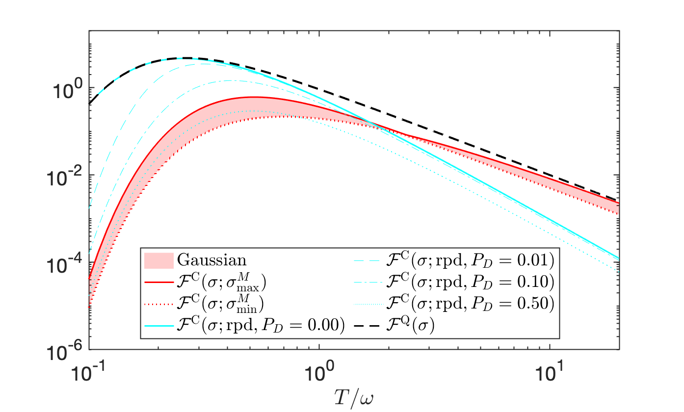
In Figure 2 the Fisher information of Gaussian measurements is depicted versus temperature. We compare this to the quantum Fisher information. Unlike in the high-temperature regime, where Gaussian measurements (Heterodyne specifically) are close to optimal, at low temperatures they perform rather poorly. In Section 3.3 we will see that on/off photo-detection measurements are a viable alternative in this latter case, and specifically that they perform close to optimal at low temperatures.
3.2.6 Optimal Gaussian measurements on multimode systems
When dealing with a multimode scenario, the problem becomes harder, and we were unable to derive an analytical solution. The main difficulty arises from the fact that the objective function to be optimised, i.e., the Fisher information, is a nonlinear function of the measurement covariance matrix. Nonetheless, one can design an algorithm to find the optimal measurement numerically. To begin with, one can use the fact that the covariance matrix of the optimal measurement is always pure and therefore belongs to the family of symmetric symplectic transformations, i.e., , where is a symmetric symplectic transformation, by definition. We can then run an optimisation program, e.g., “fmincon” on MATLAB programing language, to maximise —alternatively to minimise -—subject to the constraint that . See the appendix for an example code.
3.2.7 Multimode Gaussian states at thermal equilibrium: Local versus global Gaussian measurements

If the system is at thermal equilibrium, one can always diagonalise its covariance matrix by means of some temperature-independent symplectic transformation—i.e., to write it in the normal-mode basis. The symplectic transformation is a Gaussian process, and can be considered as part of the Gaussian measurement which we will optimise anyway. Therefore, we can focus only on initial thermal states with an uncorrelated covariance matrix . As for the measurement, one can first perform a joint Gaussian symplectic transformation on all modes—s.t., —and then perform a local Gaussian measurement . The idea is to find the optimal and .
Let us start by a scenario that only allows for local Gaussian measurements, i.e., . In this case, one can easily check that the classical Fisher information is additive, that is
| (46) |
Therefore, when we optimise over local Gaussian measurements, we have the optimal Fisher information
that is the sum of optimal Fisher information of individual modes. The question that remains to be answered is: can the performance of Gaussian measurements get better if we allow for joint measurements, i.e., if ?
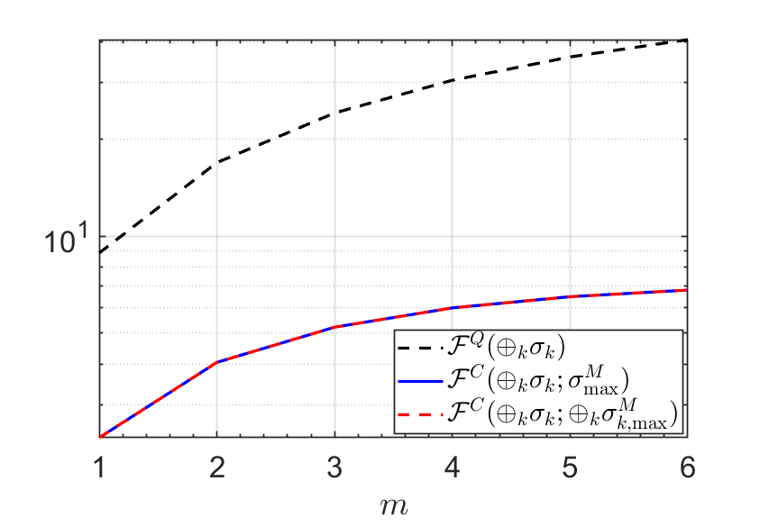
As depicted in Fig. 3, the global Gaussian measurements can be seen as the operation of some joint Gaussian unitary on all modes—namely an -mode symplectic transformation—followed by local measurements. The question is then whether the joint Gaussian operation can be beneficial. Mathematically, we know that , since the local measurements are a subset of global ones. We now wonder whether this inequality is in fact an equality, i.e., if
| (47) |
Note that, if we were not restricted to Gaussian measurements and could perform arbitrary measurements, then the equality would always hold. This is so because in this case the optimal Fisher information would reduce to the quantum Fisher information, which is additive and can be achieved by locally optimal measurements, that is
| (48) |
with being the optimal joint measurement—that is not necessarily Gaussian—performed on all modes, while is the optimal local measurement—again not necessarily Gaussian—performed on mode .
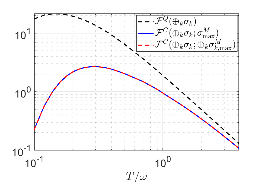
Unfortunately, we cannot prove the equivalence Eq. (47) in the general case. However, in the appendix we prove it analytically when all modes have identical covariance matrices—i.e., when . Furthermore, our numerical simulations support the equivalence for arbitrary product states. Based on these observations we conjecture this is generally true, however, a rigorous proof is missing currently.
3.3 On/Off Photo-Detection
Another type of measurement that will be shown to be relevant for thermometry and which can be of interest for experimental implementation is on/off photo-detection. This is a 2-outcome (detected or not detected) measurement and therefore it is not Gaussian. However, a link can be made between this type of photon-detection’s POVM elements and the POVM elements of a Gaussian measurement, characterized in Section 2. In what follows we consider realistic photo-detection, in which we allow for a probability of random counts—see e.g., [Rahimi-Keshari et al.(2016)Rahimi-Keshari, Ralph, and Caves, Barnett et al.(1998)Barnett, Phillips, and Pegg] for the error sources contributing to the random counts. For a single-mode system the POVM elements can then be written as
| (49) |
where is merely the vacuum state, and is the identity operator in the Hilbert space of the quantum system (not to be mistaken with ). The vacuum itself is a pure Gaussian state with a CM equal to identity and null displacement vector. The probability of finding any Gaussian system—with density matrix , covariance matrix and a vanishing displacement vector—in vacuum is then given by
| (50) |
where we use Eq. (2.1.1). Of course we also find the probablity of detection to be . The Classical Fisher Information associated to this probability distribution can be simply found from (3) and reads
| (51) |
As an example, we can use on/off photo-detection for thermometry of a single mode at thermal equilibrium, with . Using (3.3) one finds with . Thus the Fisher information is given by
| (52) |
In Fig. 2 we plot the classical Fisher information of realistic on/off photo-detection for various , and benchmark it against the optimal measurement and the optimal Gaussian measurement. Ideal on/off photo-detection performs close to optimal specifically at low temperatures. However, as soon as detection error is introduced and , the optimality at low temperatures is lost. The intuition behind this type of measurement being optimal is as follows: Firstly, we note that at thermal equilibrium the optimal measurement is in the basis of Hamiltonian, i.e., projection in the number basis. Secondly, at very low the system is basically frozen in its lowest energy eigenstates, namely it is in the vacuum state with some probability of populating the first excited state. As such, the projection in the number basis can be well approximated by ideal on/off photo-detection. Since the probability of observing the system in an excited state is already very low, then any random count will hugely impact our statistics and therefore realistic on/off photo-detection will eventually fail to estimate low enough temperatures. This argument can be made rigorous mathematically as well. At low temperature, one can see
| (53) |
Note that the exponential term in the case vanishes more rapidly, which is why realistic on/off photo-detection performs far from optimal for small enough . Moreover, by using Eq. (45) one can confirm that the leading order of quantum Fisher information at has the same value as the idealized detection, i.e., to the leading order .
3.3.1 Multimode photo-detection
For general m-mode systems, we can perform on/off photo-detection individually on each mode. The POVM elements can then be written as tensor product where . In what follows, we use to denote the vector of all zeros, to denote the vector of all zeros except the th element being , to denote the vector of all zeros except elements and which are and so on. Given an -mode Gaussian system with the covariance matrix , the probability of finding, for example, all modes in the vacuum state is (recall that all first moments of the system vanish)
| (54) |
where is the probability of random count for mode , and is the identity matrix. Similarly, by using , the probability of finding the th mode in an excited state while all the other modes at vacuum reads
| (55) |
where, for any covariance matrix , the operation is understood as eliminating the rows and columns associated to the mode . Following similar steps one can find the probability of other outcomes as well. However, one can restrict to a simplified version of on/off photo-detection with POVM elements, , and . One can consider yet simpler version, in which one does not distinguish what mode is excited therefore we have only three POVM elements with while the other two elements remain the same. These simplified versions should be fairly comparable to the non-simplified version at low temperatures, because at these temperatures the other POVM elements should not play a significant role anyway.
4 Conclusions
The problem of thermometry of Gaussian states with experimentally feasible measurements was addressed. The classical Fisher information of Gaussian measurements was charachterized. Finding the best Gaussian measurement can be expressed as an optimisation problem in which one looks for a pure covariance matrix that maximises the classical Fisher information (3.2.2). This may be done numerically in general. For thermal states one may find analytical solutions. In particular, for single-mode states at thermal equilibrium the optimal Gaussian measurement was found analytically to be either Homodyne or Heterodyne detection depending on the temperature. This is unlike the optimal non-Gaussian measurement, which is always a projection in the eigenbasis of the Hamiltonian of the system, regardless of the temperature. For a multimode scenario at thermal equilibrium we conjecture that the optimal Gaussian measurement is composed of a Gaussian unitary that brings the system into its normal modes basis, followed by a local optimal measurement on each of the normal modes. The proof of this is equivalent to proving Eq. (47), which remains an open question. Our numerical results support this conjecture, and we have proven this analytically for a scenario with all normal modes being equal.
We further compare the performance of the Gaussian measurements as well as photo-detection-like measurements with the quantum Fisher information, for systems at thermal equilibrium. We see that at low temperatures on/off photo-detection-like measurements perform almost optimally, whereas at high temperatures Gaussian measurements are close to optimal and saturate the quantum Cramér-Rao bound. We expect that for systems that are out of thermal equilibrium these results do not hold. For example, it is shown in [Correa et al.(2017)Correa, Perarnau-Llobet, Hovhannisyan, Hernández-Santana, Mehboudi, and Sanpera, Khan et al.(2022)Khan, Mehboudi, Terças, Lewenstein, and Garcia-March, Mehboudi et al.(2019b)Mehboudi, Lampo, Charalambous, Correa, García-March, and Lewenstein] that at ultracold temperatures and for non-equilibrium systems, sometimes position measurement—which is a Gaussian measurement—is optimal. A deeper investigation in this direction will be the be subject of future works.
Lastly, it would be interesting to consider the problem of thermometry with Gaussian measurements in the context of the Bayesian formalism, which has been the subject of few recent works [Rubio et al.(2021)Rubio, Anders, and Correa, Mehboudi et al.(2022)Mehboudi, Jorgensen, Seah, Brask, Kołodyński, and Perarnau-Llobet, Jorgensen et al.(2022)Jorgensen, Kołodyński, Mehboudi, Perarnau-Llobet, and Brask, Alves and Landi(2022)]. In particular, since the optimal Gaussian measurement is temperature dependent, this adds an extra challenge into designing optimal thermometry protocols when initial uncertainty about the true temperature is non negligible.
Acknowledgements
We are thankful to S. Rahimi-Keshari, F. Bakhshinezhad, J. Kolodynski, P. Sekatski, D. Rusca, and H. Zbinden for constructive discussions. This work was supported by Swiss National Science Foundation NCCR SwissMAP, the Government of Spain (FIS2020-TRANQI, ConTrAct FIS2017-83709-R, and Severo Ochoa CEX2019-000910-S), Fundacio Cellex, Fundacio Mir-Puig, Generalitat de Catalunya (CERCA, AGAUR SGR 1381 and QuantumCAT), the ERC AdG CERQUTE, the AXA Chair in Quantum Information Science. This project has received funding from the “Presidencia de la Agencia Estatal de Investigación” within the “Convocatoria de tramitación anticipada, correspondiente al año 2020, de las ayudas para contratos predoctorales (Ref. PRE2020-094374 PhD Fellowship) para la formación de doctores contemplada en el Subprograma Estatal de Formación del Programa Estatal de Promoción del Talento y su Empleabilidad en I+D+i, en el marco del Plan Estatal de Investigación Científica y Técnica y de Innovación 2017-2020, cofinanciado por el Fondo Social Europeo”. LL acknowledges support from Alexander von Humboldt Stiftung/Foundation. \onecolumngrid
Appendix A More about Gaussian measurements
In this Appendix we present some of the details of the toolboxes that were used in the main text. Please note that these results are only presented for self-containment and are not our original contributions.
A.1 General form of Gaussian measurements
In general, Gaussian measurements can be performed over an output state of any Gaussian map on the system , which is in general not a pure state, and will then be represented by more general POVM elements that read [Holevo(2019), Kiukas and Schultz(2013), Simon et al.(1994)Simon, Mukunda, and Dutta]
| (56) |
where the complete positivity condition must hold. The outcome probabilities of this Gaussian measurement are then given by
| (57) | ||||
| (58) |
where we have defined and . Integration gives
| (59) |
The previous scenario is revived by choosing and .
A.2 Local Gaussian measurements, reduced states and covariance matrices
Suppose we have a multi-mode state and we perform a Gaussian measurement on a subsystem. What is the post measurement state of the remaining modes? In principle, after performing some POVM on the system and observing an outcome associated with the element , the post measurement state is—up to a unitary—described by the density matrix
| (60) |
Despite the unitary freedom in the post measurement state, the reduced state of the modes over which we did not perform the measurement is independent of this unitary.
Suppose we have a two-party density operator, , of modes, where party has access to the first modes and party has the remaining modes. A POVM measurement is performed on part . That is, the overall POVM elements are given by . Given that we observe the result , the post-measurement [reduced] state of party reads
| (61) |
We are interested in knowing the covariance matrix of this reduced state. To this aim, we need to find the characteristic function, from which one can identify the covariance matrix.
Characteristic function of the reduced density matrix
By definition, we have
| (62) |
Let us focus on the numerator since the denominator is only a normalisation factor independent of . By noting that , this can be written as
| (63) |
where we denote , and . We can expand both and in terms of the displacement operator by using Eq. (2), such that
| (64) |
where is the number of modes over which we performed the measurement. Thus we can find the characteristic function of using the above expression
| (65) |
where we used that . Let us denote with and the covariance matrix and the displacement vectors of and , respectively. Therefore
| (66) | |||
| (67) |
with , and . The integral can also be evaluated using (2.1.1), which leads to
| (68) |
For simplicity let us assume that . Then we have
| (69) |
We can now simply find the post-measurement covariance matrix of party after the Gaussian measurement of party by setting in the exponent of the above relation, and by noticing that the covariance matrix of the measurement operator can be written as . Using the fact that
| (70) |
we have
| (71) |
in which is the correlation block of the covariance matrix , such that
| (74) |
Thus, the covariance matrix of , after ’s measurement is independent of the outcome and reads
| (75) |
One can check that the same result holds for . See Refs. [Giedke and Ignacio Cirac(2002), Genoni et al.(2016)Genoni, Lami, and Serafini] for earlier derivations.
Appendix B The classical Fisher information of Gaussian probability distributions
Given a Gaussian probability distribution which can be written as
| (76) |
we want to find the classical Fisher information. Note that we are assuming that the displacement vector is zero. Similar results are expected if the displacement vector is non zero, but is independent of the parameter. If neither of these are the case, one should use a more compete version of the Fisher information that is given in Eq. (3.2.2)—see also refs. [Monras(2013), Malagò and Pistone(2015)]. Let us define . Firstly, note that
| (77) |
where summation over repeated indices is understood. Recall the Jacobi’s formula for the derivative of determinant of [symmetric] matrices
| (78) | ||||
| (79) |
By substitution in the expression of classical Fisher information one gets
| (80) |
where we benefited multiple uses of , and also
| (81) |
Appendix C The maximum likelihood estimator
In this Appendix, through an example we provide details on how one can actually process experimental outcomes to assign an estimate to the unknown parameter—namely temperature. In local parameter estimation the maximum likelihood estimator (MLE) is known to saturate the Cramér-Rao bound [Paris(2009)]. In global estimation strategies, however, the MLE saturates the bound in the asymptotic limit of large number of repetitions of the measurement. Nonetheless, it is well-know that the MLE can saturate the bound when the outcome probability distribution is described by the “Gaussian family”—see e.g., section 3.1.2.4 of [Kolodynski(2014)] and references therein. This is indeed the case for our Gaussian measurements.
The Likelihood function is defined as the probability of observing the outcome “” if we performed some measurement on the state . By using Eq. (2.1.1) we have
| (82) |
The MLE, assigns the estimate to the unknown parameter that maximises the likelihood or the log likelihood. That is
| (83) |
By using the Jacobie’s formula for derivative of the determinant, and the formula for derivative of inverse matrix, this condition reduces to
| (84) |
Now let’s consider a single mode scenario in which the measurement is Homodyne detection with . In this case, we are projecting the state into the first quadrature. The above condition reduces to
| (85) |
which is quite expected.
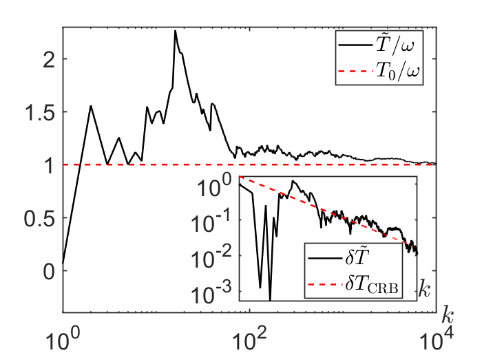
In order to convert this to a temperature estimate, we can use the parameter dependence of . As a relevant example, when the state is at thermal equilibrium, we have . As such, upon observing some outcome “”, we assign the following estimate to the temperature
| (86) |
Similarly, if we repeat the measurement times, we have
| (87) |
with the angled brackets in being the average over the measurement repetitions. In Fig. 4 we demonstrate a simulation of thermometry of a single mode thermal state by using Homodyne detection. One can observe how the estimate gets closer and closer to the true value of the temperature as we increase —a direct result of the central limit theorem. Moreover, one can see that the estimation error follows the trend of the Cramér-Rao bound.
Appendix D Imperfect Homodyne detection
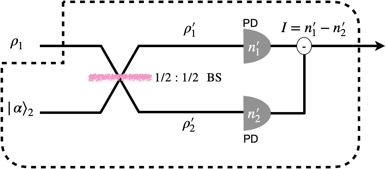
Following [Braunstein(1990)], we note that measuring the quadratures may be implemented by Homodyne detection, that is by interfering the signal and a local oscillator through a balanced beam splitter. The output modes will be photodetected and the currents will be subtracted (see Fig. 5). Perfect quadrature measurement requires a signal that has infinite energy. In many practical situations, the energy of the local oscillator is orders of magnitude higher than the signal which leads to very precise quadrature measurement—see e.g., [Lodewyck(2006)]. Nonetheless, in theory it is not be possible to have unlimited energy; and one can study its impact on the measurement precision. Below we examine the correction due to finite energy.
Firstly, note that the beam splitter is a Gaussian operation which can be represented by the following symplectic transformation
| (90) |
where represents the identity matrix. The beam splitter transforms the quadratures as follows
| (95) |
with the first two quadrature representing the signal, and the second two representing the local oscillator. For a balanced beam splitter we have which leads to
| (98) |
which transforms the quadratures as follows
| (103) |
The operator that represents the difference of the photocurrents from the two arms is given by
| (104) |
where we defined the number operators and similarly . Note that this operator is generally not Gaussian. Nonetheless, we note that by choosing the local oscillator such that we have
| (105) |
which up to a constant reproduces the first moment statistics of the position quadrature. However, as we saw in Appendix C, the estimator for thermometry is built upon the second moment, and thus plays the most crucial role in quality of Homodyne detection for thermometry at thermal equilibrium. For the second moment, we have
| (106) |
where we used and we assumed the local oscillator has a diagonal covariance matrix, i.e., .
In the last equation, we have some extra terms in that contain information about the momentum quadrature. To get rid of them, we prepare the local oscillator in a coherent state with the covariance matrix and with the displacement . We have
| (107) |
where we used that . Equations (105) and (107) suggest that has the same mean value as the position quadrature , while its variance is modified by an additional . In the limit of we can reproduce the quadrature statistics perfectly by using . However, this requires the local oscillator to have infinite energy. Nonetheless, for any situation that , we can still have a good approximation—in such a case our estimate for temperature will have a bias that is proportional to . While for local metrology schemes one can correct this bias (since we can exactly calculate it), for global thermometry protocols this is not possible.
Appendix E Additivity of the Gaussian-measured Fisher information in a special case
Proposition 1.
Let be a single-mode covariance matrix, and assume that and are both proportional to the identity. Then for all it holds that
| (108) |
where the optimization on the left-hand side is over all (multimode) covariance matrices of the measurement .
Proof.
Let be an arbitrary covariance matrix of an -mode Gaussian pure state. Then the spectrum of is well known to be of the form , where . Thus,
Hence, maximizing over , that is to say, maximizing over all choices of subjected to the above constraints, we obtain that
This establishes the additivity of the Gaussian-measured Fisher information in this special case. ∎
Appendix F Numerical optimisation, and the algorithm
We aim to identify the measurement CM that maximises (3.2.2). We are dealing with a nonlinear optimisation problem subject to the positive semi-definiteness criterion . We already proved that we should have , with some symplectic transformation satisfying . One can find the optimal in MATLAB by using the code at the end of this section. Notice that this algorithm works for arbitrary parameter estimation problem and is not limited to thermometry. One just needs to replace “” with the derivative of the covariance matrix w.r.t. the parameter to be estimated.
F.1 Examples of the simulation
As we mentioned in the main text, our numerical simulations support the conjecture (47). Here, we present two such simulations: (i) a scenario with two modes with different frequencies for different temperatures, and (ii) a scenario with several oscillators, each with a different frequency but for a finxed temperature. As one can see in Fig. 6, in either of these simulations global Gaussian measurements have no advantage over local ones.
References
- [Mehboudi et al.(2019a)Mehboudi, Sanpera, and Correa] Mohammad Mehboudi, Anna Sanpera, and Luis A Correa. Thermometry in the quantum regime: recent theoretical progress. Journal of Physics A: Mathematical and Theoretical, 52(30):303001, jul 2019a. doi: https://doi.org/10.1088/1751-8121/ab2828.
- [De Pasquale and Stace(2018)] Antonella De Pasquale and Thomas M. Stace. Quantum thermometry. In Felix Binder, Luis A. Correa, Christian Gogolin, Janet Anders, and Gerardo Adesso, editors, Thermodynamics in the Quantum Regime: Fundamental Aspects and New Directions, pages 503–527. Springer International Publishing, Cham, 2018. doi: https://doi.org/10.1007/978-3-319-99046-0˙21.
- [Giovannetti et al.(2011)Giovannetti, Lloyd, and Maccone] Vittorio Giovannetti, Seth Lloyd, and Lorenzo Maccone. Advances in quantum metrology. Nature photonics, 5(4):222–229, 2011. doi: https://doi.org/10.1038/nphoton.2011.35.
- [Giovannetti et al.(2006)Giovannetti, Lloyd, and Maccone] Vittorio Giovannetti, Seth Lloyd, and Lorenzo Maccone. Quantum metrology. Phys. Rev. Lett., 96:010401, Jan 2006. doi: https://doi.org/10.1103/PhysRevLett.96.010401.
- [Tóth and Apellaniz(2014)] Géza Tóth and Iagoba Apellaniz. Quantum metrology from a quantum information science perspective. Journal of Physics A: Mathematical and Theoretical, 47(42):424006, oct 2014. doi: https://doi.org/10.1088/1751-8113/47/42/424006.
- [Correa et al.(2015)Correa, Mehboudi, Adesso, and Sanpera] Luis A. Correa, Mohammad Mehboudi, Gerardo Adesso, and Anna Sanpera. Individual quantum probes for optimal thermometry. Phys. Rev. Lett., 114:220405, Jun 2015. doi: https://doi.org/10.1103/PhysRevLett.114.220405.
- [Jorgensen et al.(2020)Jorgensen, Potts, Paris, and Brask] Mathias R. Jorgensen, Patrick P. Potts, Matteo G. A. Paris, and Jonatan B. Brask. Tight bound on finite-resolution quantum thermometry at low temperatures. Phys. Rev. Research, 2:033394, Sep 2020. doi: https://doi.org/10.1103/PhysRevResearch.2.033394.
- [Hovhannisyan et al.(2021)Hovhannisyan, J0rgensen, Landi, Alhambra, Brask, and Perarnau-Llobet] Karen V. Hovhannisyan, Mathias R. J0rgensen, Gabriel T. Landi, Álvaro M. Alhambra, Jonatan B. Brask, and Martí Perarnau-Llobet. Optimal quantum thermometry with coarse-grained measurements. PRX Quantum, 2:020322, May 2021. doi: https://doi.org/10.1103/PRXQuantum.2.020322.
- [Weedbrook et al.(2012)Weedbrook, Pirandola, García-Patrón, Cerf, Ralph, Shapiro, and Lloyd] Christian Weedbrook, Stefano Pirandola, Raúl García-Patrón, Nicolas J. Cerf, Timothy C. Ralph, Jeffrey H. Shapiro, and Seth Lloyd. Gaussian quantum information. Rev. Mod. Phys., 84:621–669, May 2012. doi: https://doi.org/10.1103/RevModPhys.84.621.
- [Lewenstein et al.(2007)Lewenstein, Sanpera, Ahufinger, Damski, Sen(De), and Sen] Maciej Lewenstein, Anna Sanpera, Veronica Ahufinger, Bogdan Damski, Aditi Sen(De), and Ujjwal Sen. Ultracold atomic gases in optical lattices: mimicking condensed matter physics and beyond. Advances in Physics, 56(2):243–379, 2007. doi: https://doi.org/10.1080/00018730701223200.
- [Lewenstein et al.(2012)Lewenstein, Sanpera, and Ahufinger] Maciej Lewenstein, Anna Sanpera, and Veronica Ahufinger. Ultracold Atoms in Optical Lattices: Simulating quantum many-body systems. Oxford University Press, 2012. doi: https://doi.org/DOI:10.1093/acprof:oso/9780199573127.001.0001.
- [Serafini(2017)] Alessio Serafini. Quantum continuous variables: a primer of theoretical methods. CRC press, 2017.
- [Diamanti and Leverrier(2015)] Eleni Diamanti and Anthony Leverrier. Distributing secret keys with quantum continuous variables: Principle, security and implementations. Entropy, 17(9):6072–6092, 2015. ISSN 1099-4300. doi: https://doi.org/10.3390/e17096072.
- [Navascués and Acín(2005)] Miguel Navascués and Antonio Acín. Securitybounds for continuous variables quantum key distribution. Phys. Rev. Lett., 94:020505, Jan 2005. doi: https://doi.org/10.1103/PhysRevLett.94.020505.
- [Monras(2013)] Alex Monras. Phase space formalism for quantum estimation of gaussian states. arXiv preprint arXiv:1303.3682, 2013. doi: https://doi.org/10.48550/arXiv.1303.3682.
- [Jiang(2014)] Zhang Jiang. Quantum fisher information for states in exponential form. Phys. Rev. A, 89:032128, Mar 2014. doi: https://doi.org/10.1103/PhysRevA.89.032128.
- [Nichols et al.(2018)Nichols, Liuzzo-Scorpo, Knott, and Adesso] Rosanna Nichols, Pietro Liuzzo-Scorpo, Paul A. Knott, and Gerardo Adesso. Multiparameter gaussian quantum metrology. Phys. Rev. A, 98:012114, Jul 2018. doi: https://doi.org/10.1103/PhysRevA.98.012114.
- [Mehboudi et al.(2019b)Mehboudi, Lampo, Charalambous, Correa, García-March, and Lewenstein] Mohammad Mehboudi, Aniello Lampo, Christos Charalambous, Luis A. Correa, Miguel Ángel García-March, and Maciej Lewenstein. Using polarons for sub-nk quantum nondemolition thermometry in a bose-einstein condensate. Phys. Rev. Lett., 122:030403, Jan 2019b. doi: https://doi.org/10.1103/PhysRevLett.122.030403.
- [Planella et al.(2022)Planella, Cenni, Acín, and Mehboudi] Guim Planella, Marina F. B. Cenni, Antonio Acín, and Mohammad Mehboudi. Bath-induced correlations enhance thermometry precision at low temperatures. Phys. Rev. Lett., 128:040502, Jan 2022. doi: https://doi.org/10.1103/PhysRevLett.128.040502.
- [Correa et al.(2017)Correa, Perarnau-Llobet, Hovhannisyan, Hernández-Santana, Mehboudi, and Sanpera] Luis A. Correa, Martí Perarnau-Llobet, Karen V. Hovhannisyan, Senaida Hernández-Santana, Mohammad Mehboudi, and Anna Sanpera. Enhancement of low-temperature thermometry by strong coupling. Phys. Rev. A, 96:062103, Dec 2017. doi: https://doi.org/10.1103/PhysRevA.96.062103.
- [Hovhannisyan and Correa(2018)] Karen V. Hovhannisyan and Luis A. Correa. Measuring the temperature of cold many-body quantum systems. Phys. Rev. B, 98:045101, Jul 2018. doi: https://doi.org/10.1103/PhysRevB.98.045101.
- [Mukherjee et al.(2019)Mukherjee, Zwick, Ghosh, Chen, and Kurizki] Victor Mukherjee, Analia Zwick, Arnab Ghosh, Xi Chen, and Gershon Kurizki. Enhanced precision bound of low-temperature quantum thermometry via dynamical control. Communications Physics, 2(1):1–8, 2019. doi: https://doi.org/10.1038/s42005-019-0265-y.
- [Martín-Martínez et al.(2013)Martín-Martínez, Dragan, Mann, and Fuentes] Eduardo Martín-Martínez, Andrzej Dragan, Robert B Mann, and Ivette Fuentes. Berry phase quantum thermometer. New Journal of Physics, 15(5):053036, may 2013. doi: https://doi.org/10.1088/1367-2630/15/5/053036.
- [Holevo(2011)] Alexander S. Holevo. Probabilistic and Statistical Aspects of Quantum Theory. Publications of the Scuola Normale Superiore. Scuola Normale Superiore, Pisa, Italy, 2011. doi: https://doi.org/10.1007/978-88-7642-378-9.
- [Barnett and Radmore(2002)] Stephen Barnett and Paul M. Radmore. Methods in Theoretical Quantum Optics. Oxford Series in Optical and Imaging Sciences. Clarendon Press, 2002. ISBN 9780198563617. doi: https://doi.org/10.1093/acprof:oso/9780198563617.001.0001.
- [Newey and McFadden(1994)] Whitney K. Newey and Daniel McFadden. Chapter 36 large sample estimation and hypothesis testing. 4:2111–2245, 1994. ISSN 1573-4412. doi: https://doi.org/10.1016/S1573-4412(05)80005-4.
- [Pinel et al.(2013)Pinel, Jian, Treps, Fabre, and Braun] O. Pinel, P. Jian, N. Treps, C. Fabre, and D. Braun. Quantum parameter estimation using general single-mode gaussian states. Phys. Rev. A, 88:040102, Oct 2013. doi: https://doi.org/10.1103/PhysRevA.88.040102.
- [Monras(2006)] Alex Monras. Optimal phase measurements with pure gaussian states. Phys. Rev. A, 73:033821, Mar 2006. doi: https://doi.org/10.1103/PhysRevA.73.033821.
- [Oh et al.(2019)Oh, Lee, Rockstuhl, Jeong, Kim, Nha, and Lee] Changhun Oh, Changhyoup Lee, Carsten Rockstuhl, Hyunseok Jeong, Jaewan Kim, Hyunchul Nha, and Su-Yong Lee. Optimal gaussian measurements for phase estimation in single-mode gaussian metrology. npj Quantum Information, 5(1):1–9, 2019. doi: https://doi.org/10.1038/s41534-019-0124-4.
- [Morelli et al.(2021)Morelli, Usui, Agudelo, and Friis] Simon Morelli, Ayaka Usui, Elizabeth Agudelo, and Nicolai Friis. Bayesian parameter estimation using gaussian states and measurements. Quantum Science and Technology, 6(2):025018, mar 2021. doi: https://doi.org/10.1088/2058-9565/abd83d.
- [Kundu et al.(2022)Kundu, McKay, and Mallik] Neel Kanth Kundu, Matthew R. McKay, and Ranjan K. Mallik. Machine-learning-based parameter estimation of gaussian quantum states. IEEE Transactions on Quantum Engineering, 3:1–13, 2022. doi: https://doi.org/10.1109/TQE.2021.3137559.
- [Giedke and Ignacio Cirac(2002)] Géza Giedke and J. Ignacio Cirac. Characterization of gaussian operations and distillation of gaussian states. Phys. Rev. A, 66:032316, Sep 2002. doi: https://doi.org/10.1103/PhysRevA.66.032316.
- [Williamson(1936)] John Williamson. On the algebraic problem concerning the normal forms of linear dynamical systems. American Journal of Mathematics, 58(1):141–163, 1936. ISSN 00029327, 10806377. doi: https://doi.org/10.2307/2371062.
- [Lami et al.(2017)Lami, Hirche, Adesso, and Winter] Ludovico Lami, Christoph Hirche, Gerardo Adesso, and Andreas Winter. From log-determinant inequalities to gaussian entanglement via recoverability theory. IEEE Transactions on Information Theory, 63(11):7553–7568, 2017. doi: https://doi.org/10.1109/TIT.2017.2737546.
- [Lampo et al.(2017)Lampo, Lim, García-March, and Lewenstein] Aniello Lampo, Soon Hoe Lim, Miguel Ángel García-March, and Maciej Lewenstein. Bose polaron as an instance of quantum Brownian motion. Quantum, 1:30, September 2017. ISSN 2521-327X. doi: https://doi.org/10.22331/q-2017-09-27-30.
- [Khan et al.(2022)Khan, Mehboudi, Terças, Lewenstein, and Garcia-March] Muhammad Miskeen Khan, Mohammad Mehboudi, Hugo Terças, Maciej Lewenstein, and Miguel Angel Garcia-March. Subnanokelvin thermometry of an interacting -dimensional homogeneous bose gas. Phys. Rev. Research, 4:023191, Jun 2022. doi: https://doi.org/10.1103/PhysRevResearch.4.023191.
- [Malagò and Pistone(2015)] Luigi Malagò and Giovanni Pistone. Information geometry of the gaussian distribution in view of stochastic optimization. page 150–162, 2015. doi: 10.1145/2725494.2725510.
- [Rahimi-Keshari et al.(2016)Rahimi-Keshari, Ralph, and Caves] Saleh Rahimi-Keshari, Timothy C. Ralph, and Carlton M. Caves. Sufficient conditions for efficient classical simulation of quantum optics. Phys. Rev. X, 6:021039, Jun 2016. doi: https://doi.org/10.1103/PhysRevX.6.021039.
- [Barnett et al.(1998)Barnett, Phillips, and Pegg] Stephen M. Barnett, Lee S. Phillips, and David T. Pegg. Imperfect photodetection as projection onto mixed states. Optics Communications, 158(1):45–49, 1998. ISSN 0030-4018. doi: https://doi.org/10.1016/S0030-4018(98)00511-2.
- [Rubio et al.(2021)Rubio, Anders, and Correa] Jesús Rubio, Janet Anders, and Luis A. Correa. Global quantum thermometry. Phys. Rev. Lett., 127:190402, Nov 2021. doi: https://doi.org/10.1103/PhysRevLett.127.190402.
- [Mehboudi et al.(2022)Mehboudi, Jorgensen, Seah, Brask, Kołodyński, and Perarnau-Llobet] Mohammad Mehboudi, Mathias R Jorgensen, Stella Seah, Jonatan B Brask, Jan Kołodyński, and Martí Perarnau-Llobet. Fundamental limits in bayesian thermometry and attainability via adaptive strategies. Physical Review Letters, 128(13):130502, 2022. doi: https://doi.org/10.1103/PhysRevLett.128.130502.
- [Jorgensen et al.(2022)Jorgensen, Kołodyński, Mehboudi, Perarnau-Llobet, and Brask] Mathias R. Jorgensen, Jan Kołodyński, Mohammad Mehboudi, Martí Perarnau-Llobet, and Jonatan B. Brask. Bayesian quantum thermometry based on thermodynamic length. Phys. Rev. A, 105:042601, Apr 2022. doi: https://doi.org/10.1103/PhysRevA.105.042601.
- [Alves and Landi(2022)] Gabriel O. Alves and Gabriel T. Landi. Bayesian estimation for collisional thermometry. Phys. Rev. A, 105:012212, Jan 2022. doi: https://doi.org/10.1103/PhysRevA.105.012212.
- [Holevo(2019)] Alexander S. Holevo. Quantum systems, channels, information. de Gruyter, 2019. doi: https://doi.org/10.1515/9783110273403.
- [Kiukas and Schultz(2013)] Jukka Kiukas and Jussi Schultz. Informationally complete sets of gaussian measurements. Journal of Physics A: Mathematical and Theoretical, 46(48):485303, nov 2013. doi: https://doi.org/10.1088/1751-8113/46/48/485303.
- [Simon et al.(1994)Simon, Mukunda, and Dutta] R. Simon, N. Mukunda, and Biswadeb Dutta. Quantum-noise matrix for multimode systems: U(n) invariance, squeezing, and normal forms. Phys. Rev. A, 49:1567–1583, Mar 1994. doi: 10.1103/PhysRevA.49.1567.
- [Genoni et al.(2016)Genoni, Lami, and Serafini] Marco G. Genoni, Ludovico Lami, and Alessio Serafini. Conditional and unconditional gaussian quantum dynamics. Contemporary Physics, 57(3):331–349, 2016. doi: https://doi.org/10.1080/00107514.2015.1125624.
- [Paris(2009)] Matteo G. A. Paris. Quantum estimation for quantum technology. International Journal of Quantum Information, 7(supp01):125–137, 2009. doi: https://doi.org/10.1142/S0219749909004839.
- [Kolodynski(2014)] Jan Kolodynski. Precision bounds in noisy quantum metrology. arXiv:1409.0535, 2014. doi: https://doi.org/10.48550/arXiv.1409.0535.
- [Braunstein(1990)] Samuel L. Braunstein. Homodyne statistics. Phys. Rev. A, 42:474–481, Jul 1990. doi: https://doi.org/10.1103/PhysRevA.42.474.
- [Lodewyck(2006)] Jérôme Lodewyck. Dispositif de distribution quantique de clé avec des états cohérents à longueur d’onde télécom. PhD thesis, Université Paris Sud-Paris XI, 2006. URL https://pastel.archives-ouvertes.fr/tel-00130680.
