Nonadiabatic geometric quantum computation with cat qubits via invariant-based reverse engineering

Abstract

We propose a protocol to realize nonadiabatic geometric quantum computation of small-amplitude Schrödinger cat qubits via invariant-based reverse engineering. We consider a system with a two-photon driven Kerr nonlinearity, which can generate a pair of dressed even and odd coherent states (i.e., Schrödinger cat states) for fault-tolerant quantum computations. An additional coherent field is applied to linearly drive a cavity mode, to induce oscillations between dressed cat states. By designing this linear drive with invariant-based reverse engineering, we show how to implement nonadiabatic geometric quantum computation with cat qubits. The performance of the protocol is estimated by taking into account the influence of systematic errors, additive white Gaussian noise, $1/f$ noise, and decoherence including photon loss and dephasing. Numerical results demonstrate that our protocol is robust against these negative factors. Therefore, this protocol may provide a feasible method for nonadiabatic geometric quantum computation in bosonic systems.

I Introduction

Quantum coherence and quantum entanglement are arguably the most fascinating properties of quantum mechanics [1, 2, 3, 4]. These are the main resources for quantum information processing [1, 5] and quantum technologies of second generation [6]. Their recent applications include: demonstrations of quantum advantage using superconducting programmable processors [7] or boson sampling with squeezed states of photons [4], a quantum communication network over 4,600 km [8], and quantum-enhanced gravitational-wave detectors using squeezed vacuum [9, 10, 11, 12]. As a very important subfield of quantum information processing, quantum computation has shown a potentially great power in solving many specific problems [13, 14]. In a practical implementation of quantum computation, quantum algorithms are usually (but not always, e.g., in quantum annealing) designed as a sequence of quantum gates. Therefore, high-fidelity quantum gates are essential elements of quantum computation. Unfortunately, experimental imperfections, including operational errors, parameter fluctuations, and environment-induced decoherence, may affect the desired dynamics, limiting the fidelities of quantum gates. The problem how to overcome these experimental imperfections has to be solved for the constructions of practical quantum computers.

Because geometric phases are determined by the global geometric properties of the evolution paths, geometric quantum computation [15, 16] has shown robustness against local parameter fluctuations over a cyclic evolution [16, 17, 18]. As an extension of geometric quantum computation, holonomic quantum computation [19, 20, 21] based on non-Abelian geometric phases can be used to construct a universal set of single-qubit gates and several two-qubit entangling gates. Early implementations of geometric quantum computation involve adiabatic evolutions to suppress transitions between different eigenvectors of the Hamiltonian. This makes the evolution slow, and decoherence may destroy these geometric gates [22, 23, 24, 25, 26].

To speed up the evolution, nonadiabatic geometric quantum computation (NGQC) [27, 28, 29] was proposed. Note that NGQC is also enabled by geometric phases, thus inheriting robustness against local parameter fluctuations. Moreover, compared with adiabatic geometric quantum computation [19, 20, 21], NGQC is faster because the evolution is beyond the adiabatic limit. In addition, NGQC is compatible with various quantum optimized control techniques, such as reverse engineering [30, 31, 32, 33] and single-shot-shaped pulses [34, 35, 36]. Such techniques provide flexible ways in designing evolution paths for NGQC, reducing the number of auxiliary levels and sensitivity to certain types of control errors [37]. Because of the above advantages of NGQC, in the past decades, robust quantum computation has been discussed in theory [38, 39, 40] and successfully demonstrated in experiments [41, 42, 43].

Recent research has shown [44, 45, 46] that encoding quantum information in logical qubits is promising to protect quantum computation from errors. For the realization of logical qubits, bosonic systems are promising candidates, which can be constructed by quantized fields in, e.g., resonators, mechanical oscillators, and superconducting Josephson junctions [47, 48, 49, 50, 51]. The Schrödinger cat states of bosons [52] have shown applications in quantum computation in the early 2000s [53, 54]. Subsequently, it has been shown that the Schrödinger cat states [55, 56, 57, 58, 59, 60] can be used to construct types of useful error-correction codes [61, 62, 63, 64, 65, 66, 67, 68, 69, 70, 71, 72, 73, 74, 75], providing protection against cavity dephasing [62, 66], and thus have attracted much interest.

Recently, based on cat codes, various protocols [50, 51, 76, 49, 47, 48, 59] for preparing, stabilizing, and manipulating cat qubits have been put forward. Moreover, quantum computation [50] and adiabatic geometric quantum control [66] of cat qubits have also been considered. However, so far, only a few protocols [66, 77] have been proposed to implement geometric computation using cat qubits. Because of the difficulty to arbitrarily manipulate a bosonic mode, it is still a challenge to realize NGQC using bosonic cat qubits, which are both robust and fault tolerant.

In this manuscript, we propose to use cat qubits to implement NGQC via invariant-based reverse engineering. To construct cat qubits, a two-photon driven Kerr nonlinearity is used to restrict the evolution of cavity modes to a subspace spanned by a pair of cat states. We apply an additional coherent field to linearly drive a cavity mode in order to induce oscillations between dressed cat states. With the control fields designed by invariant-based reverse engineering, the system can have a cycling evolution, which acquire only pure geometric phases. Hence, NGQC with cat qubits can be implemented.

An amplitude-amplification method, using light squeezing [78, 79], is applied to increase the distinguishability of different cat states, so that it can be easier to detect input and output states in practice. Moreover, two-qubit quantum gates of cat qubits are also considered by using couplings between two cavity modes. Controlled two-qubit geometric quantum gates can be implemented almost perfectly.

Finally, the performance of the protocol in the presence of systematic errors, additive white Gaussian noise (AWGN), $1/f$ noise, and decoherence (including photon loss and dephasing) are investigated via numerical simulations. Our results indicate that the protocol is robust against these negative factors.

The article is organized as follows. In Sec. II, we briefly introduce the basic theory for invariant-based NGQC. In Sec. III, we describe how to implement single- and two-qubit NGQC with cat qubits. In Sec. IV, we consider experimental imperfections and estimate the performance of the protocol via numerical simulations. In Sec. V, we introduce an amplification method based on quadrature squeezing for the amplitudes of cat states, so that the detection of input and output states can be performed easily. In Sec. VI, we discuss a possible implementation of our protocol using a superconducting quantum parametron. Finally, our conclusions are given in Sec. VII. Appendix A includes a derivation of a dynamic invariant and the choice of parameters for eliminating dynamical phases.

II Nonadiabatic geometric quantum computation based on a dynamic invariant

For details, we first recall the Lewis-Riesenfeld invariant theory [80]. Assuming that a physical system is described by a Hamiltonian $H(t)$, a Hermitian operator $I(t)$ satisfies the following equation $(\hbar=1)$

$$i\frac{\partial}{\partial t}I(t)-[H(t),I(t)]=0.$$ (1)

For a non-degenerate eigenvector $|\phi_{l}(t)\rangle$ of $I(t)$, $|\psi_{l}(t)\rangle=\exp[i\alpha_{l}(t)]\,|\phi_{l}(t)\rangle$ is a solution of the time-dependent Schrödinger equation $i|\dot{\psi}(t)\rangle=H(t)|\psi(t)\rangle$. Here, $\alpha_{l}(t)$ is the Lewis-Riesenfeld phase defined as

$$\alpha_{l}(t)=\int_{0}^{t}\langle\phi_{l}(\tau)|\left[i\frac{\partial}{\partial\tau}-H(\tau)\right]|\phi_{l}(\tau)\rangle d\tau.$$ (2)

To realize NGQC, one can select a set of time-dependent vectors, $\{|\phi_{l}(t)\rangle\}$, spanning a computational subspace $\mathcal{S}$. According to Ref. [81], $\{|\phi_{l}(t)\rangle\}$ should satisfy the three conditions: (i) the cyclic evolution condition $|\phi_{l}(0)\rangle=|\phi_{l}(T)\rangle$ with $T$ being the total operation time; (ii) the von Neumann equation

$$\dot{\Xi}_{l}(t)=-i[H(t),\Xi_{l}(t)],$$ (3)

with $\Xi_{l}(t)=|\phi_{l}(t)\rangle\langle\phi_{l}(t)|$; and (iii) annihilation of the dynamical phase

$$\vartheta_{l}(T)=-\int_{0}^{T}\langle\phi_{l}(t)|H(t)|\phi_{l}(t)\rangle\,dt=0.$$ (4)

When satisfying the three conditions, the evolution in subspace $\mathcal{S}$ can be described by

$$U(T,0)=\sum\limits_{l}\exp[i\Theta_{l}(T)]\,\Xi(0),$$ (5)

with a pure geometric phase

$$\Theta_{l}(T)=\int_{0}^{T}\langle\phi_{l}(t)|i\frac{\partial}{\partial t}|\phi_{l}(t)\rangle\,dt.$$ (6)

Ref. [82] has shown that, a non-degenerate eigenvector $|\phi_{l}(t)\rangle$ of an invariant obeys the von Neumann equation given in Eq. (3). Therefore, when the parameters of $I(t)$ are designed with the cycling boundary conditions and the dynamical part of the Lewis-Riesenfeld phase is eliminated, the three conditions are satisfied. In this case, one can implement NGQC with a dynamic invariant $I(t)$.

III Nonadiabatic geometric quantum computation of cat qubits

III.1 Arbitrary single-qubit gates

III.1.1 Hamiltonian and evolution operator of a single resonator

We consider a resonant single-mode two-photon (i.e., quadrature) squeezing drive applied to a Kerr-nonlinear resonator. In the frame rotating at the resonator frequency $\omega_{1}$, the system is described by the Hamiltonian [51, 49]

$$H_{\mathrm{cat}}=-Ka_{1}^{{\dagger}2}a_{1}^{2}+\epsilon_{2}\left(e^{2i\xi}a_{1}^{{\dagger}2}+e^{-2i\xi}a_{1}^{2}\right),$$ (7)

where $K$ is the Kerr nonlinearity, $a_{1}$ ($a_{1}^{\dagger}$) is the annihilation (creation) operator of the resonator (cavity) mode, $\epsilon_{2}$ is the strength of the two-photon drive assumed here to be real, and $\xi$ is its phase. The coherent states $|\pm\alpha\rangle_{1}$ (where $\alpha=\sqrt{\epsilon_{2}/K}e^{i\xi}$ is the complex amplitude) are two degenerate eigenstates of $H_{\mathrm{cat}}$. Therefore, the even ($|\mathcal{C}_{+}\rangle_{1}$) and odd ($|\mathcal{C}_{-}\rangle_{1}$) coherent states, often referred to as Schrödinger cat states, which are defined as

$$|\mathcal{C}_{\pm}\rangle_{1}=\frac{1}{\sqrt{\mathcal{N}_{\pm}}}\left(|\alpha\rangle_{1}\pm|-\alpha\rangle_{1}\right),$$ (8)

are two orthonormal degenerate eigenstates of $H_{\mathrm{cat}}$, where $\mathcal{N}_{\pm}=2[1\pm\exp(-2|\alpha|^{2})]$ are the normalized coefficients. The total Hamiltonian

$$H_{\rm{tot}}(t)=H_{\mathrm{cat}}+H_{c},$$ (9)

includes a control Hamiltonian defined as [51]

$$H_{c}(t)=\chi(t)a_{1}^{\dagger}a_{1}+\epsilon(t)a_{1}^{\dagger}+\epsilon^{*}(t)a_{1},$$ (10)

with $\chi(t)$ and $\epsilon(t)$ being the detuning and strength of a single-photon drive, respectively.

When the energy gap $E_{\mathrm{gap}}$ between the cat states $|\mathcal{C}_{\pm}\rangle_{1}$ and their nearest eigenstate of $H_{\mathrm{cat}}$ is much larger than $\chi(t)$ and $\epsilon(t)$, the system can be restricted to the subspace $\mathcal{S}$ spanned by $|\mathcal{C}_{\pm}\rangle_{1}$. We can accordingly use the cat states to define the Pauli matrices as

$$\sigma_{x} =\sigma_{+}+\sigma_{-},\ \ \ \ \ \ \ \ \ \sigma_{y}=i(\sigma_{-}-\sigma_{+}),$$ (11)

$$\sigma_{z} =\sigma_{+}\sigma_{-}-\sigma_{-}\sigma_{+},\ \ \ \vec{\sigma}=(\sigma_{x},\sigma_{y},\sigma_{z}),$$ (12)

in terms of the raising ($\sigma_{+}$) and lowering ($\sigma_{-}$) qubit operators,

$$\sigma_{+}=|\mathcal{C}_{+}\rangle_{1}\langle\mathcal{C}_{-}|,\ \ \ \ \sigma_{-}=|\mathcal{C}_{-}\rangle_{1}\langle\mathcal{C}_{+}|$$ (13)

Then, the Hamiltonian of the system can be simplified to $H_{c}(t)=\vec{\Omega}(t)\cdot\vec{\sigma}$, where, $\vec{\Omega}(t)=[\Omega_{x}(t),\Omega_{y}(t),\Omega_{z}(t)]$ is a set of driving amplitudes to be determined. We find that $I(t)=\vec{\zeta}(t)\cdot\vec{\sigma}$ is a dynamic invariant, where $\vec{\zeta}(t)=[\zeta_{x}(t),\zeta_{y}(t),\zeta_{z}(t)]$ is the three-dimensional time-dependent vector satisfying the conditions $\dot{\vec{\zeta}}(t)=2\vec{\Omega}(t)\times\vec{\zeta}(t)$ and $|\vec{\zeta}(t)|=\mathrm{const}$ (see Appendix A for details). The three components $[\zeta_{x}(t),\zeta_{y}(t),\zeta_{z}(t)]$ of $\vec{\zeta}(t)$ denote the projections of the dynamic invariant $I(t)$ along the directions $(\sigma_{x},\sigma_{y},\sigma_{z})$ in the SU(2) algebra.

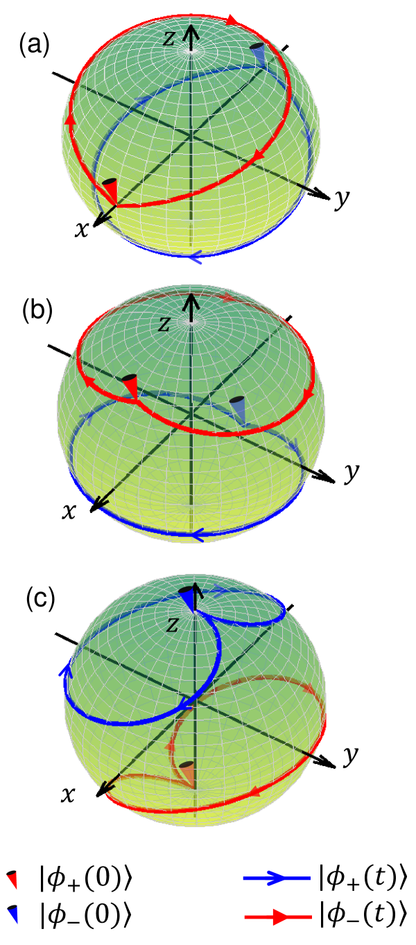
Figure 1: Trajectories of the eigenvectors $|\phi_{+}(t)\rangle$ (red-solid curve) and $|\phi_{-}(t)\rangle$, defined in Eq. (14), on the Bloch sphere in the implementations of (a) the NOT gate, (b) the Hadamard gate, and (c) the $\pi$-phase gate. Parameters are listed in Table 1.

By introducing two time-dependent dimensionless parameters $\eta$ and $\mu$, we can parametrize $\vec{\zeta}(t)$ as $(\sin{\eta}\sin{\mu},\cos{\eta}\sin{\mu},\cos{\mu})$ and the eigenvectors of the dynamic invariant $I(t)$ can be derived as

$$|\phi_{+}(t)\rangle=\cos\frac{\mu}{2}|\mathcal{C}_{+}\rangle_{1}+i\exp(-i\eta)\sin\frac{\mu}{2}|\mathcal{C}_{-}\rangle_{1},$$ (14)

$$|\phi_{-}(t)\rangle=i\exp(i\eta)\sin\frac{\mu}{2}|\mathcal{C}_{+}\rangle_{1}+\cos\frac{\mu}{2}|\mathcal{C}_{-}\rangle_{1}.$$ (15)

We can design the parameters $\epsilon(t)$ and $\chi(t)$ as

$$\mathrm{Re}[\epsilon(t),\xi]= ~{}\frac{\sqrt{\mathcal{N}_{+}\mathcal{N}_{-}}}{8\alpha}\left(\Omega_{x}\cos\xi+e^{2|\alpha|^{2}}\Omega_{y}\sin\xi\right),$$ (16)

$$\mathrm{Im}[\epsilon(t),\xi]= ~{}\mathrm{Re}[\epsilon(t),\xi-\pi/2],$$ (17)

$$\chi(t)= ~{}\frac{(\dot{\eta}\sin^{2}\mu)\mathcal{N}_{+}\mathcal{N}_{-}}{[(\mathcal{N}_{+}^{2}-\mathcal{N}_{-}^{2})|\alpha|^{2}]},$$ (18)

with effective driving amplitudes (see Appendix A for details)

$$\Omega_{x}= ~{}\frac{1}{2}\left[{\dot{\eta}}\sin\eta\sin(2\mu)-2\dot{\mu}\cos\eta\right],$$ (19)

$$\Omega_{y}= ~{}\frac{1}{2}\left[{\dot{\eta}}\cos\eta\sin(2\mu)+2\dot{\mu}\sin\eta\right].$$ (20)

Both dynamical phases, acquired by the eigenvectors shown in Eq. (14), vanish due to $\langle\phi_{\pm}(t)|H_{c}(t)|\phi_{\pm}(t)\rangle=0$, while the geometric phases acquired by $|\phi_{\pm}(t)\rangle$, defined in Eq. (14), are

$$\Theta_{\pm}(t) \equiv~{}\int_{0}^{t}\langle\phi_{\pm}(\tau)|i\frac{\partial}{\partial\tau}|\phi_{\pm}(\tau)\rangle d\tau$$ (21)

$$=~{}\pm\int_{0}^{t}\dot{\eta}\sin^{2}\left(\frac{\mu}{2}\right)d\tau.$$ (22)

According to Eq. (5), the evolution of the system in the subspace $\mathcal{S}$, after a cycling evolution with period $T$, is calculated as

$$U_{s}(T,0)=\exp\left[i\theta\vec{\zeta}(0)\cdot\vec{\sigma}\right]$$ (23)

$$= \left[\begin{array}[]{cccc}\cos\theta+i\cos\mu_{0}\sin\theta&\exp(i\eta_{0})\sin\mu_{0}\sin\theta\\ -\exp(-i\eta_{0})\sin\mu_{0}\sin\theta&\cos\theta-i\cos\mu_{0}\sin\theta\\ \end{array}\right],\ \ \$$ (26)

where $\theta=\int_{0}^{T}\dot{\eta}\sin^{2}(\mu/2)\,dt$ is the final geometric phase of the cycling evolution, and $\mu_{0}$ ($\eta_{0}$) is the initial value of $\mu$ ($\eta$). The evolution operator $U_{s}(T,0)$ represents a rotation on the Bloch sphere that can generate arbitrary single-qubit gates [83, 84]. For a cycling evolution, the parameters can be interpolated by trigonometric functions as

$$\mu= ~{}\mu_{0}+\Lambda\sin^{2}\left(\frac{\pi t}{T}\right),$$ (27)

$$\eta= ~{}\eta_{0}+\pi\left[1-\cos\left(\frac{\pi t}{T}\right)\right],$$ (28)

where $\Lambda$ is an auxiliary parameter to be determined according to the requirements of different gates.

III.1.2 Examples of single-qubit-gate implementations

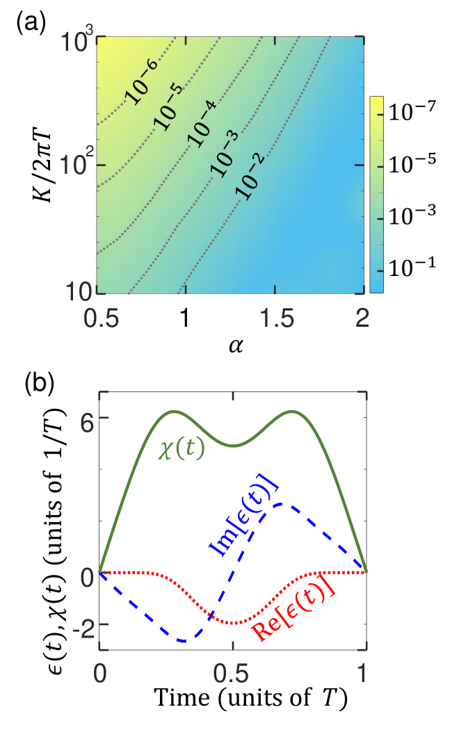
Figure 2: (a) Infidelity $(1-\bar{F}_{\rm{NOT}})$ versus the amplitude $\alpha$ and the Kerr nonlinearity $K$ for our implementation of the NOT gate. (b) Time variations of the parameters $\chi(t)$, $\mathrm{Re}[\epsilon(t)]$, and $\mathrm{Im}[\epsilon(t)]$, defined in Eq. (16). Parameters are listed in Table 1.

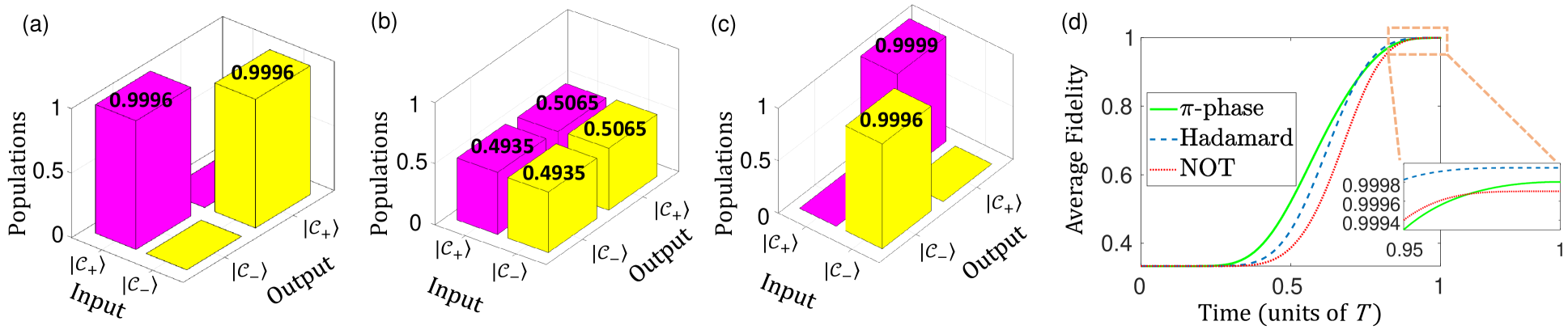
Figure 3: Populations of different output states for different input states in the implementation of: (a) the NOT gate, (b) the Hadamard gate, and (c) the $\pi$-phase gate with parameters $K=2\pi\times 12.5$ MHz and $|\alpha|=0.5$. (d) Average fidelities of the NOT gate (red-dotted curve), the Hadamard gate (blue-dashed curve), and the $\pi$-phase gate (green-solid curve) with parameters $K=2\pi\times 12.5$ MHz and $|\alpha|=0.5$.

We now discuss how to use the evolution operator $U_{s}(T,0)$, given in Eq. (23), to realize:

(i) the NOT gate, $U_{\rm{NOT}}=\sigma_{x}$;

(ii) the Hadamard gate, $U_{\mathrm{H}}=(\sigma_{z}+\sigma_{x})/\sqrt{2}$;

(iii) the arbitrary phase gate, $U_{\rm{Phase}}(\theta)=\cos{\frac{\theta}{2}}\cdot\mathbbm{1}+i\sin{\frac{\theta}{2}}\cdot\sigma_{z}$, where $\mathbbm{1}$ is the identity operator acting on the cat qubit.

To determine the initial values of $\mu_{0}$ and $\eta_{0}$, we can exploit the evolution operator $U_{s}(T,0)$ shown in Eq. (23). Because the system evolves through a cycling evolution [$|\phi_{\pm}(T)\rangle=|\phi_{\pm}(0)\rangle$], the evolution operator only relies on the acquired geometric phase $\theta$ and the initial values of $\mu_{0}$ and $\eta_{0}$. For example, to implement the NOT gate, we should make the diagonal elements of the evolution operator $U_{s}(T,0)$ in Eq. (23) to become zeros. Therefore, we set $\theta=\mu_{0}=\pi/2$. In addition, the off-diagonal elements of $U_{s}(T,0)$ should be equal to 1. Thus, we select $\eta_{0}=\pi/2$. Dropping a global phase $\pi/2$, $U_{s}(T,0)$ becomes the NOT gate

$$U_{\mathrm{NOT}}=\left[\begin{array}[]{cc}0&1\\ 1&0\\ \end{array}\right].$$ (29)

Moreover, to implement the Hadamard gate, the matrix for $U_{s}(T,0)$ should be equal to

$$U_{\mathrm{H}}=\frac{1}{\sqrt{2}}\left[\begin{array}[]{cc}1&1\\ 1&-1\\ \end{array}\right].$$ (30)

Comparing $U_{\mathrm{H}}$ and $U_{s}(T,0)$ in Eq. (23), we find that $\mu_{0}=\pi/4$ and $\eta_{0}=\theta=\pi/2$. In this case, up to a global phase $\pi/2$, $U_{s}(T,0)$ becomes the Hadamard gate.

Finally, for the $\pi$-phase gate, the off-diagonal elements of $U_{s}(T,0)$ should vanish. Therefore, we set $\mu_{0}=0$. In this case, $U_{s}(T,0)$ is independent of the value of $\eta_{0}$, so that we can choose $\eta_{0}=0$ for simplicity. Omitting the global phase $\theta$, $U_{s}(T,0)$ becomes

$$U_{\theta}=\left[\begin{array}[]{cc}1&1\\ 1&e^{-2i\theta}\\ \end{array}\right].$$ (31)

Then, the $\pi$-phase gate can be realized with $\theta=\pi/2$. For the sake of clarity, the corresponding parameters to realize the three gates for $\theta=\pi/2$ are listed in Table 1.

Table 1: Parameters for our implementations of single-qubit gates

gate	$\mu_{0}$	$\eta_{0}$	$\theta$	$\Lambda$
$U_{\rm{NOT}}$	$\pi/2$	$\pi/2$	$\pi/2$	$0.8089$
$U_{\mathrm{H}}$	$\pi/4$	$\pi/2$	$\pi/2$	$0.3859$
$U_{\rm{Phase}}(\pi)$	$0$	$0$	$\pi/2$	$1.4669$

According to the parameters given in Table 1, on the Bloch sphere in Fig. 1, we plot the trajectories of the eigenvectors $|\phi_{\pm}(t)\rangle$, i.e.,

$$\vec{r}_{\pm}(t)=\sum_{k=x,y,z}\mathrm{Tr}[|\phi_{\pm}(t)\rangle\langle\phi_{\pm}(t)|\sigma_{k}]\vec{e}_{k},$$ (32)

where $\vec{e}_{k}$ is the unit direction vector along the $k$-axis. As shown in each panel of Fig. 1, both vectors $|\phi_{\pm}(t)\rangle$ evolve along their cycling paths individually, and the geometric phases acquired by them are equal to half of the solid angles of the areas surrounded by the corresponding paths. In addition, the solid angles of the paths of $\vec{r}_{\pm}(t)$ have opposite signs, because the paths are on the upper and lower half spheres, respectively. These numerical results are in agreement with the theoretical results in Eq. (21).

The average fidelity of the gates over all possible initial states in the subspace $\mathcal{S}$ can be calculated by [85, 86]

$$\bar{F}_{G}=\frac{1}{\mathcal{D}(\mathcal{D}+1)}\left[\mathrm{Tr}(MM^{\dagger})+|\mathrm{Tr}(M)|^{2}\right],$$ (33)

with $M=\mathcal{P}_{c}U^{\dagger}_{G}U_{1}\mathcal{P}_{c}$, while $\mathcal{P}_{c}$ and $\mathcal{D}$ are the projector and dimension of the computational subspace, respectively. The subscript “$G$” denotes the desired gate, e.g., $G=\rm{NOT}$ when one wants to implement the NOT gate. Figure 2(a) shows the infidelity $(1-\bar{F}_{\rm{NOT}})$ versus the amplitude $\alpha$ and the Kerr nonlinearity $K$ for the NOT gate, as an example.

We find that the average fidelity $\bar{F}_{\rm{NOT}}$ decreases sharply when the amplitude $\alpha$ increases. This effect can be understood because the control parameters $\chi(t)$ and $\epsilon(t)$ increase with $\exp(|\alpha|^{2})$ according to Eq. (16). Consequently, the ratio between the energy gap and parameters of $H_{c}(t)$ reduces, and the leakage to other eigenstates of $H_{\rm{cat}}$ becomes significant. To manipulate the cat qubit with a larger $\alpha$, one may increase the Kerr-nonlinearity $K$ and the strength $\epsilon_{2}$ of the squeezing drive, but we should notice that $K$ and $\epsilon_{2}$ both have their upper limits in experiments [51]. We can also consider a longer interaction time $T$ to reduce values of the parameters in $H_{\mathrm{add}}(t)$, but such a long-time evolution may increase the influence of decoherence.

For a realistic value of the Kerr nonlinearity $K=2\pi\times 12.5$ MHz [51] ($E_{\mathrm{gap}}=161$ MHz), the parameters $\chi(t)$ and $\epsilon(t)$ are shown in Fig. 2(b), when the total interaction time $T=1~{}\mu$s and the amplitude of coherent states is $|\alpha|=0.5$. With these parameters, we obtain $\bar{F}_{\rm{NOT}}=0.9997$, indicating that the NOT gate can be implemented almost perfectly. To show the performance of different types of quantum gates, we plot the populations of different output states with different input states in the implementation of the NOT, Hadamard, and the $\pi$-phase gates in Figs. 3(a), 3(b), and 3(c), respectively. As shown, the populations of the output states are all very close to the ideal values of the theoretical results, and the leakage to unwanted levels is negligible.

For example, we calculate the final fidelities $F_{\mathrm{H}}(T)$ of the Hadamard gate with different input states. For the input state $|\mathcal{C}_{+}\rangle$, we obtain

$$\langle\mathcal{C}_{+}|U_{\mathrm{H}}(T)|\mathcal{C}_{+}\rangle=0.6773+0.2125i,$$ (34)

(35)

$$\langle\mathcal{C}_{-}|U_{\mathrm{H}}(T)|\mathcal{C}_{+}\rangle=0.6743+0.2036i,$$

resulting in

$$P_{+}(T)=|\langle\mathcal{C}_{+}|U_{\mathrm{H}}(T)|\mathcal{C}_{+}\rangle|^{2}=0.5039,$$ (36)

(37)

$$P_{-}(T)=|\langle\mathcal{C}_{-}|U_{\mathrm{H}}(T)|\mathcal{C}_{+}\rangle|^{2}=0.4961.$$

Moreover, for the input state $|\mathcal{C}_{+}\rangle$, the gate fidelity is

$$F_{\mathrm{H}}^{+}(T) = |\langle\Psi_{+}(T)|\mathcal{C}_{+}\rangle|^{2}$$ (38)

$$= \frac{1}{2}|\langle\mathcal{C}_{+}|U_{\mathrm{H}}(T)|\mathcal{C}_{+}\rangle+\langle\mathcal{C}_{-}|U_{\mathrm{H}}(T)|\mathcal{C}_{+}\rangle|^{2}$$

$$= 1-4.4480\times 10^{-5},$$

where

$$|\Psi_{+}(T)\rangle=U_{\mathrm{H}}(T)|\mathcal{C}_{+}\rangle=\frac{1}{\sqrt{2}}(|\mathcal{C}_{+}\rangle+|\mathcal{C}_{-}\rangle).$$ (42)

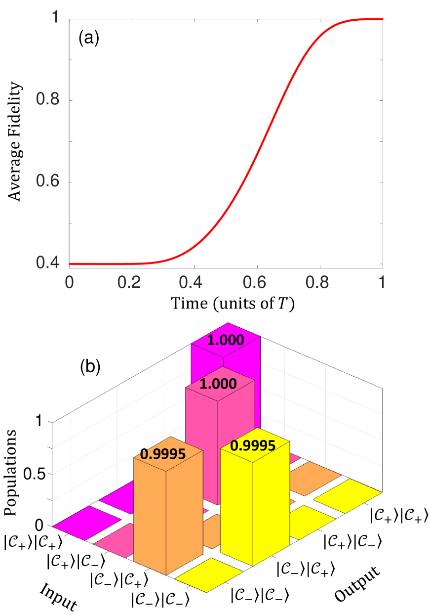
Figure 4: Implementation of the CNOT gate: (a) Time variation of the average fidelity $\bar{F}_{\mathrm{CNOT}}(t)$. (b) Populations of different output states for different input states.

For the input state $|\mathcal{C}_{-}\rangle$, we obtain

$$\langle\mathcal{C}_{+}|U_{\mathrm{H}}(T)|\mathcal{C}_{-}\rangle=0.6743+0.2036i,$$ (43)

(44)

$$\langle\mathcal{C}_{-}|U_{\mathrm{H}}(T)|\mathcal{C}_{-}\rangle=-0.6817-0.1978i,$$

resulting in

$$P_{+}^{\prime}(T)=|\langle\mathcal{C}_{+}|U_{\mathrm{H}}(T)|\mathcal{C}_{-}\rangle|^{2}=0.4961,$$ (45)

(46)

$$P_{-}^{\prime}(T)=|\langle\mathcal{C}_{-}|U_{\mathrm{H}}(T)|\mathcal{C}_{-}\rangle|^{2}=0.5039.$$

Accordingly, the gate fidelity in this case is

$$F_{\mathrm{H}}^{-}(T) = |\langle\Psi_{-}(T)|\mathcal{C}_{-}\rangle|^{2}$$ (47)

$$= \frac{1}{2}|\langle\mathcal{C}_{+}|U_{\mathrm{H}}(T)|\mathcal{C}_{-}\rangle-\langle\mathcal{C}_{-}|U_{\mathrm{H}}(T)|\mathcal{C}_{-}\rangle|^{2}$$

$$= 1-4.4752\times 10^{-5},$$

where

$$|\Psi_{-}(T)\rangle=U_{\mathrm{H}}(T)|\mathcal{C}_{-}\rangle=\frac{1}{\sqrt{2}}(|\mathcal{C}_{+}\rangle-|\mathcal{C}_{-}\rangle).$$ (51)

Therefore, the fidelities of the Hadamard gate for the two input states $|\mathcal{C}_{\pm}\rangle$ are both nearly unity.

In addition, we also plot the average fidelities of the NOT, Hadamard and $\pi$-phase gates in Fig. 3(d). The average fidelities of the three gates are $\bar{F}_{\rm{NOT}}=0.9997$, $\bar{F}_{\mathrm{H}}=0.9999$, and $\bar{F}_{\pi}=0.9998$, respectively. The results show that the three gates are implemented with very high fidelities.

III.1.3 Hamiltonian and evolution operator of two coupled resonators

Now we consider a generalized scheme when two cavity modes are driven by two Kerr-nonlinear resonators, as described by the Hamiltonian

$$H_{\mathrm{cat2}}=-K\sum_{n=1,2}a_{n}^{{\dagger}2}a_{n}^{2}+\epsilon_{2}(a_{n}^{{\dagger}2}+a_{n}^{2}).$$ (52)

The product coherent states $|\pm\alpha\rangle_{1}\otimes|\pm\alpha\rangle_{2}$ of the modes $a_{1}$ and $a_{2}$ are the four degenerate eigenstates of $H_{\mathrm{cat}2}$. Therefore, the product cat states $\{|\mathcal{C}_{\pm}\rangle_{1}\otimes|\mathcal{C}_{\pm}\rangle_{2}\}$ span a four-dimensional computational subspace $\mathcal{S}_{2}$ useful for implementing two-qubit gates.

Additionally, we consider a control Hamiltonian [47, 50, 87]

$$H_{c2}(t)= ~{}\chi_{12}(t)a_{1}^{{\dagger}}a_{1}a_{2}^{{\dagger}}a_{2}+a_{1}^{{\dagger}}a_{1}[\lambda^{*}(t)a_{2}+\lambda(t)a_{2}^{{\dagger}}]$$ (53)

$$+\tilde{\epsilon}^{*}(t)a_{2}+\tilde{\epsilon}(t)a_{2}^{\dagger}+\sum_{n=1,2}\chi_{n}(t)a_{n}^{\dagger}a_{n},$$ (54)

where $\chi_{12}(t)$ is the cross-Kerr parameter, $\lambda(t)$ is the strength of a resonant longitudinal interaction between the modes $a_{1}$ and $a_{2}$; $\chi_{1/2}(t)$ are the detunings, and $\tilde{\epsilon}(t)$ is the strength of an additional coherent driving of the mode $a_{2}$. We assume that the parameters in $H_{\rm{c2}}(t)$ should be much smaller than the energy gap $E_{\mathrm{gap}2}$ of the eigenstates of $H_{\rm{cat2}}$ to limit the evolution to the subspace $\mathcal{S}_{2}$.

To realize geometric controlled $\theta$-rotation gates, we choose the parameters in Eq. (53) as follows

$$\text{Re}[\lambda(t),\xi]= ~{}\frac{(\mathcal{N}_{+}\mathcal{N}_{-})^{\frac{3}{2}}\left(\Omega_{x}\cos\xi+e^{2|\alpha|^{2}}\Omega_{y}\sin\xi\right)}{8\alpha^{3}\left(\mathcal{N}_{+}^{2}-\mathcal{N}_{-}^{2}\right)},$$ (55)

$$\text{Im}[\lambda(t),\xi]= ~{}\text{Re}[\lambda(t),\xi-\pi/2],$$ (56)

$$\chi_{12}(t)= ~{}\frac{\dot{\eta}\sin^{2}\mu\,\mathcal{N}_{+}^{2}\mathcal{N}_{-}^{2}}{\left[(\mathcal{N}_{+}^{2}-\mathcal{N}_{-}^{2})^{2}\alpha^{4}\right]},$$ (57)

$$\chi_{1}(t)= ~{}-\frac{\chi_{12}(t)|\alpha|^{2}\mathcal{N}_{-}}{\mathcal{N}_{+}},$$ (58)

$$\chi_{2}(t)= ~{}-\frac{\chi_{12}(t)|\alpha|^{2}{\left(\mathcal{N}_{+}^{2}+\mathcal{N}_{-}^{2}\right)}}{\left(2\mathcal{N}_{+}\mathcal{N}_{-}\right)},$$ (59)

$$\tilde{\epsilon}(t)= ~{}\frac{\lambda(t)\chi_{1}(t)}{\chi_{12}(t)}.$$ (60)

The evolution operator of the system reads

$$U_{2}(T,0)=|\mathcal{C}_{+}\rangle_{2}\langle\mathcal{C}_{+}|\otimes\mathbbm{1}_{2}+|\mathcal{C}_{-}\rangle_{2}\langle\mathcal{C}_{-}|\otimes U_{s}(T,0),$$ (61)

where $\mathbbm{1}_{2}$ is the identity operator acting on the cat qubit 2 and $U_{s}(T,0)$ is the single-qubit operation acting on the cat qubit 2 defined by Eq. (23).

III.2 Two-qubit entangling gates

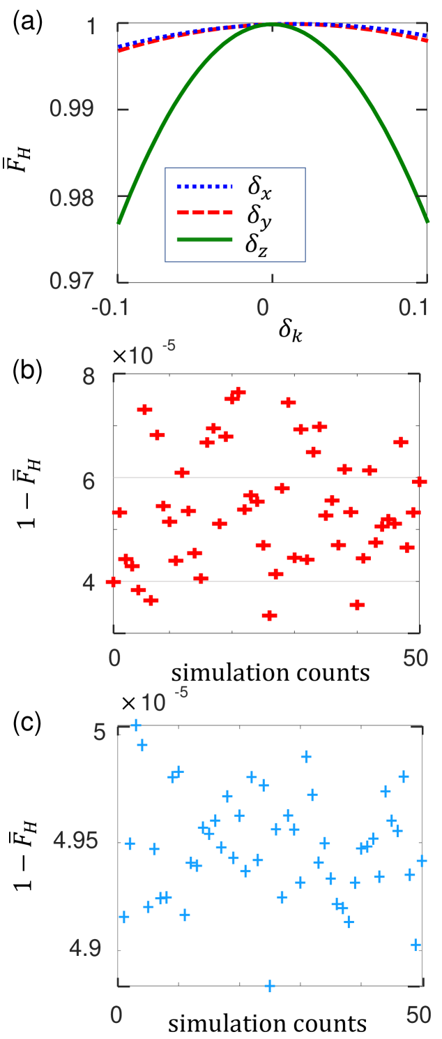
Figure 5: (a) Final-state average fidelities $\bar{F}_{\mathrm{H}}(T)$ versus the systematic error coefficient $\delta_{k}$. (b) Final-state average infidelities, $1-\bar{F}_{\mathrm{H}}(T)$, versus simulation counts with the additive white Gaussian noise (signal-to-noise ratio $R_{\rm{SN}}=10$). (c) Final-state average infidelities, $1-\bar{F}_{\mathrm{H}}(T)$, versus simulation counts with $1/f$ noise (signal-to-noise ratio $\tilde{R}_{\rm{SN}}=10$). We set here: $K=2\pi\times 12.5$ MHz and $\alpha=0.5$.

III.2.1 Example of a two-qubit entangling gate

As an example of the application of a two-qubit entangling gate, we show the implementation of a modified controlled-NOT (CNOT) gate defined by the operator

$$U_{\rm{CNOT}}=\mathbbm{1}_{1}\otimes|\mathcal{C}_{+}\rangle_{2}\langle\mathcal{C}_{+}|+i\sigma_{x}\otimes|\mathcal{C}_{-}\rangle_{2}\langle\mathcal{C}_{-}|,$$ (62)

corresponding to the parameters $\eta_{0}=\pi/2$, $\mu_{0}=\pi/2$, and $\theta=\pi/2$ for $U_{1}$. The following discussion is based on the parameters $\alpha_{1}=\alpha_{2}=0.5$, $K=2\pi\times 12.5$ MHz ($E_{\mathrm{gap}}=161$ MHz), and $T=1~{}\mu$s. The average fidelity $\bar{F}_{\mathrm{CNOT}}(t)$ of the implementation of this CNOT gate over all possible initial states in the computational subspace $\mathcal{S}_{2}$ is defined by [85, 86]

$$\bar{F}_{\mathrm{CNOT}}(t)=\frac{1}{\mathcal{D}_{2}(\mathcal{D}_{2}+1)}\{\mathrm{Tr}[M_{2}(t)M_{2}^{\dagger}(t)]+|\mathrm{Tr}[M_{2}(t)]|^{2}\},$$

where

$$M_{2}(t)=\mathcal{P}_{c2}U^{\dagger}_{\mathrm{CNOT}}U(t)\mathcal{P}_{c2},$$ (63)

given via the projector $\mathcal{P}_{c2}$ and the dimension $\mathcal{D}_{2}=4$ of the computational subspace $\mathcal{S}_{2}$. We plot the time variation of $\bar{F}_{\mathrm{CNOT}}(t)$ in Fig. 4(a), and obtain $\bar{F}_{\mathrm{CNOT}}(T)=0.9997$. Consequently, the modified CNOT gate can be realized almost perfectly.

Populations of different output states with different input states in the implementation of our CNOT-like gate are plotted in Fig. 4(b). As seen, the system does not evolve when the cavity mode 1 is in the cat state $|\mathcal{C}_{+}\rangle_{1}$. However, if the cavity mode 1 is in the cat state $|\mathcal{C}_{-}\rangle_{1}$, a nearly perfect population inversion occurs to the cavity mode 2. The result of Fig. 4(b) also indicates that the CNOT gate is successfully implemented with an extremely small leakage to unwanted levels.

IV Discussions on experimental imperfections

Here, we estimate the performance of the protocol in the presence of different experimental imperfections. We consider our implementation of a Hadamard gate as an example. First, due to an imperfect calibration of the instruments, there may exist systematic errors in the control parameters. The control parameter under the influence of systematic errors can be written as $\Omega_{k}^{e}(t)=(1+\delta_{k})\Omega_{k}(t)$, where $\Omega_{k}^{e}(t)$ is a faulty control parameter and $\delta_{k}$ is the corresponding error coefficient.

We plot the average fidelity $\bar{F}_{\mathrm{H}}$ of the Hadamard gate versus the systematic error coefficient $\delta_{k}$ in Fig. 5(a). It is seen that, when $\delta_{x}\in[-10\%,10\%]$ ($\delta_{y}\in[-10\%,10\%]$), the average fidelity $\bar{F}_{\mathrm{H}}$ remains higher than 0.9969 (0.9973). In addition, the influence on $\bar{F}_{\mathrm{H}}$ caused by systematic errors of $\Omega_{z}(t)$, is larger than those of $\Omega_{x}(t)$ and $\Omega_{y}(t)$, but we can still obtain $\bar{F}_{\mathrm{H}}\geq 0.9768$ when $\delta_{z}\in[-10\%,10\%]$. Therefore, the implementation of the Hadamard gate is robust against systematic errors.

Apart from systematic errors, due to random noise, there are also fluctuations of parameters that may disturb the evolution of the system. Additive white Gaussian noise (AWGN) is a good model to investigate random processes [88, 89, 90, 82]. Therefore, we add AWGN to the control parameter as

$$\Omega_{k}^{n}(t)=\Omega_{k}(t)+\mathrm{AWGN}[\Omega_{k}(t),R_{SN}].$$ (64)

Here, $\mathrm{AWGN}[\Omega_{k}(t),R_{SN}]$ is a function that generates AWGN for the original signal $\Omega_{k}(t)$ with a signal-to-noise ratio $R_{\rm{SN}}$. As AWGN is generated randomly in each single simulation, we perform the numerical simulation averaged over 50 samples to estimate its average effect. Then, $1-\bar{F}_{\mathrm{H}}$ in each single simulation is plotted in Fig. 5(b). Thus, we find the values of the infidelity $1-\bar{F}_{\mathrm{H}}\in[3\times 10^{-5},8\times 10^{-5}]$ averaged over the fifty simulations. The results indicate that the implementation of the Hadamard gate is insensitive to AWGN.

Apart from AWGN, the $1/f$ noise in coherent drives is also a noise limiting the performance of quantum devices. When considering this noise, the control parameter becomes

$$\tilde{\Omega}_{k}^{n}(t)=\Omega_{k}(t)+\mathrm{noise}_{f^{-1}}[\Omega_{k}(t),\tilde{R}_{SN}],$$ (65)

with $\mathrm{noise}_{f^{-1}}[\Omega_{k}(t),\tilde{R}_{SN}]$ being a function generating the $1/f$ noise for the original signal $\Omega_{k}(t)$ with a signal-to-noise ratio $\tilde{R}_{\rm{SN}}$. Here, we also perform numerical simulations averaged over 50 samples to estimate the average effect of the $1/f$ noise with $\tilde{R}_{\rm{SN}}=10$. The results are shown in Fig. 5(c), where we find $1-\bar{F}_{\mathrm{H}}\in[4.884\times 10^{-5},5.004\times 10^{-5}]$ averaged over the fifty simulations. Therefore, our implementation of the Hadamard gate is also insensitive to $1/f$ noise.

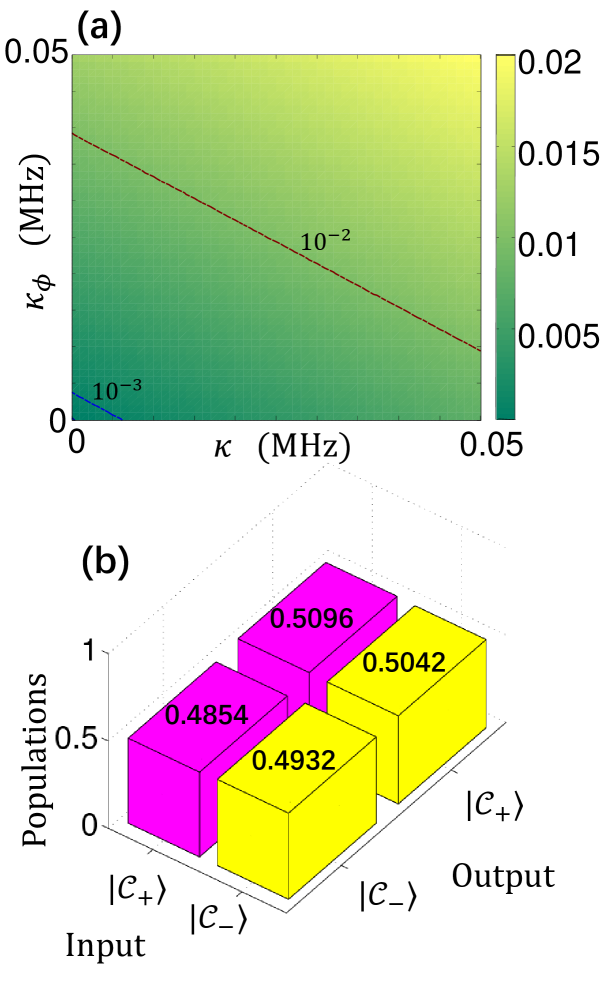
Figure 6: (a) Infidelity $1-F_{\mathrm{H}}$ versus the single photon loss rate $\kappa$ and the dephasing rate $\kappa_{\phi}$ with parameters $K=2\pi\times 12.5$ MHz and $\alpha=0.5$. (b) Populations of different output states for different input states in the implementation of the Hadamard gate ($\kappa=\kappa_{\phi}=0.05$ MHz) with parameters $K=2\pi\times 12.5$ MHz and $\alpha=0.5$.

As the system cannot be completely isolated from the environment in experiments, the interactions between the system and the environment may result in decoherence. We consider two types of decoherence factors, i.e., a single-photon loss and dephasing. The evolution of the system is described by the Lindblad master equation [47]

$$\dot{\rho}(t)= -i[H_{\mathrm{cat}}+H_{\mathrm{add}}(t),\rho(t)]$$ (66)

$$+\frac{\kappa}{2}\mathcal{L}[a]\rho(t)+\frac{\kappa_{\phi}}{2}\mathcal{L}[a^{\dagger}a]\rho(t),$$ (67)

where $\kappa$ ($\kappa_{\phi}$) is the single-photon-loss (dephasing) rate and the Lindblad superoperator $\mathcal{L}$ acting on an arbitrary operator $o$ produces $\mathcal{L}[o]\rho(t)=2o\rho(t)o^{\dagger}-o^{\dagger}o\rho(t)-\rho(t)o^{\dagger}o$. In the presence of decoherence, the evolution is no longer unitary. For the convenience of our discussion, we take the evolution with initial state $|\mathcal{C}_{+}\rangle_{1}$ as an example and analyze the fidelities of the Hadamard gate as

$$F_{\mathrm{H}}={}_{1}\langle\mathcal{C}_{+}|U_{\mathrm{H}}^{\dagger}\rho(T)U_{\mathrm{H}}|\mathcal{C}_{+}\rangle_{1}.$$ (68)

We plot the infidelity $1-F_{\mathrm{H}}$ versus the single photon loss rate $\kappa$ and the dephasing rate $\kappa_{\phi}$ in Fig. 6(a) in the range [0,0.05 MHz] [48]. The results show that the influence of single-photon loss is stronger than dephasing. When $\kappa,\kappa_{\phi}\leq 0.05$ MHz, $1-F_{\mathrm{H}}(T)$ is lower than 0.0201. Therefore, the protocol is robust against single-photon loss and dephasing. In addition, the populations of the output states corresponding to different input states in the implementation of the Hadamard gate with decoherence rates $\kappa=\kappa_{\phi}=0.05$ MHz are plotted in Fig. 6(b). Compared with the results shown in Fig. 3(a), in the presence of decoherence, there exist more faulty populations of the output states. This is because the single-photon loss continuously causes quantum jumps between the cat states $|\mathcal{C}_{\pm}\rangle_{1}$ [49]. The total populations in the subspace $\mathcal{S}$ with the input states $|\mathcal{C}_{\pm}\rangle_{1}$ are both higher than 0.995, showing that the leakage to the unwanted levels outside the subspace $\mathcal{S}$ is still very small in the presence of decoherence.

V Amplification of the cat-state amplitude by squeezing the drive signal

To increase the distinguishability of cat-state qubits, we can introduce a method to amplify the photon numbers inspired by Refs. [78, 79]. When we consider a squeezing operator as $S=\exp[r(a^{{\dagger}2}-a^{2})/2]$, the cat states $\{|\mathcal{C}_{\pm}\rangle\}$ become the amplified cat states $\{|\tilde{\mathcal{C}}_{\pm}\rangle\}$ with $|\tilde{\mathcal{C}}_{\pm}\rangle=S|\mathcal{C}_{\pm}\rangle$ (i.e., squeezed cat states). Here, we omit the subscript “1” for simplicity. The squeezing operator $S$ can be realized by two-photon (squeezing) driving

$$H_{s}=-i\epsilon_{2}(a^{2}-a^{{\dagger}2}),$$ (69)

for the interaction time $t_{s}=r/2\epsilon_{2}$, i.e., switching off the Kerr interaction and the control field [$H_{c}(t)$]. In addition, the inverse transform $\bar{S}=S^{\dagger}$ can be realized by squeezing the driving interaction

$$\bar{H}_{s}=-H_{s}=i\epsilon_{2}(a^{2}-a^{{\dagger}2}),$$ (70)

for the interaction time $t_{s}=r/2\epsilon_{2}$. In this case, the total process can be divided into three steps as shown in Fig. 7.

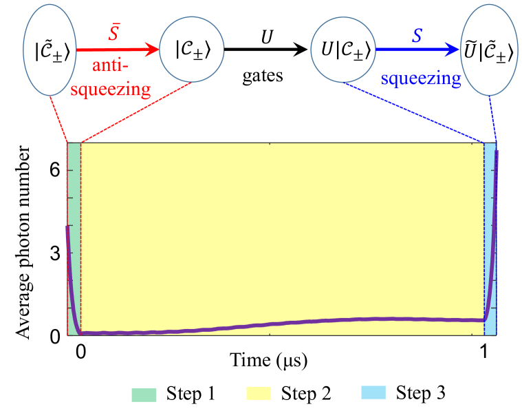
Figure 7: Top panel: The process of NGQC for the amplified cat-state qubits. Bottom panel: Time variation of the average photon number $n_{p}(t)=\mathrm{Tr}[\rho(t)a^{\dagger}a]$. Step 1 (3) is an anti-squeezing (squeezing) process for a measurable input (output) state. Step 2 denotes evolution of the system implementing a given gate (e.g., a Hadamard gate in the bottom panel).

In step 1, we apply the transform $\bar{S}$ to the input state, which is a superposition of the squeezed cat states. In this way, the amplified cat states $\{|\tilde{\mathcal{C}}_{\pm}\rangle\}$ are transformed into small-amplitude cat states $\{|\mathcal{C}_{\pm}\rangle\}$. The step 2 is the geometric gate operation, as illustrated in Sec. III. In step 3, we apply the squeezing transform $S$ to enhance the photon number of the output state, so that the output state can be experimentally detected. The total operator acting on the amplified cat-state qubit is $\tilde{U}=SUS^{\dagger}$, which has the same matrix elements for a small-amplitude cat-state qubit, i.e., $\langle\tilde{\mathcal{C}}_{\jmath}|\tilde{U}|\tilde{\mathcal{C}}_{\jmath^{\prime}}\rangle=\langle\mathcal{C}_{\jmath}|U|\mathcal{C}_{\jmath^{\prime}}\rangle$ ($\jmath,\jmath^{\prime}=\pm$). Here, we assume $r=1.2$ and $\alpha=0.5$, as an example to show the implementation of NGQC for the amplified-cat-state qubits.

We plot the time variation of the average photon number $n_{p}(t)=\mathrm{Tr}[\rho(t)a^{\dagger}a]$ in the bottom panel of Fig. 7. As shown, the average photon number decreases during the first step, corresponding to the anti-squeezing process $|\tilde{\mathcal{C}}_{+}\rangle\rightarrow|\mathcal{C}_{+}\rangle$. Then, by implementing the Hadamard gate, the cat state $|\mathcal{C}_{+}\rangle_{1}$ is transformed into $(|\mathcal{C}_{+}\rangle+|\mathcal{C}_{-}\rangle)/\sqrt{2}$. Finally, in step 3, we amplify the output state by squeezing, i.e.,

$$\frac{1}{\sqrt{2}}\left(|\mathcal{C}_{+}\rangle+|\mathcal{C}_{-}\rangle\right)\rightarrow\frac{1}{\sqrt{2}}\left(|\tilde{\mathcal{C}}_{+}\rangle+|\tilde{\mathcal{C}}_{-}\rangle\right).$$ (71)

The final average photon number is 6.732. The anti-squeezing and squeezing processes are fast (see Fig. 7), so that decoherence in these two processes affects weakly the target state. By considering the experimentally feasible parameters: $\epsilon_{2}=K\alpha^{2}=2\pi\times 3.125$ MHz, $t_{s}=r/\epsilon_{2}=30.56$ ns, and $\kappa=\kappa_{\phi}=0.05$ MHz, we achieve the fidelity $F_{\mathrm{H}}=0.9513$ of the output state $(|\tilde{\mathcal{C}}_{+}\rangle+|\tilde{\mathcal{C}}_{-}\rangle)/\sqrt{2}$ for the Hadamard gate with the initial state $|\tilde{\mathcal{C}}_{+}\rangle$ for the amplified cat-state qubit.

VI Possible implementation using superconducting quantum circuits

VI.1 Single-qubit geometric quantum gates

As shown in Fig. 8, we consider an array-type resonator composed of $N$ superconducting quantum interference devices (SQUIDs) [91, 92, 93, 94, 95, 96, 97]. An ac gate voltage $\tilde{V}_{p}=V_{p}\cos(\omega_{p}t+\varphi_{p})$ (with amplitude $V_{p}$, frequency $\omega_{p}$, and phase $\varphi_{p}$) is applied to induce linear transitions between eigenlevels. The Hamiltonian of this setup reads [93, 95, 97]

$$H_{0}=4E_{C}{\hat{n}}^{2}-NE_{J}[\Phi(t)]\cos\left(\frac{\hat{\phi}}{N}\right)-\frac{E_{C}C_{p}\tilde{V}_{p}}{e}\hat{n},\ \$$ (72)

where $\hat{n}$ is the number of Cooper pairs and $\hat{\phi}$ is the overall phase across the junction array. Here, $E_{C}$ is the resonator charging energy, $E_{J}$ is the Josephson energy of a single SQUID, and $N$ is the number of SQUIDs in the array. The Josephson energy is periodically modulated (with frequency $\omega_{2p}$ and phase $\varphi_{2p}$) by the external magnetic flux $\Phi(t)$, leading to

$$E_{J}[\Phi(t)]=E_{J}+\tilde{E}_{J}\cos(\omega_{2p}t+\varphi_{2p}).$$ (73)

Figure 8: uperconducting quantum circuit for implementing Hamiltonian in Eq. (9). The circuit consists of a SQUID array (black), a shunting capacitor (black), a flux bias line (purple), and an ac gate voltage (red). Here, $\Phi(t)$ is the externally applied magnetic flux, $C_{J}$ is the capacitor shunting the SQUID array, $E_{J}$ is the Josephson energy of a single SQUID, $V_{p}$ is the amplitude of the ac gate voltage, and $C_{p}$ is the gate capacitor.

After the Taylor expansion of $\cos(\hat{\phi}/N)$ to fourth order, we obtain

$$H_{0}\approx ~{}4E_{C}\hat{n}^{2}-NE_{J}(1-\hat{X}+\hat{X}^{2}/6)$$ (74)

$$-N\tilde{E}_{J}(1-\hat{X})\cos(\omega_{2p}t+\varphi_{2p})$$ (75)

$$-\frac{E_{C}C_{p}\tilde{V}_{p}}{e}\hat{n},$$ (76)

where $\hat{X}=(\hat{\phi}/N)^{2}/2$. The quadratic time-independent part of the Hamiltonian can be diagonalized by defining

$$\hat{n}=-in_{0}(a-a^{{\dagger}}),\ \ \hat{\phi}=\phi_{0}(a+a^{{\dagger}}),$$ (77)

where $n_{0}=[E_{J}/(32NE_{C})]^{1/4}$ and ${\phi_{0}}=1/2n_{0}$ are the zero-point fluctuations.

By dropping the constant terms, the Hamiltonian $H_{0}$ becomes

$$H_{0}= ~{}\omega_{c}a^{{\dagger}}a-\frac{E_{C}}{12N^{2}}\left(a+a^{{\dagger}}\right)^{4}$$ (78)

$$+\frac{\tilde{E}_{J}\omega_{c}}{4E_{J}}\left(a+a^{{\dagger}}\right)^{2}\cos(\omega_{2p}t+\varphi_{2p})$$ (79)

$$+i\frac{E_{C}C_{p}{V}_{p}}{e}(a-a^{{\dagger}})\cos(\omega_{p}t+\varphi_{p}),$$ (80)

where $\omega_{c}=\sqrt{8E_{C}E_{J}/N}$. For simplicity, we assume $\omega_{2p}=2\omega_{p}$ and $\varphi_{2p}=-2\xi$. Then, moving into a rotating frame at frequency $\omega_{p}$ and neglecting all of the fast oscillating terms, the approximate Hamiltonian under the rotating wave approximation (RWA) can be written as

$$H_{0}= -Ka^{{\dagger}2}a^{2}+\epsilon_{2}\left(e^{2i\xi}a^{{\dagger}2}+e^{-2i\xi}a^{2}\right)$$ (81)

$$+\chi(t)a^{{\dagger}}a+\epsilon(t)a^{{\dagger}}+\epsilon^{*}(t)a,$$ (82)

where $K=E_{C}/2N^{2}$, $\epsilon_{2}=\omega_{c}\tilde{E}_{J}/8E_{J}$, $\chi(t)=\omega_{c}-\omega_{p}$, and

$$\epsilon(t)=-i\frac{E_{C}C_{p}{V}_{p}}{2e}\exp(-i\varphi_{p}).$$ (83)

Then, by defining $a_{1}\equiv a$, we recover the total Hamiltonian $H_{\rm{tot}}(t)$ given in Eq. (9) for the single-qubit case. Note that, as shown in [98], the Kerr nonlinearity (which is a rescaled third-order susceptibility of a nonlinear medium) can be exponentially enhanced by applying quadrature squeezing, which interaction with a medium is proportional to its second-order susceptibility. This means that one can exponentially amplify higher-order nonlinearities by applying lower-order nonlinear effects. Other methods of applying quadrature squeezing to increase nonlinear interactions are described in, e.g., [99, 100, 101].

VI.2 Errors in the sperconducting circuit

According to the above analysis, the control drives depend on the parameters $E_{C}$, $E_{J}$, and $V_{p}$. Assuming that the parameters with errors respectively become

$$E_{C}\rightarrow E_{C}+\delta\!E_{C},\ E_{J}\rightarrow E_{J}+\delta\!E_{J},\ V_{p}\rightarrow V_{p}+\delta\!V_{p}.$$

The errors in the control parameters can be approximately calculated by

$$\delta\!\omega_{c}\simeq\frac{\omega_{c}}{2}(\frac{\delta\!E_{J}}{E_{J}}+\frac{\delta\!E_{C}}{E_{C}}),\ \delta\!K=\frac{K\delta\!E_{C}}{E_{C}},$$

(84)

$$\delta\!\epsilon_{2}\simeq\frac{\epsilon_{2}}{2}\left(\frac{\delta\!E_{C}}{E_{C}}-\frac{\delta\!E_{J}}{E_{J}}\right),$$ (85)

(86)

$$\delta\!\epsilon(t)\simeq\left(\frac{\delta\!E_{C}}{E_{C}}+\frac{\delta\!V_{p}}{V_{p}}\right)\epsilon(t).$$ (87)

Therefore, when considering the errors in the control parameters, the Hamiltonian becomes

$$H_{0}^{\prime}= H_{0}+\delta\!H_{\rm{cat}}+\delta\!H_{c},$$ (88)

$$\delta\!H_{\rm{cat}}= -\delta\!Ka^{{\dagger}2}a^{2}+\delta\!\epsilon_{2}\left(e^{2i\xi}a^{{\dagger}2}+e^{-2i\xi}a^{2}\right),$$ (89)

$$\delta\!H_{c}= \delta\!\omega_{c}a^{{\dagger}}a+\delta\!\epsilon(t)a^{{\dagger}}+\delta\!\epsilon^{*}(t)a,$$ (90)

where $\delta\!H_{\rm{cat}}$ induces an error on the amplitude of the coherence states $|\!\pm\alpha\rangle$ as

$$\delta\!\alpha\simeq-\frac{\alpha}{4}\left(\frac{2\delta\!E_{C}}{E_{C}}-\frac{\delta\!E_{J}}{E_{J}}\right),$$ (91)

and $\delta\!H_{c}$ influences the control drives designed by invariant-based reverse engineering.

For $|\delta\!E_{C}/E_{C}|,|\delta\!E_{J}/E_{J}|\leq 0.1$, and $\alpha=0.5$, the absolute error of the coherent-state amplitude approximately satisfies $|\delta\!\alpha|\leq 0.0375$. Because of

$$1-|\langle\tilde{\alpha}_{+}|\alpha\rangle|^{2}\simeq 1-|\langle\tilde{\alpha}_{-}|\alpha\rangle|^{2}\simeq 0.001,$$ (92)

with $\tilde{\alpha}_{\pm}=0.5\pm 0.0375$, the cat qubit can be near perfectly stabilized in the preset states by a small fluctuation of the amplitude $\alpha$.

Moreover, according to Eq. (16) and $\delta\!H_{c}$ in Eq. (88), the errors in $\Omega_{x}(t)$, $\Omega_{y}(t)$, and $\Omega_{z}(t)$ can be approximately described by the linear superpositions of $\delta\!E_{J}$, $\delta\!E_{C}$, and $\delta\!V_{p}$. Therefore, when $E_{J}$, $E_{C}$, and $V_{p}$ are subjected to AWGN or $1/f$ noise, the wave shapes of $\Omega_{x}(t)$, $\Omega_{y}(t)$, and $\Omega_{z}(t)$ are also mixed with the same type of noise. According to the analysis in Sec. IV, the fidelities of the gates are insensitive to these types of noise in $\Omega_{x}(t)$, $\Omega_{y}(t)$, and $\Omega_{z}(t)$. Consequently, our proposal is robust against AWGN and $1/f$ noise in $E_{J}$ and $E_{C}$ of the considered superconducting circuits.

VI.3 Kitten states

We also note that the Kerr nonlinearity enables the generation of not only conventional (i.e., two-component) Schrödinger cat states, i.e., superpositions of two macroscopically distinct states, but also the generation of superpositions of a larger number of macroscopically distinct states. The states are referred to as Schrödinger kitten states or multi-component cat-like states, as predicted in [102] and experimentally generated via the Kerr interaction in superconducting quantum circuits in [103]. These kitten states, which are examples of Gauss sums, have been used in an unconventional algorithm for number factorization, i.e., to distinguish between factors and nonfactors. Implementations of the Gauss-sums algorithm include NMR spectroscopy [104, 105] and Ramsey spectroscopy using cold atoms [106].

VI.4 Two-qubit geometric entangling gates

To realize two-qubit geometric gates, we consider two superconducting circuits with the same structure shown in Fig. 8. The two circuits are coupled with each other through a Josephson-junction coupler with Josephson energy $\bar{E}_{J}$ [107, 87]. The coupler provides a coupling between the two circuits as

$$\mathcal{U}_{J}=-\bar{E}_{J}\cos\left[\hat{\phi}_{2}-\hat{\phi}_{1}+2\pi\frac{\bar{\Phi}(t)}{\Phi_{0}}\right],$$ (93)

with $\hat{\phi}_{m}=\phi_{0m}(a_{m}+a^{{\dagger}}_{m})$ ($m=1,2$). Here, $\bar{\Phi}(t)$ is the external flux applied to the loop of the coupler, and $\Phi_{0}$ is the flux quantum. By modulating $\bar{\Phi}(t)$ at the frequency of the second circuit, the required cross-Kerr nonlinearity $\chi_{ab}(t)a^{\dagger}_{1}a_{1}a^{\dagger}_{2}a_{2}$ and the longitudinal interaction $a^{\dagger}_{1}a_{1}[\lambda^{*}_{1}(t)a_{2}+\lambda_{1}(t)a^{\dagger}_{2}]$ can be realized with the Taylor expansion of $\cos[\hat{\phi}_{2}-\hat{\phi}_{1}+2\pi\bar{\Phi}(t)/\Phi_{0}]$ to fourth order [87]. The coupling between two circuits changes the detuning and strength of the two-photon drive of each circuit. However, to diagonalize the quadratic time-independent part of the Hamiltonian, the coefficients of $\hat{n}_{m}^{2}$ and $\hat{\phi}_{m}^{2}$ should be set equal, where $\hat{n}_{m}=-in_{0m}(a_{m}-a^{{\dagger}}_{m})$. Consequently, one can derive that the strength of the self-Kerr nonlinearity for each circuit is still expressed by $K=E_{C}/2N^{2}$.

VI.5 Comparison of gate times

We now compare the gate time of our proposal with previous experiments. Relevant information is also listed in Table 2.

The gate time in our proposal is comparable with that in previous experiments using superconducting systems. For example, the gate time of a controlled-$\pi$-phase gate in Ref. [108] using superconducting qubits is about 113 ns, with gate fidelities $\sim 0.99$. In Ref. [109], the gate time for implementing the Hadamard gate and the NOT gate with fidelities $\sim 0.99$ (by using a transmon qubit coupled to a transmission-line resonator) is $\sim 62.5$ ns. In our proposal, to implement the NOT and Hadamard gates with fidelity higher than 0.99, the gate time can be selected as $T=210$ ns. To implement the CNOT gate with fidelity higher than 0.99, the gate time in the present scheme is about 220 ns.

Moreover, compared with some previous methods using dipole interactions between neutral atoms, the gate time for two-qubit gates in the present approach is generally shorter. For example, in Ref. [90], the gate time to realize the controlled-$\pi$-phase gate with about $10^{-4}$ infidelity is 376.16 $\mu$s using the available dipole interaction strengths $V=20$ MHz. In the scheme of Ref. [40], the gate time to implement the CNOT gate for two neutral atoms with infidelity about $10^{-3}$ is 85.94 $\mu$s, using the reported dipole interaction strengths $V=2\pi\times 50$ MHz.

In the present protocol, the gate times for implementing the controlled-$\pi$-phase gate and the CNOT gate, with infidelities about $10^{-4}$ to $10^{-3}$, can be both less than 1 $\mu$s with the available Kerr nonlinearity $K=2\pi\times 12.5$ MHz. The longer gate times of the controlled-$\pi$-phase gate and the CNOT gate in the schemes of Refs. [90, 40] is because these protocols should work in the Rydberg blockade regime, which limits the strength of the control fields.

Recently, some modified nonadiabatic geometric quantum computation methods [110, 111, 112, 113], based on the dipole interactions of neutral atoms, have been proposed, which work in different regimes and relax the limitation of strong amplitudes of control fields. The gate times of the controlled-$\pi$-phase gate and the CNOT gate in these schemes can be improved to about 1–10 $\mu$s. In the present protocol, as the Kerr nonlinearity can provide much bounder energy gap between eigenvectors of $H_{\mathrm{cat}}$, the control fields with stronger amplitudes can be adopted.

In addition, as reported in the scheme of Ref. [114], to implement multi-atom geometric quantum gates in cavity quantum electrodynamics system with the amplitude of laser pulses about 50-200 MHz with fidelity over 0.999, the gate time is about 0.5–3 $\mu$s, which is also close to the gate time in the present approach.

Compared with the present method, the gate time of the nonadiabatic geometric quantum computation schemes [115, 116] in trapped-ion systems is slower. Because these schemes work in the Lamb-Dicke limit, the amplitudes of driving pulses should be much less than the frequency (1–10 MHz) of the vibration modes of trapped ions, and the gate time is about 1–2 ms.

Table 2: Comparison of the gate times between previously reported schemes and ours

Year	Reference	System	Gate	Gate time	Fidelity
2014	Ref. [115]	Trapped ions	Hadamard, Phase	$\sim$1–2 ms	$\gtrsim 0.99$
2017	Ref. [109]	Superconducting circuits	NOT, Hadamard	$\sim 62.5$ ns	$\gtrsim 0.99$
2018	Ref. [90]	Rydberg atoms	Controlled-$\pi$-phase	$\sim 376.16$ $\mu$s	$\gtrsim 0.999$
2018	Ref. [114]	Cavity QED	Controlled-$\pi$-phase, Toffoli	$\sim$0.5–3 $\mu$s	$\gtrsim 0.999$
2019	Ref. [116]	Trapped ions	CNOT	$\sim$1–2 ms	$\gtrsim 0.99$
2020	Ref. [108]	Superconducting circuits	Controlled-$\pi$-phase	$\sim 113$ ns	$\gtrsim 0.99$
2020	Ref. [40]	Rydberg atoms	CNOT	$\sim 85.94$ $\mu$s	$\gtrsim 0.999$
2020	Ref. [110]	Rydberg atoms	Controlled-$\pi$-phase, CNOT	$\sim 8$ $\mu$s	$\gtrsim 0.99$
2021	Ref. [111]	Rydberg atoms	SWAP	$\sim 7.7$ $\mu$s	$\gtrsim 0.99$
2021	Ref. [113]	Rydberg atoms	CNOT	$\sim 1$ $\mu$s	$\gtrsim 0.99$
Our proposal		Superconducting circuits	NOT, Phase, Hadamard, CNOT	$\sim$210–220 ns	$\gtrsim 0.99$

VII Conclusion

In conclusion, we have proposed a method to realize nonadiabatic geometric quantum computation using cat qubits with invariant-based reverse engineering. The evolution of the cavity mode is restricted to a subspace spanned by a pair of Schrödinger cat states assisted by a Kerr nonlinearity and a two-photon squeezing drive, so that one can generate photonic cat qubits. We add a coherent field to linearly drive the cavity mode, inducing oscillations between dressed cat states. When designing the control fields by invariant-based reverse engineering, the system can evolve quasiperiodically and acquire only pure geometric phases. Thus, one can realize nonadiabatic geometric quantum computation with a cat qubit. By amplifying the amplitudes of different cat states, the input and output states can be easily detected in experiments.

Two-qubit quantum gates for cat qubits are also considered with couplings between two cavity modes. As we have shown, the controlled two-qubit geometric quantum entangling gates can also be implemented with high fidelities. The influence of systematic errors, AWGN, $1/f$ noise, and decoherence (including photon loss and dephasing), was studied here using numerical simulations. The results indicate that our approach is robust against these errors. Therefore, our protocol can provide efficient high-fidelity quantum gates for nonadiabatic geometric quantum computation in bosonic systems.

Appendix A Derivation of a dynamic invariant and the choice of parameters for eliminating dynamical phases

Because the Hamiltonian $H_{c}(t)=\vec{\Omega}(t)\cdot\vec{\sigma}$ possesses SU(2) dynamic structure, there is a dynamic invariant $I(t)$ in form of $I(t)=\vec{\zeta}(t)\cdot\vec{\sigma}$ [117, 82]. The commutative relation of $H_{c}(t)$ and $I(t)$ can be calculated as

$$[H_{c}(t),I(t)] = ~{}[\vec{\Omega}(t)\cdot\vec{\sigma}][\vec{\zeta}(t)\cdot\vec{\sigma}]-[\vec{\zeta}(t)\cdot\vec{\sigma}][\vec{\Omega}(t)\cdot\vec{\sigma}]$$ (94)

$$= ~{}\{\vec{\sigma}\times[\vec{\Omega}(t)\times\vec{\zeta}(t)]\}\cdot\vec{\sigma}$$ (96)

$$= ~{}(\vec{\sigma}\times\vec{\sigma})\cdot[\vec{\Omega}(t)\times\vec{\zeta}(t)]$$ (98)

$$= ~{}2i[\vec{\Omega}(t)\times\vec{\zeta}(t)]\cdot\vec{\sigma}.$$ (100)

Substituting Eq. (94) into Eq. (1), we obtain $\dot{\vec{\zeta}}(t)=2[\vec{\Omega}(t)\times\vec{\zeta}(t)]$. Moreover,

$$\frac{1}{2}\frac{d}{dt}|\vec{\zeta}(t)|^{2}= ~{}\vec{\zeta}(t)\cdot\dot{\vec{\zeta}}(t)=2\vec{\zeta}(t)\cdot[\vec{\Omega}(t)\times\vec{\zeta}(t)]$$ (101)

$$= ~{}2\vec{\Omega}(t)\cdot[\vec{\zeta}(t)\times\vec{\zeta}(t)]=0,$$ (102)

implies that $|\vec{\zeta}(t)|$ should be constant.

When $|\vec{\zeta}(t)|=1$, one can parametrize $\vec{\zeta}(t)$ as $(\sin{\eta}\sin{\mu},\cos{\eta}\sin{\mu},\cos{\mu})$, and derive the eigenvectors $|\phi_{\pm}(t)\rangle$ of the invariant $I(t)$ as given in Eq. (14). The time derivatives of the dynamical phases $\vartheta_{\pm}(t)$ and the geometric phases $\Theta_{\pm}(t)$ acquired by $|\phi_{\pm}(t)\rangle$ are

$$\dot{\vartheta}_{\pm}(t)=\mp\left[\Omega_{z}(t)+\frac{1}{2}\dot{\eta}\sin^{2}\mu\right]\sec\mu,$$ (103)

$$\dot{\Theta}_{\pm}(t)=\pm\dot{\eta}\sin^{2}\left(\frac{\mu}{2}\right).$$ (104)

To eliminate the dynamical phases, we choose

$$\Omega_{z}(t)=-\frac{1}{2}\dot{\eta}(t)\sin^{2}[\mu(t)].$$ (105)

In addition, by reversely solving $\dot{\vec{\zeta}}(t)=2[\vec{\Omega}(t)\times\vec{\zeta}(t)]$, we obtain

$$\Omega_{x}(t)= ~{}\frac{1}{2}\vec{e}_{z}\cdot[\vec{\nu}_{1}(t)\times\vec{\nu}_{2}(t)],$$ (106)

$$\Omega_{y}(t)= ~{}\frac{1}{2}\vec{\nu}_{1}(t)\cdot\vec{\nu}_{2}(t),$$ (107)

$$\vec{\nu}_{1}(t)= ~{}[2\Omega_{z}(t)+\dot{\eta}(t)]\tan[\mu(t)]\vec{e}_{x}+\dot{\mu}(t)\vec{e}_{y},$$ (108)

$$\vec{\nu}_{2}(t)= ~{}\cos[\eta(t)]\vec{e}_{x}+\sin[\eta(t)]\vec{e}_{y}.$$ (109)

Combining Eqs. (105) and (106), we derive Eq. (16) as shown in Sec. III.

References

- Nielsen and Chuang [2000] M. A. Nielsen and I. L. Chuang, Quantum Computation and Quantum Information (Cambridge University Press, Cambridge, 2000).
- Bennett and DiVincenzo [2000] C. H. Bennett and D. P. DiVincenzo, Quantum information and computation, Nature (London) 404, 247 (2000).
- Gribbin [2014] J. Gribbin, Computing with Quantum Cats: From Colossus to Qubits (Prometheus Books, 2014).
- Zhong et al. [2020] H.-S. Zhong et al., Quantum computational advantage using photons, Science 370, 1460 (2020).
- Duarte and Taylor [2021] F. J. Duarte and T. S. Taylor, Quantum Entanglement Engineering and Applications, 2053-2563 (IOP Publishing, 2021).
- Haroche and Raimond [2000] S. Haroche and J. M. Raimond, Exploring the Quantum: Atoms, Cavities, and Photons (Oxford University Press, Oxford, 2000).
- Arute et al. [2019] F. Arute et al., Quantum supremacy using a programmable superconducting processor, Nature (London) 574, 505 (2019).
- Chen et al. [2021a] Y.-A. Chen et al., An integrated space-to-ground quantum communication network over 4,600 kilometres, Nature (London) 589, 214 (2021a).
- Aasi et al. [2013] J. Aasi et al., Enhanced sensitivity of the LIGO gravitational wave detector by using squeezed states of light, Nat. Photon. 7, 613 (2013).
- Grote et al. [2013] H. Grote, K. Danzmann, K. L. Dooley, R. Schnabel, J. Slutsky, and H. Vahlbruch, First long-term application of squeezed states of light in a gravitational-wave observatory, Phys. Rev. Lett. 110, 181101 (2013).
- Acernese et al. [2019] F. Acernese et al. (Virgo Collaboration), Increasing the astrophysical reach of the advanced virgo detector via the application of squeezed vacuum states of light, Phys. Rev. Lett. 123, 231108 (2019).
- Tse et al. [2019] M. Tse et al., Quantum-enhanced advanced LIGO detectors in the era of gravitational-wave astronomy, Phys. Rev. Lett. 123, 231107 (2019).
- Ekert and Jozsa [1996] A. Ekert and R. Jozsa, Quantum computation and Shor’s factoring algorithm, Rev. Mod. Phys. 68, 733 (1996).
- Grover [1997] L. K. Grover, Quantum mechanics helps in searching for a needle in a haystack, Phys. Rev. Lett. 79, 325 (1997).
- Cen et al. [2006] L.-X. Cen, Z. D. Wang, and S. J. Wang, Scalable quantum computation in decoherence-free subspaces with trapped ions, Phys. Rev. A 74, 032321 (2006).
- Zhu and Zanardi [2005] S.-L. Zhu and P. Zanardi, Geometric quantum gates that are robust against stochastic control errors, Phys. Rev. A 72, 020301(R) (2005).
- Sjöqvist [2008] E. Sjöqvist, A new phase in quantum computation, Physics 1, 35 (2008).
- Lv et al. [2020] Q.-X. Lv, Z.-T. Liang, H.-Z. Liu, J.-H. Liang, K.-Y. Liao, and Y.-X. Du, Noncyclic geometric quantum computation with shortcut to adiabaticity, Phys. Rev. A 101, 022330 (2020).
- Zanardi and Rasetti [1999] P. Zanardi and M. Rasetti, Holonomic quantum computation, Phys. Lett. A 264, 94 (1999).
- Duan et al. [2001] L.-M. Duan, J. I. Cirac, and P. Zoller, Geometric manipulation of trapped ions for quantum computation, Science 292, 1695 (2001).
- Wu et al. [2005] L.-A. Wu, P. Zanardi, and D. A. Lidar, Holonomic quantum computation in decoherence-free subspaces, Phys. Rev. Lett. 95, 130501 (2005).
- Ashhab et al. [2006] S. Ashhab, J. R. Johansson, and F. Nori, Decoherence in a scalable adiabatic quantum computer, Phys. Rev. A 74, 052330 (2006).
- Ashhab and Nori [2010] S. Ashhab and F. Nori, Control-free control: Manipulating a quantum system using only a limited set of measurements, Phys. Rev. A 82, 062103 (2010).
- Zheng et al. [2010] S.-B. Zheng, C.-P. Yang, and F. Nori, Arbitrary control of coherent dynamics for distant qubits in a quantum network, Phys. Rev. A 82, 042327 (2010).
- Wilson et al. [2012] R. D. Wilson, A. M. Zagoskin, S. Savel’ev, M. J. Everitt, and F. Nori, Feedback-controlled adiabatic quantum computation, Phys. Rev. A 86, 052306 (2012).
- Zhang et al. [2017] J. Zhang, Y.-X. Liu, R.-B. Wu, K. Jacobs, and F. Nori, Quantum feedback: Theory, experiments, and applications, Physics Reports 679, 1 (2017).
- Zhu and Wang [2002] S.-L. Zhu and Z. D. Wang, Implementation of universal quantum gates based on nonadiabatic geometric phases, Phys. Rev. Lett. 89, 097902 (2002).
- Sjöqvist et al. [2012] E. Sjöqvist, D. M. Tong, L. M. Andersson, B. Hessmo, M. Johansson, and K. Singh, Non-adiabatic holonomic quantum computation, New J. Phys. 14, 103035 (2012).
- Xu et al. [2012] G. F. Xu, J. Zhang, D. M. Tong, E. Sjöqvist, and L. C. Kwek, Nonadiabatic holonomic quantum computation in decoherence-free subspaces, Phys. Rev. Lett. 109, 170501 (2012).
- Martínez-Garaot et al. [2014] S. Martínez-Garaot, E. Torrontegui, X. Chen, and J. G. Muga, Shortcuts to adiabaticity in three-level systems using Lie transforms, Phys. Rev. A 89, 053408 (2014).
- Li et al. [2018] Y.-C. Li, D. Martínez-Cercós, S. Martínez-Garaot, X. Chen, and J. G. Muga, Hamiltonian design to prepare arbitrary states of four-level systems, Phys. Rev. A 97, 013830 (2018).
- Guéry-Odelin et al. [2019] D. Guéry-Odelin, A. Ruschhaupt, A. Kiely, E. Torrontegui, S. Martínez-Garaot, and J. G. Muga, Shortcuts to adiabaticity: Concepts, methods, and applications, Rev. Mod. Phys. 91, 045001 (2019).
- Kang et al. [2020a] Y.-H. Kang, Z.-C. Shi, Y. Xia, and J. Song, Robust generation of logical qubit singlet states with reverse engineering and optimal control with spin qubits, Adv. Quantum Tech. 3, 2000113 (2020a).
- Wei et al. [2008] L. F. Wei, J. R. Johansson, L. X. Cen, S. Ashhab, and F. Nori, Controllable coherent population transfers in superconducting qubits for quantum computing, Phys. Rev. Lett. 100, 113601 (2008).
- Daems et al. [2013] D. Daems, A. Ruschhaupt, D. Sugny, and S. Guérin, Robust quantum control by a single-shot shaped pulse, Phys. Rev. Lett. 111, 050404 (2013).
- Van-Damme et al. [2017] L. Van-Damme, D. Schraft, G. T. Genov, D. Sugny, T. Halfmann, and S. Guérin, Robust not gate by single-shot-shaped pulses: Demonstration of the efficiency of the pulses in rephasing atomic coherences, Phys. Rev. A 96, 022309 (2017).
- Du et al. [2019] Y.-X. Du, Z.-T. Liang, H. Yan, and S.-L. Zhu, Geometric quantum computation with shortcuts to adiabaticity, Adv. Quantum Tech. 2, 1970051 (2019).
- Xue et al. [2016] Z.-Y. Xue, J. Zhou, Y.-M. Chu, and Y. Hu, Nonadiabatic holonomic quantum computation with all-resonant control, Phys. Rev. A 94, 022331 (2016).
- Xu et al. [2017] G. F. Xu, P. Z. Zhao, T. H. Xing, E. Sjöqvist, and D. M. Tong, Composite nonadiabatic holonomic quantum computation, Phys. Rev. A 95, 032311 (2017).
- Kang et al. [2020b] Y.-H. Kang, Z.-C. Shi, J. Song, and Y. Xia, Heralded atomic nonadiabatic holonomic quantum computation with Rydberg blockade, Phys. Rev. A 102, 022617 (2020b).
- Abdumalikov et al. [2013] A. A. Abdumalikov, J. M. Fink, K. Juliusson, M. Pechal, S. Berger, A. Wallraff, and S. Filipp, Experimental realization of non-Abelian non-adiabatic geometric gates, Nature (London) 496, 482 (2013).
- Zhou et al. [2017] B. B. Zhou, P. C. Jerger, V. O. Shkolnikov, F. J. Heremans, G. Burkard, and D. D. Awschalom, Holonomic quantum control by coherent optical excitation in diamond, Phys. Rev. Lett. 119, 140503 (2017).
- Xu et al. [2018] Y. Xu et al., Single-loop realization of arbitrary nonadiabatic holonomic single-qubit quantum gates in a superconducting circuit, Phys. Rev. Lett. 121, 110501 (2018).
- Hu et al. [2019] L. Hu et al., Quantum error correction and universal gate set operation on a binomial bosonic logical qubit, Nature Physics 15, 503 (2019).
- Ma et al. [2020] Y. Ma et al., Error-transparent operations on a logical qubit protected by quantum error correction, Nature Physics 16, 827 (2020).
- Zhang et al. [2018] J. Zhang, S. J. Devitt, J. Q. You, and F. Nori, Holonomic surface codes for fault-tolerant quantum computation, Phys. Rev. A 97, 022335 (2018).
- Mirrahimi et al. [2014] M. Mirrahimi, Z. Leghtas, V. V. Albert, S. Touzard, R. J. Schoelkopf, L. Jiang, and M. H. Devoret, Dynamically protected cat-qubits: a new paradigm for universal quantum computation, New J. Phys. 16, 045014 (2014).
- Leghtas et al. [2015] Z. Leghtas et al., Confining the state of light to a quantum manifold by engineered two-photon loss, Science 347, 853 (2015).
- Puri et al. [2017] S. Puri, S. Boutin, and A. Blais, Engineering the quantum states of light in a Kerr-nonlinear resonator by two-photon driving, npj Quantum Inf. 3 (2017).
- Guillaud and Mirrahimi [2019] J. Guillaud and M. Mirrahimi, Repetition cat qubits for fault-tolerant quantum computation, Phys. Rev. X 9, 041053 (2019).
- Grimm et al. [2020] A. Grimm, N. E. Frattini, S. Puri, S. O. Mundhada, S. Touzard, M. Mirrahimi, S. M. Girvin, S. Shankar, and M. H. Devoret, Stabilization and operation of a Kerr-cat qubit, Nature (London) 584, 205 (2020).
- Dodonov et al. [1974] V. V. Dodonov, I. A. Malkin, and V. I. Man’ko, Even and odd coherent states and excitations of a singular oscillator, Physica 72, 597 (1974).
- Ralph et al. [2003] T. C. Ralph, A. Gilchrist, G. J. Milburn, W. J. Munro, and S. Glancy, Quantum computation with optical coherent states, Phys. Rev. A 68, 042319 (2003).
- Gilchrist et al. [2004] A. Gilchrist, K. Nemoto, W. J. Munro, T. C. Ralph, S. Glancy, S. L. Braunstein, and G. J. Milburn, Schrödinger cats and their power for quantum information processing, J. Opt. B 6, S828 (2004).
- Liu et al. [2005] Y.-X. Liu, L. F. Wei, and F. Nori, Preparation of macroscopic quantum superposition states of a cavity field via coupling to a superconducting charge qubit, Phys. Rev. A 71, 063820 (2005).
- Kira et al. [2011] M. Kira, S. W. Koch, R. P. Smith, A. E. Hunter, and S. T. Cundiff, Quantum spectroscopy with Schrödinger-cat states, Nat. Phys. 7, 799 (2011).
- Gribbin [2013] J. Gribbin, Computing with Quantum Cats: From Colossus to Qubits (London, Bantam Press, 2013).
- Puri et al. [2019] S. Puri et al., Stabilized cat in a driven nonlinear cavity: A fault-tolerant error syndrome detector, Phys. Rev. X 9, 041009 (2019).
- Chen et al. [2021b] Y.-H. Chen, W. Qin, X. Wang, A. Miranowicz, and F. Nori, Shortcuts to adiabaticity for the quantum Rabi model: Efficient generation of giant entangled cat states via parametric amplification, Phys. Rev. Lett. 126, 023602 (2021b).
- Qin et al. [2021] W. Qin, A. Miranowicz, H. Jing, and F. Nori, Generating long-lived macroscopically distinct superposition states in atomic ensembles, Phys. Rev. Lett. 127, 093602 (2021).
- Gottesman et al. [2001] D. Gottesman, A. Kitaev, and J. Preskill, Encoding a qubit in an oscillator, Phys. Rev. A 64, 012310 (2001).
- Terhal [2015] B. M. Terhal, Quantum error correction for quantum memories, Rev. Mod. Phys. 87, 307 (2015).
- Gaitan [2008] F. Gaitan, Quantum Error Correction and Fault Tolerant Quantum Computing (CRC Press, Boca Raton, 2008).
- Lidar and Brun [2013] D. A. Lidar and T. A. Brun, eds., Quantum Error Correction (Cambridge Univ. Press, New York, 2013).
- Mirrahimi [2016] M. Mirrahimi, Cat-qubits for quantum computation, Comptes Rendus Phys. 17, 778 (2016).
- Albert et al. [2016] V. V. Albert et al., Holonomic quantum control with continuous variable systems, Phys. Rev. Lett. 116, 140502 (2016).
- Michael et al. [2016] M. H. Michael, M. Silveri, R. T. Brierley, V. V. Albert, J. Salmilehto, L. Jiang, and S. M. Girvin, New class of quantum error-correcting codes for a bosonic mode, Phys. Rev. X 6, 031006 (2016).
- Albert et al. [2018] V. V. Albert et al., Performance and structure of single-mode bosonic codes, Phys. Rev. A 97, 032346 (2018).
- Albert et al. [2019] V. V. Albert, S. O. Mundhada, A. Grimm, S. Touzard, M. H. Devoret, and L. Jiang, Pair-cat codes: autonomous error-correction with low-order nonlinearity, Quantum Sci. Tech. 4, 035007 (2019).
- Litinski [2019] D. Litinski, A game of surface codes: Large-scale quantum computing with lattice surgery, Quantum 3, 128 (2019).
- Grimsmo et al. [2020] A. L. Grimsmo, J. Combes, and B. Q. Baragiola, Quantum computing with rotation-symmetric bosonic codes, Phys. Rev. X 10, 011058 (2020).
- Chen et al. [2021c] Y.-H. Chen, W. Qin, R. Stassi, X. Wang, and F. Nori, Fast binomial-code holonomic quantum computation with ultrastrong light-matter coupling, Phys. Rev. Research 3, 033275 (2021c).
- Chamberland et al. [2020a] C. Chamberland et al., Building a fault-tolerant quantum computer using concatenated cat codes, arXiv:2012.04108 (2020a).
- Ma et al. [2021] W.-L. Ma, S. Puri, R. J. Schoelkopf, M. H. Devoret, S. M. Girvin, and L. Jiang, Quantum control of bosonic modes with superconducting circuits, Sci. Bull. 66, 1789 (2021).
- Cai et al. [2021] W. Cai, Y. Ma, W. Wang, C.-L. Zou, and L. Sun, Bosonic quantum error correction codes in superconducting quantum circuits, Fund. Res. 1, 50 (2021).
- Chamberland et al. [2020b] C. Chamberland et al., Building a fault-tolerant quantum computer using concatenated cat codes (2020b), arXiv:2012.04108 [quant-ph] .
- Chen et al. [2021d] Y.-H. Chen, R. Stassi, W. Qin, A. Miranowicz, and F.Nori, Fault-tolerant multi-qubit geometric entangling gates using photonic cat qubits, arXiv:2109.04643 (2021d).
- Sekatski et al. [2009] P. Sekatski, N. Brunner, C. Branciard, N. Gisin, and C. Simon, Towards quantum experiments with human eyes as detectors based on cloning via stimulated emission, Phys. Rev. Lett. 103, 113601 (2009).
- Qin et al. [2019] W. Qin, A. Miranowicz, G. Long, J. Q. You, and F. Nori, Proposal to test quantum wave-particle superposition on massive mechanical resonators, npj Quantum Inf. 5, 58 (2019).
- Lewis and Riesenfeld [1969] H. R. Lewis and W. B. Riesenfeld, An exact quantum theory of the time-dependent harmonic oscillator and of a charged particle in a time-dependent electromagnetic field, J. Math. Phys. 10, 1458 (1969).
- Liu et al. [2019] B.-J. Liu, X.-K. Song, Z.-Y. Xue, X. Wang, and M.-H. Yung, Plug-and-play approach to nonadiabatic geometric quantum gates, Phys. Rev. Lett. 123, 100501 (2019).
- Kang et al. [2020c] Y.-H. Kang, Z.-C. Shi, B.-H. Huang, J. Song, and Y. Xia, Flexible scheme for the implementation of nonadiabatic geometric quantum computation, Phys. Rev. A 101, 032322 (2020c).
- Liang et al. [2016] Z.-T. Liang, X. Yue, Q. Lv, Y.-X. Du, W. Huang, H. Yan, and S.-L. Zhu, Proposal for implementing universal superadiabatic geometric quantum gates in nitrogen-vacancy centers, Phys. Rev. A 93, 040305(R) (2016).
- Ji et al. [2019] L.-N. Ji, T. Chen, and Z.-Y. Xue, Scalable nonadiabatic holonomic quantum computation on a superconducting qubit lattice, Phys. Rev. A 100, 062312 (2019).
- Zanardi and Lidar [2004] P. Zanardi and D. A. Lidar, Purity and state fidelity of quantum channels, Phys. Rev. A 70, 012315 (2004).
- Pedersen et al. [2007] L. H. Pedersen, N. M. Møller, and K. Mølmer, Fidelity of quantum operations, Phys. Lett. A 367, 47 (2007).
- Touzard et al. [2019] S. Touzard, A. Kou, N. E. Frattini, V. V. Sivak, S. Puri, A. Grimm, L. Frunzio, S. Shankar, and M. H. Devoret, Gated conditional displacement readout of superconducting qubits, Phys. Rev. Lett. 122, 080502 (2019).
- Dong et al. [2015] D. Dong, C. Chen, B. Qi, I. R. Petersen, and F. Nori, Robust manipulation of superconducting qubits in the presence of fluctuations, Scientific Reports 5 (2015).
- Dong et al. [2016] D. Dong, C. Wu, C. Chen, B. Qi, I. R. Petersen, and F. Nori, Learning robust pulses for generating universal quantum gates, Scientific Reports 6 (2016).
- Kang et al. [2018] Y.-H. Kang, Y.-H. Chen, Z.-C. Shi, B.-H. Huang, J. Song, and Y. Xia, Nonadiabatic holonomic quantum computation using Rydberg blockade, Phys. Rev. A 97, 042336 (2018).
- Yaakobi et al. [2013] O. Yaakobi, L. Friedland, C. Macklin, and I. Siddiqi, Parametric amplification in Josephson junction embedded transmission lines, Phys. Rev. B 87, 144301 (2013).
- You and Nori [2011] J. Q. You and F. Nori, Atomic physics and quantum optics using superconducting circuits, Nature 474, 589 (2011).
- Gu et al. [2017] X. Gu, A. F. Kockum, A. Miranowicz, Y. x. Liu, and F. Nori, Microwave photonics with superconducting quantum circuits, Phys. Rep. 718-719, 1 (2017).
- Kockum and Nori [2019] A. F. Kockum and F. Nori, Quantum bits with Josephson junctions, in Fundamentals and Frontiers of the Josephson Effect, Vol. 286, edited by F. Tafuri (Springer, Berlin, 2019) Chap. 17, pp. 703–741.
- Wang et al. [2019] Z. Wang, M. Pechal, E. A. Wollack, P. Arrangoiz-Arriola, M. Gao, N. R. Lee, and A. H. Safavi-Naeini, Quantum dynamics of a few-photon parametric oscillator, Phys. Rev. X 9, 021049 (2019).
- Kjaergaard et al. [2020] M. Kjaergaard, M. E. Schwartz, J. Braumüller, P. Krantz, J. I.-J. Wang, S. Gustavsson, and W. D. Oliver, Superconducting qubits: Current state of play, Ann. Rev. Cond. Matt. Phys. 11, 369 (2020).
- Masuda et al. [2021] S. Masuda, T. Ishikawa, Y. Matsuzaki, and S. Kawabata, Controls of a superconducting quantum parametron under a strong pump field, Sci. Rep. 11, 11459 (2021).
- Bartkowiak et al. [2014] M. Bartkowiak, L.-A. Wu, and A. Miranowicz, Quantum circuits for amplification of Kerr nonlinearity via quadrature squeezing, J. Phys. B 47, 145501 (2014).
- Qin et al. [2018] W. Qin, A. Miranowicz, P.-B. Li, X.-Y. Lü, J. Q. You, and F. Nori, Exponentially enhanced light-matter interaction, cooperativities, and steady-state entanglement using parametric amplification, Phys. Rev. Lett. 120, 093601 (2018).
- Leroux et al. [2018] C. Leroux, L. C. G. Govia, and A. A. Clerk, Enhancing cavity quantum electrodynamics via antisqueezing: Synthetic ultrastrong coupling, Phys. Rev. Lett. 120, 093602 (2018).
- Qin et al. [2020] W. Qin, Y.-H. Chen, X. Wang, A. Miranowicz, and F. Nori, Strong spin squeezing induced by weak squeezing of light inside a cavity, Nanophotonics 9, 4853 (2020).
- Miranowicz et al. [1990] A. Miranowicz, R. Tanas, and S. Kielich, Generation of discrete superpositions of coherent states in the anharmonic oscillator model, Quantum Optics: J. Euro. Opt. Soc. B 2, 253 (1990).
- Kirchmair et al. [2013] G. Kirchmair et al., Observation of quantum state collapse and revival due to the single-photon Kerr effect, Nature (London) 495, 205 (2013).
- Mehring et al. [2007] M. Mehring, K. Müller, I. S. Averbukh, W. Merkel, and W. P. Schleich, NMR experiment factors numbers with Gauss sums, Phys. Rev. Lett. 98, 120502 (2007).
- Mahesh et al. [2007] T. S. Mahesh, N. Rajendran, X. Peng, and D. Suter, Factorizing numbers with the gauss sum technique: NMR implementations, Phys. Rev. A 75, 062303 (2007).
- Gilowski et al. [2008] M. Gilowski, T. Wendrich, T. Müller, C. Jentsch, W. Ertmer, E. M. Rasel, and W. P. Schleich, Gauss sum factorization with cold atoms, Phys. Rev. Lett. 100, 030201 (2008).
- Vrajitoarea et al. [2019] A. Vrajitoarea, Z. Huang, P. Groszkowski, J. Koch, and A. A. Houck, Quantum control of an oscillator using a stimulated josephson nonlinearity, Nature Phys. 16, 211 (2019).
- Xu et al. [2020] Y. Xu et al., Experimental implementation of universal nonadiabatic geometric quantum gates in a superconducting circuit, Phys. Rev. Lett. 124, 230503 (2020).
- Xue et al. [2017] Z.-Y. Xue, F.-L. Gu, Z.-P. Hong, Z.-H. Yang, D.-W. Zhang, Y. Hu, and J. Q. You, Nonadiabatic holonomic quantum computation with dressed-state qubits, Phys. Rev. Applied 7, 054022 (2017).
- Guo et al. [2020] C.-Y. Guo, L.-L. Yan, S. Zhang, S.-L. Su, and W. Li, Optimized geometric quantum computation with a mesoscopic ensemble of rydberg atoms, Phys. Rev. A 102, 042607 (2020).
- Wang et al. [2021] Y.-S. Wang, B.-J. Liu, S.-L. Su, and M.-H. Yung, Error-resilient floquet geometric quantum computation, Phys. Rev. Research 3, 033010 (2021).
- Sun et al. [2021] L.-N. Sun, L.-L. Yan, S.-L. Su, and Y. Jia, One-step implementation of time-optimal-control three-qubit nonadiabatic holonomic controlled gates in rydberg atoms, Phys. Rev. Applied 16, 064040 (2021).
- Wu et al. [2021] J.-L. Wu, Y. Wang, J.-X. Han, Y. Jiang, J. Song, Y. Xia, S.-L. Su, and W. Li, Systematic-error-tolerant multiqubit holonomic entangling gates, Phys. Rev. Applied 16, 064031 (2021).
- Huang et al. [2018] B.-H. Huang, Y.-H. Kang, Z.-C. Shi, J. Song, and Y. Xia, Shortcut scheme for one-step implementation of a three-qubit nonadiabatic holonomic gate, Annalen der Physik 530, 1800179 (2018).
- Liang et al. [2014] Z.-T. Liang, Y.-X. Du, W. Huang, Z.-Y. Xue, and H. Yan, Nonadiabatic holonomic quantum computation in decoherence-free subspaces with trapped ions, Phys. Rev. A 89, 062312 (2014).
- Zhao et al. [2019] P. Z. Zhao, G. F. Xu, and D. M. Tong, Nonadiabatic holonomic multiqubit controlled gates, Phys. Rev. A 99, 052309 (2019).
- Torrontegui et al. [2014] E. Torrontegui, S. Martínez-Garaot, and J. G. Muga, Hamiltonian engineering via invariants and dynamical algebra, Phys. Rev. A 89, 043408 (2014).