TIME-BASED Quantization for FRI and Bandlimited signals

Abstract

We consider the problem of quantizing samples of finite-rate-of-innovation (FRI) and bandlimited (BL) signals by using an integrate-and-fire time encoding machine (IF-TEM). We propose a uniform design of the quantization levels and show by numerical simulations that quantization using IF-TEM improves the recovery of FRI and BL signals in comparison with classical uniform sampling in the Fourier-domain and Nyquist methods, respectively. In terms of mean square error (MSE), the reduction reaches at least 5 dB for both classes of signals. Our numerical evaluations also demonstrate that the MSE further decreases when the number of pulses comprising the FRI signal increases. A similar observation is demonstrated for BL signals. In particular, we show that, in contrast to the classical method, increasing the frequency of the IF-TEM input decreases the quantization step size, which can reduce the MSE.

Index Terms—  Quantization, time encoding machine, finite-rate-of-innovation signals, integrate-and-fire

1 Introduction

Commonly used commercial digital circuits are almost exclusively synchronized to a global clock. Clock support entails high engineering costs especially in the context of deep submicron VLSI [1, 2]. Recently, asynchronous circuits and systems have gained renewed interest since they bear the potential of more effective design [3]. In particular, due to the elimination of a global clock, asynchronous circuit systems and architectures can lead to more energy efficient designs [3, 4].

In asynchronous analog-to-digital converters (ADCs), periodic sampling is replaced by signal-dependent schemes in which sampling is triggered irregularly and occurs when a specific event, defined by its amplitude change, is detected [5]. The time of these events is recorded, and these times act as a discrete representation of the analog signal [3, 4]. The temporal density of the time encoding varies and is determined by changes in the input signal [4].

There exist several approaches for time encoding of analog signals [4, 6, 7, 8, 9]. An integrate-and-fire time encoding machine (IF-TEM) is a popular approach for time encoding due to its simple hardware design [10]. In this approach, the analog input signal is integrated, and then the integrated signal is compared to a threshold. Each time the threshold is reached, time encodings or firing instants are recorded [4]. An IF-TEM mimics the integrate-and-fire function of neurons in the human brain [9]. This brain-inspired sampling method leads to simple and energy-efficiency devices, such as ADCs [2, 11, 12], neuromorphic computers [13], event-based vision sensors [14], and more.

Time encoding has been studied for bandlimited signals [6, 8], signals in shift-invariant spaces [15], and FRI signals [9, 16, 17]. FRI signals are of particular interest due to their prevalence in a variety of applications, such as radar [18], ultrasound [19], code-division multiple-access, and ultra-wideband [20]. To the best of our knowledge, previous works on time encoding did not consider the performance of quantization given pre-use of the IF-TEM sampler.

In this paper, we investigate the effect of quantization when the signals are measured by using IF-TEM. In our analysis we consider FRI and bandlimited signals and compare the effect of quantization for IF-TEM and conventional sampling. For bandlimited signals, the conventional approach for sampling and recovery is based on acquiring the signal values in discrete, equally-spaced intervals over time, at a rate greater or equal to that dictated by the Nyquist-Shannon sampling theorem [21]. For FRI signals, which may not be bandlimited, the conventional approach is that the signals are uniformly sampled in time or frequency domains, and a spectral estimating technique is used for the reconstruction [22, 23].

Our contribution is twofold: first, we analyze the quantizer resolution for the IF-TEM sampler. We show that unlike standard sampling approaches, increasing the frequency of the IF-TEM input for BL signals or number of pulses in FRI models decreases the quantization step size, which can reduce the MSE. Second, in the presence of quantization, we demonstrate that compared to the classical samplers, using an IF-TEM sampler for BL and FRI signals can reduce the reconstruction MSE.

The rest of the paper is structured as follows. In Section 2, we formulate the problem and discuss some background results. In Section 3, we analyse the quantizer resolution using IF-TEM sampling. In Section 4, we evaluate the performance of the proposed methods. Finally, we conclude the paper in Section 5.

2 Background and Problem Formulation

In this section, background results in the context of the IF-TEM sampler and signal models are discussed. Following that, we present the problem formulation.

2.1 IF-TEM vs. Classic Sampler

Conventional sampling schemes, as depicted in Fig. 1(a), focus on sampling signals by recording signal amplitudes at known time points. Given an input signal $y(t)$, instantaneous samples $y(nT_{s})$ with a suitable sampling interval $T_{s}$ are measured. In contrast, IF-TEM encodes the input $y(t)$ using times rather than amplitudes.

Consider an IF-TEM with bias $b$, scaling $\kappa$, and threshold $\delta$, as depicted in Fig. 1(b). The input signal to the IF-TEM, $y(t)$, is real-valued and bounded such that $|y(t)|\leq c<b<\infty$. To time-encode the signal $y(t)$, a bias $b$ is added. The resulting signal $b+y(t)$ is scaled by $1/\kappa$ and integrated. Finally, the time instants (also denoted as firing instants) at which the integral exceeds a threshold $\delta$ are recorded and the integrator resets. The IF-TEM input $y(t)$ and its output $\{t_{n}\}_{n\in\mathbb{Z}}$ are thus related as

$$y_{n}\triangleq\int_{t_{n}}^{t_{n+1}}y(s)\,ds=-b(t_{n+1}-t_{n})+\kappa\delta.$$ (1)

The measurements $y_{n}$ are used in the reconstruction of the input signal from the firing instants. From (1) and the fact that $|y(t)|$ is bounded by $c$, the time difference $T_{n}=t_{n+1}-t_{n}$ is bounded by [16]

$$\Delta t_{\min}=\frac{\kappa\delta}{b+c}\leq T_{n}\leq\frac{\kappa\delta}{b-c}=\Delta t_{\max}.$$ (2)

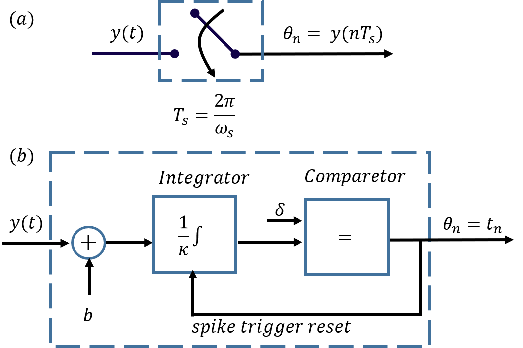
Fig. 1: (a) classical schematic sampler. (b) IF-TEM sampler.

2.2 Sampling and Recovery of BL and FRI signals

A signal $x(t)$ is said to be $c$-bounded and $2\Omega$ BL signal if $|x(t)|\leq c$, where $c\in\mathbb{R}$, and its Fourier transform decays outside the closed interval $[-\Omega,\Omega]$. The frequency upper bound $\Omega$ is known as the band limit, and its support is referred to as the bandwidth [21]. The Shannon-Nyquist theorem, which we refer to as the classical approach, states that a $2\Omega$ BL signal $y(t)$ can be perfectly recovered from its uniform samples $y(nT_{s})$, if the sampling rate is at least the Nyquist rate $\frac{\Omega}{\pi}$ [21]. Results on BL signals reconstruction from IF-TEM outputs have been considered for cases where the input signal is $2\Omega$ BL and $c$-bounded with finite energy $E$ [4, 6, 8]. A signal $x(t)\in L^{2}(\mathbb{R})$ is said to have finite energy $E\in\mathbb{R}$ if $E=\int_{-\infty}^{\infty}|x(t)|^{2}dt<\infty.$ In general, the bandwidth $2\Omega$ and the amplitude upper-bound $c$ are independent. Here, we consider BL signals with maximal energy $E$; in this case, as given in [24], the relation between $\Omega$ and $c$ is $c=\sqrt{{E\Omega}/{\pi}}$.

We consider the IF-TEM sampling and recovery mechanism as in [6] (except that the refractory period is assumed to be zero). By using an iterative approach, Lazar and Tóth showed that such signals can be perfectly recovered using an IF-TEM with parameters $\{b,\kappa,\delta\}$ if $b>c$ and [6]

$$\Delta t_{\max}<\frac{\pi}{\Omega}.$$ (3)

The bound in (3) requires a bandwidth that is inversely proportional to the time difference between the firing instants, i.e., the BL input signal can be recovered if the overall firing rate of the IF-TEM is higher than the Nyquist rate. In this case, the signal is reconstructed in a manner similar to that of a BL signal recorded with irregularly spaced amplitude samples (cf. [6, 8] for IF-TEM recovery mechanism details).

In the context of FRI signals, a kernel-based sampling framework is typically studied [22, 23]. A signal $x(t)$ is said to be a $T$-periodic FRI signal if

$$x(t)=\sum_{p\in\mathbb{Z}}\sum_{\ell=1}^{L}a_{\ell}h(t-\tau_{\ell}-pT),$$ (4)

where the FRI parameters $\{(a_{\ell},\tau_{\ell})|\tau_{\ell}\in(0,T],a_{\ell}\in\mathbb{R}\}_{\ell=1}^{L}$ are the unknown amplitudes and delays. The number of FRI pulses $L$ and the pulse shape $h(t)\in\ L^{2}(\mathbb{R})$ are known. Since $x(t)$ is $T$-periodic, it has the following Fourier series representation

$$x(t)=\sum_{k\in\mathbb{Z}}X[k]e^{jk\omega_{0}t},$$ (5)

where

$$X[k]=\frac{1}{T}H(k\omega_{0})\sum_{\ell=1}^{L}a_{\ell}e^{-jk\omega_{0}\tau_{\ell}},$$ (6)

and $\omega_{0}=\frac{2\pi}{T}$. Here $H(\omega)$ is the continuous-time Fourier transform of $h(t)$. The rate of innovation of $x(t)$, that is, the degrees of freedom per unit time interval, is $\frac{2L}{T}$.

The parameters $\{a_{\ell},\tau_{\ell}\}_{\ell=1}^{L}$ can be uniquely computed from a minimum of $2L$ and $2L+2$ Fourier series coefficients (FSCs), for the classical and IF-TEM setup respectively, by using spectral analysis methods, such as the annihilating filter (AF) [22, 23, 16, 17]. Hence, with $2L$ FSCs $X[k]$ can uniquely determine the FRI signal $x(t)$ [23]. Thus, the FRI signal reconstruction problem is reduced to uniquely determining the desired number of FSCs from the signal measurements. Reconstruction from IF-TEM outputs have been considered for cases where the FRI input is $c$-bounded and is guaranteed if the IF-TEM parameters satisfy [16, 17].

$$\frac{1}{\Delta t_{\max}}\geq\frac{2L+2}{T}.$$ (7)

This condition is similar to the classical FRI method where perfect recovery is achieved when sampling at the rate of innovation. For details on sampling and perfect reconstruction of FRI signals from classical and IF-TEM outputs, we refer to [22, 19, 17].

2.3 Problem Formulation

We consider the problem of recovering a signal $x(t)$, which can be either an FRI or BL signal, from its quantized samples for the IF-TEM and classical setup. Specifically, for FRI signals, we consider a $T$-periodic FRI signal as in (4), where our goal is to retrieve the FRI parameters $\{a_{\ell},\tau_{\ell}\}_{\ell=1}^{L}$ from quantized IF-TEM samples. In this case, the FSCs are calculated from quantized samples. For BL signals, we consider a $2\Omega$ BL and $c$-bounded signal with a fixed maximal energy $E<\infty$. Our goal is to retrieve the signal from quantized IF-TEM samples.

A generalized sampling with quantization scheme is shown in Fig. 2. Here, the input signal $x(t)$ is passed through a sampling kernel $g(t)$, which results in the signal $y(t)$. Then a set of $N$ measurements, $\{\theta_{n}\}_{n=1}^{N}$, are computed from $y(t)$. The sampler is denoted by S, and the quantizer is denoted by Q. The sampler could be either a classical instantaneous sampler as shown in Fig. 1(a) or an IF-TEM as depicted in Fig. 1(b). In the former framework, we have $\theta_{n}=y(nT_{s})$, with a suitable sampling interval $T_{s}$, whereas in the later encoding scheme the measurements are given by $\theta_{n}=t_{n}$, where $\{t_{n}\}_{n=1}^{N}$ are the time-encodings.

For the BL case, the sampling kernel is a low-pass filter or can be removed. For the FRI case, in both IF-TEM and classical settings, the sampling kernel $g(t)$ is designed such that $2L+2$ FSCs of $x(t)$ are computed from $\{\theta_{n}\}_{n=1}^{N}$ where $N\geq 2L+2$. In particular, a sum-of-sincs (SoS) filter can be used to determine the FSCs from the measurements [17, 19].

After the sampler computes the measurements $\theta_{n}$ of the signal $x(t)$, the samples are quantized. In the classical sampling scheme, the instantaneous samples $y(nT_{s})$ are quantized; in IF-TEM, the differences, $T_{n}=t_{n+1}-t_{n}$ rather than the time-encodings $t_{n}$ are quantized resulting in $f(\theta_{n})=\hat{T}_{n}$, where $\hat{T}_{n}$ denotes $T_{n}$ quantized.

Due to quantization, the signal $x(t)$ cannot be perfectly recovered. Our objective is to compare the classical and IF-TEM reconstructions by calculating the MSE of the recovered FRI and BL signals from the quantized measurements $f(\theta_{n})$. In particular, we would like to assess and analyze if there is any advantage of using IF-TEM over classical sampling when recovering FRI and/or BL signals in the presence of quantization.

Fig. 2: Generalized sampling with quantization system mode: Continuous-time signal $x(t)$ is filtered through a sampling kernel $g(t)$ resulting in $y(t)$. Then $y(t)$ is sampled by using a sampler $S$ that results in a discrete representation $\{\theta_{n}\}$. The representation is quantized by a quantizer $Q$, resulting in $\{f(\theta_{n})\}$.

3 Quantized IF-TEM System

In this section, we analyze quantization strategies for classical and IF-TEM sampling schemes with FRI and BL signals. We show that as the number of pulses $L$ increases for FRI signals, or the signal’s frequency for BL signals, the dynamic range of each sample decreases. We therefore suggest increasing the resolution of the quantizer as a function of $L$ or the frequency of the signals.

For both FRI and BL signals, the sampled signal is quantized by an identical uniform scalar quantizer with resolution of $\log_{2}K$ bits, i.e., each quantizer can produce $K$ distinct output values. To compare both the IF-TEM and classical methods, first, we discuss quantization in the classic framework. For FRI signals, given that the SoS filter is bounded, the filter $y(t)$ is also bounded [17, 24]:

$$|y(t)|\leq c={L\,\,a_{\max}\,\,\|g\|_{\infty}\|h\|_{1}}.$$ (8)

For BL signals, assuming $y(t)$ is a signal with finite energy $E$ [24],

$$|y(t)|\leq c=\sqrt{\frac{E\Omega}{\pi}}.$$ (9)

This implies that the dynamic range of the instantaneous samples $y(nT_{s})$ lie within $[-c,c]$. Consider a $K$ level uniform quantizer. The quatization step size is

$$\Delta_{\text{classic}}=\frac{2c}{K}.$$ (10)

For the IF-TEM sampler, we quantize the time-differences $T_{n}$. From (2), we note that the dynamic range of $T_{n}$ is $\left[\frac{\kappa\delta}{b+c},\frac{\kappa\delta}{b-c}\right]$. Hence, for a $K$-level uniform quantizer, the step-size is given by

$$\Delta_{\text{IF-TEM}}=\frac{\frac{\kappa\delta}{b-c}-\frac{\kappa\delta}{b+c}}{K}=\frac{\kappa\delta}{(b+c)(b-c)}\frac{2c}{K}.$$ (11)

Before we proceed, note that the integrator constant $\kappa$ is a parameter of the integrator circuit, which is usually fixed. In practice, the threshold $\delta$, which is a parameter of the comparator, and the bias $b$ are easier to control. For FRI signals recovery from IF-TEM sampler, using (7), requires a the number of samples $N\geq 2L+2$. When increasing $L$, we can increase the bias $b$ or decrease the threshold $\delta$ to have a sufficient number of samples for recovery. To analyze the relation between $L$ and $\Delta_{\text{IF-TEM}}$, fixed values of $\delta$ and $\kappa$ are assumed, while $b$ can be change. We show that by increasing $L$, the quantization step size $\Delta_{\text{IF-TEM}}$ decreases. We summarize this result in the following theorem.

Theorem 1.

Consider an IF-TEM sampler followed by a K-level uniform quantizer. For FRI signals, the quantization step $\Delta_{\text{IF-TEM}}$ decreases as the number of input pulses $L$ increases.

Proof.

For fixed values of $\kappa$ and $\delta$, and since the bias is chosen such that $b>c$, substituting $b=\alpha c$ with fixed $\alpha>1$ to (11), we have

$$\Delta_{\text{IF-TEM}}=\frac{2\kappa\delta}{(\alpha+1)(\alpha-1)}\frac{2}{cK}.$$ (12)

Using (8), with an increasing number of pulses $L$, the IF-TEM quantization step size will decrease. ∎

Comparing (10) and (12), we observe that the quantization step size in classical sampling increases with the amplitude of the FRI signal; whereas in the IF-TEM framework, the step size decreases with amplitude. Note that for a fixed $K$, increasing $L$ for an FRI signal increases the number of samples $N$ in both IF-TEM and classical methods. Thus, the total number of bits will be increased in both methods. For comparison, we set the number of samples to be equal using (7).

Next, we analyze the quantization strategies for BL signals with maximal energy $E$. Similar to the FRI quantizer, a $K$-level uniform quantizer with a quantization step size $\Delta_{\text{IF-TEM}}$ and $\Delta_{\text{classic}}$ for IF-TEM and classical sampler is used. We show that by increasing $\Omega$, the quantization step size $\Delta_{\text{IF-TEM}}$ decreases.

Theorem 2.

Consider an IF-TEM sampler followed by a K-level uniform quantizer. For BL signals signals, the quantization step $\Delta_{\text{IF-TEM}}$ decreases as the frequency of the input signal increases.

Proof.

The proof directly follows using similar arguments as in Theorem 1. Substituting (9) into (12), when the input signal frequency increases, namely, increasing $\Omega$, the quantization step $\Delta_{\text{IF-TEM}}$ decreases. ∎

In the next section, we demonstrate Theorems 1 and 2. See Fig. 3, Fig. 4 and Table 1.

Note that FRI signals are determined by a finite number $L$ of unknowns, referred to as innovations, per time interval $T$. BL signals, have $L=1$ innovations per Nyquist interval $T=\frac{1}{f_{nyq}}=\frac{1}{2\Omega}$. Thus, increasing $\Omega>0$ means decreasing $T$, which causes a similar effect of reducing the quantization step size to increase $L$. The time instances become closer, which causes smaller values of $T_{n}$s. Thus, the quantization error can be reduced based on dense quantization, and the IF-TEM framework results in lower quantization error than the classical scheme.

4 Evaluation results

In this section, first, we exemplify our main result in an experimental study using simulations. We demonstrate that the quantizer resolution for each sample increases using the same number of bits overall as the input frequency increases. Next, we evaluate the performance of the proposed IF-TEM sampling frameworks with quantization in terms of MSE and compare it to the classical method and show that quantization using IF-TEM improves the recovery of FRI signals in comparison with classical sampling.

We verify our main result using a BL signal $x(t)$ as input. We consider a $2\Omega$ bandlimited signal $x(t)$ which is bounded in time, i.e., $|x(t)|\leq c$, for $c=\sqrt{(E\Omega)/\pi}$ with $E=1.6$ and $\Omega$ varying from $5-50$ Hz. We investigate the recovery after quantization for the IF-TEM and the Nyquist method. The input signal is given by

$$x(t)=\sum_{n=-N}^{N}c[n]\operatorname{sinc}\left(\frac{t-nT_{s}}{T_{s}}\right),$$ (13)

where $N=3$, $T_{s}=\frac{1}{2\Omega}$, and $c_{n}$ is randomly selected 100 times within the range $[-1,1]$. The IF-TEM parameters are selected as follows; we use fixed values of $\delta=0.075$ and $\kappa=0.4$. To have a sufficient number of samples needed for recovery, the bias is selected such that $b=6c$, resulting in a maximal oversampling factor of 3.5. We demonstrate that the time instances differences and their range, $\Delta t_{\min}-\Delta t_{\max}$, decreases as the frequency of the signal increases. Thus, as the BL signals frequency is higher, one can increase the resolution of the quantizer using the same number of bits. The results are shown in Fig. 3 and Table 1.

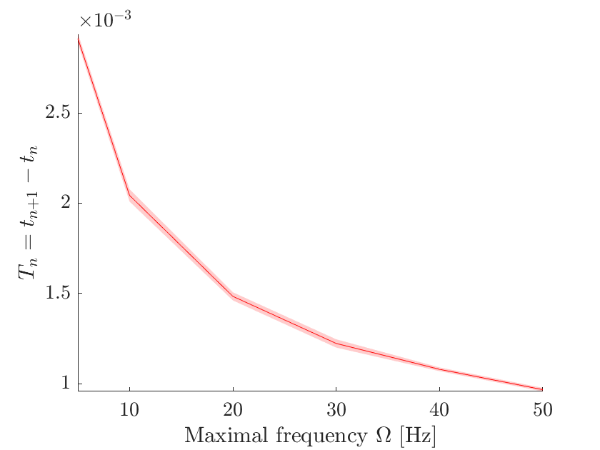
Fig. 3: Time instances differences in IF-TEM with BL signals as a function of the frequency band. The solid line shows the average $T_{n}$ and the shaded region captures the standard deviation. See the range in Table 1.

Table 1: Time instants range in IF-TEM with BL signals.

Frequency [HZ]	$5$	$10$	$30$	$50$
$\Delta t_{\min}-\Delta t_{\max}$	$9e{-04}$	$7e{-04}$	$4e{-04}$	$3e{-04}$

The suggested IF-TEM sampling framework with quantization is then evaluated in terms of MSE and compared to the conventional approach using an FRI signal model. In particular, we consider an FRI signal $x(t)$ as in (4), with period $T=1$ seconds which consists of $L=3$, $L=4$, and $L=8$ impulses, with 500 randomly selected amplitudes within the range $[-1,1]$. The time-delays are selected randomly within the range $(0,1]$ with a resolution grid of $0.05$. For both the classical and IF-TEM FRI schemes, we consider an SoS sampling kernel that aids in selecting $2L$ FSCs [17]. For each signal $|x(t)|\leq c$, where $c$ is defined in (8), the IF-TEM parameters are chosen as follows: $b=10c$, $\delta=30$, and $\kappa\in\{0.5,2\}$ for $L=3,4$ and $L=8$ respectively. The number of samples is the same for each data point in the classical and IF-TEM schemes and is approximately $8L$. After computing the FSCs of $x(t)$, the FRI parameters are computed by applying orthogonal matching pursuit to both classical and IF-TEM methods [23]. Reconstruction accuracy of the two methods is compared in terms of MSE, given by

$$\text{MSE}=\frac{||{x(t)-\bar{x}(t)}||_{L_{2}[0,T]}}{||{x(t)}||_{L_{2}[0,T]}},$$ (14)

where $\bar{x}(t)$ is the reconstructed signal.

In Fig. 4, a comparison between the expected MSE of the recovered signals from the IF-TEM sampler (in red) and the classical sampler (in blue) is shown. In the IF-TEM, the difference between the time instances is quantized, whereas, in the conventional method, the amplitudes are quantized. For each data point, the same number of samples and bits are used. First, as shown in Fig. 4, using the IF-TEM sampler results in MSE reduction of at least 5dB less using up to 8 bits, compared to the classical sampler. When the number of bits is greater than 8, almost perfect recovery is achieved in both methods. Second, when increasing the number of pulses $L$, or raising the rate of innovation, the MSE is further decreased. As increasing the number of pulses for FRI signals is similar to increasing the input signal frequency for BL signals, the same behaviour holds for BL signals.

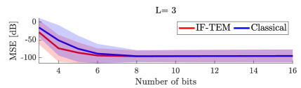
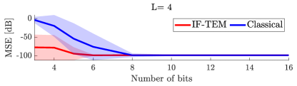
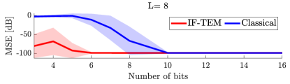
Fig. 4: Mean-squared error in estimating an FRI signal as a function of the number of bits. The solid line shows the average error and the shaded region captures the standard deviation in the estimate.

5 Conclusion

In this work we studied the problem of time-based quantization for FRI and BL signals using a uniform design of the quantization levels. We analyzed the quantizer resolution for the IF-TEM sampler and showed that using an IF-TEM sampler, in contrast to traditional sampling methods, increasing the frequency of the IF-TEM input for BL signals or the number of pulses in FRI models reduces the quantization step size using the same amount of bits. Thus, in terms of MSE, the recovery can be improved compared to the classical approaches.

References

- [1] M. Miśkowicz and D. Kościelnik, “The dynamic range of timing measurements of the asynchronous Sigma-Delta modulator,” Proc. IFAC, vol. 39, no. 21, pp. 395–400, 2006.
- [2] D. Kościelnik and M. Miśkowicz, “Designing Time-to-Digital Converter for Asynchronous ADCs,” Proc. IEEE Design Diag. Electron. Circuits Syst., pp. 1–6, 2007.
- [3] M. Miśkowicz, Event-based control and signal processing, CRC press, 2018.
- [4] A. A. Lazar and L. T. Tóth, “Perfect recovery and sensitivity analysis of time encoded bandlimited signals,” IEEE Trans. Circuits Syst. I, vol. 51, no. 10, pp. 2060–2073, 2004.
- [5] D. Kościelnik and M. Miśkowicz, “Asynchronous Sigma-Delta analog-to digital converter based on the charge pump integrator,” Analog Integr. Circuits Signal Process., vol. 55, no. 3, pp. 223–238, 2008.
- [6] A. A. Lazar, “Time encoding with an integrate-and-fire neuron with a refractory period,” Neurocomputing, vol. 58, pp. 53–58, 2004.
- [7] N. Sayiner, H. V. Sorensen, and T. R. Viswanathan, “A level-crossing sampling scheme for A/D conversion,” IEEE Trans. Circ. Syst. II, vol. 43, no. 4, pp. 335–339, 1996.
- [8] K. Adam, A. Scholefield, and M. Vetterli, “Sampling and reconstruction of bandlimited signals with multi-channel time encoding,” IEEE Tran. Signal Process., vol. 68, pp. 1105–1119, 2020.
- [9] R. Alexandru and P. L. Dragotti, “Reconstructing classes of non-bandlimited signals from time encoded information,” IEEE Trans. Signal Process., vol. 68, pp. 747–763, 2019.
- [10] Hans G Feichtinger, José C Príncipe, José Luis Romero, Alexander Singh Alvarado, and Gino Angelo Velasco, “Approximate reconstruction of bandlimited functions for the integrate and fire sampler,” Adv. Comput. Math., vol. 36, no. 1, pp. 67–78, 2012.
- [11] M. Rastogi, A. Singh Alvarado, J. G. Harris, and J. C. Príncipe, “Integrate and fire circuit as an ADC replacement,” in Proc. IEEE Int. Symp. Circuits Syst., 2011, pp. 2421–2424.
- [12] S. Ryu, C. Y. Park, W. Kim, S. Son, and J. Kim, “A Time-Based Pipelined ADC Using Integrate-and-Fire Multiplying-DAC,” IEEE Trans. Circuits Syst. I, vol. 68, no. 7, pp. 2876–2889, 2021.
- [13] B. Rajendran, A. Sebastian, M. Schmuker, N. Srinivasa, and E. Eleftheriou, “Low-Power Neuromorphic Hardware for Signal Processing Applications: A Review of Architectural and System-Level Design Approaches,” IEEE Signal Process. Mag., vol. 36, no. 6, pp. 97–110, 2019.
- [14] F. Barranco, C. Fermüller, and Y. Aloimonos, “Contour Motion Estimation for Asynchronous Event-Driven Cameras,” Proc. IEEE, vol. 102, no. 10, pp. 1537–1556, 2014.
- [15] D. Gontier and M. Vetterli, “Sampling based on timing: Time encoding machines on shift-invariant subspaces,” Applied and Comput. Harmonic Anal., vol. 36, no. 1, pp. 63–78, 2014.
- [16] S. Rudresh, A. J. Kamath, and C. S. Seelamantula, “A Time-Based Sampling Framework for Finite-Rate-of-Innovation Signals,” in Proc. IEEE Int. Conf. Acoust., Speech and Signal Process. (ICASSP), 2020, pp. 5585–5589.
- [17] H. Naaman, S. Mulleti, and Y. C. Eldar, “FRI-TEM: Time Encoding Sampling of Finite-Rate-of-Innovation Signals,” arXiv preprint arXiv:2106.05564, 2021.
- [18] O. Bar-Ilan and Y. C Eldar, “Sub-Nyquist radar via Doppler focusing,” IEEE Trans. Signal Process., vol. 62, no. 7, pp. 1796–1811, 2014.
- [19] R. Tur, Y. C. Eldar, and Z. Friedman, “Innovation rate sampling of pulse streams with application to ultrasound imaging,” IEEE Trans. Signal Process., vol. 59, no. 4, pp. 1827–1842, 2011.
- [20] I. Maravic, J. Kusuma, and M. Vetterli, “Low-sampling rate UWB channel characterization and synchronization,” J. Commun. Networks, vol. 5, no. 4, pp. 319–327, 2003.
- [21] H. Nyquist, “Certain topics in telegraph transmission theory,” Trans. Amer. Inst. Electr. Engineers, vol. 47, no. 2, pp. 617–644, 1928.
- [22] M. Vetterli, P. Marziliano, and T. Blu, “Sampling signals with finite rate of innovation,” IEEE Tran. Signal Process., vol. 50, no. 6, pp. 1417–1428, 2002.
- [23] Y. C Eldar, Sampling theory: Beyond bandlimited systems, Cambridge University Press, 2015.
- [24] A. Papoulis, “Limits on bandlimited signals,” Proc. of the IEEE, vol. 55, no. 10, pp. 1677–1686, 1967.