Deep Neural Networks and Tabular Data: A Survey

Abstract

Heterogeneous tabular data are the most commonly used form of data and are essential for numerous critical and computationally demanding applications. On homogeneous data sets, deep neural networks have repeatedly shown excellent performance and have therefore been widely adopted. However, their adaptation to tabular data for inference or data generation tasks remains highly challenging. To facilitate further progress in the field, this work provides an overview of state-of-the-art deep learning methods for tabular data. We categorize these methods into three groups: data transformations, specialized architectures, and regularization models. For each of these groups, our work offers a comprehensive overview of the main approaches. Moreover, we discuss deep learning approaches for generating tabular data, and we also provide an overview over strategies for explaining deep models on tabular data. Thus, our first contribution is to address the main research streams and existing methodologies in the mentioned areas, while highlighting relevant challenges and open research questions. Our second contribution is to provide an empirical comparison of traditional machine learning methods with eleven deep learning approaches across five popular real-world tabular data sets of different sizes and with different learning objectives. Our results, which we have made publicly available as competitive benchmarks, indicate that algorithms based on gradient-boosted tree ensembles still mostly outperform deep learning models on supervised learning tasks, suggesting that the research progress on competitive deep learning models for tabular data is stagnating. To the best of our knowledge, this is the first in-depth overview of deep learning approaches for tabular data; as such, this work can serve as a valuable starting point to guide researchers and practitioners interested in deep learning with tabular data.

I Introduction

Ever-increasing computational resources and the availability of large, labelled data sets have accelerated the success of deep neural networks[schmidhuber2015deep, deeplearningbook]. In particular, architectures based on convolutions, recurrent mechanisms [hochreiter1997long], or transformers [vaswani2017attention] have led to unprecedented performance in a multitude of domains. Although deep learning methods perform outstandingly well for classification or data generation tasks on homogeneous data (e.g., image, audio, and text data), tabular data still pose a challenge to deep learning models [arik2019tabnet, popov2019neural, Shwartz-Ziv2021, elsayed2021we]. Tabular data – in contrast to image or language data – are heterogeneous, leading to dense numerical and sparse categorical features. Furthermore, the correlation among the features is weaker than the one introduced through spatial or semantic relationships in image or speech data. Hence, it is necessary to discover and exploit relations without relying on spatial information [somepalli2021saint]. Therefore, Kadra et al. called tabular data sets the last “unconquered castle” for deep neural network models [Kadra2021reg].

Heterogeneous data are the most commonly used form of data [Shwartz-Ziv2021], and it is ubiquitous in many crucial applications, such as medical diagnosis based on patient history [ulmer2020trust, somani2021deep, borisov2021robust], predictive analytics for financial applications (e.g., risk analysis, estimation of creditworthiness, the recommendation of investment strategies, and portfolio management) [clements2020sequential], click-through rate (CTR) prediction [guo2017deepfm], user recommendation systems [zhang2019deep], customer churn prediction [ahmed2017survey, tang2020customer], cybersecurity [buczak2015survey], fraud detection [Cartella2021], identity protection [liu2021machine], psychology [urban2021deep], delay estimations [shoman2020deep], anomaly detection [pang2021deep], and so forth. In all these applications, a boost in predictive performance and robustness may have considerable benefits for both end users and companies that provide such solutions. Simultaneously, this requires handling many data-related pitfalls, such as noise, impreciseness, different attribute types and value ranges, or the missing value problem and privacy issues.

Meanwhile, deep neural networks offer multiple advantages over traditional machine learning methods. First, these methods are highly flexible [sahoo2017online], allow for efficient and iterative training, and are particularly valuable for AutoML [he2021automl, artzi2021classification, shi2021multimodal, fakoor2020fastdad, gijsbers2019open, yin2020tabert]. Second, tabular data generation is possible using deep neural networks and can, for instance, help mitigate class imbalance problems [wang2019generative]. Third, neural networks can be deployed for multimodal learning problems where tabular data can be one of many input modalities [baltruvsaitis2018multimodal, lichtenwalter2021deep, shi2021multimodal, polsterl2021combining, soares2021predicting], for tabular data distillation [medvedev2020new, li2020tnt], for federated learning [roschewitz2021ifedavg], and in many more scenarios.

Successful deployments of data-driven applications require solving several tasks, among which we identified three core challenges: (1) inference (2) data generation, and (3) interpretability. The most crucial task is inference which is concerned with making predictions based on past observations. While a powerful predictive model is critical for all the applications mentioned in the previous paragraph, the interplay between tabular data and deep neural networks goes beyond simple inference tasks. Before a predictive model can even be trained, the training data usually needs to be preprocessed. This is where data generation plays a crucial role, as one of the standard deployment steps involves the imputation of missing values [sanchez2020improving, gondara2018mida, camino2020working] and the rebalancing of the data set  [engelmann2021conditional, darabi2021synthesising] (i.e., equalizing sample sizes for different classes). Furthermore, it might be simply impossible to use the actual data due to privacy concerns, e.g., in financial or medical applications [kamthe2021copula, Choi2017medGAN]. Thus, to tackle the data preprocessing and privacy challenges, probabilistic tabular data generation is essential. Finally, with stricter data protection laws such as California Consumer Privacy Act (CCPA) [ccpa2021] and the European General Data Protection Regulation (EU GDPR) [regulation2016gdpr], which both mandate a right to explanations for automated decision systems (e.g., in the form or recourse [voigt2017eu]), interpretability is becoming a key aspect for predictive models used for tabular data [sahakyan2021explainable, GRISCI2021111]. During deployment, interpretability methods also serve as a valuable tool for model debugging and auditing [bhatt2020explainable].

Evidently, apart from the the core challenges of inference, generation, and interpretability, there are several other important subfields, such as working with data streams, distribution shifts, as well as privacy and fairness considerations that should not be neglected. Nevertheless, to navigate the vast body of literature, we focus on the identified core problems and thoroughly review the state of the art in this work. We will briefly discuss the remaining topics at the end of this survey.

Beyond reviewing current literature, we think that an exhaustive comparison between existing deep learning approaches for heterogeneous tabular data is necessary to put reported results into context. The variety of benchmarking data sets and the different setups often prevent comparison of results across papers. Additionally, important aspects of deep learning models, such as training and inference time, model size, and interpretability, are usually not discussed. We aim to bridge this gap by providing a comparison of the surveyed inference approaches with classical – yet very strong – baselines such as XGBoost [XGBOOST]. We open-source our code, allowing researchers to reproduce and extend our findings.

In summary, the aims of this survey are to provide:

1. a thorough review of existing scientific literature on deep learning for tabular data;

2. a taxonomic categorization of the available approaches for classification and regression tasks on heterogeneous tabular data;

3. a presentation of the state of the art and promising paths towards tabular data generation;

4. an overview of existing explanation approaches for deep models for tabular data;

5. an extensive empirical comparison of traditional machine learning methods and deep learning models on multiple real-world heterogeneous tabular data sets;

6. a discussion on the main reasons for the limited success of deep learning on tabular data;

7. a list of open challenges related to deep learning for tabular data.

Accordingly, this survey is structured as follows: We discuss related works in Section II. To introduce the reader to the field, in Section III, we provide definitions of the key terms, a brief outline of the domain’s history, and propose a unified taxonomy of current approaches to deep learning with tabular data. Section IV covers the main methods for modelling tabular data using deep neural networks. Section V presents an overview on tabular data generation using deep neural networks. An overview of explanation mechanisms for deep models for tabular data is presented in Section VI. In Section VII, we provide an extensive empirical comparison of machine and deep learning methods on real-world data, that also involves model size, runtime, and interpretability. In Section LABEL:sec:discussion, we summarize the state of the field and give future perspectives. Finally, we outline several open research questions before concluding in Section LABEL:sec:conclusion.

Contents

1. I Introduction
2. II Related Work
3. III Tabular Data and Deep Neural Networks
   1. III-A Definitions
   2. III-B A Brief History of Deep Learning on Tabular Data
   3. III-C Challenges of Learning With Tabular Data
   4. III-D Unified Taxonomy
4. IV Deep Neural Networks for Tabular Data
   1. IV-A Data Transformation Methods
      1. IV-A1 Single-Dimensional Encoding
      2. IV-A2 Multi-Dimensional Encoding
   2. IV-B Specialized Architectures
      1. IV-B1 Hybrid Models
      2. IV-B2 Transformer-based Models
   3. IV-C Regularization Models
5. V Tabular Data Generation
   1. V-A Methods
   2. V-B Assessing Generative Quality
6. VI Explanation Mechanisms for Deep Learning with Tabular Data
   1. VI-A Feature Highlighting Explanations
   2. VI-B Counterfactual Explanations
7. VII Experiments
   1. VII-A Data Sets
   2. VII-B Open Performance Benchmark on Tabular Data

II Related Work

To the best of our knowledge, there is no study dedicated exclusively to the application of deep neural networks to tabular data, spanning the areas of supervised and unsupervised learning, data synthesis, and interpretability. Prior works cover some of these aspects, but none of them systematically discusses the existing approaches in the broadness of this survey.

However, there are some works that cover parts of the domain. There is a comprehensive analysis of common approaches for categorical data encoding as a preprocessing step for deep neural networks by Hancock & Khoshgoftaar [hancock2020survey]. The authors compared existing methods for categorical data encoding on various tabular data sets and different deep learning architectures. We also discuss the key categorical data encoding methods in Section IV-A1.

A recent survey by Sahakyan et al. [sahakyan2021explainable] summarizes explanation techniques in the context of tabular data. Hence, we do not provide a detailed discussion of explainable machine learning for tabular data in this paper. However, for the sake of completeness, we present some of the most relevant works in Section VI and highlight open challenges in this area.

Gorishniy et al. [gorishniy2021revisiting] empirically evaluated a large number of state-of-the-art deep learning approaches for tabular data on a wide range of data sets. The authors demonstrated that a tuned deep neural network model with a ResNet-like architecture [he2016deep] shows comparable performance to some state-of-the-art deep learning approaches for tabular data.

Recently, Shwartz-Ziv & Armon [Shwartz-Ziv2021] published a study on several different deep models for tabular data including TabNet [arik2019tabnet], NODE [popov2019neural], Net-DNF [katzir2021netdnf]. Additionally, they compared deep learning approaches to gradient boosting decision tree algorithms regarding accuracy, training effort, inference efficiency, and hyperparameter optimization time. They observed that deep models had the best results on their chosen data sets, however, not one single deep model could outperform all the others in general. The deep models were challenged by gradient boosting decision trees, leading the authors to conclude that efficient tabular data modelling using deep neural networks is still an open research problem. In the face of this evidence, we aim to integrate the necessary background for future research on the inference problem and on the intertwined challenges of generation and explainability into a single work.

Figure 1: Unified taxonomy of deep neural network models for heterogeneous tabular data.

III Tabular Data and Deep Neural Networks

III-A Definitions

In this section, we give definitions for central terms used in this work. We also provide pointers to the original works for more detailed explanations of the methods.

The key concept in this survey is a (deep) neural network. Unless stated otherwise we use this concept as a synonym for feed-forward networks, as described by [deeplearningbook], and name the concrete model whenever we deviate from this concept. A deep neural network defines a mapping $\hat{f}$,

$$y=f(x)\approx\hat{f}(x;W),$$ (1)

that learns the value of the model parameters $W$ (i.e., the “weights” of a neural network) that results in the best approximation of the true underlying and unknown function $f$. In this case, $x$ is a multi-dimensional data sample (i.e., $x\in\mathbb{R}^{n}$) with corresponding target $y$ (where typically, $y\in\mathbb{R}^{k}$ for $k$ classes and $y\in\mathbb{R}$ for regression tasks) from a data set of tuples $\left\{\left(x_{i},y_{i}\right)\right\}_{i\in\mathcal{I}}$. The network is called feed-forward if the input information flows in one direction to the output without any feedback connections.

Throughout this survey we focus on heterogeneous data which usually contains a variety of attribute types – These include both continuous and discrete attributes of different type (e.g., binary values, ordinal values, high-cardinality categorical values). This is fundamentally different from homogeneous data modalities, such as images, audio, or text data where only a single feature type is present.

Categorical variables are an attribute type of particular importance. According to Lane’s definition [statistics2003Lane], categorical variables are qualitative values. They “do not imply a numerical ordering”, unlike quantitative values, which are “measured in terms of numbers”. Usually, a categorical variable can take one out of a limited set of values. Examples of typical categorical variables include gender, user_id, product_type and topic.

Tabular data, sometimes also called structured data [ryan2020deep], is a subcategory of the heterogeneous data format that is usually presented in a table [cvitkovic2020deep] with data points as rows and features as columns. In summary, for the scope of this work, we refer to a data set with a fixed number of features that are either continuous or categorical as tabular. Each data point can be understood as a row in the table, or – taking a probabilistic view – as a sample from the unknown joint distribution. An illustrative example of five rows of a heterogeneous, tabular data is provided in Table I.

TABLE I: An example of a heterogeneous tabular data set. Here we show five samples with selected variables from the Adult data set [Dua:2019]. Section VII-A provides further details on this data set.

III-B A Brief History of Deep Learning on Tabular Data

Tabular data are one of the oldest forms of data to be statistically analysed. Before digital collection of text, images, and sound was possible, almost all data were tabular  [miles1881sunstroke, fisher1936use, jdanov2019human]. Therefore, it was the target of early machine learning research [fix1951discriminatory]. However, deep neural networks became popular in the digital age and were further developed with a focus on homogeneous data. In recent years, various supervised, self-supervised, and semi-supervised deep learning approaches have been proposed that explicitly address the issue of tabular data modelling again. Early works mostly focused on data transformation techniques for preprocessing [giles1992learning, horne1995experimental, willenborg1996statistical], which are still important today [hancock2020survey].

A huge stimulus was the rise of e-commerce, which demanded novel solutions, especially in advertising [richardson2007predicting, guo2017deepfm]. These tasks required fast and accurate estimation on heterogeneous data sets with many categorical variables, for which the traditional machine learning approaches are not well suited (e.g., categorical features that have high cardinality can lead to very sparse high-dimensional feature vectors and non-robust models). As a result, researchers and data scientists started looking for more flexible solutions, e.g., those based on deep neural networks, that can capture complex non-linear dependencies in the data.

In particular, the click-through rate prediction problem has received a lot of attention [guo2017deepfm, ke2019deepgbm, wang2021masknet]. A large variety of approaches were proposed, most of them relying on specialized neural network architectures for heterogeneous tabular data.

A more recent line of research, sparked by Shavitt & Segal [shavitt2018regularization], evolved based on the idea that regularization may improve the performance of deep neural networks on tabular data [Kadra2021reg]. This has led to an intensification of research on regularization approaches.

Due to the tremendous success of attention-based approaches such as transformers on textual [brown2020language] and visual data [dosovitskiy2021visiontransformer, khan2021transformers], researchers have recently also started applying attention-based methods and self-supervised learning techniques to tabular data. After the introduction of transformer architectures to the field of tabular data [arik2019tabnet], a lot of research effort has focused on transformer architectures that can be successfully applied to very large tabular data sets.

III-C Challenges of Learning With Tabular Data

As we have mentioned in Section II, deep neural networks often perform less favourably compared to more traditional machine learning methods (e.g., tree-based methods) when dealing with tabular data. However, it is often unclear why deep learning cannot achieve the same level of predictive quality as in other domains such as image classification and natural language processing. In the following, we identify and discuss four possible reasons:

1. Low-Quality Training Data: Data quality is a common issue with real-world tabular data sets. They often include missing values [sanchez2020improving], extreme data (outliers) [pang2021deep], erroneous or inconsistent data [karr2006data], and have small overall size relative to the high-dimensional feature vectors generated from the data [Xu2018TGAN]. Also, due to the expensive nature of data collection, tabular data are frequently class-imbalanced. These challenges affect all machine learning algorithms; however, most of the modern decision tree-based algorithms can handle missing values or different/extreme variable ranges internally by looking for appropriate approximations and split values [XGBOOST, ke2017lightgbm, prokhorenkova2018catboost].

2. Missing or Complex Irregular Spatial Dependencies: There is often no spatial correlation between the variables in tabular data sets [Zhu2021igtd], or the dependencies between features are rather complex and irregular. When working with tabular data, the structure and relationships between its features have to be learned from scratch. Thus, the inductive biases used in popular models for homogeneous data, such as convolutional neural networks, are unsuitable for modelling this data type [katzir2021netdnf, rahaman2019spectral, mitchell2017spatial].

3. Dependency on Preprocessing: A key advantage of deep learning on homogeneous data is that it includes an implicit representation learning step [GoodfellowDLBook2016], so only a minimal amount of preprocessing or explicit feature construction is required. However, for tabular data and deep neural networks the performance may strongly depend on the selected preprocessing strategy [gorishniy2022embeddings]. Handling the categorical features remains particularly challenging [hancock2020survey] and can easily lead to a very sparse feature matrix (e.g., by using a one-hot encoding scheme) or introduce a synthetic ordering of previously unordered values (e.g., by using an ordinal encoding scheme). Lastly, preprocessing methods for deep neural networks may lead to information loss, leading to a reduction in predictive performance [fitkov2012evaluating].

4. Importance of Single Features: While typically changing the class of an image requires a coordinated change in many features, i.e., pixels, the smallest possible change of a categorical (or binary) feature can entirely flip a prediction on tabular data [shavitt2018regularization]. In contrast to deep neural networks, decision-tree algorithms can handle varying feature importance exceptionally well by selecting a single feature and appropriate threshold (i.e., splitting) values and “ignoring” the rest of the data sample. Shavitt & Segal [shavitt2018regularization] have argued that individual weight regularization may mitigate this challenge and motivated more work in this direction [Kadra2021reg].

With these four fundamental challenges in mind, we continue by organizing and discussing the strategies developed to address them. We start by developing a suitable taxonomy.

III-D Unified Taxonomy

In this section, we introduce a taxonomy of approaches that allows for a unified view of the field. We divide the works from the deep learning with tabular data literature into three main categories: data transformation methods, specialized architectures, and regularization models. In Fig. 1, we provide an overview of our taxonomy of deep learning methods for tabular data.

Data transformation methods. The methods in the first group transform categorical and numerical data. This is usually done to enable deep neural network models to better extract the information signal. Methods from this group do not require new architectures or adaptations of the existing data processing pipeline. Nevertheless, the transformation step comes at the cost of an increased preprocessing time. This might be an issue for high-load systems [baylor2017tfx], particularly in the presence of categorical variables with high cardinality and growing data set size. We can further subdivide this area into Single-Dimensional Encodings and Multi-Dimensional Encodings. The former encodings are employed to transform each feature independently while the latter encoding methods map an entire record to another representation.

Specialized architectures. The biggest share of works investigates specialized architectures and suggests that a different deep neural network architecture is required for tabular data. Two types of architectures are of particular importance: hybrid models fuse classical machine learning approaches (e.g., decision trees) with neural networks, while transformer-based models rely on attention mechanisms.

Regularization models. Lastly, the group of regularization models claims that one of the main reasons for the moderate performance of deep learning models on tabular data is their extreme non-linearity and model complexity. Therefore, strong regularization schemes are proposed as a solution. They are mainly implemented in the form of special-purpose loss functions.

We believe our taxonomy may help practitioners find the methods of choice that can be easily integrated into their existing tool chain. For instance, applying data transformations can result in performance improvements while maintaining the current model architecture. Conversely, using specialized architectures, the data preprocessing pipeline can be kept intact.

IV Deep Neural Networks for Tabular Data

In this section, we discuss the use of deep neural networks on tabular data for classification and regression tasks according to the taxonomy presented in the previous section. We provide an overview of existing deep learning approaches in this area of research in Table II and examine the three methodological categories in detail: data transformation methods (see Subsection IV-A), architecture-based methods (see Subsection IV-B), and regularization-based models (see Subsection IV-C).

	Method	Interpretability	Key Characteristics
Encoding	SuperTML [sun2019supertml]		Transform tabular data into images for CNNs
	VIME [yoon2020vime]		Self-supervised learning and contextual embedding
	IGTD [Zhu2021igtd]		Transform tabular data into images for CNNs
	SCARF [bahri2021scarf]		Self-supervised contrastive learning
Architectures, Hybrid	Wide&Deep [cheng2016wide]		Embedding layer for categorical features
	DeepFM [guo2017deepfm]		Factorization machine for categorical data
	SDT [frosst2017distilling]	✓	Distill neural network into interpretable decision tree
	xDeepFM [lian2018xdeepfm]		Compressed interaction network
	TabNN [Ke2019tabnn]		DNNs based on feature groups distilled from GBDT
	DeepGBM [ke2019deepgbm]		Two DNNs, distill knowlegde from decision tree
	NODE [popov2019neural]		Differentiable oblivious decision trees ensemble
	NON [luo2020NON]		Network-on-network model
	DNN2LR [liu2020dnn2lr]		Calculate cross feature wields with DNNs for LR
	Net-DNF [katzir2021netdnf]		Structure based on disjunctive normal form
	Boost-GNN [Ivanov2021bgnn]		GNN on top decision trees from the GBDT algorithm
	SDTR [Luo2021sdtr]		Hierarchical differentiable neural regression model
Architectures, Transformer	TabNet [arik2019tabnet]	✓	Sequential attention structure
	TabTransformer [Huang2020tabtrans]	✓	Transformer network for categorical data
	SAINT [somepalli2021saint]	✓	Attention over both rows and columns
	ARM-Net [cai2021arm]		Adaptive relational modelling with multi-headgated attention network
	Non-Param. Transformer [kossen2021selfattention]		Process the entire dataset at once, use attention between data points
Regul.	RLN [shavitt2018regularization]	✓	Hyperparameters regularization scheme
	Regularized DNNs [Kadra2021reg]		A ”cocktail” of regularization techniques

TABLE II: Overview of deep learning approaches for tabular data. We organize them in categories ordered chronologically inside the groups. The “Interpretability” column indicates whether the approach offers some form interpretability for the model’s decisions. The key characteristics of every model are summarized in the last column.

IV-A Data Transformation Methods

Most traditional approaches for deep neural networks on tabular data fall into this group. Interestingly, data preprocessing plays a relatively minor role in computer vision, even though the field is currently dominated by deep learning solutions [deeplearningbook]. There are many different possibilities to transform tabular data, and each may have a different impact on the learning results [hancock2020survey].

IV-A1 Single-Dimensional Encoding

One of the critical obstacles for deep learning with tabular data are categorical variables. Since neural networks only accept real number vectors as inputs, these values must be transformed before a model can use them. Therefore, the first class of methods attempts to encode categorical variables in a way suitable for deep learning models.

Approaches in this group [hancock2020survey] are divided into deterministic techniques, which can be used before training the model, and more complicated automatic techniques that are part of the model architecture. There are many ways for deterministic data encoding; hence we restrict ourselves to the most common ones without the claim of completeness.

The simplest data encoding technique might be ordinal or label encoding. Every category is just mapped to a discrete numeric value, e.g., $\left\{\texttt{Apple},~{}\texttt{Banana}\right\}$ are encoded as $\left\{0,1\right\}$. One drawback of this method may be that it introduces an artificial order to previously unordered categories. Another straightforward method that does not induce any order is the one-hot encoding. One additional column for each unique category is added to the data. Only the column corresponding to the observed category is assigned the value one, with the other values being zero. In our example, Apple could be encoded as (1,0) and Banana as (0,1). In the presence of a diverse set of categories in the data, this method can lead to high-dimensional sparse feature vectors and exacerbate the “curse of dimensionality” problem.

Binary encoding limits the number of new columns by transforming the qualitative data into a numerical representation (as the label encoding does) and using the binary format of the number. Again the digits, are split into different columns, but there are only $\log(c)$ new columns if $c$ is the number of unique categorical values. If we extend our example to three fruits, e.g., {Apple, Banana, Pear}, we only need two columns to represent them: (01), (10), (11).

One approach that needs no extra columns and does not include any artificial order is the so-called leave-one-out encoding. It is based on the target encoding technique proposed in the work by [MicciBarreca2001], where every category is replaced with the mean of the target variable of that category. The leave-one-out encoding excludes the current row when computing the mean of the target variable to avoid overfitting. This approach is also used in the CatBoost framework [prokhorenkova2018catboost], a state-of-the-art machine learning library for heterogeneous tabular data based on the gradient boosting algorithm [friedman2002stochastic].

A different strategy is hash-based encoding. Every category is transformed into a fixed-size value via a deterministic hash function. The output size is not directly dependent on the number of input categories but can be chosen manually.

IV-A2 Multi-Dimensional Encoding

A first automatic encoding strategy is the VIME approach [yoon2020vime]. The authors propose a self- and semi-supervised deep learning framework for tabular data that trains an encoder in a self-supervised fashion by using two pretext tasks. Those tasks that are independent from the concrete downstream task which the predictor has to solve. The first task of VIME is called mask vector estimation; its goal is to determine which values in a sample are corrupted. The second task, i.e., feature vector estimation, is to recover the original values of the sample. The encoder itself is a simple multilayer perceptron. This automatic encoding makes use of the fact that there is often much more unlabelled than labelled data. The encoder learns how to construct an informative homogeneous representation of the raw input data. In the semi-supervised step, a predictive model, which is also a deep neural network model, is trained using the labelled and unlabelled data transformed by the encoder. For the encoder, a novel data augmentation method is used, corrupting an unlabelled data point multiple times with different masks. On the predictions from all augmented samples from one original data point, a consistency loss $\mathcal{L}_{u}$ can be computed that rewards similar outputs. Combined with a supervised loss $\mathcal{L}_{s}$ from the labelled data, the predictive model minimizes the final loss $\mathcal{L}=\mathcal{L}_{s}+\beta\cdot\mathcal{L}_{u}.$ To summarize, the VIME network trains an encoder, which is responsible to transform the categorical and numerical features into a new homogeneous and informative representation. This transformed feature vector is used as an input to the predictive model. For the encoder itself, the categorical data can be transformed by a simple one-hot-encoding and binary encoding.

Another stream of research aims at transforming the tabular input into a more homogeneous format. Since the revival of deep learning, convolutional neural networks have shown tremendous success in computer vision tasks. Therefore, the work by [sun2019supertml] proposed the SuperTML method, which is a data conversion technique to transform tabular data into an image data format (2-d matrices), i.e., black-and-white images.

The image generator for tabular data (IGTD) by [Zhu2021igtd] follows an idea similar to SuperTML. The IGTD framework converts tabular data into images to make use of classical convolutional architectures. As convolutional neural networks rely on spatial dependencies, the transformation into images is optimized by minimizing the difference between the feature distance ranking of the tabular data and the pixel distance ranking of the generated image. Every feature corresponds to one pixel, which leads to compact images with similar features close at neighbouring pixels. Thus, IGDTs can be used in the absence of domain knowledge. The authors show relatively solid results for data with strong feature relationships but the method may fail if the features are independent or feature similarities can not characterize the relationships. In their experiments, the authors used only gene expression profiles and molecular descriptors of drugs as data. This kind of data may lead to a favourable inductive bias, so the general viability of the approach remains unclear.

IV-B Specialized Architectures

Specialized architectures form the largest group of approaches for deep tabular data learning. Hence, in this group, the focus is on the development and investigation of novel deep neural network architectures designed specifically for heterogeneous tabular data. Guided by the types of available models, we divide this group into two sub-groups: Hybrid models (presented in IV-B1) and transformer-based models (discussed in IV-B2).

IV-B1 Hybrid Models

Most approaches for deep neural networks on tabular data are hybrid models. They transform the data and fuse successful classical machine learning approaches, often decision trees, with neural networks. We distinguish between fully differentiable models, that can be differentiated with respect to all their parameters and partly differentiable models.

Fully differentiable Models. The fully differentiable models in this category offer a valuable property: They permit end-to-end deep learning for training and inference by means of gradient descent optimizers. Thus, they allow for highly efficient implementations in modern deep learning frameworks that exploit GPU or TPU acceleration throughout the code.

Popov et al. [popov2019neural] propose an ensemble of differentiable oblivious decision trees [langley1994oblivious] – also known as the NODE framework for deep learning on tabular data. Oblivious decision trees use the same splitting function for all nodes on the same level and can therefore be easily parallelized. NODE is inspired by the successful CatBoost [prokhorenkova2018catboost] framework. To make the whole architecture fully differentiable and benefit from end-to-end optimization, NODE utilizes the entmax transformation [peters2019sparse] and soft splits. In the original experiments, the NODE framework outperforms XGBoost and other GBDT models on many data sets. As NODE is based on decision tree ensembles, there is no preprocessing or transformation of the categorical data necessary. Decision trees are known to handle discrete features well. In the official implementation, strings are converted to integers using the leave-one-out encoding scheme. The NODE framework is widely used and provides a sound implementation that can be readily deployed.

Frosst & Hinton [frosst2017distilling] contribut another model relying on soft decision trees (SDT) to make neural networks more interpretable. They investigated training a deep neural network first, before using a mixture of its outputs and the ground truth labels to train the SDT model in a second step. This also allows for semi-supervised learning with unlabelled samples that are labelled by the deep neural network and used to train a more robust decision tree along with the labelled data. The authors showed that training a neural model first increases accuracy over SDTs that are directly learned from the data. However, their distilled trees still exhibit a performance gap to the neural networks that were fitted in the initial step. Nevertheless, the model itself shows a clear relationship among different classes in a hierarchical fashion. It groups different categorical values based on the common patterns, e.g., the digits 8 and 9 from the MNIST data set [lecun-mnisthandwrittendigit-2010]. To summarize, the proposed method allows for high interpretability and efficient inference, at the cost of slightly reduced accuracy.

Follow-up work [Luo2021sdtr] extends this line of research to heterogeneous tabular data and regression tasks and presents the soft decision tree regressor (SDTR) framework. The SDTR is a neural network which imitates a binary decision tree. Therefore, all neurons, like nodes in a tree, get the same input from the data instead of the output from previous layers. In the case of deep networks, the SDTR could not beat other state-of-the-art models, but it has shown promising results in a low-memory setting, where single tree models and shallow architectures were compared.

Katzir et al. [katzir2021netdnf] follow a related idea. Their Net-DNF builds on the observation that every decision tree is merely a form of a Boolean formula, more precisely a disjunctive normal form. They use this inductive bias to design the architecture of a neural network, which is able to imitate the characteristics of the gradient boosting decision trees algorithm. The resulting Net-DNF was tested for classification tasks on data sets with no missing values, where it showed results that are comparable to those of XGBoost [XGBOOST]. However, the authors did not mention how to handle high-cardinality categorical data, as the used data sets contained mostly numerical and few binary features.

Linear models (e.g., linear and logistic regression) provide global interpretability but are inferior to complex deep neural networks. Usually, handcrafted feature engineering is required to improve the accuracy of linear models. Liu et al. [liu2020dnn2lr] use a deep neural network to combine the features in a possibly non-linear way; the resulting combination then serves as input to the linear model. This enhances the simple model while still providing interpretability.

The work by Cheng et al. [cheng2016wide] proposes a hybrid architecture that consists of linear and deep neural network models – Wide&Deep. A linear model that takes single features and a wide selection of hand-crafted logical expressions on features as an input is enhanced by a deep neural network to improve the generalization capabilities. Additionally, Wide&Deep learns an $n$-dimensional embedding vector for each categorical feature. All embeddings are concatenated resulting in a dense vector used as input to the neural network. The final prediction can be understood as a sum of both models. A similar work by Guo et al. [guo2016entity] proposes an embedding using deep neural networks for categorical variables.

Another contribution to the realm of Wide&Deep models is DeepFM [guo2017deepfm]. The authors demonstrate that it is possible to replace the hand-crafted feature transformations with learned Factorization Machines (FMs) [rendle2010factorization], leading to an improvement of the overall performance. The FM is an extension of a linear model designed to capture interactions between features within high-dimensional and sparse data efficiently. Similar to the original Wide&Deep model, DeepFM also relies on the same embedding vectors for its “wide” and “deep” parts. In contrast to the original Wide&Deep model, however, DeepFM alleviates the need for manual feature engineering.

Lastly, Network-on-Network (NON) [luo2020NON] is a classification model for tabular data, which focuses on capturing the intra-feature information efficiently. It consists of three components: a field-wise network consisting of one unique deep neural network for every column to capture the column-specific information, an across-field-network, which chooses the optimal operations based on the data set, and an operation fusion network, connecting the chosen operations allowing for non-linearities. As the optimal operations for the specific data are selected, the performance is considerably better than that of other deep learning models. However, the authors did not include decision trees in their baselines, the current state-of-the-art models on tabular data. Also, training as many neural networks as columns and selecting the operations on the fly may lead to a long computation time.

Partly differentiable Models. This subgroup of hybrid models aims at combining non-differentiable approaches with deep neural networks. Models from this group usually utilize decision trees for the non-differentiable part.

The DeepGBM model [ke2019deepgbm] combines the flexibility of deep neural networks with the preprocessing capabilities of gradient boosting decision trees. DeepGBM consists of two neural networks – CatNN and GBDT2NN. While CatNN is specialized to handle sparse categorical features, GBDT2NN is specialized to deal with dense numerical features.

In the preprocessing step for the CatNN network, the categorical data are transformed via an ordinal encoding (to convert the potential strings into integers), and the numerical features are discretized, as this network is specialized for categorical data. The GBDT2NN network distills the knowledge about the underlying data set from a model based on gradient boosting decision trees by accessing the leaf indices of the decision trees. This embedding based on decision tree leaves was first proposed by [moosmann2006fast] for the random forest algorithm. Later, the same knowledge distillation strategy has been adopted for gradient boosting decision trees [FACEBOOK].

Using the proposed combination of two deep neural networks, DeepGBM has a strong learning capacity for both categorical and numerical features. Distinctively, the authors implemented and tested DeepGBM’s online prediction performance, which is significantly higher than that of gradient boosting decision trees. On the downside, the leaf indices can be seen as meta categorical features since these numbers cannot be directly compared. Also, it is not clear how other data-related issues, such as missing values, different scaling of numeric features, and noise influence the predictions produced by the models.

The TabNN architecture, introduced by [Ke2019tabnn], is based on two principles: explicitly leveraging expressive feature combinations and reducing model complexity. It distills the knowledge from gradient boosting decision trees to retrieve feature groups; it clusters them and then constructs the neural network based on those feature combinations. Also, structural knowledge from the trees is transferred to provide an effective initialization. However, the construction of the network already takes different extensive computation steps of which one is only a heuristic to avoid an NP-hard problem. Overall, considering the construction challenges and that an implementation of TabNN was not provided, the practical use of the network seems limited.

In similar spirit to DeepGBM and TabNN, the work from [Ivanov2021bgnn] proposes using gradient boosting decision trees for the data prepossessing step. The authors show that a decision tree structure has the form of a directed graph. Thus, the proposed framework exploits the topology information from the decision trees using graph neural networks [scarselli2008graph]. The resulting architecture is coined Boosted Graph Neural Network (BGNN). In multiple experiments, BGNN demonstrates that the proposed architecture is superior to existing solid competitors in terms of predictive performance and training time.

IV-B2 Transformer-based Models

Transformer-based approaches form another subgroup of model-based deep neural methods for tabular data. Inspired by the recent surge of interest in transformer-based methods and their successes on text and visual data [wang2019language, khan2021transformers], researchers and practitioners have proposed multiple approaches using deep attention mechanisms [vaswani2017attention] for heterogeneous tabular data.

TabNet [arik2019tabnet] is one of the first transformer-based models for tabular data. Like a decision tree, the TabNet architecture comprises multiple subnetworks that are processed in a sequential hierarchical manner. According to [arik2019tabnet], each subnetwork corresponds to one decision step. To train TabNet, each decision step (subnetwork) receives the current data batch as input. TabNet aggregates the outputs of all decision steps to obtain the final prediction. At each decision step, TabNet first applies a sparse feature mask [Martins2016sparsemax] to perform soft instance-wise feature selection. The authors claim that the feature selection can save valuable resources, as the network may focus on the most important features. The feature mask of a decision step is trained using attentive information from the previous decision step. To this end, a feature transformer module decides which features should be passed to the next decision step and which features should be used to obtain the output at the current decision step. Some layers of the feature transformers are shared across all decision steps. The obtained feature masks correspond to local feature weights and can also be combined into a global importance score. Accordingly, TabNet is one of the few deep neural networks that offers different levels of interpretability by design. Indeed, experiments show that each decision step of TabNet tends to focus on a particular subdomain of the learning problem (i.e., one particular subset of features). This behaviour is similar to convolutional neural networks. TabNet also provides a decoder module that is able to preprocess input data (e.g., replace missing values) in an unsupervised way. Accordingly, TabNet can be used in a two-stage self-supervised learning procedure, which improves the overall predictive quality. One of the popular Python [van1995python] frameworks for tabular data provides an efficient implementation of TabNet [joseph2021pytorch]. Recently, TabNet has also been investigated in the context of fair machine learning [boughorbel2021fairness, mehrabi2021survey].

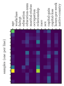
(a) TabNet attributions

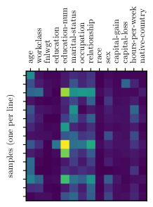
(b) KernelSHAP attributions

Figure 2: Interpretable learning with the TabNet [arik2019tabnet] architecture. We compare the attributions provided by the model for a sample from the UCI Adult data set with those provided by the game theoretic KernelSHAP framework [lundberg2017unified].

Attention-based architectures offer mechanisms for interpretability, which is an essential advantage over many hybrid models. Figure 2 shows attentions maps of the TabNet model and KernelSHAP explanation framework on the Adult data set [Dua:2019].

Another supervised and semi-supervised approach is introduced by Huang et al. [Huang2020tabtrans]. Their TabTransformer architecture uses self-attention-based transformers to map the categorical features to a contextual embedding. This embedding is more robust to missing or noisy data and enables interpretability. The embedded categorical features are then together with the numerical ones fed into a simple multilayer perceptron. If, in addition, there is an extra amount of unlabelled data, unsupervised pre-training can improve the results, using masked language modelling or replace token detection. Extensive experiments show that TabTransformer matches the performance of tree-based ensemble techniques, showing success also when dealing with missing or noisy data. The TabTransformer network puts a significant focus on the categorical features. It transforms the embedding of those features into a contextual embedding which is then used as input for the multilayer perceptron. This embedding is implemented by different multi-head attention-based transformers, which are optimized during training.

ARM-net [cai2021arm] is an adaptive neural network for relation modelling tailored to tabular data. The key idea of the ARM-net framework is to model feature interactions with combined features (feature crosses) selectively and dynamically by first transforming the input features into exponential space and then determining the interaction order and interaction weights adaptively for each feature cross. Furthermore, the authors propose a novel sparse attention mechanism to generate the interaction weights given the input data dynamically. Thus, users can explicitly model feature crosses of arbitrary orders with noisy features filtered selectively.

SAINT (Self-Attention and Intersample Attention Transformer) [somepalli2021saint] is a hybrid attention approach, combining self-attention [vaswani2017attention] with inter-sample attention over multiple rows. When handling missing or noisy data, this mechanism allows the model to borrow the corresponding information from similar samples, which improves the model’s robustness. The technique is reminiscent of nearest-neighbour classification. In addition, all features are embedded into a combined dense latent vector, enhancing existing correlations between values from one data point. To exploit the presence of unlabelled data, a self-supervised contrastive pre-training can further improve the results, minimizing the distance between two views of the same sample and maximizing the distance between different ones. Like the VIME framework (Section IV-A1), SAINT uses CutMix [yun2019cutmix] to augment samples in the input space and uses mixup [zhang2017mixup] in the embedding space.

Finally, even some new learning paradigms are being proposed. For instance, the Non-Parametric Transformer (NPT) [kossen2021selfattention] does not construct a mapping from individual inputs to outputs but uses the entire data set at once. By using attention between data points, relations between arbitrary samples can be modelled and leveraged for classifying test samples.

IV-C Regularization Models

The third group of approaches argues that extreme flexibility of deep learning models for tabular data is one of the main learning obstacles and strong regularization of learned parameters may improve the overall performance.

One of the first methods in this category was the Regularization Learning Network (RLN) proposed by Shavitt & Segal [shavitt2018regularization], which uses a learned regularization scheme. The main idea is to apply trainable regularization coefficients to each single weight in a neural network, thereby lowering the sensitivity. To efficiently determine the corresponding coefficients, the authors propose a novel loss function termed “Counterfactual Loss”. The regularization coefficients lead to a very sparse network, which also provides the importance of the remaining input features.

In their experiments, RLNs outperform deep neural networks and obtain results comparable to those of the gradient boosting decision trees algorithm, but the evaluation relies on a data set with mainly numerical data to compare the models. The RLN paper does not address the issues of categorical data. For the experiments and the example implementation data sets with exclusively numerical data (except for the gender attribute) were used. A similar idea is proposed in [borisov2019cancelout], where regularization coefficients are learned only in the first layer with a goal to extract feature importance.

Kadra et al. [Kadra2021reg] state that simple multilayer perceptrons can outperform state-of-the-art algorithms on tabular data if deep learning networks are properly regularized. The authors propose a “cocktail” of regularization with thirteen different techniques that are applied jointly. From those, the optimal subset and their subsidiary hyperparameters are selected. They demonstrate in extensive experiments that the “cocktails” regularization can not only improve the performance of multilayer perceptrons, but these simple models also outperform tree-based architectures. On the downside, the extensive per-data set regularization and hyperparameter optimization take much more computation time than the gradient boosting decision trees algorithm.

There are several other works [valdes2021lockout, fiedler2021simple, lounici2021muddling] showing that strong regularization of deep neural networks can be beneficial for tabular data.

V Tabular Data Generation

For many applications, the generation of realistic tabular data is fundamental. Two of the main purposes are data augmentation [chen2019faketables] and data imputation (i.e., the filling of missing values) [gondara2018mida, camino2020working] and rebalancing [engelmann2021conditional, Quintana2019towardsHumanComfort, koivu2020synthetic, darabi2021synthesising]. Another highly relevant topic is privacy-aware machine learning [Choi2017medGAN, Fan2020designSpace, kamthe2021copula] where generated data can potentially be leveraged to overcome privacy concerns.

V-A Methods

While the generation of images and text is highly explored [karras2020analyzing, lin2017adversarial, subramanian2017adversarial], generating synthetic tabular data is still a challenge. The mixed structure of discrete and continuous features along with their different value distributions still poses a significant challenge.

Classical approaches for the data generation task include Copulas [patki2016synthetic, li2020sync] and Bayesian Networks [zhang2017privbayes]. Among Bayesian Networks those based on the Chow-Liu approximation [chow1968approximating] are especially popular.

In the deep-learning era, Generative Adversarial Networks (GANs) [goodfellow2014generative] have proven highly successful for the generation of images [radford2015unsupervised, karras2020analyzing]. GANs were recently introduced as an original way to train a generative deep neural network model. They consist of two separate models: a generator ${G}$ that generates samples from the data distribution, and a discriminator ${D}$ that estimates the probability that a sample came from the ground truth distribution. Both ${G}$ and ${D}$ are usually chosen to be non-linear functions such as a multilayer perceptrons. To learn a generator distribution ${p_{g}}$ over data ${\bm{x}}$, the generator ${G(\bm{z};\theta_{g})}$ maps samples from a noise distribution ${p_{z}(\bm{z})}$ (e.g., the Gaussian distribution) to the input data space. The discriminator ${D(\bm{x};\theta_{d})}$ outputs the probability that a data point ${\bm{x}}$ comes from the training data’s distribution $p_{data}$ rather than from the generator’s output distribution ${p_{g}}$. During joint training of ${G}$ and ${D}$, $G$ will start generating successively more realistic samples to fool the discriminator $D$. For more details on GANs, we refer the interested reader to the original paper [goodfellow2014generative].

Although it was found that GANs lag behind at the generation of discrete outputs such as natural language [subramanian2017adversarial], they are still frequently chosen to generate tabular data. Vanilla GANs or derivates such as the Wasserstein GAN (WGAN) [arjovsky2017wasserstein], WGAN with gradient penalty (WGAN-GP) [gulrajani2017improved], Cramér GAN [bellemare2017cramer], or the Boundary seeking GAN [hjelm2017boundary], which is designed to model discrete data, are commonly used in the literature to generate tabular data. Moreover, VeeGAN [srivastava2017veegan] is frequently used for tabular data. Apart from GANs, autoencoder-based architectures – in particular those relying on Variational Autoencoders (VAEs) [Kingma2014VAE] – have been proposed [Ma2020VAEM, Xu2019CTGAN].

In Table III, we provide an overview of tabular generation approaches, that use deep learning techniques. Note that due to the enormous number of approaches, we list the most influential works that address the problem of data generation with a particular focus on tabular data. We exclude works that are targeted towards highly domain-specific tasks.

In the following section, we will briefly discuss the most relevant approaches that helped shape the domain. For example, MedGAN by [Choi2017medGAN] was one of the first works and provides a deep learning model to generate patient records. As all the features in their work are discrete, this model cannot be easily transferred to arbitrary tabular data sets. The table-GAN approach by [Park2018GAN] adapts the Deep Convolutional GAN for tabular data. Specifically, the features from one record are converted into a matrix, so that they can be processed by convolutional filters of a convolutional neural network. However, it remains unclear to which extent the inductive bias used for images are suitable for tabular data.

The approach by Xu et al. [Xu2019CTGAN] focuses on the correlation between the features of one data point. The authors first propose the mode-specific normalization technique for data preprocessing that allows to transform non-Gaussian distributions in the continuous columns. They express numeric values in terms of a mixture component number and the deviation from that component’s center. This allows to represent multi-modal and skewed distributions. Their generative solution, coined CTGAN, uses the conditional GAN architecture to enforce learning proper conditional distributions for each column. To obtain categorical values and to allow for backpropagation in the presence of categorical values, the gumbel-softmax trick [jang2016categorical] is utilized. The authors also propose a model based on Variational Autoencoders, named TVAE (Tabular Variational Autoencoder) which outperforms their suggested GAN approach. Both approaches can be considered state-of-the-art.

While GANs and VAEs are prevalent, other recently proposed architectures include machine-learned Causal Models [wen2021causal] and Invertible Flows [kamthe2021copula]. When privacy is the main factor of concern, models such as PATE-GAN [jordon2018pate] provide generative models with certain differential privacy guarantees. Although very relevant for practical applications, such privacy guarantees and related federated learning approaches with tabular data are outside the scope of this review.

Fan et al. [Fan2020designSpace] compare a variety of different GAN architectures for tabular data synthesis and recommend using a simple, fully connected architecture with a vanilla GAN loss with minor changes to prevent mode-collapse. They also use the normalization proposed by [Xu2019CTGAN]. In their experiments, the Wasserstein GAN loss or the use of convolutional architectures on tabular data does boost the generative performance.

Method	Based upon	Application
medGAN [Choi2017medGAN]	Autoencoder+GAN	Medical Records
TableGAN [Park2018GAN] DCGAN	General
Mottini et al. [Mottini2018GAN]	Cramér GAN	Passenger Records
Camino et al. [camino2018generating]	medGAN, ARAE	General
medBGAN, medWGAN [Baowaly2019GAN]	WGAN-GP, Boundary seeking GAN	Medical Records
ITS-GAN [chen2019faketables]	GAN with AE for constraints	General
CTGAN, TVAE [Xu2019CTGAN]	Wasserstein GAN, VAE	General
actGAN [koivu2020synthetic]	WGAN-GP	Health Data
VAEM [Ma2020VAEM]	VAE (Hierarchical)	General
OVAE [vardhan2020generating]	Oblivious VAE	General
TAEI [darabi2021synthesising]	AE+SMOTE (in multiple setups)	General
Causal-TGAN [zhao2021ctab]	Causal-Model, WGAN-GP	General
Copula-Flow [kamthe2021copula]	Invertible Flows	General

TABLE III: Generation of tabular data using deep neural network models (in chronological order).

V-B Assessing Generative Quality

To assess the quality of the generated data, several performance measures are used. The most common approach is to define a proxy classification task and train one model for it on the real training set and another on the artificially generated data set. With a highly capable generator, the predictive performance of the artificial-data model on the real-data test set should be almost on par with its real-data counterpart. This measure is often referred to as machine learning efficacy and used in [Choi2017medGAN, Mottini2018GAN, Xu2019CTGAN]. In non-obvious classification tasks, an arbitrary feature can be used as a label and predicted [Choi2017medGAN, camino2018generating, Baowaly2019GAN]. Another approach is to visually inspect the modelled distributions per-feature, e.g., the cumulative distribution functions [chen2019faketables] or compare the expected values in scatter plots [Choi2017medGAN, camino2018generating]. A more quantitative approach is the use of statistical tests, such as the Kolmogorov-Smirnov test [massey1951kolmogorov], to assess the distributional difference [Baowaly2019GAN]. On synthetic data sets, the output distribution can be compared to the ground truth, e.g., in terms of log-likelihood [Xu2019CTGAN, wen2021causal]. Because overfitted models can also obtain good scores, [Xu2019CTGAN] propose evaluating the likelihood of a test set under an estimate of the GAN’s output distribution. Especially in a privacy-preserving context, the distribution of the Distance to Closest Record (DCR) can be calculated and compared to the respective distances on the test set [Park2018GAN]. This measure is important to assess the extent of sample memorization. Overall, we conclude that a single measure is not sufficient to assess the generative quality. For instance, a generative model that memorizes the original samples will score well in the machine learning efficiency metric but fail the DCR check. Therefore, we highly recommend using several evaluation measures that focus on individual aspects of data quality.

VI Explanation Mechanisms for Deep Learning with Tabular Data

Explainable machine learning is concerned with the problem of providing explanations for complex machine learning models. With stricter regulations for automated decision making [regulation2016gdpr] and the adoption of machine learning models in high-stakes domains such as finance and healthcare [bhatt2020explainable], interpretability is becoming a key concern. Towards this goal, various streams of research follow different explainability paradigms. Among these, feature attribution methods and counterfactual explanations are two of the popular forms [guidotti2018survey, gade2019explainable, pawelczyk2021carla]. Because these techniques are gaining importance for researchers and practitioners alike, we dedicate the following section to reviewing these methods.

VI-A Feature Highlighting Explanations

Local input attribution techniques seek to explain the behaviour of machine learning models instance by instance. Those methods aim to highlight the influence the inputs have on the prediction by assigning importance scores to the input features. Some popular approaches for model explanations aim at constructing classification models that are explainable by design [lou2012intelligible, alvarez2018towards, wang2019designing]. This is often achieved by enforcing the deep neural network model to be locally linear. Moreover, if the model’s parameters are known and can be accessed, then the explanation technique can use these parameters to generate the model explanation. For such settings, relevance-propagation-based methods, e.g., [bach2015pixel, montavon2019layer], and gradient-based approaches, e.g., [kasneci2016licon, sundararajan2017axiomatic, chattopadhay2018grad], have been suggested. In cases where the parameters of the neural network cannot be accessed, model-agnostic approaches can prove useful. This group of approaches seeks to explain a model’s behavior locally by applying surrogate models [ribeiro2016should, lundberg2017unified, ribeiro2018anchors, lundberg2020local, haug2021baselines], which are interpretable by design and are used to explain individual predictions of black-box machine learning models. In order to test the performance of these black-box explanations techniques, Liu et al. [liu2021synthetic] suggest a python-based benchmarking library.

VI-B Counterfactual Explanations

From the perspective of algorithmic recourse, the main purpose of counterfactual explanations is to suggest constructive interventions to the input of a deep neural network so that the output changes to the advantage of an end user. In simple terms, a minimal change to the feature vector that will flip the classification outcome is computed and provided as an explanation. By emphasizing both the feature importance and the recommendation aspect, counterfactual explanation methods can be further divided into three different groups: works that assume that all features can be independently manipulated [wachter2017counterfactual] and works that focus on manifold constraints to capture feature dependencies.

In the class of independence-based methods, where the input features of the predictive model are assumed to be independent, some approaches use combinatorial solvers to generate recourse in the presence of feasibility constraints [ustun2019actionable, russell2019efficient, rawal2020individualized, karimi2019model]. Another line of research deploys gradient-based optimization to find low-cost counterfactual explanations in the presence of feasibility and diversity constraints [Dhurandhar2018, mittelstadt2019explaining, mothilal2020fat]. The main problem with these approaches is that they abstract from input correlations.

To alleviate this problem and to suggest realistic looking counterfactuals, researchers have suggested building recourse suggestions on generative models [pawelczyk2019, downs2020interpretable, joshi2019towards, mahajan2019preserving, pmlr-v124-pawelczyk20a, antoran2020getting]. The main idea is to change the geometry of the intervention space to a lower dimensional latent space, which encodes different factors of variation while capturing input dependencies. To this end, these methods primarily use (tabular data) variational autoencoders [Kingma2014VAE, nazabal2018handling]. In particular, Mahajan et al. [mahajan2019preserving] demonstrate how to encode various feasibility constraints into such models. However, an extensive comparison across this class of methods is still missing since it is difficult to measure how realistic the generated data are in the context of algorithmic recourse.

More recently, a few works have suggested to develop counterfactual explanations that are robust to model shifts and noise in the recourse implementations [upadhyay2021robust, dominguezolmedo2021adversarial, pawelczyk2022noisy]. A comprehensive treatment on how to extend these lines of work to arbitrary high cardinality categorical variables is still an open problem in the field.

For a more fine-grained overview over the literature on counterfactual explanations we refer the interested reader to the most recent surveys [karimi2020survey, verma2020counterfactual]. Finally, Pawelczyk et al. [pawelczyk2021carla] have implemented an open-source python library which provides support for many of the aforementioned counterfactual explanation models.

VII Experiments

Although several experimental studies have been published in recent years [Shwartz-Ziv2021, Kadra2021reg], an exhaustive comparison between existing deep learning approaches for heterogeneous tabular data is still missing in the literature. For example, important aspects of deep learning models such as training and inference time, model size, and interpretability, are not discussed.

To fill this gap, we present an extensive empirical comparison of machine and deep learning methods on real-world data sets with varying characteristics in this section. We discuss the data set choice (VII-A), the results (VII-B), and present a comparison of the training and inference time for all the machine learning models considered in this survey (LABEL:sec:benchtime). We also discuss the size of deep learning models. Lastly, to the best of our knowledge, we present the first comparison of explainable deep learning methods for tabular data (LABEL:sec:interpretbench). We release the full source code of our experiments for maximum transparency.

VII-A Data Sets

In computer vision, there are many established data sets for the evaluation of new deep learning architectures such as MNIST [lecun-mnisthandwrittendigit-2010], CIFAR [Krizhevsky09learningmultiple], and ImageNet [deng2009imagenet]. On the contrary, there are no established standard heterogeneous data sets. Carefully checking the works listed in Section IV, we identified over 100 different data sets with different characteristics in their respective experimental evaluation sections. We note that the small overlap between the mentioned works makes it hard to compare the results across these works in general. Therefore, in this work, we deliberately select data sets covering the entire range of characteristics, such as data domain (e.g., finance, e-commerce, geography, physics), different types of target variables (classification, regression), varying number of categorical variables and continuous variables, and differing sample sizes (small to large). Furthermore, most of the selected data sets were previously featured in multiple studies.

The first data set of our study is the Home Equity Line of Credit (HELOC) data set provided by FICO [HelocDataset]. This data set consists of anonymized information from real homeowners who applied for home equity lines of credit. A HELOC is a line of credit typically offered by a bank as a percentage of home equity. The task consists of using the information about the applicant in their credit report to predict whether they will repay their HELOC account within a two-year period.

We further use the Adult Income data set [Dua:2019], which is among the most popular tabular data sets used in the surveyed work (5 usages). It includes basic information about individuals such as: age, gender, education, etc. The target variable is binary; it represents high and low income.

The largest tabular data set in our study is HIGGS, which stems from particle physics. The task is to distinguish between signals with Higgs bosons (HIGGS) and a background process [baldi2014searching]. Monte Carlo simulations [mooney1997monte] were used to produce the data. In the first 21 columns (columns 2-22), the particle detectors in the accelerator measure kinematic properties. In the last seven columns, these properties are analyzed. In total, HIGGS includes eleven million rows. In contrast to other data sets of our study, the HIGGS data set contains only numerical or continuous variables. Since DeepFM, DeepGBM, and TabTransformer models require at least one categorical attribute, we binarize the twenty-first variable into a categorical variable with three groups.

The Covertype data set [Dua:2019] is multi-classification data set which holds cartographic information about land cells (e.g., elevation, slope). The goal is to predict which one out of seven forest cover types is present in the cell.

Finally, we utilize the California Housing data set [pace1997sparse], which contains information about a number of properties. The prediction task (regression) is to estimate price of the corresponding home.

The fundamental characteristics of the selected data sets are summarized in Table IV.

	HELOC	Adult	HIGGS	Covertype	California
		Income			Housing
Samples	9.871	32.561	11 M.	581.012	20.640
Num. features	21	6	27	52	8
Cat. features	2	8	1	2	0
Task	Binary	Binary	Binary	Multi-Class	Regression
Classes	2	2	2	7	-

TABLE IV: Main properties of the real-world heterogeneous tabular data sets used in this survey. We also indicate the data set task, where “Binary” stands for binary classification, and “Multi-class” represents multi-class classification.

VII-B Open Performance Benchmark on Tabular Data