Hypernetworks for Continual Semi-Supervised Learning

Abstract

Learning from data sequentially arriving, possibly in a non i.i.d. way, with changing task distribution over time is called continual learning. Much of the work thus far in continual learning focuses on supervised learning and some recent works on unsupervised learning. In many domains, each task contains a mix of labelled (typically very few) and unlabelled (typically plenty) training examples, which necessitates a semi-supervised learning approach. To address this in a continual learning setting, we propose a framework for semi-supervised continual learning called Meta-Consolidation for Continual Semi-Supervised Learning (MCSSL). Our framework has a hypernetwork that learns the meta-distribution that generates the weights of a semi-supervised auxiliary classifier generative adversarial network (Semi-ACGAN) as the base network. We consolidate the knowledge of sequential tasks in the hypernetwork, and the base network learns the semi-supervised learning task. Further, we present Semi-Split CIFAR-10, a new benchmark for continual semi-supervised learning, obtained by modifying the Split CIFAR-10 dataset, in which the tasks with labelled and unlabelled data arrive sequentially. Our proposed model yields significant improvements in the continual semi-supervised learning setting. We compare the performance of several existing continual learning approaches on the proposed continual semi-supervised learning benchmark of the Semi-Split CIFAR-10 dataset.

1 Introduction

Humans possess the remarkable capability of learning continuously, even in a sequential set-up. In machine learning, learning from data continuously arriving possibly in a non i.i.d. way such that tasks may change over time is called continual learning, lifelong learning, or incremental learning. Another prominent aspect of human learning is that humans do not always require supervision for the concept of an object, and they can learn by grouping similar things. In contrast, neural networks show a tendency of forgetting previously acquired knowledge when learning new tasks in a sequential manner Kirkpatrick et al. (2017) which is commonly referred to as catastrophic forgetting.

With the ever-increasing diversity of data, the lack of labelled data is a common problem faced by supervised machine learning models. However, unlabelled data is plentiful and readily available to be utilized for training machine learning models. In a standard (non-continual) setting, several unsupervised learning approaches exists that can learn based on some notion of similarity without supervision. However, semi-supervised learning models can leverage both labelled and unlabeled data, thus, achieving the best of both worlds.

Most of the existing approaches for continual learning have focused on the supervised classification setting. Some recent works have explored continual unsupervised learning setting Lee et al. (2019); Rao et al. (2019) focusing on generative models for the image generation task.

However, most of these approaches have not investigated the semi-supervised continual learning setting. One recent work by Smith et al. (2021) explores continual semi-supervised setting, but their setting uses the super-class structure of the CIFAR dataset, and, thus, the sequentially arriving tasks are different from our setting. Moreover, their approach uses a discriminative classifier, whereas our approach uses a generative model as the model learns the distribution of the inputs.

Hence, we investigate a novel setting for continual semi-supervised learning where the continual learner comes across sequentially arriving tasks with labelled and unlabelled data. Similar to the standard semi-supervised learning setting, the unlabeled data and labelled data are intrinsically correlated in each learning task enabling the learner to leverage labelled and unlabelled data.

Majority of the continual learning approaches combat catastrophic forgetting by consolidating knowledge either in the weight (or parameter) space Kirkpatrick et al. (2017); Li and Hoiem (2018); Zenke et al. (2017); Nguyen et al. (2018) or in the data space Chaudhry et al. (2019); Rebuffi et al. (2017); Shin et al. (2017); Lopez-Paz and Ranzato (2017); Aljundi et al. (2019); Rolnick et al. (2019). As per the studies of the human brain, the semantic knowledge or ability to solve tasks is represented in a meta-space of high-level semantic concepts Handjaras et al. (2016); Caramazza and Mahon (2003); Mahon et al. (2009). Further, the memory is consolidated periodically, helping humans to learn continually Caramazza and Shelton (1998); Wilson and McNaughton (1994); Alvarez and Squire (1994). Inspired from this, recent work by Joseph and Balasubramanian (2020) proposed a framework, namely, Meta-Consolidation for Continual Learning (MERLIN), that consolidates the knowledge of continual tasks in the meta-space, i.e., the space of the parameters of a weight generating network. This weight generating network is called the hypernetwork, and it generates the parameters of a base network. Such a base network is responsible for solving the specific continually arriving downstream task. We model the hypernetwork in Joseph and Balasubramanian (2020) using a Variational Auto-Encoder (VAE) model with a task-specific prior. However, they focus only on the supervised learning set-up. Thus, the base network is a discriminative neural network such as a feed-forward neural network or a modified Residual Network (ResNet-18).

In this paper, we propose MCSSL: Meta-Consolidation for Continual Semi-Supervised Learning, a framework motivated from MERLIN Joseph and Balasubramanian (2020), in which the continual learning takes place in the latent space of a weight-generating process, i.e., in the space of the parameters of the hypernetwork. However, Joseph and Balasubramanian (2020) uses a discriminative classifier (ResNets) as the base network and, thus, they focus only on the continual supervised setting. In contrast to Joseph and Balasubramanian (2020), our model uses a modified form of an auxiliary classifier generative adversarial network (ACGAN) Odena et al. (2017) as the base network to perform continual semi-supervised learning. The auxiliary classifier in the GAN provides the ability to learn classification using the labelled data. Inspired from Salimans et al. (2016), we modify the discriminator in the ACGAN to handle the unlabelled data, and we call it Semi-ACGAN. This leads to having a supervised and an unsupervised component in the Semi-ACGAN training objective. Thus, the VAE-like hypernetwork learns to generate parameters of the Semi-ACGAN base network, which performs the downstream task of semi-supervised classification.

2 MCSSL: Meta-Consolidation for Continual Semi-Supervised Learning

This section starts with the problem set-up of Continual Semi-Supervised Learning. Following this, we present the overview of our proposed framework. Then, we describe the Semi-ACGAN as the base model and the training mechanism of Semi-ACGAN. Moreover, we provide the details of the hypernetwork VAE that learns the task-specific parameter distribution. Further, we describe the details of the meta-consolidation of the hypernetwork followed by the inference mechanism.

2.1 Problem Set-up and Notation

The problem of continual semi-supervised learning deals with learning from sequentially arriving semi-supervised tasks, as the data for a task arrives only after the previous task finishes. Let $\mathcal{T}_{1},\mathcal{T}_{2},\cdots,\mathcal{T}_{K}$ be a sequence of semi-supervised tasks such that $\mathcal{T}_{k}$ is the task at time instance $k$. Moreover, each task $\mathcal{T}_{j}$, for $j\in\{1,\cdots,K\}$, consists of $\mathcal{T}_{j}^{tr}$, $\mathcal{T}_{j}^{val}$ and $\mathcal{T}_{j}^{test}$ that corresponds to training, validation and test sets for task $j$ respectively. Further, we define

$$\mathcal{T}_{j}^{tr}=[\{(\boldsymbol{x}_{m},y_{m})\}_{m=1}^{M_{tr}^{j}},\{\boldsymbol{u}_{n}\}_{n=1}^{N_{tr}^{j}}],$$

where $(\boldsymbol{x}_{m},y_{m})$ is the $m^{th}$ labelled sample, $\boldsymbol{u}_{n}$ is the $n^{th}$ unlabelled sample, and the total number of labelled and unlabelled training samples for $j^{th}$ task are $M_{tr}^{j}$ and $N_{tr}^{j}$ respectively.

Similarly, corresponding to the validation and test set per task, we define $\mathcal{T}_{j}^{val}=[\{(\boldsymbol{x}_{m},y_{m})\}_{m=1}^{M_{val}^{j}},\{\boldsymbol{u}_{n}\}_{n=1}^{N_{val}^{j}}]$ and $\mathcal{T}_{j}^{test}=[\{(\boldsymbol{x}_{m},y_{m})\}_{m=1}^{M_{test}^{j}},\{\boldsymbol{u}_{n}\}_{n=1}^{N_{test}^{j}}]$ respectively.

2.2 Model Overview

In our proposed framework, the hypernetwork is a VAE-like model with task-specific conditional priors, and it models the parameter distribution of the base network. For each task, multiple instances of the base network learn the downstream semi-supervised task using both the labelled and unlabelled training data. We use the weights of these trained base models as the inputs for training the hypernetwork. So, the hypernetwork learns to generate task-specific weights for the base network, which eventually performs the continual semi-supervised task. Further, meta-consolidation enables the hypernetwork to consolidate the knowledge from the previous tasks. Moreover, after training, the weights for the base network are sampled and ensembled during prediction or inference.

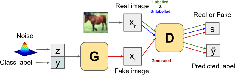
Figure 1: Base model: Semi-ACGAN. D learns from the labelled (green arrow), the unlabelled (blue arrow) samples as well as the generated (red arrow) samples. D predicts both the source (real or fake) and the class label for the labelled and generated samples, whereas, for the unlabelled samples, D only predicts the source.

2.3 Base Model: Semi-ACGAN

The base network is a modified auxiliary classifier GAN (Semi-ACGAN) and, thus, consists of a generator G, a discriminator D with an auxiliary classifier. We denote the weights of the base network for task $k$ using $\mathbf{\Theta}_{k}$.

In Semi-ACGAN, G is conditioned on the class label $\boldsymbol{y}$ along with the noise $\boldsymbol{z}_{b}$. Thus, the generated samples $x_{\text{fake}}=\text{G}(\boldsymbol{z}_{b},\boldsymbol{y})$ correspond to a class label. Let $\boldsymbol{s}$ denote whether the source of the sample $\boldsymbol{x}$ is real or fake. For a sample $\boldsymbol{x}$, the discriminator gives the probability distribution over the sources $p(\boldsymbol{s}|\boldsymbol{x})$ as well as the probability distribution over the classes $p(\boldsymbol{y}|\boldsymbol{x})$, i.e., $[p(\boldsymbol{s}|\boldsymbol{x}),p(\boldsymbol{y}|\boldsymbol{x})]=\text{D}(\boldsymbol{x})$.

Let us denote the real sample using $\boldsymbol{x}_{\text{real}}$ and the actual class of the sample using $\hat{\boldsymbol{y}}$. The training objective consists of the following:

(i) For Labelled data:

a. Log likelihood of the correct source,

$$\mathcal{L}_{s}^{\text{L}}=\mathop{\mathbb{E}}[\log p(\boldsymbol{s}= \text{real}|\boldsymbol{x}_{\text{real}})]+$$

$$\mathop{\mathbb{E}}[\log p(\boldsymbol{s}=\text{fake}|\boldsymbol{x}_{\text{fake}})]$$ (1)

b. Log likelihood of the correct class,

$$\mathcal{L}_{c}^{\text{L}}=\mathop{\mathbb{E}}[\log p(\boldsymbol{y}= \hat{\boldsymbol{y}}|\boldsymbol{x}_{\text{real}})]+$$

$$\mathop{\mathbb{E}}[\log p(\boldsymbol{y}=\hat{\boldsymbol{y}}|\boldsymbol{x}_{\text{fake}})]$$ (2)

(ii) For Unlabelled data:

a. Log likelihood of the correct source for real images,

$$\mathcal{L}_{s}^{\text{U}}=\mathop{\mathbb{E}}[\log p(\boldsymbol{s}= \text{real}|\boldsymbol{x}_{\text{real}})]$$ (3)

The discriminator D learns by maximizing $\mathcal{L}_{c}^{\text{L}}+\mathcal{L}_{s}^{\text{L}}+\mathcal{L}_{s}^{\text{U}}$, whereas the generator G learns by maximizing $\mathcal{L}_{c}^{\text{L}}-\mathcal{L}_{s}^{\text{L}}$.

Note that since the class information of unlabelled data is missing, we do not consider the log-likelihood of the correct class in the case of unlabelled data.

The generator G is a neural network that takes both the class label and noise. The class label embedding is obtained from the class id using a class embedding layer that is trainable. Thus, G learns to generate class-specific samples.

The discriminator D is a neural network with shared layers and two separate output layers: i. validity layer: output layer for correct source, ii. auxiliary classifier layer: output layer for correct class label. D utilizes only the validity layer for unlabelled data while using both the validity and auxiliary classifier layers for labelled data. Since the class information is known for the generated images, both the output layers of D are used for generated images.

The shared layers of D enable learning from both the labelled and the unlabelled data. As the training progresses, G learns to generate realistic samples with known class labels, enabling D to do better classification.

Figure 1 shows the modules of the base network Semi-ACGAN. As the real samples can consist of both the labelled data and unlabelled data, the figure shows it using green and blue arrows, respectively. On the other hand, the red arrows depict the generated samples. Moreover, the outputs are colour coded similarly.

2.4 Task-specific Parameter Distribution: Hypernetwork

As $B$ instances of the trained base network are used as the inputs for training the hypernetwork, we denote this set using $\{\mathbf{\Theta}_{k}^{l}\}_{l=1}^{B}$ for task $k$. Since a VAE-like model having task-specific conditional prior is used as the hypernetwork, we define the parameters of the hypernetwork as $[\boldsymbol{\theta},\boldsymbol{\phi}]$ such that $\boldsymbol{\theta}$ and $\boldsymbol{\phi}$ are the encoder and decoder parameters of the hypernetwork respectively.

The hypernetwork VAE models the task-specific parameter distribution $p(\mathbf{\Theta}|\boldsymbol{t})$. Thus, learning the hypernetwork enables the consolidation of knowledge from the previous tasks in the meta-space. The vector representation $\boldsymbol{t}_{j}$ for the $k^{th}$ task can be any fixed-length vector representation including Word2Vec Mikolov et al. (2013), GloVe Pennington et al. (2014) or just a one-hot encoding of the task identity. We use $\boldsymbol{t}$ to denote $\boldsymbol{t}_{j}$ in this subsection for brevity.

Inspired from MERLIN Joseph and Balasubramanian (2020), the hypernetwork is trained by optimizing a VAE-like objective Kingma and Welling (2013). The computation of the marginal likelihood of the parameter distribution $p_{\boldsymbol{\theta}}(\mathbf{\Theta}|\boldsymbol{t})=\int p_{\boldsymbol{\theta}}(\mathbf{\Theta}|\boldsymbol{z},\boldsymbol{t})p_{\boldsymbol{\theta}}(\boldsymbol{z}|\boldsymbol{t})d\boldsymbol{z}$ is intractable because of the intractability in the computation of its true posterior $p_{\boldsymbol{\theta}}(\boldsymbol{z}|\mathbf{\Theta},\boldsymbol{t})=\frac{p_{\boldsymbol{\theta}}(\mathbf{\Theta}|\boldsymbol{z},\boldsymbol{t})p_{\boldsymbol{\theta}}(\boldsymbol{z}|\boldsymbol{t})}{p_{\boldsymbol{\theta}}(\mathbf{\Theta}|\boldsymbol{t})}$. Thus, we introduce an approximate variational posterior $q_{\boldsymbol{\phi}}(\boldsymbol{z}|\mathbf{\Theta},\boldsymbol{t})$ to resolve the problem of intractibility. The log marginal likelihood can be written as:

$$p_{\boldsymbol{\theta}}(\mathbf{\Theta}|\boldsymbol{t})=KL(q_{\boldsymbol{\phi}}(\boldsymbol{z}|\mathbf{\Theta},\boldsymbol{t})~{}\|~{}p_{\boldsymbol{\theta}} (\boldsymbol{z}|\mathbf{\Theta},\boldsymbol{t}))~{}~{}+$$

$$\mathcal{L}(\boldsymbol{\theta},\boldsymbol{\phi}|\mathbf{\Theta},\boldsymbol{t})$$ (4)

where $\mathcal{L}(\boldsymbol{\theta},\boldsymbol{\phi}|\mathbf{\Theta},\boldsymbol{t})=\int_{\boldsymbol{z}}q_{\boldsymbol{\phi}}(\boldsymbol{z}|\mathbf{\Theta},\boldsymbol{t})\log\frac{p_{\boldsymbol{\theta}}(\boldsymbol{z},\mathbf{\Theta}|\boldsymbol{t})}{q_{\boldsymbol{\phi}}(\boldsymbol{z}|\mathbf{\Theta},\boldsymbol{t})}$ is the evidence lower bound (ELBO). This lower bound can be maximized in order to maximize the log-likelihood.

Further, $\mathcal{L}(\boldsymbol{\theta},\boldsymbol{\phi}|\mathbf{\Theta},\boldsymbol{t})$ can be expressed as (refer to Joseph and Balasubramanian (2020) for complete derivation):

$$\mathcal{L}(\boldsymbol{\theta},\boldsymbol{\phi}|\mathbf{\Theta},\boldsymbol{t})=-KL(q_{\boldsymbol{\phi}} (\boldsymbol{z}|\mathbf{\Theta},\boldsymbol{t})~{}\|~{}p_{\boldsymbol{\theta}}(\boldsymbol{z}|\boldsymbol{t}))~{}~{}+$$

$$\mathop{\mathbb{E}}_{q_{\boldsymbol{\phi}}(\boldsymbol{z}|\mathbf{\Theta},\boldsymbol{t})}[\log p_{\boldsymbol{\theta}}(\mathbf{\Theta}|\boldsymbol{z},\boldsymbol{t})]$$ (5)

Maximizing Eqn. 5 minimizes the KL divergence term, causing the approximate posterior weights to become close to the task-specific prior $p_{\boldsymbol{\theta}}(\boldsymbol{z}|\boldsymbol{t})$. The second term is the expected negative reconstruction error, and it requires sampling to estimate. The hypernetwork parameters $\boldsymbol{\phi}$ and $\boldsymbol{\theta}$, also known as encoder and decoder parameters, are trained using backpropagation and stochastic gradient descent. We assume that $p_{\boldsymbol{\theta}}(.)$ and $q_{\boldsymbol{\phi}}(.)$ are Gaussian distributions. Moreover, the reparameterization trick Kingma and Welling (2013) is used to backpropagate through the stochastic parameters. Taking $\{\mathbf{\Theta}_{k}^{l}\}_{l=1}^{B}$ as the input, we train the hypernetwork by maximizing Eqn. 5.

Unlike standard VAE, the task-specific prior is not an isotropic multivariate Gaussian. It is given by:

$$p_{\boldsymbol{\theta}}(\boldsymbol{z}|\boldsymbol{t})=\mathcal{N}(\boldsymbol{z}|\boldsymbol{\mu_{\boldsymbol{t}}},\boldsymbol{\Sigma_{\boldsymbol{t}}})$$ (6)

where $\boldsymbol{\mu_{\boldsymbol{t}}}=\boldsymbol{W}_{\boldsymbol{\mu}}^{T}\boldsymbol{t}$ and $\boldsymbol{\Sigma_{\boldsymbol{t}}}=\boldsymbol{W}_{\boldsymbol{\Sigma}}^{T}\boldsymbol{t}$ such that $\boldsymbol{W}_{\boldsymbol{\mu}}$ and $\boldsymbol{W}_{\boldsymbol{\Sigma}}$ are trainable parameters, and learned along with the hypernetwork parameters.

2.5 Meta-Consolidation

Training the VAE directly on $\{\mathbf{\Theta}_{k}^{l}\}_{l=1}^{B}$ causes a distributional shift, i.e., a bias towards the current task $k$. So, the hypernetwork VAE needs to consolidate the knowledge from the previous tasks. We call this meta-consolidation. We store the means and covariances of all the learned task-specific prior, which adds a negligible storage complexity. The meta-consolidation mechanism is described below:

1. For each task $\mathcal{T}_{j}$ till current task $k$ ($j={1,\cdots,k}$),

   1. Sample $\boldsymbol{z_{t_{j}}}$ from task-specific prior:

      $$\boldsymbol{z_{t_{j}}}\sim\mathcal{N}(\boldsymbol{z}|\boldsymbol{\mu_{\boldsymbol{t_{j}}}},\boldsymbol{\Sigma_{\boldsymbol{t_{j}}}})$$

   2. Sample $P$ many semi-supervised base pseudo-models from decoder:

      $$\mathbf{\Theta}_{j}^{i}\sim p_{\boldsymbol{\theta}}(\mathbf{\Theta}|\boldsymbol{z_{t_{j}}},\boldsymbol{t}_{j});~{}\text{where}~{}i\in\{1,2,\cdots,P\}$$

   3. Compute the loss using Eqn. 5:

      $$Loss=\sum_{i=1}^{P}\mathcal{L}(\boldsymbol{\theta},\boldsymbol{\phi}|\mathbf{\Theta}_{j}^{i},\boldsymbol{t}_{j})$$

   4. Optimize $Loss$ to update parameters $\boldsymbol{\phi}$, $\boldsymbol{\theta}$

2.6 Inference

Learning the task-specific parameter distribution $p_{\boldsymbol{\theta}}(\mathbf{\Theta}|\boldsymbol{z},\boldsymbol{t})$ gives the ability to sample multiple $\mathbf{\Theta}$’s during inference. This ability provides an ensembling effect of multiple models without storing the models a priori. Like most of the other continual learning approaches, we use a small exemplar memory buffer $\mathcal{E}$ for fine-tuning during inference.

Our approach can work with or without task-specific information during inference. However, we focus on the task-agnostic setting as it is more realistic and challenging. The inference procedure for task-agnostic inference is described below:

1. Aggregate the stored means and covariances:

   $$\boldsymbol{\mu}=\frac{1}{k}\sum_{i=1}^{k}\boldsymbol{\mu}_{t_{i}},\boldsymbol{\Sigma}=\frac{1}{k}\sum_{i=1}^{k}\boldsymbol{\Sigma}_{t_{i}}$$

2. Sample $\boldsymbol{z}$ from prior with aggregated mean and covariance:

   $$\boldsymbol{z}\sim\mathcal{N}(\boldsymbol{z}|\boldsymbol{\mu},\boldsymbol{\Sigma})$$

3. Sample $E$ number of $\mathbf{\Theta}$’s (semi-supervised base models) from learned decoder:

   $$\mathbf{\Theta}^{i}\sim p_{\boldsymbol{\theta}}(\mathbf{\Theta}|\boldsymbol{z});~{}\text{where}~{}i\in\{1,2,\cdots,E\}$$

4. Fine-tune $\{\mathbf{\Theta}^{i}\}_{i=1}^{E}$ on $\mathcal{E}$

5. Ensemble results from $\{\mathbf{\Theta}^{i}\}_{i=1}^{E}$ and solve tasks $\{{\mathcal{T}_{i}}\}_{i=1}^{k}$

The inference procedure for task-aware inference is given as below:

1. For each task $\mathcal{T}_{j};$ $j\in\{1,\cdots,k\}$

   1. Sample $\boldsymbol{z_{t_{j}}}$ from task-specific prior:

      $$\boldsymbol{z_{t_{j}}}\sim\mathcal{N}(\boldsymbol{z}|\boldsymbol{\mu_{t_{j}}},\boldsymbol{\Sigma_{t_{j}}})$$

   2. Sample $E$ number of $\mathbf{\Theta}$’s from learned decoder:

      $$\mathbf{\Theta}_{j}^{i}\sim p_{\boldsymbol{\theta}}(\mathbf{\Theta}|\boldsymbol{z_{t_{j}}},\boldsymbol{t_{j}});~{}\text{where}~{}i\in\{1,2,\cdots,E\}$$

   3. Fine-tune $\{\mathbf{\Theta}_{j}^{i}\}_{i=1}^{E}$ on $\mathcal{E}$

   4. Ensemble results from $\{\mathbf{\Theta}_{j}^{i}\}_{i=1}^{E}$ and solve task $\mathcal{T}_{j}$

Labelled data$\rightarrow$	500 (120)		250 (60)		100 (24)		50 (12)
Methods$\downarrow$	$\boldsymbol{A\uparrow}$	$\boldsymbol{F\downarrow}$	$\boldsymbol{A\uparrow}$	$\boldsymbol{F\downarrow}$	$\boldsymbol{A\uparrow}$	$\boldsymbol{F\downarrow}$	$\boldsymbol{A\uparrow}$	$\boldsymbol{F\downarrow}$
Single-SSL	59.57	2.90	59.80	3.44	57.35	1.87	54.38	0.72
EWC-SSL	60.11	0.88	60.89	3.20	60.78	3.17	59.65	2.23
MCSSL (Ours)	63.72	-4.61	63.55	2.45	63.37	3.60	63.00	11.25

Table 1: Average accuracy ($A$) ($\uparrow$ higher is better) and average forgetting ($F$) ($\downarrow$ lower is better) of MCSSL and the baseline approaches modified to use both labelled and unlabelled data on Semi-Split CIFAR-10 dataset. The number of labelled data is varied, whereas, the number of unlabelled data is fixed to 1000 (240). The number inside () denotes the labelled memory buffer size.

Labelled data$\rightarrow$	500 (120)		250 (60)		100 (24)		50 (12)
Methods$\downarrow$	$\boldsymbol{A\uparrow}$	$\boldsymbol{F\downarrow}$	$\boldsymbol{A\uparrow}$	$\boldsymbol{F\downarrow}$	$\boldsymbol{A\uparrow}$	$\boldsymbol{F\downarrow}$	$\boldsymbol{A\uparrow}$	$\boldsymbol{F\downarrow}$
Single	63.48	10.81	59.54	1.81	53.65	-3.76	51.68	3.57
EWC	67.32	5.20	59.25	10.01	52.82	-0.39	49.82	0.04
MERLIN	59.71	0.51	33.77	-0.48	22.71	2.07	17.84	1.06
MCSSL (Ours)	63.72	-4.61	63.55	2.45	63.37	3.60	63.00	11.25

Table 2: Average accuracy ($A$) ($\uparrow$ higher is better) and average forgetting ($F$) ($\downarrow$ lower is better) upon varying the number of labelled data on Semi-Split CIFAR-10 dataset. The number inside () denotes the labelled memory buffer size. MCSSL (Ours) uses some unlabelled data, whereas other baseline models only use the labelled data.

3 Related Work

Most of the existing continual learning approaches focus on the problem of continual supervised learning. These approaches consolidate knowledge either in the weight space, data space or meta-space.

Elastic Weight Consolidation (EWC) Kirkpatrick et al. (2017) is a regularization based approach that penalizes drastic changes in the parameters that have a large influence on prediction. Variational Continual Learning (VCL) Nguyen et al. (2018) is a probabilistic regularization based approach using Bayesian neural networks. They treat the posterior of the current task as the prior for the next task as it naturally emerges from online variational inference. Learning without Forgetting (LwF) Li and Hoiem (2018) uses knowledge distillation to preserve the knowledge of previous tasks.

Gradient Episodic Memory (GEM) Lopez-Paz and Ranzato (2017) stores a limited number of samples to retrain while constraining new task updates to not interfere with knowledge of previous tasks. Aljundi et al. (2019) extended this idea by selecting subsets of samples that approximate the region of the data seen in the previous tasks.

von Oswald et al. (2019) operates in the meta-space as it learns a hypernetwork that generates the weights of the base model. However, they learn a task identity conditioned deterministic function. Similarly, recent work by Joseph and Balasubramanian (2020) consolidates the knowledge from previous tasks in the meta-space of weight generating hypernetwork. They learn the task-specific distribution of weights, giving them the ability to ensemble during prediction.

Some recent approaches focus on the problem of continual unsupervised learning. Rao et al. (2019) presents an approach for unsupervised representation learning with a dynamic expansion based approach using a latent mixture-of-Gaussians. Lee et al. (2019) focuses on the discriminative and generative tasks using Dirichlet process mixture models for dynamic expansion with a generative process different from Rao et al. (2019).

A recent approach, named, DistillMatch Smith et al. (2021) tries to address the problem of Continual Semi-Supervised Learning. However, the unlabeled data in continual tasks significantly differ from our set-up, as Smith et al. (2021) uses the super-class structure of the CIFAR dataset. DistillMatch combines pseudo-labelling for semi-supervised learning, knowledge distillation for continual learning, along with consistency regularization as it uses FixMatch Sohn et al. (2020) as the base semi-supervised learner. Moreover, it has an out-of-distribution detection scheme required due to its problem set-up. However, unlike our approach, DistillMatch is not a generative approach, and thus, the distribution of input is not directly modeled.

4 Experiments

We propose a novel dataset for continual semi-supervised learning. We conduct a comprehensive analysis of our proposed model MCSSL on the proposed modified CIFAR dataset and compare our model with other state-of-the-art approaches. We describe the dataset details, evaluation metrics, hyperparameter settings, experimental results and analysis in this section. All the results are shown for task-agnostic setting as it is more realistic and challenging.

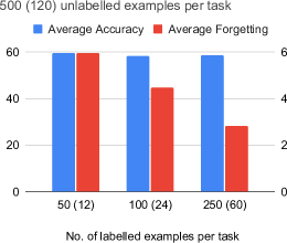
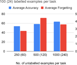
Figure 2: Top: Semi-Split CIFAR-10 dataset with varying number of labelled data, and fixed number of unlabelled data. Bottom: Semi-Split CIFAR-10 dataset with varying number of unlabelled data, and fixed number of labelled data. The number inside () denotes memory buffer size.

4.1 Dataset Details

We experiment with the CIFAR dataset in a continual learning semi-supervised set-up. Split CIFAR-10 Zenke et al. (2017) dataset is a supervised continual learning benchmark dataset that has 10 tasks with 45,000 images in total such that each task contains 2 classes. We modify Split CIFAR-10 dataset for continual semi-supervised learning set-up. Thus, we have 10 tasks in total where each task contains 2 classes with a varying number of labelled data and unlabelled data. We name this modified dataset as Semi-Split CIFAR-10.

4.2 Training Details and Hyperparameters

The base model Semi-ACGAN uses convolutional deep neural networks for G and D. The validity and auxiliary classifier layers of D are both linear layers with sigmoid and softmax functions applied respectively to get the scores. During training, number of base models is 5, and for training these base models, we use Adam optimizer with initial learning rate of 0.0002. We provide the architecture details of G and D below.

Detailed architecture of G: [BatchNorm; Upsampling: scale=4; Conv: 3x3, 16 filters, stride=1, padding=1); BatchNorm; LeakyReLU; Conv: 3x3, 3 filters, stride=1, padding=1); Tanh].

Detailed architecture of shared layers of D: [Conv: 3x3, 16 filters, stride=2, padding=1; LeakyReLU; Dropout: p=0.25; Conv: 3x3, 32 filters, stride=2, padding=1; LeakyReLU; Dropout: p=0.25; BatchNorm].

The hypernetwork uses 5 base models to learn its encoder and decoder parameters. The chunking trick proposed by von Oswald et al. (2019) is used to keep the size of the VAE small. The weights of the base models are flattened and then split into chunks of size 250. We train the hypernetwork conditioned on the chunks, and the chunk embeddings are learned together with the hypernetwork parameters. The weights are assembled back for making the inference. We use the one-hot encoding of the task identity.

In the hypernetwork VAE, the encoder network has one fully connected layer with 30 neurons. Moreover, the decoder network architecture is a mirror of the encoder network architecture. This is followed by two layers for predicting mean and diagonal covariance vectors respectively. The dimension of latent $\boldsymbol{z}$ is 10. The hypernetwork VAE is trained for 5 epochs using Adadelta optimizer with an initial learning rate of 0.005 and batch size of 1.

During inference, we sample 15 models from the decoder for ensembling using majority voting. Further, the labelled and unlabelled data in the memory buffer are used to fine-tune the models. Since the base models are loaded sequentially at a time (saving only the final logits) not more than one model is ever loaded in the memory at one time.

4.3 Evaluation Metrics

We define $a_{k,j}$ as the accuracy on the test set of $j^{th}$ task, after model is trained on $k^{th}$ task. Following previous works on continual learning, we use the metrics given below to evaluate the models:

1. Average Accuracy:

   $$A=\frac{1}{K}\sum_{k=1}^{K}A_{k}~{};\text{ where }A_{k}=\frac{1}{k}\sum_{j=1}^{k}a_{k,j}$$

2. Average Forgetting:

   $$F=\frac{1}{K}\sum_{k=1}^{K}F_{k}~{};$$

   $$\text{ where }F_{k} =\frac{1}{k-1}\sum_{j=1}^{k-1}\max_{l\in\{1,\cdots,k-1\}}(a_{l,j}-a_{k,j})$$

4.4 Results and Analysis

We adapt EWC for continual semi-supervised setting, denoted as EWC-SSL, and conduct experiments with a varying number of labelled data. We also train a single base model Semi-ACGAN without any continual learning mechanism and denote it using Single-SSL. The labelled data is used during continual training, and a small fraction of it is stored in a memory buffer for fine-tuning during inference. Table 1 shows the results on Semi-Split CIFAR-10 dataset. We compare our approach with Single-SSL and EWC-SSL as baseline continual semi-supervised approaches. We fix number of unlabelled data to 1000 per task with unlabelled data memory buffer size of 240 per task for all the models. The decrease in number of labelled data does not have much significant impact on the performance of MCSSL as it consistently outperforms baseline approaches in all settings. This suggests that our approach generalises better in low data regimes.

In order to demonstrate the ability of our model to leverage unlabeled data, we also compare with other continual supervised baseline approaches in Table 2. Here, Single denotes a Resnet18 classifier trained without any continual learning mechanism. EWC also uses a Resnet18 classifier, whereas MERLIN uses a modified Resnet18 classifier as described in Joseph and Balasubramanian (2020). Our model uses labelled data along with some unlabelled data, whereas other models use only labelled data. As our model outperforms other approaches in most settings, we observe that it does better than others as labelled data decreases. Decreasing labelled data has no significant effect on our model, whereas the performance of other models drops drastically.

In Fig. 2 (Top), we fix the number of unlabelled examples per task as 500 with 120 unlabelled samples in the memory buffer for fine-tuning as we vary the number of labelled examples per task. We notice that the accuracy slightly increases with an increase in the labelled data. Here, forgetting tends to decrease as the labelled examples per task increases.

Fig. 2 (Bottom) shows a varying number of unlabelled examples upon fixing the number of labelled examples per task as 100 with 24 labelled examples in the memory buffer for fine-tuning. We observe that upon fixing the number of labelled data per task, the accuracy increases with an increase in unlabelled data. Also, forgetting tends to increase as the examples per task increases, but it is not significant.

5 Conclusion

We proposed a novel continual semi-supervised learning scheme in which tasks with both unlabeled and labelled examples arrive sequentially. We developed a task-specific weight generation-based approach for continual semi-supervised learning problem. We utilize a semi-supervised auxiliary classifier GAN (Semi-ACGAN) as the base model. We also extended other continual learning approaches to use both labelled and unlabelled data, and comparisons show that MCSSL performs better on the Semi-Split CIFAR-10 dataset in most of the settings. We also outperform other continual supervised baseline approaches that show the ability of our model MCSSL to leverage knowledge from the unlabelled examples. Moreover, MCSSL performs well even for a low number of labelled examples. In future work, we plan to evaluate MCSSL on more benchmarks and baselines.

Acknowledgments: This work was supported by Qualcomm Innovation Fellowship.

References

- Aljundi et al. [2019] Rahaf Aljundi, Min Lin, Baptiste Goujaud, and Yoshua Bengio. Gradient based sample selection for online continual learning. In NeurIPS, 2019.
- Alvarez and Squire [1994] Pablo Alvarez and Larry R Squire. Memory consolidation and the medial temporal lobe: a simple network model. PNAS, 91(15), 1994.
- Caramazza and Mahon [2003] Alfonso Caramazza and Bradford Z Mahon. The organization of conceptual knowledge: the evidence from category-specific semantic deficits. Trends in cognitive sciences, 7(8), 2003.
- Caramazza and Shelton [1998] Alfonso Caramazza and Jennifer R Shelton. Domain-specific knowledge systems in the brain: The animate-inanimate distinction. Journal of cognitive neuroscience, 10(1), 1998.
- Chaudhry et al. [2019] Arslan Chaudhry, Marc’Aurelio Ranzato, Marcus Rohrbach, and Mohamed Elhoseiny. Efficient lifelong learning with a-gem. In ICLR, 2019.
- Handjaras et al. [2016] Giacomo Handjaras, Emiliano Ricciardi, Andrea Leo, Alessandro Lenci, Luca Cecchetti, Mirco Cosottini, Giovanna Marotta, and Pietro Pietrini. How concepts are encoded in the human brain: a modality independent, category-based cortical organization of semantic knowledge. Neuroimage, 135, 2016.
- Joseph and Balasubramanian [2020] KJ Joseph and Vineeth N Balasubramanian. Meta-consolidation for continual learning. arXiv preprint arXiv:2010.00352, 2020.
- Kingma and Welling [2013] Diederik P Kingma and Max Welling. Auto-encoding variational bayes. arXiv preprint arXiv:1312.6114, 2013.
- Kirkpatrick et al. [2017] James Kirkpatrick, Razvan Pascanu, Neil Rabinowitz, Joel Veness, Guillaume Desjardins, Andrei A Rusu, Kieran Milan, John Quan, Tiago Ramalho, Agnieszka Grabska-Barwinska, et al. Overcoming catastrophic forgetting in neural networks. Proceedings of the national academy of sciences, 114(13), 2017.
- Lee et al. [2019] Soochan Lee, Junsoo Ha, Dongsu Zhang, and Gunhee Kim. A neural dirichlet process mixture model for task-free continual learning. In ICLR, 2019.
- Li and Hoiem [2018] Zhizhong Li and Derek Hoiem. Learning without forgetting. IEEE TPAMI, 40(12), 2018.
- Lopez-Paz and Ranzato [2017] David Lopez-Paz and Marc’Aurelio Ranzato. Gradient episodic memory for continual learning. In NeurIPS, 2017.
- Mahon et al. [2009] Bradford Z Mahon, Stefano Anzellotti, Jens Schwarzbach, Massimiliano Zampini, and Alfonso Caramazza. Category-specific organization in the human brain does not require visual experience. Neuron, 63(3), 2009.
- Mikolov et al. [2013] Tomas Mikolov, Ilya Sutskever, Kai Chen, Greg Corrado, and Jeffrey Dean. Distributed representations of words and phrases and their compositionality. NeurIPS, 2013.
- Nguyen et al. [2018] Cuong V Nguyen, Yingzhen Li, Thang D Bui, and Richard E Turner. Variational continual learning. In ICLR, 2018.
- Odena et al. [2017] Augustus Odena, Christopher Olah, and Jonathon Shlens. Conditional image synthesis with auxiliary classifier gans. In International conference on machine learning. PMLR, 2017.
- Pennington et al. [2014] Jeffrey Pennington, Richard Socher, and Christopher D Manning. Glove: Global vectors for word representation. In EMNLP, 2014.
- Rao et al. [2019] Dushyant Rao, Francesco Visin, Andrei Rusu, Razvan Pascanu, Yee Whye Teh, and Raia Hadsell. Continual unsupervised representation learning. NeurIPS, 32, 2019.
- Rebuffi et al. [2017] Sylvestre-Alvise Rebuffi, Alexander Kolesnikov, Georg Sperl, and Christoph H Lampert. icarl: Incremental classifier and representation learning. In CVPR. IEEE, 2017.
- Rolnick et al. [2019] David Rolnick, Arun Ahuja, Jonathan Schwarz, Timothy Lillicrap, and Gregory Wayne. Experience replay for continual learning. In NeurIPS, 2019.
- Salimans et al. [2016] Tim Salimans, Ian J Goodfellow, Wojciech Zaremba, Vicki Cheung, Alec Radford, and Xi Chen. Improved techniques for training gans. In NeurIPS, 2016.
- Shin et al. [2017] Hanul Shin, Jung Kwon Lee, Jaehong Kim, and Jiwon Kim. Continual learning with deep generative replay. In NeurIPS, 2017.
- Smith et al. [2021] James Smith, Jonathan Balloch, Yen-Chang Hsu, and Zsolt Kira. Memory-efficient semi-supervised continual learning: The world is its own replay buffer. arXiv preprint arXiv:2101.09536, 2021.
- Sohn et al. [2020] Kihyuk Sohn, David Berthelot, Nicholas Carlini, Zizhao Zhang, Han Zhang, Colin A Raffel, Ekin Dogus Cubuk, Alexey Kurakin, and Chun-Liang Li. Fixmatch: Simplifying semi-supervised learning with consistency and confidence. NeurIPS, 33, 2020.
- von Oswald et al. [2019] Johannes von Oswald, Christian Henning, João Sacramento, and Benjamin F Grewe. Continual learning with hypernetworks. In ICLR, 2019.
- Wilson and McNaughton [1994] Matthew A Wilson and Bruce L McNaughton. Reactivation of hippocampal ensemble memories during sleep. Science, 265(5172), 1994.
- Zenke et al. [2017] Friedemann Zenke, Ben Poole, and Surya Ganguli. Continual learning through synaptic intelligence. In ICML. JMLR. org, 2017.