Multilevel orthogonal Bochner function subspaces with applications to robust machine learning

Abstract.

In our approach, we consider the data as instances of a random field within a relevant Bochner space. Our key observation is that the classes can predominantly reside in two distinct subspaces. To uncover the separation between these classes, we employ the Karhunen-Loève expansion and construct the appropriate subspaces. This allows us to effectively reveal the distinction between the classes. The novel features forming the above bases are constructed by applying a coordinate transformation based on the recent Functional Data Analysis theory for anomaly detection. The associated signal decomposition is an exact hierarchical tensor product expansion with known optimality properties for approximating stochastic processes (random fields) with finite dimensional function spaces. Using a hierarchical finite dimensional expansion of the nominal class, a series of orthogonal nested subspaces is constructed for detecting anomalous signal components. Projection coefficients of input data in these subspaces are then used to train a Machine Learning (ML classifier. However, due to the split of the signal into nominal and anomalous projection components, clearer separation surfaces for the classes arise. In fact we show that with a sufficiently accurate estimation of the covariance structure of the nominal class, a sharp classification can be obtained. This is particularly advantageous for large unbalanced datasets. We demonstrate it on a number of high-dimensional datasets. This approach yields significant increases in accuracy of ML methods compared to using the same ML algorithm with the original feature data. Our tests on the Alzheimer’s Disease ADNI dataset shows a dramatic increase in accuracy (from 48% to 89% accuracy). Furthermore, tests using unbalanced semi-synthetic datasets created from the benchmark GCM dataset confirm increased accuracy as the dataset becomes more unbalanced.

1. Introduction

We introduce a systematic approach for the construction of machine learning (ML) feature vectors that improves class separations, using techniques in probability theory and functional (data) analysis. Our implementations involve techniques from computational applied mathematics and computer science. We apply the approach within a framework of high dimensional noisy gene expression data for cancer diagnostics; this leads to significant increases in predictive accuracy. Furthermore we apply it to the well-known ADNI Alzheimer Disease dataset [19]. Due to its foundation in functional analysis and tensor product expansions, this approach can be easily extended to classification problems on complex topologies, including gene expression networks.

We treat the data as realizations of a random field in a suitable Bochner space. The key insight of our approach is to realize that the classes can be localized to two separate subspaces in a Bochner function space. By exploiting the Karhunen-Loève expansion, these subspaces can be constructed to reveal an optimal class separation (See Figure 1). This paper is a novel application of the theory developed in [3]. In particular, we show how functional data analysis [12, 13] can be applied to statistical machine learning. The problem of classification in machine learning has been studied and benchmarked for decades, and this method provides an entirely new way of approaching the problem with a new feature map that is based on novel estimates of the underlying covariance structure, applied to quantitative anomaly calibrations as novel ML features. This approach effectively augments current ML algorithms.

A fundamental issue in ML predictive modeling is robustness and sensitivity to data quality. Machine learning with complex noisy observations involves a host of difficulties including the problem of overfitting, which can give rise to highly unstable and inaccurate decision boundaries. This problem is particularly difficult for data with high dimension ($p$) and low sample size ($N$), ( i.e. $p\gg N$ ), for example gene expression arrays, in which genes number in the tens of thousands while available tissue samples are limited by high biopsy costs. However, the problem can also present itself in high dimension with even larger large sample sizes (i.e. $p\ll N$), and noisy inputs again leading to unstable decision boundary oscillations. Such oscillations generally arise from overfitting noise, and can lead to poor machine performance.

In Figure 1 (a), (b), (c) an illustrative example of such classification is shown. For (a) we have that our data is well separated with the blue dots representing the first class and the orange dots the second. Due to the separation of the data it is in principle easy to construct a decision boundary. In (b) the data classes are mixed. Furthermore the data can be noisy and diffusive in high dimensions, leading to unstable boundary decision surfaces. The fundamental questions are: Does there exist a good separation of the data classes in some coordinate system? How do we construct a transformation that can reveal this separation in an appropriate space (See Figure 1 (c))? To answer these questions we treat the data as realizations of a random field.

Our overarching goals in this work are to: i) To develop stochastic functional (data) analysis approaches for significantly improving accuracy and robustness of machine learning methods on high dimensional noisy datasets that can also be based on complex topologies; ii) To motivate and develop high performance computing algorithms based on these approaches.

Figure 1. Illustrative example of binary classification with blue and orange dots. For (a) we have that our data are well separated, with blue dots representing the first class and orange dots the second. Due to the separation of the data it is in principle easy to construct a decision boundary. (b) For this case the data classes are mixed, leading to complex boundary decision surfaces that are hard to build, yielding low accuracy. Furthermore the data can be noisy and diffusive in high dimensions, leading to unstable boundary decision surfaces. (c) After applying an appropriate transformation using the stochastic coordinate transformations developed in this paper the classes separate, leading to stable boundary decision surfaces.

The related signal decomposition is an exact hierarchical tensor product expansion with known optimality properties for approximating stochastic processes (random fields) with finite dimensional function spaces as ranges. In principle these primary low dimensional range spaces can capture most of the stochastic behavior of ‘underlying signals in a given nominal class, and can reject signals in alternative classes as stochastic anomalies. Using a hierarchical finite dimensional KL expansion for the nominal class, a series of orthogonal nested subspaces is constructed for detecting anomalous signal components relative to this nominal class. Projection coefficients of input data in these subspaces are then used to train a Machine Learning (ML) classifier. However, due to the split of the signal into nominal and anomalous projection components, clearer separation surfaces of the classes arise. In fact we show that with a sufficiently accurate estimation of the covariance structure of the nominal class, a sharp classification can be obtained. This is particularly advantageous when large unbalanced datasets are available.

We have carefully formulated this concept and demonstrated it on a number of high-dimensional datasets in cancer diagnostics. This approach yields significant increases in accuracy over ML methods that use standard original feature data. In particular, this method leads to a significant increase in precision and accuracy for the Alzheimer’s Disease ADNI dataset (from 48% to 89% accuracy for the Support Vector Machine (SVM) with a radial kernel, in the transformed space). Furthermore, tests on complex unbalanced semi-synthetic data show that increases in available data dramatically improve accuracy. Tests from unbalanced semi-synthetic datasets created from the GCM dataset confirmed large increases in accuracy as the dataset becomes more unbalanced.

Highly unbalanced datasets are a difficult problem for machine learning algorithms. There are many approaches to compensate for an unbalanced dataset. This may involve, for example, removing the unbalanced portion of the data, bootstrapping to create more samples of the smaller class of data, or adjusting the ML algorithm by using weights [23]. However, many of these solutions are unsatisfactory. In particular, if the number of samples of the smaller class is very small and/or are noisy. This has motivated the development of one class semi-supervised methods. See [18] for a comprehensive survey of these methods. The Multilevel Orthogonal Subspace (MOS) KL approach developed in our paper solves this problem in a more elegant form. Furthermore, as the dataset becomes more unbalanced the accuracy increases.

2. Mathematical preliminaries

We demonstrate our approach to the ML classification problem. A novel strategy for classification will here be the construction of a series of subspaces orthogonal to a stochastic representation of data belonging to one of the classes. For two class classification, the second class is treated as a change or anomaly with respect to the first. The constructed subspaces allow detection of such ‘anomalies’ with high accuracy from data and projection coefficients, and are used to train an ML classifier.

More precisely, the variation of the data is viewed as a realization of a random field; the Karhunen Loève expansion is an important tool for representing such fields as spatial-stochastic tensor expansions. This optimal decomposition is well suited for the analysis of such random fields. Let $(\Omega,\mathcal{F},\mathbb{P})$ be a complete probability space, with $\Omega$ a set of outcomes, and $\mathcal{F}$ a $\sigma$-algebra of events equipped with the probability measure $\mathbb{P}$. Let $U$ be a domain of $\mathbb{R}^{d}$ and $L^{2}(U)$ be the Hilbert space of all square integrable functions $v:U\rightarrow\mathbb{R}$ equipped with the standard inner product $\langle u,v\rangle=\int_{U}uv\,\mbox{d}\mathbf{x},$ for all $u(\mathbf{x}),v(\mathbf{x})\in L^{2}(U)$. In addition, let $L^{2}_{\mathbb{P}}(\Omega;L^{2}(U))$ be the space of all functions $v:\Omega\rightarrow L^{2}(U)$ equipped with the inner product $\langle u,v\rangle_{L^{2}_{\mathbb{P}}(\Omega;L^{2}(U))}=\int_{\Omega}\langle u,v\rangle\,\mbox{d}\mathbb{P},$ for all $u,v\in L^{2}_{\mathbb{P}}(\Omega;L^{2}(U))$. We point out that our approach is applicable to complex topologies on $U$, including manifolds in $\mathbb{R}^{d}$, networks, spatio-temporal domains, etc.

Definition 1.

Suppose that $v\in L^{2}_{\mathbb{P}}(\Omega;L^{2}(U))$.

1. Denote

   $$E_{v}:={\mathbb{E}}\left[v\right]:=\int_{\Omega}v(\mathbf{x},\omega)\,\mbox{\emph{d}}\mathbb{P}$$

   as the mean of $v$.

2. Define the covariance function

   $${\rm Cov}(v(\mathbf{x},\omega),v(\mathbf{y},\omega)):=\mathbb{E}[(v(\mathbf{x},\omega)-\mathbb{E}[v(\mathbf{x},\omega)])(v(\mathbf{y},\omega)-\mathbb{E}[v(\mathbf{y},\omega)])].$$

3. Define the linear operator $T:L^{2}(U)\rightarrow L^{2}(U)$ by

   $$T(u)(\mathbf{x}):=\int_{U}{\rm Cov}(\mathbf{x},\mathbf{y})u(\mathbf{y})\,\mbox{\emph{d}}\mathbf{y}$$

   for all $u\in L^{2}(U)$.

The above covariance structure will be critical for an accurate stochastic representation of the random field $v$. In particular, the eigenstructure of the linear operator $T:L^{2}(U)\rightarrow L^{2}(U)$ plays a major role. From Lemma 2 and Theorem 1 in [8], there exists a set eigenfunctions $\{\phi_{k}\}_{k\in\mathbb{N}}$, with $\langle\phi_{k},\phi_{l}\rangle=\delta[i-j]$ and a sequence of eigenvalues $\lambda_{1}\geq\lambda_{2}\geq\dots>0$ such that $T\phi_{k}$ = $\lambda_{k}\phi_{k}$ for all $k\in\mathbb{N}$. From this eigenstructure the following is proved in Proposition 2.8 in [21]

Theorem 1.

If $v\in L^{2}(\Omega;L^{2}(U))$, then the random field $v$ can be represented in terms of the Karhunen-Loève (KL) tensor product expansion as

(1) $$v(\mathbf{x},\omega)=E_{v}+\sum_{k\in\mathbb{N}}\lambda^{\frac{1}{2}}_{k}\phi_{k}(\mathbf{x})Y_{k}(\omega),$$

where ${\mathbb{E}}\left[Y_{k}Y_{l}\right]=\delta_{kl}$ and ${\mathbb{E}}\left[Y_{k}\right]=0$ for all $k,l\in\mathbb{N}$.

From orthogonality properties of the tensor expansion it is not hard to show that

$$\|v-E_{v}\|^{2}_{L^{2}_{\mathbb{P}}(\Omega;L^{2}(U))}=\sum_{k\in\mathbb{N}}\lambda_{k}^{\frac{1}{2}}.$$

Thus the eigenvalue magnitudes control the contribution to the variance of each term of the tensor product expansion.

Suppose we are interested in forming the optimal $M$ dimensional approximation. We can conclude the optimal choice with respect to the Bochner norm $\|\cdot\|_{L^{2}_{\mathbb{P}}(\Omega;L^{2}(U))}$ is formed from the first $M$ expansion terms, giving the truncated KL expansion:

(2) $$v_{M}(\mathbf{x},\omega)=E_{v}+\sum_{k=1}^{M}\lambda^{\frac{1}{2}}_{k}\phi_{k}(\mathbf{x})Y_{k}(\omega),$$

with

$$\|v-v_{M}\|^{2}_{L^{2}_{\mathbb{P}}(\Omega;L^{2}(U))}=\sum_{k=M+1}^{\infty}\lambda_{k}^{\frac{1}{2}}.$$

In fact it can be shown this is the optimal expansion i.e. no other orthogonal tensor product expansion has smaller residuals than these.

From tensor product theory the space $L^{2}_{\mathbb{P}}(\Omega;L^{2}(U))$ is isomorphic to $L^{2}_{\mathbb{P}}(\Omega)\otimes L^{2}(U)$. Let $H_{M}\subset L^{2}(U)$ such that $\dim H_{M}=M$ and $P_{H_{M}\otimes L^{2}_{\mathbb{P}}(\Omega)}:L^{2}(U)\otimes L^{2}_{\mathbb{P}}(\Omega)\rightarrow H_{M}\otimes L^{2}_{\mathbb{P}}(\Omega)$ is an orthogonal projection operator. The following theorem is a direct extension of Theorem 2.7 in [21], showing optimality of KL expansions.

Theorem 2.

Suppose $f\in L^{2}(U)\otimes L^{2}_{\mathbb{P}}(\Omega)$, with $E_{f}=0$. Then

$$\inf_{\begin{array}[]{c}H_{M}\subset L^{2}(U)\\ \mbox{dim}\,H_{M}=M\end{array}}\|f-P_{H_{M}\otimes L^{2}_{\mathbb{P}}(\Omega)}f\|_{L^{2}_{\mathbb{P}}(\Omega)\otimes L^{2}(U)}=\left(\sum_{k\geq M+1}\lambda_{k}\right)^{\frac{1}{2}}.$$

Remark 1.

We conclude that the infimum above is achieved when $H_{M}=\mbox{span}\{\phi_{1},\dots,\phi_{M}\}$ i.e., for the truncated KL expansion.

Remark 2.

The KL expansion is largely a theoretical tool for signal analysis. The main difficulty in its construction arises in estimation of the random variables $Y_{1}(\omega),\dots,,Y_{M}(\omega)$. Although these are mutually uncorrelated, in general they are not independent, leading to a high dimensional joint distribution estimation problem. Even for moderate dimension $M$, the number of realizations of $v(\mathbf{x},\omega)$ needed to construct a joint pdf becomes impractical. However, for the purposes of detecting anomalous signals and building a classifier, only the eigenpairs $\{\lambda_{k},\phi_{k}\}_{k=1}^{M}$ are needed, a significantly easier problem. This can be achieved by constructing a covariance matrix from realizations of $v(\mathbf{x},\omega)$ and computing the eigenvalues and eigenvectors (See the method of snapshots, [2]).

3. Approach

Our novel approach to machine learning classification is through anomaly detection: detection of signals defined on the domain $U$ that do not belong to a currently designated ’nominal’ family of finite dimensional truncated KL expansions $v_{M}(\mathbf{x},\omega)-E_{v}=\sum_{k=1}^{M}\lambda^{\frac{1}{2}}_{k}$ $\phi_{k}(\mathbf{x})Y_{k}(\omega).$ To be more precise, we seek to detect signals orthogonal to the eigenspace spanned by $\{\phi_{1},\dots,\phi_{M}\}$. We assume existence of an alternative multilevel space that contains large components of the anomalous signals, for the purpose of rejecting them from the currently designated null/nominal class, resulting in improved classification. Note that in fact the construction is elaborate and non-trivial. It is based on differential operator-adapted multilevel methods from scientific computing and computational applied mathematics approaches for solving Partial Differential Equations (see [6] and [1]).

Assumption 1.

Without loss of generality assume that $E_{v}=0$, and consider a sequence of nested subspaces $P_{0}\subset P_{1}\dots\subset L^{2}(U)$ such that $\overline{\bigcup_{k\in\mathbb{N}_{0}}P_{k}}=L^{2}(U)$ and $P_{0}:=\operatorname{span}\{\phi_{1},\phi_{2},$ $\dots,\phi_{M}\}$. Furthermore, let the subspaces $S_{k}\subset L^{2}(U)$, for $k=0,1,2,\dots$, be defined by $P_{k+1}=P_{k}\oplus S_{k}$, so that $\overline{P_{0}\bigoplus_{k\in\mathbb{N}_{0}}S_{k}}=L^{2}(U).$

Assumption 2.

For all $l\in\mathbb{N}_{0}$ let $\{\{\psi^{l}_{k}\}_{k=1}^{M_{l}}\}_{l\in\mathbb{N}_{0}}$ be a collection of orthonormal functions with $S_{l}=\operatorname{span}\{\psi_{1}^{l},\dots,\psi_{M_{l}}^{l}\}$ and $M_{l}:=\dim S_{l}$.

Remark 3.

In practice the basis functions for the finite dimensional spaces $P_{n}=P_{0}\oplus S_{0}\oplus\dots S_{n-1}$ will be constructed by using a series of local Singular Value Decompositions (SVDs). The space $P_{n}$ is assumed to be formed from the span of $N$ characteristic functions, where the maximum level $n$ will be determined algorithmically. The construction of the basis for these spaces is intricate and is described in detail in [3] and in [4].

Remark 4.

Since the basis of $\bigoplus_{k\in\mathbb{N}_{0}}S_{k}$ is orthonormal, for any function $u\in L^{2}(U)$ the orthogonal projection coefficient onto the function $\psi^{l}_{k}\in W_{l}$ is

$$d^{l}_{k}:=\int_{U}u\psi^{l}_{k}\,\mbox{d}\mathbf{x}.$$

Given that $d^{l}_{k}$ are the orthogonal projection coefficients (from $S_{k}$) of a novel signal $u(\mathbf{x},\omega)\in L^{2}_{\mathbb{P}}(\Omega;L^{2}(U))$, they provide a mechanism to detect the magnitude of the novel part of the signal orthogonal to eigenspace $P_{0}$. In more colloquial terms, we desire to detect the components of $u(\mathbf{x},\omega)$ via stochastic properties different from those of the eigenspace. Suppose that $u(\mathbf{x},\omega)=v(\mathbf{x},\omega)+w(\mathbf{x},\omega)$ i.e. the signal $u(\mathbf{x},\omega)$ is formed from components $v(\mathbf{x},\omega)$ and $w(\mathbf{x},\omega)\in P_{0}^{\perp}$. The goal then is to detect the component $w(\mathbf{x},\omega)$ orthogonal to eigenspace $P_{0}$. Thus $v(\mathbf{x},\omega)$ can represent a signal from the nominal class and $u(\mathbf{x},\omega)$ the second class. However, in practice we can only build the eigenspace for the truncated KL expansion $v_{M}(\mathbf{x},\omega)$. The following Lemma is stated from [3] and provides a mechanism relating strengths of the classes with their coefficient magnitudes.

Lemma 1.

Suppose that $v\in L^{2}_{\mathbb{P}}(\Omega;L^{2}(U))$ with KL expansion

$$v(\mathbf{x},\omega)=\sum_{p\in\mathbb{N}}\lambda^{\frac{1}{2}}_{p}\phi_{p}(\mathbf{x})Y_{p}(\omega).$$

Then for all $l\in\mathbb{N}_{0}$, $k=\{1,\dots,M_{l}\}$ and projection coefficients

$$d^{l}_{k}(\omega)=\int_{U}v(\mathbf{x},\omega)\psi^{l}_{k}\,\mbox{\emph{d}}\mathbf{x}$$

we have that a.s.

$${\mathbb{E}}\left[d^{l}_{k}\right]=0\ \ \,\mbox{\rm and}\,\,\ \ \ {\mathbb{E}}\left[(d^{l}_{k})^{2}\right]\leq\sum_{i\geq M+1}\lambda_{i}.$$

If $u(\mathbf{x},\omega)=v(\mathbf{x},\omega)$, i.e. the signal $u(\mathbf{x},\omega)$ belongs to the nominal class, then the variances of the coefficients $d^{l}_{k}$ are controlled by the number of KL coefficients $M$. We can then use this to prove:

Theorem 3.

Suppose that we formulate the following Hypothesis test:

$$H_{0}:u(\mathbf{x},\omega)=v(\mathbf{x},\omega)\ \ \ H_{A}:u(\mathbf{x},\omega)\neq v(\mathbf{x},\omega).$$

Let $1\geq\alpha\geq 0$ be the significance level, so that under $H_{0}$:

$$\mathbb{P}(|d^{l}_{k}(\omega)|\geq\alpha^{-\frac{1}{2}}\sum_{i\geq M+1}\lambda_{i})\leq\alpha$$

Proof.

The results follows from Lemma 1 and Chebyshev inequality. ∎

Figure 2. Illustrative example of the separation between the projection coefficients of the nominal class and large anomalous signals based on the coefficients $d^{l}_{k}$. (a) The orange (nominal class) and blue dots (signal anomaly of the alternative class) corresponds to the original data in the feature space. These observations points are mixed with each other, which makes it hard to build a decision surface. (b) After applying the MOS filter, the orange dots correspond to coefficients $d^{l}_{k}$ that are subject to the null hypothesis $H_{0}$ (nominal class). Thus from Theorem 3 the coefficients are centered around the origin with high probability. The larger the number of KL eigenfunctions (given by parameter $M$) used to build the multilevel basis, the more likely the concentration of the coefficients is to be around the origin. Conversely, under the alternative hypothesis $H_{A}$ (signal anomaly) the coefficients $d^{l}_{k}$ (blue dots) are likely not to concentrate around zero. This makes it easier to build a separation surface for the two classes.

If $u(\mathbf{x},\omega)=v(\mathbf{x},\omega)$ (i.e. the nominal class) then under the null hypothesis $H_{0}$ from Theorem 3 the coefficients $d^{l}_{k}$ will concentrate around the origin with controllable probability. Conversely, under the alternative hypothesis $H_{A}$ (signal anomaly) the coefficients $d^{l}_{k}$ (blue dots) are likely not to concentrate around zero (though there is an unlikely possibility that some of them could be small). This makes it easier to build a separation surface for the two classes (See Figure 2). We can now separate the coefficients for the two classes more cleanly with a decision surface such as a Support Vector Machine (SVM) optimization (See [5]). In particular, it is well suited with a Radial Basis Function (RBF) kernel.

Remark 5.

It is important to note that the hypothesis test for Theorem 3 does not require any extra knowledge such as independence or the distribution of the underlying signal. This is in contrast to traditional hypothesis tests.

The separations between signals depend on several factors: i) The number of eigenfunctions $M$; ii) The accuracy of the computation of the eigenspace (dependent on availability of data); iii) The presence of noise in both signals. In many practical applications such as for gene expression data, $p$ will be large and $m$ relatively small. Thus, generally, if we extract $N_{T}$ samples from class $\mathbf{A}$ to construct the MOS filter, there is no guarantee that applying this filter to the remainder of the data we will yield near-zero values for coefficients. However, in general it is expected that the multilevel coefficients for class $\mathbf{A}$ will be smaller than those for class $\mathbf{B}$. In Figure 3 the classification training framework with respect to two classes of data is shown. Note the approach is general and can also apply to data from more novel sources arising from complex topologies.

Figure 3. MOS KL training framework for binary classification using SVM. With a slight abuse of notation the map $\Phi:L^{2}(U)\rightarrow\bigoplus_{k\in\mathbb{N}_{0}}S_{k}$ corresponds to the transformation of the signal $u(\mathbf{x},\omega)$ into the spaces $\bigoplus_{k\in\mathbb{N}_{0}}S_{k}$ and so provides the projection coefficients. The MOS are built from the classes where more data is available, in this case from the data of class $\mathbf{A}$; $N_{T}<m_{1}$ samples are chosen ( $\mathbf{m}^{\mathbf{A}}_{1},\dots,\mathbf{m}^{\mathbf{A}}_{N_{T}}$ ) to estimate the covariance function (matrix) and thus the $M$ eigenvalues and eigenfunctions. The multilevel filter for $\bigoplus_{k\in\mathbb{N}_{0}}S_{k}$ is built from these eigenfunctions and the map $\Phi$ is applied to the data $\mathbf{m}^{\mathbf{A}}_{N+1},\dots,\mathbf{m}^{\mathbf{A}}_{m_{1}}$ and $\mathbf{m}^{\mathbf{B}}_{1},,\dots,\mathbf{m}^{\mathbf{B}}_{m_{2}}$, and the SVM classifier is trained.

4. Results

We test the performance of our multilevel approach with data from the GCM gene expression cancer dataset of [20] (see also the work from [22]) and on the ADNI Alzheimer’s Disease dataset. The cancer data consist of 190 tumour ($m_{1}=190$ class $\mathbf{A}$) and $m_{2}=90$ normal (class $\mathbf{B}$) tissue data with $p=16,063$ gene expression levels. The domain $U$ is treated a one dimensional with $U:=[0,p-1]$ and the gene expression levels are treated as one dimensional Haar functions on $U$. An accuracy and precision cross validation tests are performed on semi-synthetic data that is created from this dataset. The semi-synthetic data will allow us to study the performance of the multilevel filter under difference conditions.

4.1. Semi-synthetic performance tests

Semi-synthetic data are generated from this dataset to test the performance under different conditions. Our results show that the multilevel method is particularly well suited, but not restricted, for extreme large unbalanced datasets. Alternative approaches such as upsampling/downsampling, bootstrap and weighted machines will be unsatisfactory, which has also motivated the development of semi-supervised one class methods [18].

For each of these classes the covariance function and the mean are estimated with a method of snapshots by using all the available data. To generate the semi-synthetic data from the GCM dataset we can also use the KL expansion from model (1). This is a good choice as the realizations use the original covariance structure in the GCM dataset. In particular we have that

$${\color[rgb]{0,0,0}\begin{split}\mbox{Cov}(v(\mathbf{x},\omega),v(\mathbf{y},\omega))&={\mathbb{E}}\left[\left(\sum_{k\in\mathbb{N}}\lambda^{\frac{1}{2}}_{k}\phi_{k}(\mathbf{x})Y_{k}(\omega)\right)\left(\sum_{l\in\mathbb{N}}\lambda^{\frac{1}{2}}_{l}\phi_{l}(\mathbf{y})Y_{l}(\omega)\right)\right]\\ &=\sum_{k\in\mathbb{N}}\lambda_{k}\phi_{k}(\mathbf{x})\phi_{k}(\mathbf{y}).\end{split}}$$

If $Y_{k}(\omega)$ for all $k\in\mathbb{N}$ are orthonormal in $L^{2}_{\mathbb{P}}(\Omega)$ then we have that $\mbox{Cov}(v(\mathbf{x},\omega),v(\mathbf{y},\omega))=\sum_{k\in\mathbb{N}}\lambda_{k}\phi_{k}(\mathbf{x})\phi_{k}(\mathbf{y})$. This implies that we can replace $Y_{k}(\omega)$ for all $k\in\mathbb{N}$ with any set of zero mean, unit variance and orthogonal random variables $\tilde{Y}_{k}(\omega)$ and form the new random field

(3) $$\tilde{v}(\mathbf{x},\omega)=E_{\tilde{v}}+\sum_{k\in\mathbb{N}}\lambda^{\frac{1}{2}}_{k}\phi_{k}(\mathbf{x})\tilde{Y}_{k}(\omega).$$

It is easy to see that $\mbox{Cov}(\tilde{v}(\mathbf{x},\omega),\tilde{v}(\mathbf{y},\omega))=\mbox{Cov}(v(\mathbf{x},\omega),v(\mathbf{y},\omega))=\sum_{k\in\mathbb{N}}\lambda_{k}\phi_{k}(\mathbf{x})\phi_{k}(\mathbf{y})$. Thus we can replace model (1) with (3) and $\tilde{v}(\mathbf{x},\omega)$ will have the same covariance structure as $v(\mathbf{x},\omega)$. Good choices for $\tilde{Y}_{k}(\omega)$ include assuming that they are Normal (or uniform). Thus $\tilde{v}(\mathbf{x},\omega)$ becomes a Gaussian process with the same covariance structure as $v(\mathbf{x},\omega)$.

Remark 6.

Note that KL expansion that we use to construct the multilevel basis $P_{0}\bigoplus_{k\in\mathbb{N}_{0}}S_{k}$ from the semi-synthetic data and the KL expansion to generate the semi-synthetic data will not be the same. This is achieved by transforming the semi-synthetic data with a nonlinear sine function. This will make sure that the transformed semi-synthetic data will not be a Gaussian process and its KL expansion will be different to the KL expansion of the original data.

The KL expansion from equation (2) is applied to both the covariance structure of class $\mathbf{A}$ and class $\mathbf{B}$ data. For example, for class $\mathbf{A}$ using the truncated KL expansion realizations are generated from the eigenstructure of covariance function from class $\mathbf{A}$:

(4) $$u^{\mathbf{A}}_{M}(\mathbf{x},\omega)=E_{u^{\mathbf{A}}}+\sum_{k=1}^{M_{\mathbf{A}}}\sqrt{\lambda^{\mathbf{A}}_{k}}\phi^{\mathbf{A}}_{k}(\mathbf{x})Y^{\mathbf{A}}_{k}(\omega).$$

It is assumed that the random field $u^{\mathbf{A}}$ is a Gaussian process, so that $Y^{\mathbf{A}}_{k}\sim{\mathcal{N}}(0,1)$ are i.i.d. for $k=1,\dots,M_{\mathbf{A}}$. The realizations are created by using a Gaussian random number generator. Realizations from class $\mathbf{B}$ can also be generated using the KL expansion:

(5) $$u^{\mathbf{B}}_{M}(\mathbf{x},\omega)=E_{u^{\mathbf{B}}}+\sum_{k=1}^{M_{\mathbf{B}}}\sqrt{\lambda^{\mathbf{B}}_{k}}\phi^{\mathbf{B}}_{k}(\mathbf{x})Y^{\mathbf{B}}_{k}(\omega).$$

We first test the ability of the multilevel filter to handle small to large numbers of realizations with unbalanced datasets. Let $N_{\mathbf{A}}$ be the number of realizations generated from the model (4), and ${\mathcal{A}}_{N_{\mathbf{A}}}$ the corresponding dataset. Similarly we have defined $N_{\mathbf{B}}$ and ${\mathcal{B}}_{N_{\mathbf{B}}}$ for the model (5). In the first experiment the dataset ${\mathcal{A}}_{N_{\mathbf{A}}}$ is generated with $M_{\mathbf{A}}=69$ terms in the KL expansion. The dataset ${\mathcal{A}}_{N_{\mathbf{A}}}$ is generated from the KL expansion with $N_{\mathbf{A}}=$ 150, 450, 1500 and 10000 realizations. These realizations are nested in the sense that the random number generator seeds of the random variables $\{Y^{\mathbf{A}}_{1},\dots,Y^{\mathbf{A}}_{M_{\mathbf{A}}}\}$ are reset each time the dataset ${\mathcal{A}}_{N_{\mathbf{A}}}$ is created. A single dataset ${\mathcal{B}}_{N_{\mathbf{B}}}$ is generated with $N_{\mathbf{B}}=100$ and $M_{\mathbf{B}}=69$ from model (5). The data set are then standardized to make them zero mean and unit variance with respect to the features.

For each dataset ${\mathcal{A}}_{N_{\mathbf{A}}}$, let ${\mathcal{A}}^{T}_{N_{\mathbf{A}}}$ consist of the first $N_{\mathbf{B}}$ realizations and ${\mathcal{A}}^{C}_{N_{\mathbf{A}}-N_{\mathbf{B}}}$ be the rest of the data in ${\mathcal{A}}_{N_{\mathbf{A}}}$ that is used to compute the covariance matrix and construct the multilevel filter. The truncation parameter for the KL expansion is set to $M=10$. The multilevel filter built from the data in ${\mathcal{A}}^{C}_{N_{\mathbf{A}}-N_{\mathbf{B}}}$ is now applied to the realizations in ${\mathcal{A}}^{T}_{N_{\mathbf{A}}}$ (Class $\mathbf{A}$) and ${\mathcal{B}}_{N_{\mathbf{B}}}$ (Class $\mathbf{B}$). We obtain the datasets ${\mathcal{A}}^{T,{\mathcal{M}}}_{N_{\mathbf{A}}}$ and ${\mathcal{B}}_{N_{\mathbf{B}}}^{{\mathcal{M}}}$, which are used to train the SVM classifier for different nested $Levels$.

To test the accuracy of the multilevel SVM classifier we generate validation datasets. For the class $\mathbf{A}$, let ${\mathcal{A}}^{V}_{\tilde{N}_{\mathbf{A}}}$ be the collection of $\tilde{N}_{\mathbf{A}}=10,000$ generated realizations from the KL expansion in equation (4). Conversely, the dataset ${\mathcal{B}}^{V}_{\tilde{N}_{\mathbf{B}}}$ is generated for class $\mathbf{B}$ with $\tilde{N}_{\mathbf{B}}=10,000$ from equation (5). The multilevel filter is then applied to the datasets ${\mathcal{A}}^{V}_{\tilde{N}_{\mathbf{A}}}$ and ${\mathcal{B}}^{V}_{\tilde{N}_{\mathbf{B}}}$ and we obtain ${\mathcal{A}}^{V,{\mathcal{M}}}_{\tilde{N}_{\mathbf{A}}}$ and ${\mathcal{B}}^{V,{\mathcal{M}}}_{\tilde{N}_{\mathbf{B}}}$.

Test #1: We can now test the performance of the multilevel filter with RBF SVM classification (SVM Multilevel filter) with respect to the number of realizations used to train the multilevel filter (50, 150, 350, 1400, and 9900 samples from the datasets ${\mathcal{A}}^{C}_{N_{\mathbf{A}}-N_{\mathbf{B}}}$) and the nested spaces $S_{0}\oplus\dots\oplus S_{Level}$ of the multilevel filter with $Level=0,1,\dots,8$. To further increase the complexity of the classification for each realization $u^{\mathbf{A}}_{M}(\mathbf{x},\omega_{k})$ in the datasets ${\mathcal{A}}_{N_{\mathbf{A}}}$ and ${\mathcal{A}}^{V}_{\tilde{N}_{\mathbf{A}}}$ we update as $u^{\mathbf{A}}_{M}(\mathbf{x},\omega_{k})\leftarrow sin(15u^{\mathbf{A}}_{M}(\mathbf{x},\omega_{k}))$. The realizations $u^{\mathbf{B}}_{M}(\mathbf{x},\omega_{k})$ in the datasets ${\mathcal{B}}_{N_{\mathbf{B}}}$ and ${\mathcal{B}}_{\tilde{N}_{\mathbf{B}}}$ are also updated as $u^{\mathbf{B}}_{M}(\mathbf{x},\omega_{k})\leftarrow sin(15u^{\mathbf{B}}_{M}(\mathbf{x},\omega_{k}))$. In Figure 4 the classification performance accuracy of the multilevel SVM RBF approach are shown with respect to several sizes of the sets ${\mathcal{A}}^{C}_{N_{\mathbf{A}}-N_{\mathbf{B}}}$ and the $Level$ variables. As a comparison a Weighted SVM (WSVM [23]) machine with RBF and linear kernels is constructed using the unfiltered full datasets ${\mathcal{A}}_{N_{\mathbf{A}}}$ and ${\mathcal{B}}_{N_{\mathbf{B}}}$ with $N_{\mathbf{A}}=150,450,1500,10000$ and $N_{\mathbf{B}}=100$. The best accuracy and prediction performance with respect to the size of $N_{\mathbf{A}}$ and $N_{\mathbf{B}}$ are plotted as a straight dashed line.

From Figure 4 it is observed that best accuracy is achieved for $N_{\mathbf{A}}=10,000$ and $Level=6$. The multilevel SVM RBF approach takes advantage of the number of realizations to improve the accuracy. Note that for the weighted SVM (WSVM) the best result is plotted with respect to the size of ${\mathcal{A}}_{N_{\mathbf{A}}}$.

Due to the unbalancing of the data, both the SVM and WSVM are sensitive to the size of the datasets. Although the WSVM approach tries to compensate for this unbalance, as the number of samples of ${\mathcal{A}}_{N_{\mathbf{A}}}$ increases the accuracy drops to 50% and the accuracy for Class B close to 0% (See Figure 5). In contrast, for the MOS SVM RBF (MSVM RBF) approach the accuracy increases as the datasets become more unbalanced. To contrast these results, the performance of the MSVM RBF machine for $Level=6$ and the size of the dataset ${\mathcal{A}}_{N_{\mathbf{A}}}$ is plotted. As the datasets ${\mathcal{A}}_{N_{\mathbf{A}}}$ and ${\mathcal{A}}_{N_{\mathbf{B}}}$ become more unbalanced then the accuracy performance increases significantly.

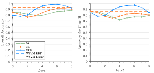
Figure 4. Semi-synthetic test classification results for unbalanced data sets. Accuracy and precision with respect to the number of nested multilevel $S_{0}\oplus S_{1}\oplus\dots\oplus S_{Level}$. The semi-synthetic data ${\mathcal{A}}_{\mathbf{A}}$ for class $\mathbf{A}$ is generated for $N_{\mathbf{A}}$ = 150, 250, 450, 1500 and 10000 realizations of class $\mathbf{A}$ using model (4). Similarly, class $\mathbf{B}$ dataset ${\mathcal{B}}_{N_{\mathbf{B}}}$ is generated $N_{\mathbf{B}}=100$ realizations with model (4). Since the size of ${\mathcal{B}}_{N_{\mathbf{B}}}$ is $N_{\mathbf{B}}=100$, then the number of realizations in ${\mathcal{A}}^{C}_{N_{\mathbf{A}}}$ is 150, 400, 1450, 9950 for $N_{\mathbf{A}}$ = 150, 450, 1500, and 10000 respectively. Conversely, the size of the data in ${\mathcal{A}}^{T}_{N_{\mathbf{A}}}$ is the same as for ${\mathcal{B}}_{N_{\mathbf{B}}}$, which is 50. The MOS filter is constructed from the data in ${\mathcal{A}}^{C}_{N_{\mathbf{A}}}$ with $M=39$ and applied to ${\mathcal{A}}^{T}_{N_{\mathbf{A}}}$ and ${\mathcal{B}}_{N_{\mathbf{B}}}$. These filtered datasets are then used to train a RBF SVM Gaussian kernel method. The performance of the machine is tested on semi-synthetic validation datasets ${\mathcal{A}}^{V}_{\tilde{N}_{\mathbf{A}}}$ and ${\mathcal{B}}^{V}_{\tilde{N}_{\mathbf{B}}}$, where $\tilde{N}_{\mathbf{A}}=\tilde{N}_{\mathbf{B}}=10,000$. We observe that the maximum accuracy and prediction is achieved for $N_{A}=10,000$. In contrast, the best results for the WSVM kernel and linear method with the unfiltered ${\mathcal{A}}^{T}_{N_{\mathbf{A}}}$ and ${\mathcal{B}}_{N_{\mathbf{B}}}$ datasets are shown as a dashed line.

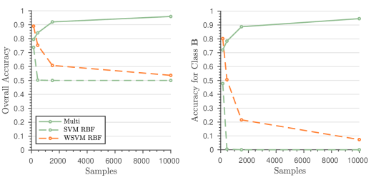
Figure 5. Accuracy and prediction comparison results between MSVM RBF, SVM RBF, and WSVM RBF as the number of samples in the training datasets increases for class $\mathbf{A}$ $({\mathcal{A}}_{{N_{\mathbf{A}}}})$. The accuracy and precision for the MSVM RBF classifier (multilevel filtered datasets) are plotted for $Level=6$ and with respect to the sample size of the datasets ${\mathcal{A}}_{N_{\mathbf{A}}}$. Notice that as as the dataset ${\mathcal{A}}_{N_{\mathbf{A}}}$ becomes more unbalanced, the accuracy and precision increase significantly. This is in contrast to SVM RBF and WSVM RBF, where the accuracy and precision degrade.

Test #2: The complexity of the classification problem is increased, where for each realization $u^{\mathbf{A}}_{M}(\mathbf{x},\omega_{k})$ by deforming the original datasets ${\mathcal{A}}_{N_{\mathbf{A}}}$ and ${\mathcal{A}}^{V}_{\tilde{N}_{\mathbf{A}}}$ (before updating them in Test #1). These realizations are updated as $u^{\mathbf{A}}_{M}(\mathbf{x},\omega_{k})\leftarrow sin(18u^{\mathbf{A}}_{M}(\mathbf{x},\omega_{k}))$. The realizations $u^{\mathbf{B}}_{M}(\mathbf{x},\omega_{k})$ in the original datasets ${\mathcal{B}}_{N_{\mathbf{B}}}$ and ${\mathcal{B}}^{V}_{\tilde{N}_{\mathbf{B}}}$ are also updated as $u^{\mathbf{B}}_{M}(\mathbf{x},\omega_{k})\leftarrow sin(18u^{\mathbf{B}}_{M}(\mathbf{x},\omega_{k}))$.

In Figure 6 (a) the accuracy results with respect to the number of realizations of ${\mathcal{A}}_{N_{\mathbf{A}}}$ are shown. We observe that the MSVM RBF method outperforms WSVM. (b) It is further shown that the MSVM RBF method is still robust towards unbalancing of the data. In fact, it benefits from the unbalanced datasets.

Test #3: The semi-synthetic data from Test #1 are again updated to make the classification problem much harder. For each realization $u^{\mathbf{A}}_{M}(\mathbf{x},\omega_{k})$ in the original datasets ${\mathcal{A}}_{N_{\mathbf{A}}}$ and ${\mathcal{A}}^{V}_{N_{\mathbf{A}}}$, is updated as $u^{\mathbf{A}}_{M}(\mathbf{x},\omega_{k})\leftarrow sin(20u^{\mathbf{A}}_{M}(\mathbf{x},\omega_{k}))$. The realizations $u^{\mathbf{B}}_{M}(\mathbf{x},\omega_{k})$ in the original datasets ${\mathcal{B}}_{N_{\mathbf{A}}}$ and ${\mathcal{B}}^{V}_{N_{\mathbf{A}}}$ are also updated as $u^{\mathbf{B}}_{M}(\mathbf{x},\omega_{k})\leftarrow sin(20u^{\mathbf{B}}_{M}(\mathbf{x},\omega_{k}))$. In Figure 7(a) the accuracy is shown for the updated data. Notice that the MSVM method significantly outperforms the SVM methods without the multilevel features, in particular, for the accuracy of Class $\mathbf{B}$. In Figure 7(b) we again observe that the accuracy significantly improves with the size of the realizations of ${\mathcal{A}}^{C}_{N_{\mathbf{A}}}$.

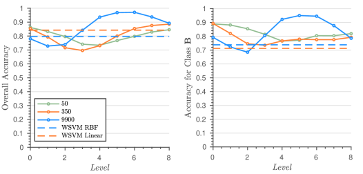
(a)

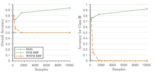
(b)

Figure 6. Semi-synthetic test classification results for modified unbalanced data sets. Test #1 is repeated but the realizations of the original datasets ${\mathcal{A}}_{N_{\mathbf{A}}}$, ${\mathcal{A}}^{V}_{N_{\mathbf{A}}}$, ${\mathcal{B}}_{N_{\mathbf{B}}}$ and ${\mathcal{B}}^{V}_{\tilde{N}_{\mathbf{B}}}$ are updated as $u^{\mathbf{A}}_{M}(\mathbf{x},\omega_{k})\leftarrow sin(18u^{\mathbf{A}}_{M}(\mathbf{x},\omega_{k}))$ and $u^{\mathbf{B}}_{M}(\mathbf{x},\omega_{k})\leftarrow sin(18u^{\mathbf{B}}_{M}(\mathbf{x},\omega_{k}))$. (a) The accuracy of all of the methods drops somewhat. However, it is clear that the MSVM RBF method outperforms and is more robust towards the increased complexity. (b) The MSVM RBF method improves with the unbalancing of the datasets. This is in contrast to SVM RBF and WSVM methods without the multilevel features.

Remark 7.

One key conclusion from these tests in that as the number of realizations are increased then the accuracy and precision of the RBF multilevel SVM filter in general increase. This is expected as the estimate of the covariance function in general becomes better and the separation of the classes improves. This is a good approach to deal with the difficult problem of unbalanced datasets. Thus the more unbalanced the data, the better the performance of the machine. This is in contrast to other methods that balance the dataset by subsampling, leading to information loss. Other methods balance the dataset by using a bootstrap method, but this approach can be unreliable.

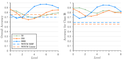
(a)

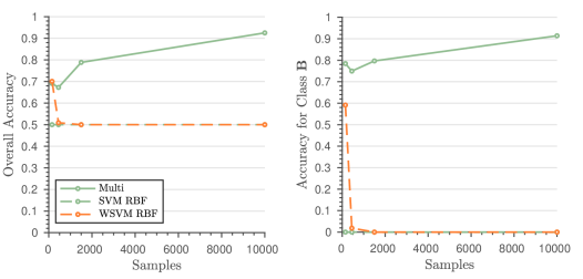
(b)

Figure 7. Semi-synthetic test classification results for modified unbalanced data sets. Test #1 is repeated but the realizations of the original datasets ${\mathcal{A}}_{N_{\mathbf{A}}}$, ${\mathcal{A}}^{V}_{N_{\mathbf{A}}}$, ${\mathcal{B}}_{N_{\mathbf{B}}}$ and ${\mathcal{B}}^{V}_{\tilde{N}_{\mathbf{B}}}$ are updated as $u^{\mathbf{A}}_{M}(\mathbf{x},\omega_{k})\leftarrow sin(20u^{\mathbf{A}}_{M}(\mathbf{x},\omega_{k}))$ and $u^{\mathbf{B}}_{M}(\mathbf{x},\omega_{k})\leftarrow sin(20u^{\mathbf{B}}_{M}(\mathbf{x},\omega_{k}))$. (a) For this dataset we observe that the MSVM RBF method significantly outperforms the best results from WSVM RBF and linear methods. In particular, for class $\mathbf{B}$ the accuracy degrades significantly. (b) As previously observed the MSVM RBF method improves with the unbalancing of the datasets. This is in contrast to SVM RBF and WSVM, which degrade significantly with the size of ${\mathcal{A}}_{N_{\mathbf{A}}}$.

4.2. Performance tests with Alzheimer’s Disease ADNI dataset

We now test the multilevel features with data from the Alzheimer’s Disease Neuroimaging Initiative (ADNI), a longitudinal multicenter study that was launched in 2003 designed to develop biomarkers for detection and tracking of Alzheimer’s disease [19]. This research is primarily focused on the plasma data of the ADNI participants. There are three groups of participants contained in this dataset. We have 209 measures of AD (Alzheimer’s Disease) participants, 742 samples from the MCI (Mild Cognitive Impairment) participants, and 112 samples from the CN (Cognitive Normal) participants. For each sample, there is a visit code of either BL (Baseline), or M12 (one year later) indicating the time the sample is collected. We performed tests on the M12 dataset, which contains 54 CN, 97 AD, and 346 MCI samples. After removing the features with more than 50% of missing values, the final number of features is 146.

We show the results for binary classification between M12 AD and CN samples. There are 54 CN and 97 AD samples respectively. The covariance matrix for the AD class using the extra 43 AD samples and the truncation parameter $M$ is set to 5. Both linear and RBF SVM are trained on the balanced dataset using leave-one-out cross validation. The study revealed that the RBF SVM on normalized projection coefficients achieved the highest accuracy of 89.11% for binary classification of M12 AD versus CN samples. On the other hand, RBF SVM on raw data only achieved an accuracy of 48.3%, with AUC scores of 0.9089 and 0.5657 for ROC curves respectively, indicating that the RBF SVM on projection coefficients had better predictive power (See Figure 8). For linear SVM, the highest accuracy on normalized projection coefficients and raw data are 54.51% and 63.92% and AUC scores are 0.5412 and 0.7456 respectively. Our results confirm that in the 146 features there are a combination of them that explain the AD outcome with high accuracy. For purposes of comparison the weighted SVM is also directly performed for the M12 AD vs CN binary classification. There is a small improvement to 64% accuracy for the Weighted RBF SVM.

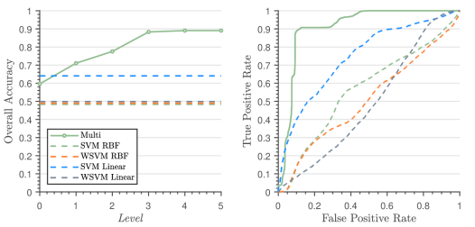
Figure 8. Comparison test for CN (Cognitive Normal subjects) vs AD participants. Accuracy and ROC curves (for the last level) for Multilevel features (with Radial SVM) compared to SVM with the original features are shown. The accuracy for the Multilevel features are plotted for each nested level. It is observed that the accuracy increases from 48.3% to 89.11% by using RBF SVM with the multilevel features. For the sake of comparison the weighted SVM is applied on the original features with linear kernel. For this case the accuracy increases to 64%. However, it is still significantly lower than the 89% accuracy obtained with the multilevel features.

5. Conclusions

In this paper we introduce a novel approach for creating features for machine learning based on stochastic functional analysis. From the covariance structure of a singular class of signals the problem is posed as a detection of an anomalous signal i.e. an unlikely realization of the baseline structure. A multilevel orthogonal basis is constructed to detect the magnitude and location of these anomalies. Signals from different classes that are hard to distinguish are mapped to small and to large coefficients with significantly greater separation. An SVM classifier can then more easily construct the separation boundary. The performance of the multilevel filter and the classifier depend on the availability of a rich dataset for construction of the truncated eigenspace. For signals that belong to a finite dimensional eigenspace and with sufficient data it can be shown that our approach leads to perfect classification (Theorem 3). The performance increases significantly as more data is available. This leads to a more accurate covariance and thus the separation between the classes improves. This is confirmed from the numerical results obtained from applying the multilevel filter on the semi-synthetic data created from the GCM dataset. Furthermore, tests on the ADNI Alzheimer’s Disease dataset gives rise to dramatic increases in accuracy (from 48% to 89% accuracy). There are still many avenues to explore based on the work in this paper. In particular:

1. This approach is being applied by A. McCormack and C. DeLisi to binary classification of kinetic properties of the rubisco enzyme [17]. This is an important topic that has been explored in [7, 16] in the context of carbon dioxide catalysis.

2. Extension of the multilevel method to multi class problems.

3. The effects of estimating the covariance structure on the accuracy of the classification.

4. Optimal estimation of the parameters $M$ and the nested level of the multilevel basis.

5. Since the multilevel filter leads to projection coefficients with greater distinguishability, this approach should be effective for ameliorating the problem of overfitting.

6. The approach developed in this paper is meant as a method to augment machine learning algorithms by using the multilevel features. For example, it can be application to Deep Neural Networks.

7. We shall explore the connections between the stochastic transformations and high dimensional data described by tensors [9, 11, 10, 14, 15].

References

- [1] J. E. Castrillón-Candás and Kevin Amaratunga. Spatially adapted multiwavelets and sparse representation of integral equations on general geometries. SIAM Journal on Scientific Computing, 24(5):1530–1566, 2003.
- [2] Julio E. Castrillón-Candás and Kevin Amaratunga. Fast estimation of continuous Karhunen-Loeve eigenfunctions using wavelets. IEEE Transactions on Signal Processing, 50(1):78–86, 2002.
- [3] Julio E. Castrillón-Candás and Mark Kon. Anomaly detection: A functional analysis perspective. Journal of Multivariate Analysis, 189:104885, 2022.
- [4] Julio E Castrillon-Candas and Mark Kon. Stochastic functional analysis and multilevel vector field anomaly detection, 2022. arXiv:2207.06229.
- [5] Nello Cristianini and John Shawe-Taylor. An Introduction to Support Vector Machines and Other Kernel-based Learning Methods. Cambridge University Press, 2000.
- [6] S. D’Heedene, K. Amaratunga, and J. E. Castrillón-Candás. Generalized hierarchical bases: a wavelet‐ritz‐galerkin framework for lagrangian FEM. Engineering Computations, 22(1):15–37, 2005.
- [7] Avi I. Flamholz, Noam Prywes, Uri Moran, Dan Davidi, Yinon M. Bar-On, Luke M. Oltrogge, Rui Alves, David Savage, and Ron Milo. Revisiting trade-offs between rubisco kinetic parameters. Biochemistry, 58(31):3365–3376, 2019. PMID: 31259528.
- [8] Helmut Harbrecht, Michael Peters, and Markus Siebenmorgen. Analysis of the domain mapping method for elliptic diffusion problems on random domains. Numerische Mathematik, 134(4):823–856, 2016.
- [9] Lifang He, Xiangnan Kong, Philip S. Yu, Ann B. Ragin, Zhifeng Hao, and Xiaowei Yang. Dusk: A dual structure-preserving kernel for supervised tensor learning with applications to neuroimages, 2014.
- [10] Lifang He, Chun-Ta Lu, Hao Ding, Shen Wang, Linlin Shen, Philip S. Yu, and Ann B. Ragin. Multi-way multi-level kernel modeling for neuroimaging classification. In 2017 IEEE Conference on Computer Vision and Pattern Recognition (CVPR), pages 6846–6854, 2017.
- [11] Lifang He, Chun-Ta Lu, Guixiang Ma, Shen Wang, Linlin Shen, Philip S. Yu, and Ann B. Ragin. Kernelized support tensor machines. In Doina Precup and Yee Whye Teh, editors, Proceedings of the 34th International Conference on Machine Learning, volume 70 of Proceedings of Machine Learning Research, pages 1442–1451. PMLR, 06–11 Aug 2017.
- [12] L. Horváth and P. Kokoszka. Inference for Functional Data with Applications. Springer, 2012.
- [13] P. Kokoszka and M. Reimherr. Introduction to Functional Data Analysis. CRC Press, 1 edition, 2017.
- [14] Kirandeep Kour, Sergey Dolgov, Peter Benner, Martin Stoll, and Max Pfeffer. A weighted subspace exponential kernel for support tensor machines, 2023.
- [15] Kirandeep Kour, Sergey Dolgov, Martin Stoll, and Peter Benner. Efficient structure-preserving support tensor train machine. Journal of Machine Learning Research, 24(4):1–22, 2023.
- [16] Stanislav Mazurenko, Zbynek Prokop, and Jiri Damborsky. Machine learning in enzyme engineering. ACS Catalysis, 10(2):1210–1223, 2020.
- [17] Adam McCormack and Charles P. DeLisi. Stochastic multilevel orthogonal subspaces for RuBisCO Engineering. In preparation, 2022.
- [18] Pramuditha Perera, Poojan Oza, and Vishal M. Patel. One-class classification: A survey, 2021.
- [19] R. C. Petersen, P. S. Aisen, L. A. Beckett, M. C. Donohue, A. C. Gamst, D. J. Harvey, Jr C. R. Jack, W. J. Jagust, L. M. Shaw, A. W. Toga, J. Q. Trojanowski, and M. W. Weiner. Alzheimer’s disease neuroimaging initiative (adni). Neurology, 74(3):201–209, 2010.
- [20] Sridhar Ramaswamy, Pablo Tamayo, Ryan Rifkin, Sayan Mukherjee, Chen-Hsiang Yeang, Michael Angelo, Christine Ladd, Michael Reich, Eva Latulippe, Jill P. Mesirov, Tomaso Poggio, William Gerald, Massimo Loda, Eric S. Lander, and Todd R. Golub. Multiclass cancer diagnosis using tumor gene expression signatures. Proceedings of the National Academy of Sciences, 98(26):15149–15154, 2001.
- [21] Christoph Schwab and Radu A. Todor. Karhunen–Loève approximation of random fields by generalized fast multipole methods. Journal of Computational Physics, 217(1):100 – 122, 2006. Uncertainty Quantification in Simulation Science.
- [22] Aik C. Tan, Daniel Q. Naiman, Lei Xu, Raimond L. Winslow, and Donald Geman. Simple decision rules for classifying human cancers from gene expression profiles. Bioinformatics, 21(20):3896–3904, 08 2005.
- [23] Petros Xanthopoulos and Talayeh Razzaghi. A weighted support vector machine method for control chart pattern recognition. Computers & Industrial Engineering, 70:134–149, 2014.