Optimization of the resonator-induced phase gate for superconducting qubits

Abstract

The resonator-induced phase gate is a two-qubit operation in which driving a bus resonator induces a state-dependent phase shift on the qubits equivalent to an effective $ZZ$ interaction. In principle, the dispersive nature of the gate offers flexibility for qubit parameters. However, the drive can cause resonator and qubit leakage, the physics of which cannot be fully captured using either the existing Jaynes-Cummings or Kerr models. In this paper, we adopt an ab-initio model based on Josephson nonlinearity for transmon qubits. The ab-initio analysis agrees well with the Kerr model in terms of capturing the effective $ZZ$ interaction in the weak-drive dispersive regime. In addition, however, it reveals numerous leakage transitions involving high-excitation qubit states. We analyze the physics behind such novel leakage channels, demonstrate the connection with specific qubits-resonator frequency collisions, and lay out a plan towards device parameter optimization. We show this type of leakage can be substantially suppressed using very weakly anharmonic transmons. In particular, weaker qubit anharmonicity mitigates both collision density and leakage amplitude, while larger qubit frequency moves the collisions to occur only at large anharmonicity not relevant to experiment. Our work is broadly applicable to the physics of weakly anharmonic transmon qubits coupled to linear resonators. In particular, our analysis confirms and generalizes the measurement-induced state transitions noted in Sank et al. Sank_Measurement-Induced_2016 and lays the groundwork for both strong-drive resonator-induced phase gate implementation and strong-drive dispersive qubit measurement.

I Introduction

Superconducting circuits Bouchiat_Quantum_1998 ; Nakamura_Coherent_1999 ; Friedman_Quantum_2000 ; Makhlin_Quantum-State_2001 ; Van_Quantum_2000 ; Martinis_Rabi_2002 ; Blais_Cavity_2004 ; Wallraff_Strong_2004 ; Koch_Charge_2007 ; Majer_Coupling_2007 provide a promising platform for quantum computation Shor_Algorithms_1994 ; Divincenzo_Quantum_1995 ; Barenco_Elementary_1995 ; Steane_Quantum_1998 ; Shor_Quantum_1998 ; Nielsen_Quantum_2002 . To ensure fault-tolerant quantum computation Shor_Fault_1996 ; Gottesman_Theory_1998 ; Kitaev_Fault_2003 ; Raussendorf_Fault_2007 , the underlying single- and two-qubit gates must satisfy certain error thresholds Gambetta_Building_2017 . Proposals for two-qubit gates fall into two major categories depending on the requirement for dynamic flux tunability. All-microwave architectures Paraoanu_Microwave_2006 ; Rigetti_Fully_2010 ; Chow_Microwave_2013 ; Cross_Optimized_2015 employ microwave pulses to entangle qubits, especially useful for fixed-frequency qubits such as the transmon Koch_Charge_2007 .

The Resonator-Induced Phase (RIP) gate Cross_Optimized_2015 ; Paik_Experimental_2016 ; Puri_High-Fidelity_2016 exploits an effective dynamic $ZZ$ (controlled-phase) interaction activated by a microwave pulse applied to a mediating bus resonator coupled to the qubits. The effective $ZZ$ rate is proportional to the resonator photon number and qubit-resonator dispersive couplings and inversely proportional to the resonator-drive detuning Cross_Optimized_2015 ; Puri_High-Fidelity_2016 . A theoretical proposal for the RIP gate was introduced in Ref. Cross_Optimized_2015 as a promising multi-qubit controlled-phase gate.

The most notable advantage of the RIP gate is the forgiving qubit frequency requirements. The RIP gate was experimentally demonstrated to entangle two fixed-frequency transmon qubits from as close as 380 MHz apart to as far as 1.8 GHz Paik_Experimental_2016 with fidelity per Clifford Knill_RB_2008 ; Magesan_Scalable_2011 ranging $93\%$ to $97\%$ (estimated gate fidelity $96\%$ to $98\%$). One unexplained experimental observation was that the measured fidelity showed improvement at smaller resonator-drive detuning. This did not agree with the detuning dependence expected for measurement-induced dephasing which should cause more error at small detuning. Moreover, this was not consistent with the leakage predictions of the dispersive Kerr model for the RIP gate Cross_Optimized_2015 .

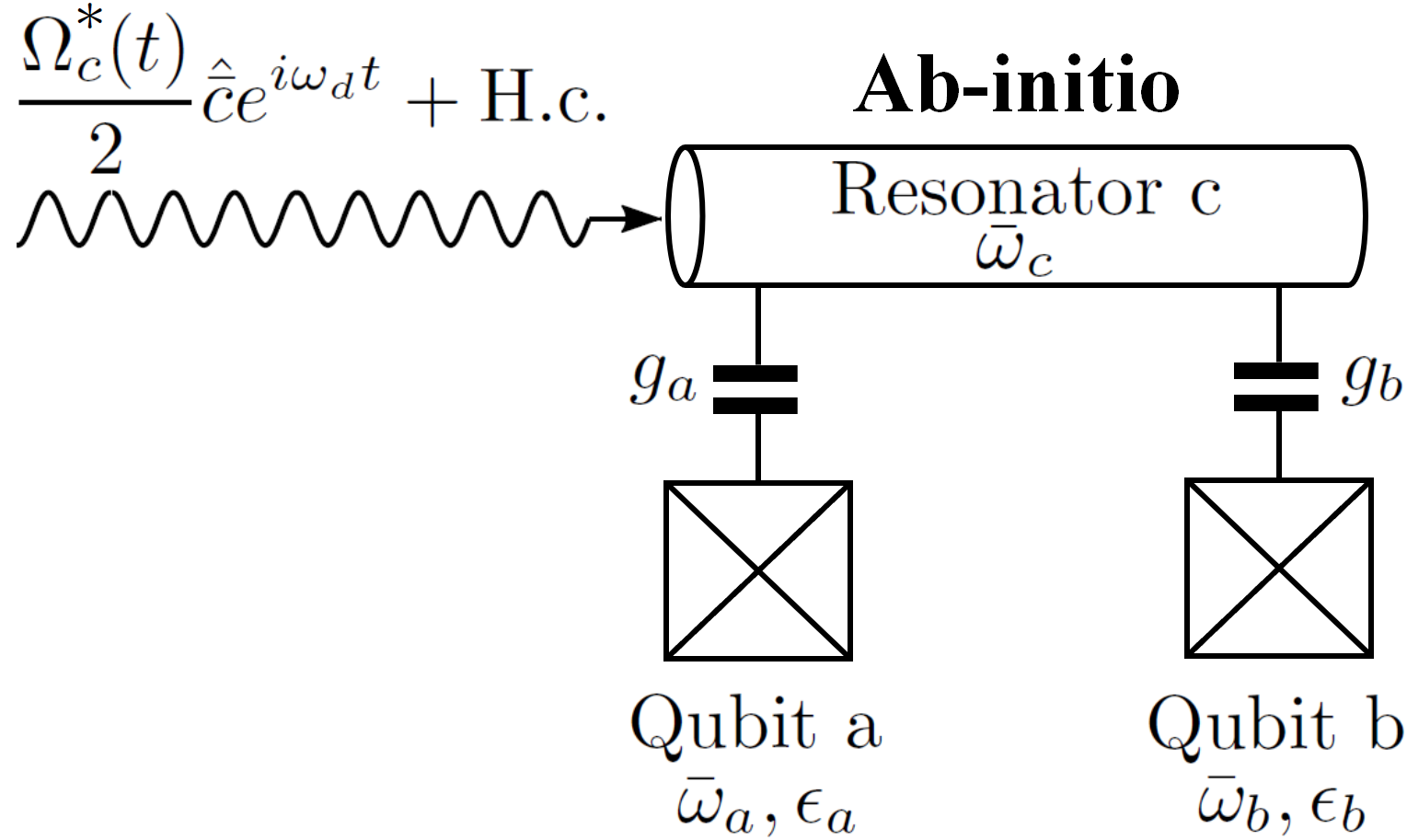
(a)

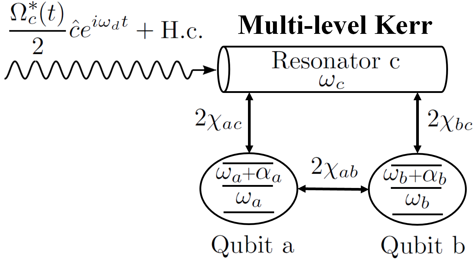
(b)

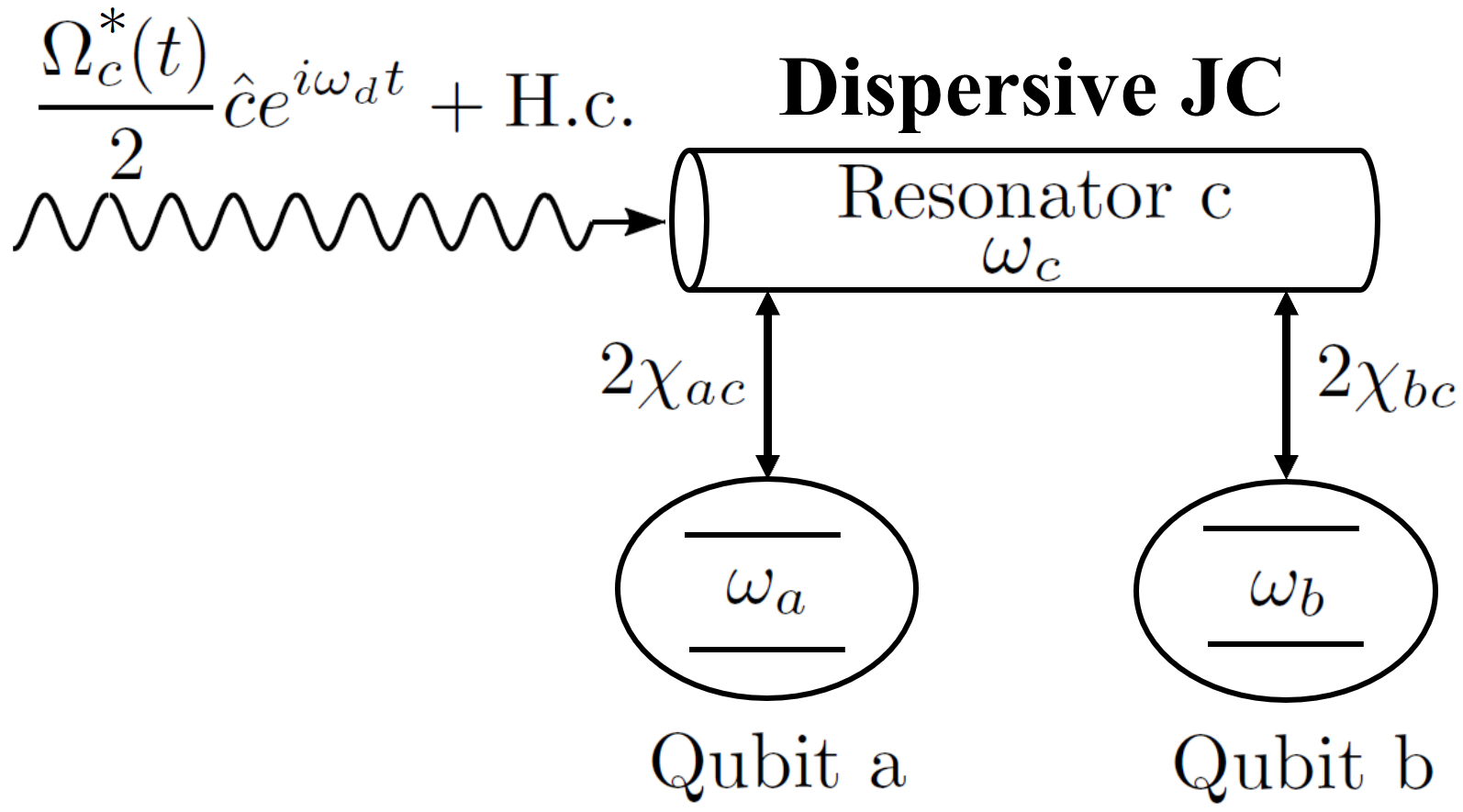
(c)

Figure 1: RIP gate under three levels of abstraction: (a) an ab-initio model based on the Josephson nonlinearity, (b) a multilevel Kerr model similar to Ref. Cross_Optimized_2015 (see Appendix B), and (c) a dispersive JC model similar to Ref. Puri_High-Fidelity_2016 (see Appendix A). When referring to the phenomenological models, we adopt the same level of precision as introduced by the original studies Cross_Optimized_2015 ; Puri_High-Fidelity_2016 as a point of comparison. For instance, only in the ab-initio model do we consider a RIP drive that acts on the bare (shown with a bar) resonator mode although such a modification and more could be made to improve the former models.

In this work, we characterize the RIP gate operation over a broad span of system parameters for two transmon qubits coupled to a linear resonator and propose experimentally relevant choices for optimal design. To this aim, we introduce an ab-initio model, based on the Josephson nonlinearity, that accounts for high-excitation states of the qubits. We show that the ab-initio analysis agrees with as well as extends the findings of previous studies based on multilevel Kerr Cross_Optimized_2015 ; Paik_Experimental_2016 and dispersive Jaynes-Cummings (JC) Puri_High-Fidelity_2016 models. Our study is focused on the coherent dynamics of the RIP gate, with an emphasis on the effective gate interactions, and on leakage as the main source of error. To derive an effective RIP Hamiltonian Maricq_Application_1982 ; Grozdanov_Quantum_1988 ; Rahav_Effective_2003 ; Mirrahimi_Modeling_2010 ; Goldman_Periodically_2014 ; Wang_Photon_2020 ; Magesan_Effective_2020 ; Malekakhlagh_First-Principles_2020 , we employ time-dependent Schrieffer-Wolff Perturbation Theory (SWPT) Schrieffer_Relation_1966 ; Bravyi_Schrieffer_2011 ; Bukov_Schrieffer_2016 ; Malekakhlagh_Lifetime_2020 ; Petrescu_Lifetime_2020 ; Magesan_Effective_2020 ; Malekakhlagh_First-Principles_2020 . We make comparisons between the effective gate parameters based on the JC, Kerr and ab-initio models and analyze the validity and breakdown of each model.

Our analysis of leakage reveals various distinct mechanisms that we categorize in terms of only the resonator (residual photons) Cross_Optimized_2015 ; Paik_Experimental_2016 , two qubits (qubit-qubit) similar to the cross-resonance (CR) gate Tripathi_Operation_2019 ; Malekakhlagh_First-Principles_2020 ; Hertzberg_Laser_2021 ; Zhang_High_2020 , one qubit and the resonator (qubit-resonator) similar to the standard readout scheme Sank_Measurement-Induced_2016 ; Lescanne_Escape_2019 ; Verney_Structural_2019 , and both qubits and the resonator (three-body). Revisiting the residual photons, we demonstrate order-of-magnitude improvement via DRAG Motzoi_Simple_2009 ; Gambetta_Analytic_2011 ; Malekakhlagh_Mitigating_2021 on the resonator. Qubit leakage, however, cannot be correctly captured by the phenomenological dispersive models Cross_Optimized_2015 ; Puri_High-Fidelity_2016 . This is due to the diagonal form of interactions with respect to the qubits subspace and the two-level assumption. Therefore, using the ab-initio model becomes essential.

We present extensive ab-initio simulation results for qubit leakage and identify the leakage clusters in terms of collisions between high-excitation qubit states and computational states with high photon number, generalizing Ref. Sank_Measurement-Induced_2016 . In particular, we show that qubit-resonator leakage involves very high excitation qubit states (5th-9th) compared to three-body leakage that involves also the medium-excitation states (2nd and above). These findings impose stringent trade-offs on parameter allocation for the RIP gate. As a general remedy for achieving both weaker leakage amplitude and less collision density, without compromising the effective RIP interaction, we propose to use (i) very weakly anharmonic transmons, with anharmonicity reduced down to approximately -200 MHz, and (ii) large qubit frequency of the order of 6 GHz.

The paper is organized as follows. In Sec. II, starting from the Josephson nonlinearity, we introduce an ab-initio model for the RIP gate and compare it with previous studies Cross_Optimized_2015 ; Puri_High-Fidelity_2016 . In Sec. III, we demonstrate our analytical method, based on time-dependent SWPT, for deriving an effective Hamiltonian for the RIP gate. We then make a comparison of the effective gate parameters ($IZ$, $ZI$ and $ZZ$) between the considered models. Section IV provides a characterization of leakage related to frequency collisions based on numerical simulation of the full dynamics. Lastly, in Sec. V, we summarize our findings towards system parameter optimization.

There are ten appendices that will be referred to throughout the paper. In Appendices A and B, using time-dependent SWPT, we provide the derivation of an effective gate Hamiltonian based on the dispersive JC Puri_High-Fidelity_2016 and the multilevel Kerr Cross_Optimized_2015 models, respectively. Appendix C discusses the normal mode representation of the ab-initio Hamiltonian using a canonical (Bogoliubov) transformation. Appendix D provides the details of a displacement transformation and the effective dynamics for the resonator mode. In Appendix E, we analyze the resonator response to basic RIP pulse shapes and provide a classical characterization of resonator leakage. Appendix F presents the derivation of an approximate ab-initio model via normal ordering of the nonlinear interactions. In Appendix G, we derive an effective RIP gate Hamiltonian based on the approximate ab-initio model of Appendix F. Appendix H discusses leakage mechanisms based on a three-level toy model. In Appendix I, we characterize the average gate error due to leakage. Lastly, Appendix J gives a brief summary of the numerical methods for leakage simulation.

II Model

For comparison, we consider several starting Hamiltonian models for the RIP gate and discuss how the underlying assumptions may limit precise analysis of certain aspects of the gate operation. To this aim, we analyze the RIP gate under the following levels of abstraction: (i) an exact ab-initio model for our numerical simulations, (ii) an approximate ab-initio model obtained by normal mode expansion of the former, (iii) a multilevel Kerr model similar to the one introduced in Ref. Cross_Optimized_2015 and (iv) a dispersive JC model similar to the one in Ref. Puri_High-Fidelity_2016 (see Fig. 1).

In the exact ab-initio model, we account for the Josephson nonlinearity of each qubit. The system and the drive Hamiltonian in the lab frame can be expressed in a unitless quadrature form as Koch_Charge_2007 ; Malekakhlagh_NonMarkovian_2016 ; Malekakhlagh_Origin_2016 ; Malekakhlagh_Cutoff-Free_2017 ; Didier_Analytical_2018 ; Malekakhlagh_Lifetime_2020 ; Petrescu_Lifetime_2020

$$\begin{split}\hat{\mathcal{H}}_{s}&=\sum\limits_{j=a,b}\frac{\bar{\omega}_{j}}{4}\left[(\hat{\bar{y}}_{j}-y_{gj})^{2}-\frac{2}{\epsilon_{j}}\cos(\sqrt{\epsilon_{j}}\hat{\bar{x}}_{j})\right]\\ &+\frac{\bar{\omega}_{c}}{4}\left(\hat{\bar{x}}_{c}^{2}+\hat{\bar{y}}_{c}^{2}\right)+\sum\limits_{j=a,b}g_{j}\hat{\bar{y}}_{j}\hat{\bar{y}}_{c}\;,\end{split}$$ (1a)

$$\hat{\mathcal{H}}_{d}(t) =-[\Omega_{cx}(t)\cos(\omega_{d}t)+\Omega_{cy}(t)\sin(\omega_{d}t)]\hat{\bar{y}}_{c}\;,$$ (1b)

where the qubit modes, the resonator mode and the drive are labeled as $a$, $b$, $c$ and $d$, respectively. The bar notation is used for quantities in the bare frame, to distinguish from the normal mode frame quantities that will be denoted with no bar. Moreover, $\bar{\omega}_{j}\equiv\sqrt{8E_{Cj}E_{Jj}}$ is the harmonic frequency, $\epsilon_{j}\equiv\sqrt{2E_{Cj}/E_{Jj}}=\varphi_{\text{j,ZPF}}^{2}$ is a small unitless anharmonicity measure and $y_{gj}\equiv n_{gj}/n_{\text{j,ZPF}}$ is the unitless gate charge for qubit $j=a,b$. Qubits are capacitively coupled to a common bus resonator with strength $g_{a}$ and $g_{b}$, respectively. The flux (phase) and charge (number) quadratures are written in a unitless form as $\hat{\bar{x}}_{k}\equiv\hat{\bar{k}}+\hat{\bar{k}}^{{\dagger}}$ and $\hat{\bar{y}}_{k}\equiv-i(\hat{\bar{k}}-\hat{\bar{k}}^{{\dagger}})$ for $k=a,b,c$. The drive acts capacitively on the resonator mode with time-dependent pulse amplitudes $\Omega_{cx}(t)$ and $\Omega_{cy}(t)$, and carrier frequency $\omega_{d}$. We take $\Omega_{cy}(t)$ as the main RIP pulse, while $\Omega_{cx}(t)$ provides additional degree of freedom used for DRAG Motzoi_Simple_2009 ; Gambetta_Analytic_2011 ; Malekakhlagh_Mitigating_2021 . Hamiltonian (1a)–(1b) serves as our point of reference and is used for the full numerical simulation.

For our analytical calculations, starting from Eqs. (1a)–(1b), we derive an approximate ab-initio model by first solving for the normal modes up to the harmonic theory, and then expanding the nonlinearity in the normal mode frame Malekakhlagh_Lifetime_2020 ; Petrescu_Lifetime_2020 similar to the black-box quantization Nigg_BlackBox_2012 and energy participation ratio Minev_EPR_2020 methods. Normal mode expansion converges faster when the transmon qubits are weakly anharmonic ($\epsilon\lessapprox 0.2$) and also when the effective interactions are implemented dispersively, i.e. large detuning between the qubits and the resonator as well as between the qubits themselves compared to qubits anharmonicity. This is an alternative to few-quantum-level models used commonly for systems operating in the straddling regime like the CR gate Magesan_Effective_2020 ; Tripathi_Operation_2019 ; Malekakhlagh_First-Principles_2020 . The normal mode representation of the RIP gate Hamiltonian reads

$$\begin{split}\hat{\mathcal{H}}_{s}&=\sum\limits_{k=a,b,c}\tilde{\omega}_{k}\hat{k}^{{\dagger}}\hat{k}+\sum\limits_{j=a,b}\sum\limits_{n=2}^{\infty}\frac{\bar{\omega}_{j}}{2}(-\epsilon_{j})^{n-1}\\ &\times\frac{\left[\left(\sum\limits_{k=a,b,c}u_{jk}\hat{k}\right)+\text{H.c.}\right]^{2n}}{(2n)!}\;,\end{split}$$ (2a)

$$\begin{split}\hat{\mathcal{H}}_{d}(t)&=[\Omega_{cx}(t)\cos(\omega_{d}t)+\Omega_{cy}(t)\sin(\omega_{d}t)]\\ &\times i[\sum\limits_{k=a,b,c}v_{ck}\hat{k}-\text{H.c.}]\;,\end{split}$$ (2b)

where $u_{jk}$ and $v_{jk}$, $j,k=a,b,c$, are the flux and charge hybridization coefficients that relate the corresponding bare and normal mode quadratures and are derived via a canonical (Bogoliubov) transformation Jellal_Two_2005 ; Merdaci_Entanglement_2020 ; Malekakhlagh_Lifetime_2020 (see Appendix C). Moreover, the normal mode harmonic frequencies are shown as $\tilde{\omega}_{k}$ in order to distinguish from the renormalized normal mode frequencies (no bar) that contain the static (Lamb) corrections.

Equations (2a)–(2b) demonstrate a rich variety of possible mixing both at the linear level through charge hybridization and the nonlinear level through flux hybridization. Equation (2b) shows that the RIP drive that is ideally supposed to populate the resonator mode will also act on the normal qubit modes through charge hybridization. For typical RIP parameters, the cross-drive on the qubits can be $10$% of the intended resonator drive. Furthermore, flux hybridization in Eq. (2a) leads to numerous nonlinear processes even up to the quartic expansion. To handle such complexity, we employ SNEG Zitko_Sneg_2011 in Mathematica, which allows sybmolic manipulation of bosonic operators, and derive an approximate ab-initio model for the RIP gate (see Appendix F).

To compare to previous studies, we also consider starting models similar to the ones introduced in Refs. Puri_High-Fidelity_2016 ; Cross_Optimized_2015 (see Fig. 1). Reference Cross_Optimized_2015 models the transmon qubits as weakly anharmonic Kerr oscillators as

$$\begin{split}\hat{\mathcal{H}}_{s,\text{Kerr}}&=\sum\limits_{j=a,b}\left[\omega_{j}\hat{n}_{j}+\frac{\alpha_{j}}{2}\hat{n}_{j}(\hat{n}_{j}-1)\right]\\ &+\omega_{c}\hat{n}_{c}+\sum\limits_{j,k=a,b,c\atop j>k}2\chi_{jc}\hat{n}_{j}\hat{n}_{c}\;,\end{split}$$ (3)

with the anharmonicity and dispersive couplings denoted by $\alpha_{j}$ and $2\chi_{jk}$ for $j,k=a,b,c$. The dispersive JC model Puri_High-Fidelity_2016 is similar to the Kerr model, but with two-level qubits as

$$\hat{\mathcal{H}}_{s,\text{JC}}=\sum\limits_{j=a,b}\frac{\omega_{j}}{2}\hat{\sigma}_{j}^{z}+\omega_{c}\hat{n}_{c}+\sum\limits_{j=a,b}\chi_{jc}\hat{n}_{c}\hat{\sigma}_{j}^{z}\;,$$ (4)

where $\hat{\sigma}_{j}^{z}\equiv\ket{1_{j}}\bra{1_{j}}-\ket{0_{j}}\bra{0_{j}}$. Moreover, in both studies, it is assumed that the drive acts only on the normal resonator mode as

$$\hat{\mathcal{H}}_{d}(t)=\frac{1}{2}\left[\Omega_{c}^{*}(t)\hat{c}e^{i\omega_{d}t}+\Omega_{c}(t)\hat{c}^{{\dagger}}e^{-i\omega_{d}t}\right]\;,$$ (5)

where $\Omega_{c}(t)\equiv\Omega_{cy}(t)-i\Omega_{cx}(t)$. Equations (3)–(5) have been modified with respect to the original studies to be consistent with our convention of denoting the full dispersive shift by $2\chi$ and the drive amplitude by $\Omega_{c}(t)$.

In terms of capturing the dynamic $ZZ$ (RIP) interaction, we find in the following that the dipsersive JC model is valid in the parameter regime $2\chi_{ac},2\chi_{bc}\ll|\Delta_{cd}|\ll|\Delta_{ad}|,|\Delta_{bd}|$, the multilevel Kerr model in $2\chi_{ac},2\chi_{bc}<|\Delta_{cd}|\ll|\Delta_{ad}|,|\Delta_{bd}|$ and the approximate ab-initio model in a broader resonator-drive detuning range of $2\chi_{ac},2\chi_{bc}<|\Delta_{cd}|<|\Delta_{ad}|,|\Delta_{bd}|$ (see Sec. III). In terms of capturing qubit leakage, however, the dispersive JC model cannot be used due to its two-level construction. The multilevel Kerr model is also unable to correctly predict qubit leakage for two reasons. Firstly, the starting Hamiltonian is diagonal with respect to the qubits preventing transitions out of the computational subspace. This can in principle be improved by adding phenomenological direct drive terms on the qubit modes. However, more importantly, Kerr estimates for transmon eigenenergies become less valid for high-excitation states, for which we observe considerable leakage due to frequency collisions. Therefore, using the exact ab-initio model is necessary in the characterization of qubit leakage discussed in Sec. IV.

III Effective RIP gate Hamiltonian

In Cross et al. Cross_Optimized_2015 , the gate operation was described within a Lindblad formalism by modeling the qubits as multilevel Kerr oscillators, and analytical estimates for the effective $ZZ$ rate were derived using the generalized P-representation Drummond_Generalised_1980 . Here, we analyze effective RIP interactions via SWPT and make a comparison between the aforementioned starting models. The effective RIP Hamiltonian takes the form

$$\hat{\mathcal{H}}_{\text{RIP,eff}}(t)\equiv\omega_{iz}(t)\frac{\hat{I}\hat{Z}}{2}+\omega_{zi}(t)\frac{\hat{Z}\hat{I}}{2}+\omega_{zz}(t)\frac{\hat{Z}\hat{Z}}{2}\;,$$ (6)

with a dynamic frequency shift for each qubit along with a two-qubit $ZZ$ interaction which consists of static and dynamic contributions. Our analytical method implements a series of unitary transformations from the lab frame to the effective diagonal frame of Eq. (6).

In Sec. III.1, we discuss a generic derivation of the effective Hamiltonian using time-dependent SWPT. In Sec. III.2, we apply it to the multilevel Kerr model, as a simpler case that captures the essential mechanism for the effective $ZZ$ interaction. Section III.3 compares the effective Hamiltonians found by applying the approach to all three models. Furthermore, detailed derivations of the effective RIP Hamiltonians based on the dispersive JC, the multilevel Kerr and the ab-initio models can be found in Appendices A, B and G, respectively.

III.1 Effective Hamiltonian via SWPT

To arrive at the effective Hamiltonian introduced in Eq. (6), we devise a unitary transformation $\hat{U}_{\text{diag}}(t)$ that maps the lab frame to the diagonal frame as

$$\hat{\mathcal{H}}_{I,\text{eff}}(t)\equiv\hat{U}_{\text{diag}}^{{\dagger}}(t)\left[\hat{\mathcal{H}}_{s}+\hat{\mathcal{H}}_{d}(t)-i\partial_{t}\right]\hat{U}_{\text{diag}}(t)\;.$$ (7)

It can be decomposed into intermediate unitary transformations as

$$\hat{U}_{\text{diag}}(t)\equiv\hat{D}[d_{c}(t)]\hat{U}_{0}(t)\hat{U}_{\text{SW}}(t)\;,$$ (8)

where $\hat{D}[d_{c}(t)]$, $\hat{U}_{0}(t)$ and $\hat{U}_{\text{SW}}(t)$ denote a coherent displacement transformation of the resonator mode, transformation to the interaction frame, and finally a SW transformation, respectively. In the following, we discuss each transformation in more detail.

A typical RIP drive can populate the resonator mode with several photons. The resonator response can therefore be effectively described in terms of classical (coherent) and quantum fluctuation parts. Formally, this is achieved by the displacement transformation

$$\hat{D}[d_{c}(t)]\equiv e^{d_{c}(t)\hat{c}^{{\dagger}}-d_{c}^{*}(t)\hat{c}}\;,$$ (9)

where $\hat{D}^{{\dagger}}[d_{c}(t)]\hat{c}\hat{D}[d_{c}(t)]=\hat{c}+d_{c}(t)$. We then set $d_{c}(t)$ to cancel out terms linear in $\hat{c}$ and $\hat{c}^{{\dagger}}$ in the displaced frame Hamiltonian. Up to the quartic expansion of the Josephson nonlinearity, this is equivalent to the response of a classical Kerr oscillator to the input RIP pulse. Under the rotating-wave approximation, one finds

$$\dot{\eta}_{c}(t)+i\Delta_{cd}\eta_{c}(t)+i\alpha_{c}|\eta_{c}(t)|^{2}\eta_{c}(t)=-\frac{i}{2}\Omega_{c}(t)\;,$$ (10)

where $\eta_{c}(t)\equiv d_{c}(t)e^{i\omega_{d}t}$ is the slowly-varying response amplitude, $\Delta_{cd}\equiv\omega_{c}-\omega_{d}$ is the resonator-drive detuning and $\alpha_{c}$ is the effective anharmonicity for the resonator [see Appendices A and D for the derivations based on the JC ($\alpha_{c}=0$) and the ab-initio models, respectively]. In Appendix E, based on Eq. (10), we have analyzed the resonator response and leakage in detail. Importantly, we show that using DRAG Motzoi_Simple_2009 ; Gambetta_Analytic_2011 ; Malekakhlagh_Mitigating_2021 can be helpful in suppressing the residual photons Cross_Optimized_2015 (see Sec. IV and Appendix E).

Next, in the displaced frame, we split the Hamiltonian into bare and interaction contributions as $\hat{\mathcal{H}}_{0}+\hat{\mathcal{H}}_{\text{int}}(t)$. The interaction frame Hamiltonian is then found by the unitary transformation $\hat{U}_{0}\equiv\exp(-i\hat{\mathcal{H}}_{0}t)$ as $\hat{\mathcal{H}}_{I}(t)\equiv\hat{U}_{0}^{{\dagger}}(t)\hat{\mathcal{H}}_{\text{int}}(t)\hat{U}_{0}(t)$. We note that there is flexibility in defining what bare and interaction contributions are. In particular, in Ref. Puri_High-Fidelity_2016 , cross-Kerr terms were not kept as bare contribution, which is justified for the explored parameter regime $|\Delta_{cd}|\gg|2\chi_{ac}|,|2\chi_{bc}|$. When referring to the dispersive JC model, we follow the same approximation as a point of comparison (see Appendix A). In Ref. Cross_Optimized_2015 and the ab-initio model, cross-Kerr interaction terms are kept in the bare Hamiltonian allowing for more precise modeling of the effective gate parameters for resonator-drive detunings comparable to the dispersive shift, i.e. $|\Delta_{cd}|\sim|2\chi_{ac}|,|2\chi_{bc}|$.

We then apply time-dependent SWPT to diagonalize the interaction frame Hamiltonian. The SW transformation is in principle a unitary transformation of the form,

$$\hat{U}_{\text{SW}}(t)=e^{-i\hat{G}(t)}\;,$$ (11)

where we expand the generator $\hat{G}(t)$ and the resulting effective Hamiltonian up to an arbitrary order in the interaction Gambetta_Analytic_2011 ; Magesan_Effective_2020 ; Malekakhlagh_Lifetime_2020 ; Petrescu_Lifetime_2020 ; Malekakhlagh_First-Principles_2020 ; Petrescu_Accurate_2021 ; Malekakhlagh_Mitigating_2021 . Here, we implement the perturbation up to the second order. The first order perturbation can be summarized as

$$\hat{\mathcal{H}}_{I,\text{eff}}^{(1)}(t)=\mathcal{S}\left(\hat{\mathcal{H}}_{I}(t)\right)\;,$$ (12a)

$$\dot{\hat{G}}_{1}(t)=\mathcal{N}\left(\hat{\mathcal{H}}_{I}(t)\right)\;,$$ (12b)

while the second order reads (see Appendix C of Ref. Malekakhlagh_First-Principles_2020 )

$$\hat{\mathcal{H}}_{I,\text{eff}}^{(2)}(t)=\mathcal{S}\Big{(}i[\hat{G}_{1}(t),\hat{\mathcal{H}}_{I}(t)]-\frac{i}{2}[\hat{G}_{1}(t),\dot{\hat{G}}_{1}(t)]\Big{)}\;,$$ (12c)

$$\dot{\hat{G}}_{2}(t)=\mathcal{N}\Big{(}i[\hat{G}_{1}(t),\hat{\mathcal{H}}_{I}(t)]-\frac{i}{2}[\hat{G}_{1}(t),\dot{\hat{G}}_{1}(t)]\Big{)}\;.$$ (12d)

In Eqs. (12a)–(12d), $\mathcal{S}(\bullet)$ and $\mathcal{N}(\bullet)$ denote the diagonal and off-diagonal parts of an operator. In summary, at each order in perturbation, we keep the diagonal contributions in the effective Hamiltonian and solve for a non-trivial SW generator that removes the off-diagonal part. For instance, first order off-diagonal terms in Eq. (12b) can produce diagonal contributions through 2nd order mixings that appear in terms of commutators in Eq. (12c).

Given the effective Hamiltonian in an extended Hilbert space, we read off the relevant gate parameters as

$$\omega_{iz}(t)\equiv\frac{1}{2}\text{Tr}\left\{\left(\hat{I}_{a}\otimes\hat{Z}_{b}\otimes\ket{0_{c}}\bra{0_{c}}\right)\cdot\hat{\mathcal{H}}_{I,\text{eff}}(t)\right\}\;,$$ (13a)

$$\omega_{zi}(t)\equiv\frac{1}{2}\text{Tr}\left\{\left(\hat{Z}_{a}\otimes\hat{I}_{b}\otimes\ket{0_{c}}\bra{0_{c}}\right)\cdot\hat{\mathcal{H}}_{I,\text{eff}}(t)\right\}\;,$$ (13b)

$$\omega_{zz}(t)\equiv\frac{1}{2}\text{Tr}\left\{\left(\hat{Z}_{a}\otimes\hat{Z}_{b}\otimes\ket{0_{c}}\bra{0_{c}}\right)\cdot\hat{\mathcal{H}}_{I,\text{eff}}(t)\right\},$$ (13c)

where $\hat{Z}\equiv\ket{0}\bra{0}-\ket{1}\bra{1}$. We have distinguished between the physical and the logical Pauli operators, used in Eqs. (4) and (13a)–(13c) such that $\hat{Z}=-\hat{\sigma}^{z}$. The effective Hamiltonian is defined in the displaced frame, and hence the zero-photon subspace in Eqs. (13a)–(13c) corresponds to no excitations beyond the coherent photon number $|\eta_{c}(t)|^{2}$. In experimental results, it is more common to report the full $ZZ$ rate, which is twice the value quoted in this paper.

In order to calibrate a controlled-phase gate of rotation angle $\theta_{zz}$ we need to set $\int_{0}^{\tau}dt^{\prime}\omega_{zz}(t^{\prime})=\theta_{zz}$, where $\omega_{zz}(t)=\omega_{zz}^{(0)}+\omega_{zz}^{(2)}(t)+O(\hat{\mathcal{H}}_{I}^{4})$. In particular, $\theta_{zz}=\pi/2$ is equivalent to CNOT up to single-qubit Hadamard and $Z$ rotations as

$$\quad\quad\hat{U}_{\text{CZ}}=\exp\left[-i\frac{\pi}{4}\left(\hat{I}\hat{I}-\hat{I}\hat{Z}-\hat{Z}\hat{I}+\hat{Z}\hat{Z}\right)\right]\;,$$ (14a)

$$\quad\quad\hat{U}_{\text{CX}}=\hat{I}\hat{H}\cdot\hat{U}_{\text{CZ}}\cdot\hat{I}\hat{H}\;,$$ (14b)

with $\hat{U}_{\text{CZ}}$, $\hat{U}_{\text{CX}}$ and $\hat{H}$ denoting the controlled-$Z$, controlled-$X$ and Hadamard operations.

The procedure outlined in this section can be extended to a Lindblad master equation to arrive at an effective $ZZ$ rate that accounts for the resonator decay rate $\kappa_{c}$ Cross_Optimized_2015 . The result can be obtained by replacing $\omega_{c}\rightarrow\omega_{c}-i\kappa_{c}/2$ and reading off the real part of Eq. (13c) (see Cross et al. Cross_Optimized_2015 for more detail).

III.2 Kerr model

We next analyze the effective Hamiltonian and gate parameters based on the multilevel Kerr model (see Appendix B for derivation). The perturbative description of the effective Hamiltonian is valid when $|\chi_{jc}\eta_{c}(t)|<|\Delta_{cd}|$ for $j=a,b$.

The lowest order correction to the effective Hamiltonian reads

$$\hat{\mathcal{H}}_{I,\text{eff}}^{(1)}(t)=2\chi_{ac}|\eta_{c}(t)|^{2}\hat{n}_{a}+2\chi_{bc}|\eta_{c}(t)|^{2}\hat{n}_{b}\;,$$ (15)

consisting of a dynamic frequency shift equal to $2\chi$ per resonator photon number for each qubit. Up to the second order, we find

$$\begin{split}\hat{\mathcal{H}}_{I,\text{eff}}^{(2)}(t)=&-8\chi_{ac}\chi_{bc}\hat{\mathcal{A}}_{\eta}(t)\hat{n}_{a}\hat{n}_{b}\\ &-4\chi_{ac}^{2}\hat{\mathcal{A}}_{\eta}(t)\hat{n}_{a}^{2}\\ &-4\chi_{bc}^{2}\hat{\mathcal{A}}_{\eta}(t)\hat{n}_{b}^{2}\;,\\ \end{split}$$ (16a)

which contains an effective number-number interaction as well as an anharmonic shift of the qubit eigenfrequencies. The drive dependence of the effective interaction can be compactly written in terms of the response function

$$\hat{\mathcal{A}}_{\eta}(t)\equiv\text{Im}\left\{\int^{t}dt^{\prime}\eta_{c}(t)\eta_{c}^{*}(t^{\prime})e^{i\hat{\Delta}_{cd}(t-t^{\prime})}\right\}\;,$$ (16b)

$$\hat{\Delta}_{cd}\equiv\Delta_{cd}+2\chi_{ac}\hat{n}_{a}+2\chi_{bc}\hat{n}_{b}\;,$$ (16c)

where the operator-valued detuning $\hat{\Delta}_{cd}$ encodes the qubit-state-dependent phase for the resonator (see Fig. 2). In the adiabatic limit, for which the spectral content of the drive has negligible overlap with the resonator-drive detuning $\Delta_{cd}$, we can approximate $\hat{\mathcal{A}}_{\eta}(t)$ as

$$\begin{split}\hat{\mathcal{A}}_{\eta}(t)=\frac{|\eta_{c}(t)|^{2}}{\hat{\Delta}_{cd}}+\frac{\text{Im}\left\{\eta_{c}(t)\dot{\eta}_{c}^{*}(t)\right\}}{\hat{\Delta}_{cd}^{2}}+O\left(\frac{\eta_{c}(t)\ddot{\eta}_{c}^{*}(t)}{\hat{\Delta}_{cd}^{3}}\right),\end{split}$$ (17)

where the first and the second terms are known as the dynamic and geometric Pechal_geometric_2012 ; Bohm_Geometric_2013 ; Cross_Optimized_2015 contributions. The geometric correction becomes pertinent for relatively fast pulses with spectral widths comparable to the resonator-drive detuning. Because such pulses lead to significant resonator leakage (see Appendix E), we consider only the leading dynamic contribution which is proportional to the photon number $|\eta_{c}(t)|^{2}$.

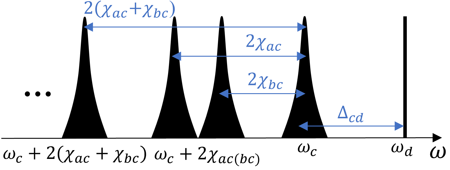
Figure 2: Schematic of the four (computational) qubit-state-dependent frequencies for the resonator based on the Kerr model.

Using Eqs. (13a)–(13c), we read off the gate parameters by projecting the effective Hamiltonian in Eqs. (15) and (16a) onto the computational subspace. The lowest order Hamiltonian contains dynamic frequency shifts for the qubits as

$$\omega_{iz}^{(1)}(t)=-2\chi_{bc}|\eta_{c}(t)|^{2}\;,$$ (18a)

$$\omega_{zi}^{(1)}(t)=-2\chi_{ac}|\eta_{c}(t)|^{2}\;.$$ (18b)

The second order dynamic frequency shifts read

$$\begin{split}\omega_{iz}^{(2)}(t)=\frac{1}{2}\left[\frac{2\chi_{bc}(\Delta_{cd}+4\chi_{bc})}{\Delta_{cd}+2\chi_{bc}}-\frac{\Delta_{cd}^{2}}{\Delta_{cd}+2\chi_{ac}}\right.\\ \left.+\frac{\Delta_{cd}^{2}}{\Delta_{cd}+2(\chi_{bc}+\chi_{ac})}\right]|\eta_{c}(t)|^{2}\;,\end{split}$$ (19a)

$$\begin{split}\omega_{zi}^{(2)}(t)=\frac{1}{2}\left[\frac{2\chi_{ac}(\Delta_{cd}+4\chi_{ac})}{\Delta_{cd}+2\chi_{ac}}-\frac{\Delta_{cd}^{2}}{\Delta_{cd}+2\chi_{bc}}\right.\\ \left.+\frac{\Delta_{cd}^{2}}{\Delta_{cd}+2(\chi_{ac}+\chi_{bc})}\right]|\eta_{c}(t)|^{2}\;.\end{split}$$ (19b)

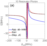
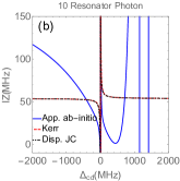
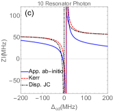
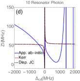
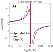
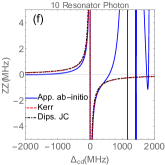
Figure 3: Comparison between the phenomenological and the approximate ab-initio models under adiabatic approximation as a function of $\Delta_{cd}$ and maximum photon number $|\eta_{c}(t)|^{2}\rightarrow|\eta_{c,\text{ss}}|^{2}\approx(\Omega_{c}/2\Delta_{cd})^{2}=10$. For the ab-initio model, system parameters are $E_{Ja}/2\pi=14250$, $E_{Ca}/2\pi=255$ ($\bar{\omega}_{a}/2\pi\approx 5391.660$), $E_{Jb}/2\pi=17000$, $E_{Cb}/2\pi=275$ ($\bar{\omega}_{b}/2\pi\approx 6115.550$), $\bar{\omega}_{c}/2\pi=7000$, with couplings $g_{a}/2\pi=150$ and $g_{b}/2\pi=85$, which up to the sextic expansion yields $2\chi_{ac}/2\pi\approx-4.863$ and $2\chi_{bc}/2\pi\approx-4.910$ (all in MHz). Gate charge is set to zero for simplicity. Phenomenological models adopt the same dispersive shifts and normal mode frequencies. The left column shows small–medium resonator-drive detuning where the RIP gate is typically implemented. The right column shows the same traces plotted over a wider detuning range to demonstrate that the ab-initio theory captures the renormalization of the gate parameters due to additional interaction forms involving qubit resonances (see Appendix G).

Furthermore, there is a dynamic $ZZ$ term corresponding to the intended RIP interaction,

$$\omega_{zz}^{(2)}(t)=\frac{-4\chi_{ac}\chi_{bc}(\Delta_{cd}+\chi_{ac}+\chi_{bc})\Delta_{cd}|\eta_{c}(t)|^{2}}{(\Delta_{cd}+2\chi_{ac})(\Delta_{cd}+2\chi_{bc})[\Delta_{cd}+2(\chi_{ac}+\chi_{bc})]},$$ (19c)

which is proportional to the resonator photon number and the dispersive shift for each qubit. There are four distinct poles at $\Delta_{cd}\approx 0$ [hidden in $\eta_{c}(t)$ in the adiabatic limit], $\Delta_{cd}=-2\chi_{ac}$, $\Delta_{cd}=-2\chi_{bc}$ and $\Delta_{cd}=-2(\chi_{ac}+2\chi_{bc})$ corresponding to resonance between the drive frequency and the resonator frequency for the computational states $\ket{0_{a}0_{b}}$, $\ket{1_{a}0_{b}}$, $\ket{0_{a}1_{b}}$ and $\ket{1_{a}1_{b}}$, respectively (see Fig. 2). In the limit where $\chi_{ac}=\chi_{bc}=\chi$, we recover the expression quoted in Refs. Cross_Optimized_2015 ; Paik_Experimental_2016 as $-4\chi^{2}\Delta_{cd}|\eta_{c}(t)|^{2}/[(\Delta_{cd}+2\chi)(\Delta_{cd}+4\chi)]$. Moreover, if the detuning is much larger than the dispersive shifts, we reach a simpler expression as $-4\chi^{2}|\eta_{c}(t)|^{2}/\Delta_{cd}$ in agreement with the dispersive JC model Puri_High-Fidelity_2016 .

Note that the RIP interaction sits on top of a static $ZZ$ rate that is captured only by the multilevel models (Kerr and ab-initio). In terms of an effective qubit-qubit exchange interaction

$$J\approx\left[\frac{(\bar{\Sigma}_{ab}-2\bar{\omega}_{c})}{2\bar{\Delta}_{ac}\bar{\Delta}_{bc}}-\frac{(\bar{\Sigma}_{ab}+2\bar{\omega}_{c})}{2\bar{\Sigma}_{ac}\bar{\Sigma}_{bc}}\right]g_{a}g_{b}\;,$$ (20a)

with $$\bar{\Sigma}_{jk}\equiv\bar{\omega}_{j}+\bar{\omega}_{k} \bar{\Delta}_{jk}\equiv\bar{\omega}_{j}-\bar{\omega}_{k}$$ and , the multilevel Kerr model Cross_Optimized_2015 ; Magesan_Effective_2020 predicts

$$\omega_{zz}^{(0)}\approx\frac{J^{2}}{\Delta_{ab}-\alpha_{b}}-\frac{J^{2}}{\Delta_{ab}+\alpha_{a}}\;.$$ (20b)

Static $ZZ$ interaction reduces the on/off contrast of the $ZZ$ gate and can be detrimental to most gate operations. However, there are various methods for its suppression: (i) large qubit-qubit detuning compared to qubit anharmonicity [see Eq. (20b)], (ii) fast tunable couplers Chen_Qubit_2014 , (iii) destructive interference between multiple couplers Mundada_Suppression_2019 ; Kandala_Demonstration_2020 , (iii) combining qubits with opposite anharmonicity Ku_Suppression_2020 , and (iv) dynamics Stark tones (siZZle) Wei_Quantum_2021 ; Mitchell_Hardware_2021 . In particular, method (iii) has shown significant improvement in reducing the static $ZZ$ down to 0.1 KHz for a test RIP device consisting of six qubits Kumph_Novel_APS2021 .

III.3 Comparison and discussion

We next study the RIP gate parameters in more detail and make a comparison between the various starting models introduced in Sec. II. Figure 3 presents the effective RIP gate parameters as a function of resonator-drive detuning for fixed photon number.

In particular, in terms of agreement for the dynamic $ZZ$ rate, we recognize three regions of operation depending on the relation between the resonator-drive detuning $\Delta_{cd}$, qubit-drive detunings $\Delta_{ad},\Delta_{bd}$ and the dispersive shifts $2\chi_{ac}$ and $2\chi_{bc}$:

• Small detuning ($|\Delta_{cd}|\sim~{}2|\chi_{ac}|,\ 2|\chi_{bc}|$) — The ab-initio and the Kerr Cross_Optimized_2015 models agree well and both predict a local maximum for the $ZZ$ rate for $\Delta_{cd}<0$ [Fig. 3(e)]. The local maximum is a result of having multiple relatively close poles at $\Delta_{cd}=-2\chi_{ac},-2\chi_{bc}$ and $\Delta_{cd}=-2\chi_{ac}-2\chi_{bc}$.

• Medium detuning ($2|\chi_{ac}|,\ 2|\chi_{bc}|\ll|\Delta_{cd}|\ll|\Delta_{ad}|,|\Delta_{bd}|$) — RIP drive frequency is closer to the resonator than to the qubit frequencies. Moreover, resonator-drive detuning is sufficiently larger than the dispersive shifts such that the qubit-state dependence of the poles is less noticeable. Consequently, all models agree.

• Large detuning ($2|\chi_{ac}|,\ 2|\chi_{bc}|\ll|\Delta_{cd}|\sim|\Delta_{ad}|,|\Delta_{bd}|$) — Resonator-drive and qubit-drive detunings are comparable. Therefore, there are additional processes, beyond dispersive JC and Kerr interactions, that renormalize the gate parameters (see Appendices F and G). This region is not necessarily relevant to RIP gate implementation but is a natural extension of our comparison which quantifies the validity of the phenomenological models [Fig. 3(f)].
  

In terms of the RIP interaction, the ab-initio model agrees well with the former phenomenological models in their intended resonator-drive detuning regimes. However, according to Fig. 3, we observe a large deviation between the dynamic frequency shifts predicted by the ab-initio theory compared to the phenomenological models in all regions of operation. We find the source of this deviation to be contributions of the form $\hat{\mathcal{H}}_{\text{qd}}(t)\equiv\sum_{j=a,b}[\lambda_{j}(t)\hat{j}e^{i\omega_{d}t}+\text{H.c.}]$ that act as direct drive terms on the qubits. Here, $\lambda_{j}(t)$ denotes the effective drive amplitude on qubit $j=a,b$ and contains contributions from linear charge hybridization and nonlinear mode mixing through flux hybridization (see Appendices F and G).

In summary, larger dispersive shifts, stronger RIP drive amplitude and smaller resonator-drive detuning all contribute to a stronger $ZZ$ interaction. However, we have to account also for the trade-off between a strong dynamic $ZZ$ rate and the corresponding unwanted increase in both resonator and qubit leakage. Our analysis of leakage reveals further restrictions on the choice for qubit frequency, anharmonicity and RIP drive parameters, which we discuss in Sec. IV and Appendix E.

IV Leakage

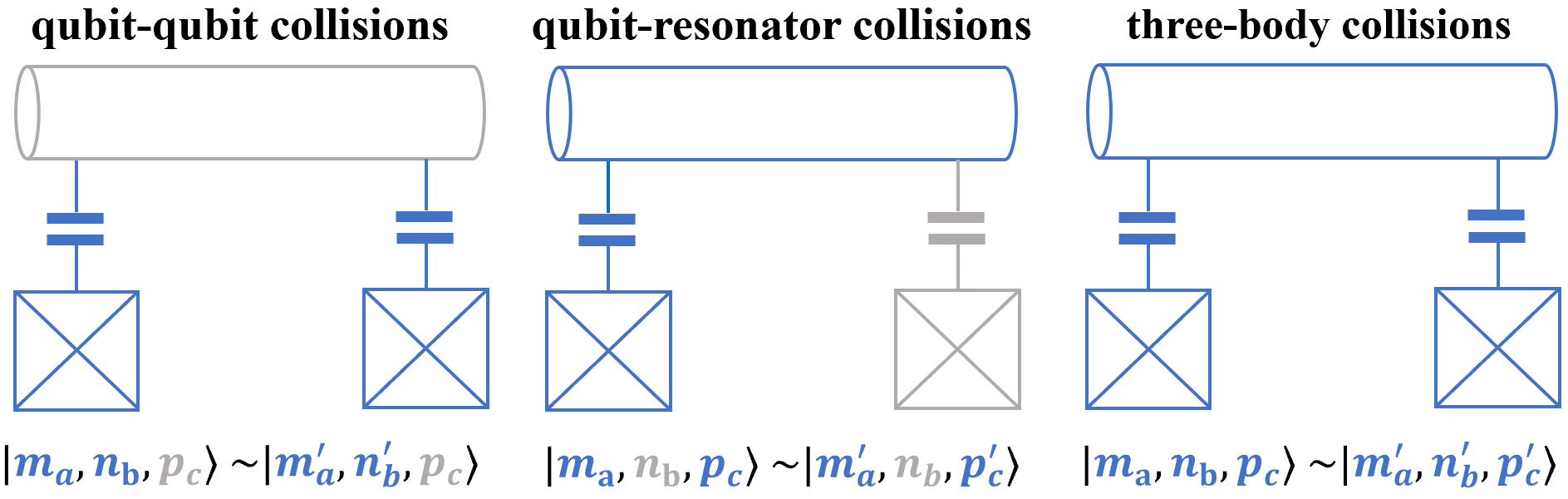
Figure 4: Universe of collisions involving two transmon qubits that are connected via a common bus resonator. The possibilities can be summarized as (i) qubit-qubit collisions Magesan_Effective_2020 ; Malekakhlagh_First-Principles_2020 ; Hertzberg_Effects_2020 , (ii) qubit-resonator collisions Sank_Measurement-Induced_2016 and (iii) three-body collisions. Symbol “$\sim$” denotes collision (degeneracy) between system states.

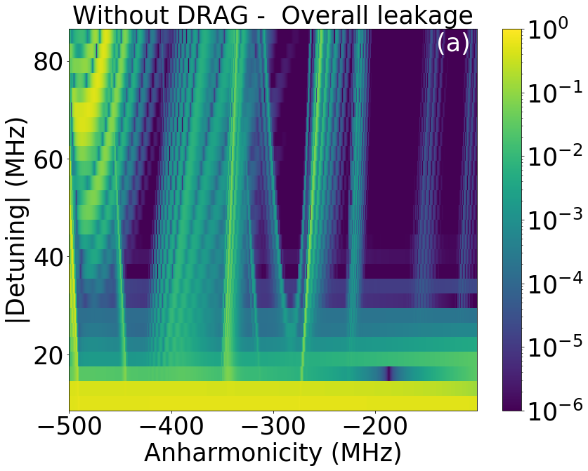
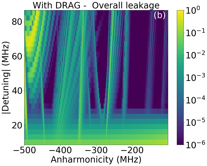
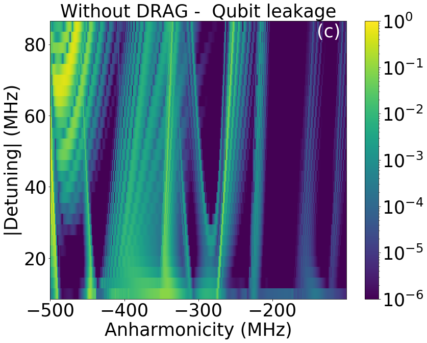
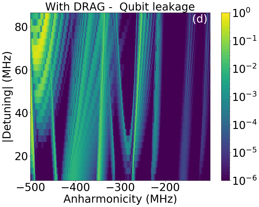
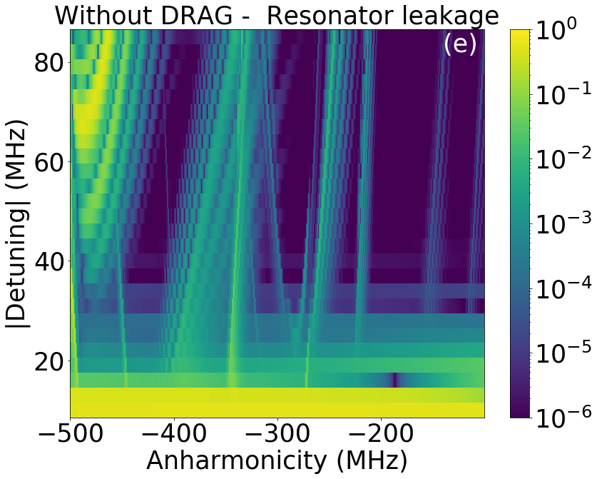
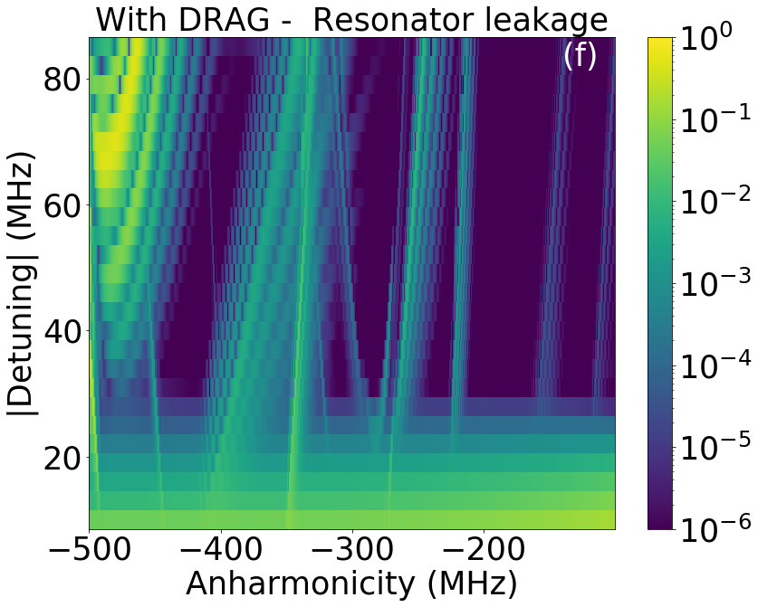
Figure 5: Qubit-resonator case — Overall, qubit and resonator leakages for $\omega_{a}/2\pi\approx 5140$ MHz, $\omega_{c}/2\pi\approx 6971$ MHz, $2\chi_{ac}/2\pi\approx-5.57$ MHz, fixed maximum photon number $[\Omega_{c}/(2\Delta_{cd})]^{2}\approx 16$ and fixed gate charge set to $0.37$ as a function of qubit anharmonicity and resonator-drive detuning. The initial state is set as $\ket{\Psi(0)}=(1/\sqrt{2})(\ket{0_{a}}+\ket{1_{a}})\otimes\ket{0_{c}}$ to allow leakage from both qubit states in a single run. The results here are for $\omega_{d}>\omega_{c}$. We confirmed numerically that $\omega_{d}<\omega_{c}$ leads to more resonator leakage consistent with additional $2\chi$-shifted poles in Eq. (16c) and Fig. 2. The resonator is driven with a nested cosine pulse [Eq. 21] of $\tau=200$ ns. The left (right) column present results without (with) DRAG on the resonator given by Eqs. (22a)–(22b).

RIP gate leakage can be separated into a background leakage, also called residual photons, due to the non-adiabaticity of the drive pulse and the resonator, and leakage to specific system states due to frequency collisions. The background leakage is comparably easy to understand and control, as its ratio to the intended photon number depends primarily on the overlap of the pulse’s spectrum with the resonator frequency via the collective quantity $\Delta_{cd}\tau$, with $\tau$ being the pulse (rise) time. Therefore, to keep the background leakage constant, while making the pulse twice as fast, the most basic solution is to double $\Delta_{cd}$ and $\Omega_{c}$. A more involved control scheme for mitigating the background leakage, however, is to filter the pulse spectrum at $\Delta_{cd}$. We show that adding a DRAG pulse to the resonator works as an effective filter (see also Appendix E).

Focusing on the leakage due to frequency collisions, depending on what circuit elements participate in the exchange of excitations, three categories arise (see Fig. 4): (i) Qubit-qubit collisions Magesan_Effective_2020 ; Malekakhlagh_First-Principles_2020 ; Hertzberg_Effects_2020 , (ii) qubit-resonator collisions Sank_Measurement-Induced_2016 , and (iii) three-body collisions. Qubit-qubit collisions occur in the zero (fixed)-photon subspace of the resonator when the qubits’ detuning is approximately an integer multiple of the qubits’ anharmonicity. Having qubit-qubit detuning away from the straddling regime minimizes the leakage due to such inter-qubit collisions. Qubit-resonator collisions occur between high- and low-excitation states of one of the qubits and the resonator while the other qubit is in a fixed state. More involved three-body collisions are also possible where both qubits and the resonator participate.

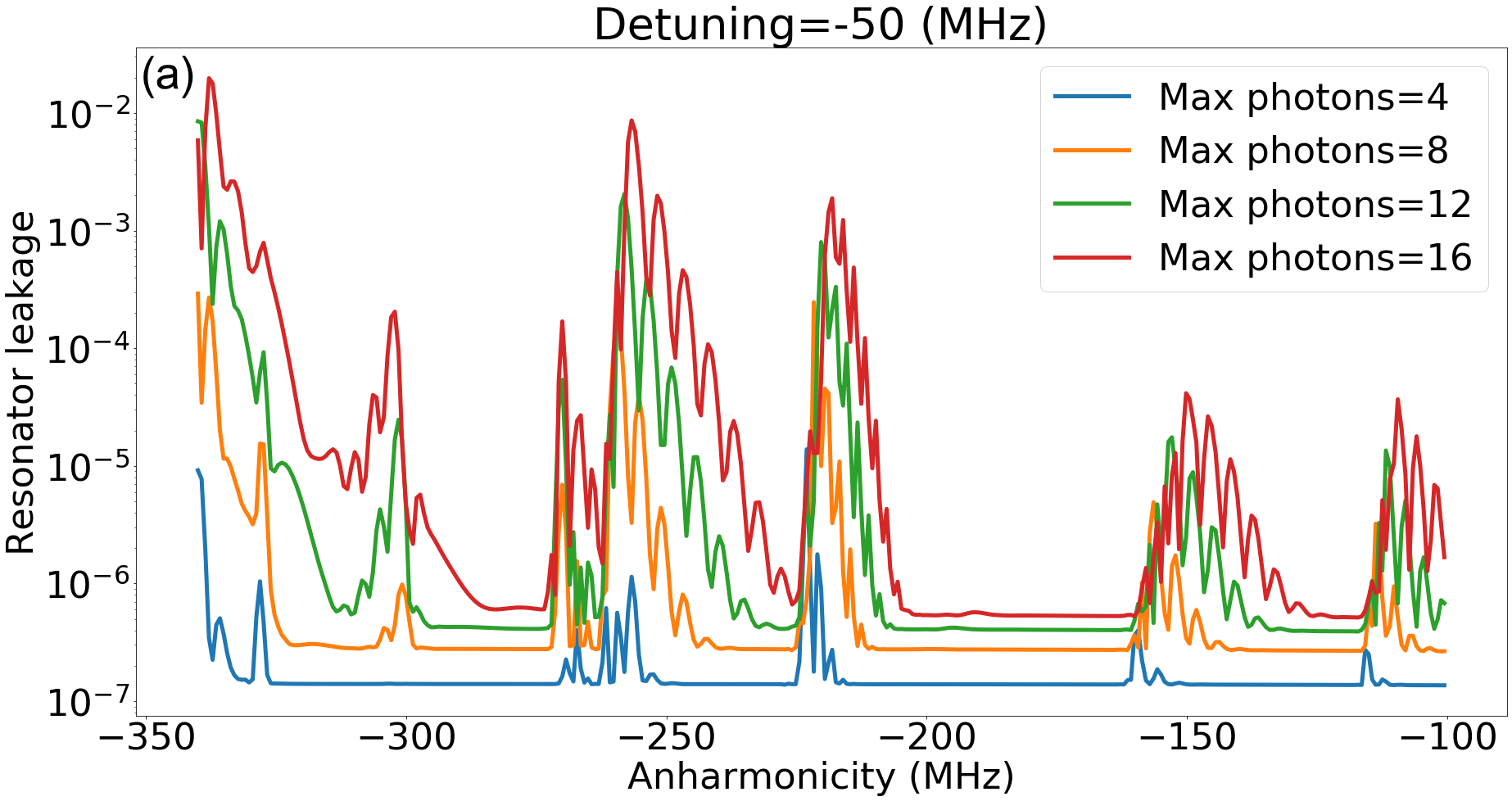
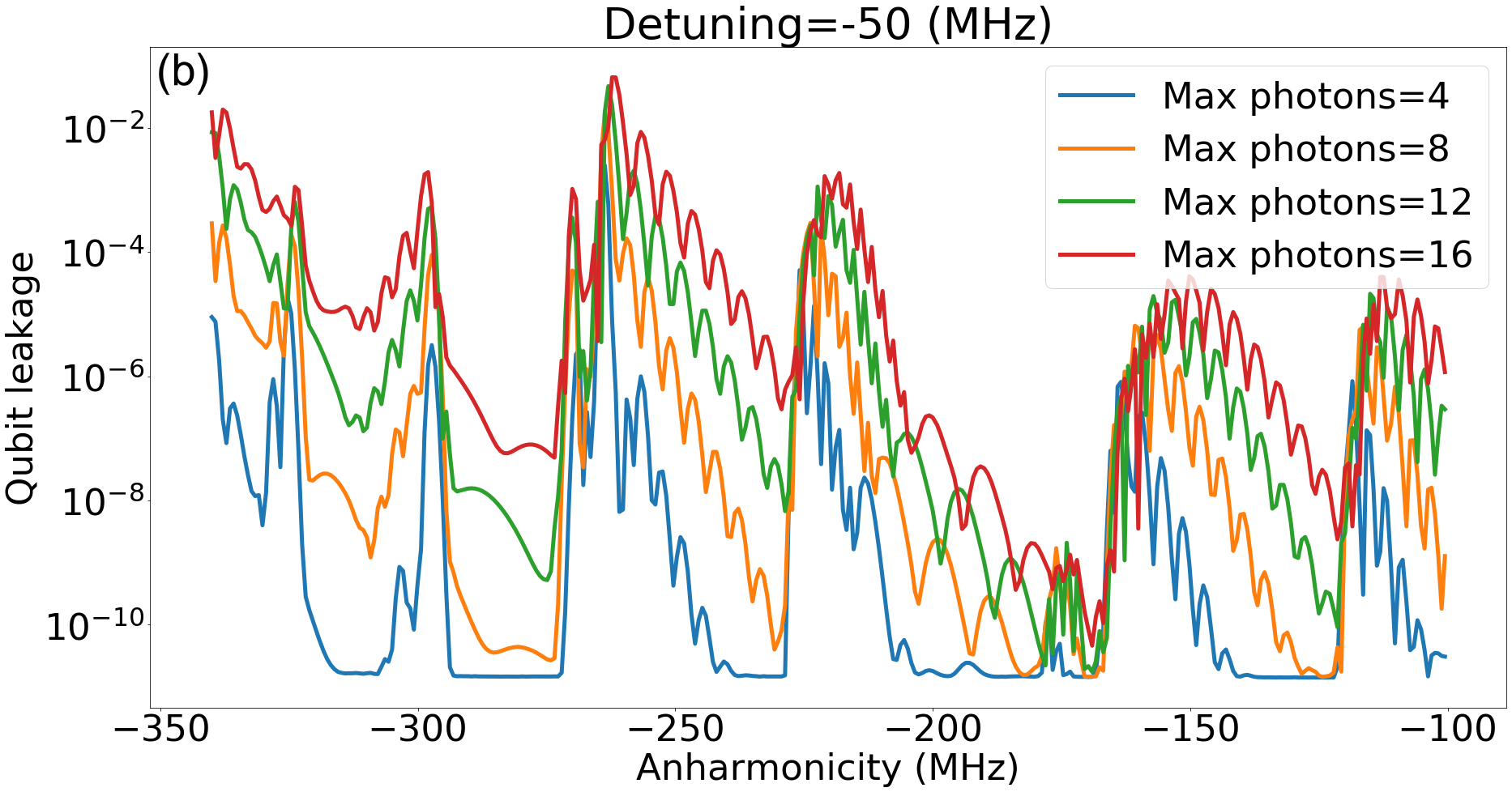
Figure 6: Qubit-resonator case — (a) Resonator leakage, (b) qubit leakage for the same parameters as in Fig. 5, constant detuning $\Delta_{cd}/2\pi=-50$ MHz and varying photon number.

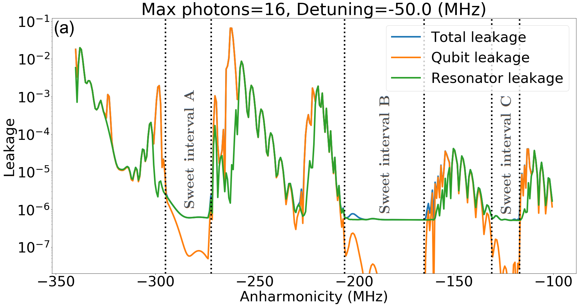
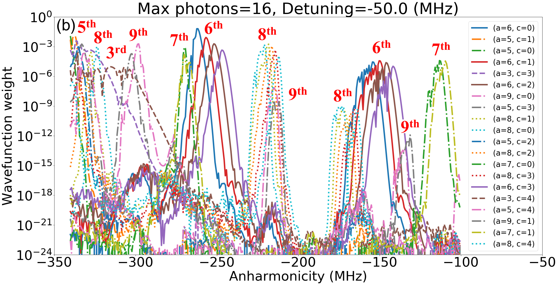
Figure 7: Qubit-resonator case — (a) Resonator, qubit and total leakage, (b) decomposition of leakage into qubit$\otimes$resonator eigenstates for the same parameters as in Fig. 6 and 16 maximum photons. The dominant leakage clusters in (b) correspond to specific high-excitation qubit states and variant photon number. They can be understood in terms of the frequency collisions in Fig. 8 and Table 1.

IV.1 Qubit-resonator leakage

We first consider a single transmon qubit coupled to a driven resonator which serves as a simpler version of the RIP gate that exhibits the essential leakage mechanisms for the qubit-resonator category. In particular, we observe leakage clusters to certain high-excitation qubit states and associate them with collisions between high-excitation and computational states of the qubit with different photon number. This analysis has implications beyond the RIP gate and specifically for optimal design of qubit readout. Similar drive-induced collisions have been studied in Ref. Sank_Measurement-Induced_2016 . Here, by sweeping qubit parameters, we categorize a series of collisions that extends Ref. Sank_Measurement-Induced_2016 (see Table 1).

For numerical simulation of the qubit-resonator case, we adopt the exact ab-initio Hamiltonian (1a)–(1b) with just one transmon qubit. To correctly model leakage to high-excitation states, we keep 10 transmon and 48 resonator eigenstates. The technical details of the numerical simulations are described in Appendix J. For experimentally relevant comparisons, we numerically search for the ab-initio system parameters in Eqs. (1a)–(1b) that keep certain relevant quantities fixed, while sweeping others. Given that the ab-initio and the pulse parameter space is large [8D (12D) for the single (two) qubit cases], our results are presented in terms of continuous sweeps only in select quantities such as qubit anharmonicity and resonator-drive detuning, with approximately constant cuts in other quantities such as the qubit frequency, resonator frequency, resonator photon number and dispersive shift.

We drive the resonator with the pulse shape

$$P_{\text{nc}}(t;\tau)\equiv\frac{1}{2}\left\{\cos\left[\pi\cos\left(\pi\frac{t}{\tau}\right)\right]+1\right\}\;,$$ (21)

which we call a nested cosine of duration $\tau$. Compared to a Gaussian pulse, the nested cosine pulse leads to improved resonator leakage due to smoother ramps Cross_Optimized_2015 (see Appendix E). We then compute the overall leakage as the residual occupation of system states at the end of the pulse. More specifically, resonator leakage is computed as the probability of finding the system with a non-zero photon number summed over all possible qubit states, and qubit leakage is found as the probability of finding the qubit outside the computational subspace summed over all possible resonator states.

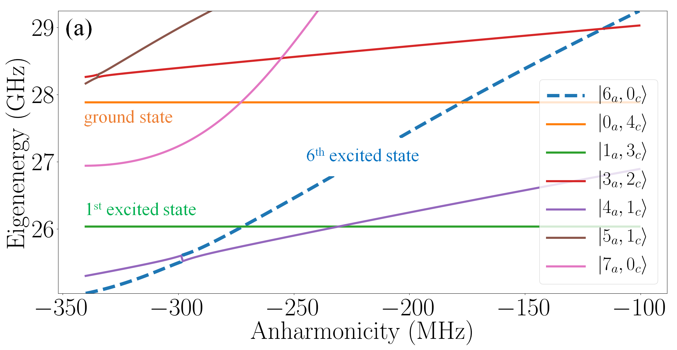
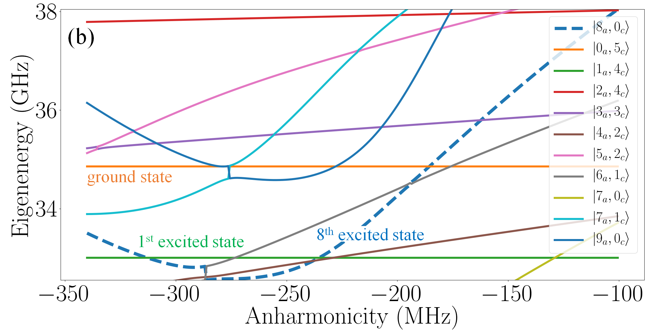
Figure 8: Qubit-resonator case — Examples of collisions between high-excitation and computational states for the same system parameters as in Figs. 6–7 without drive. States are labeled by the maximum overlap with the corresponding uncoupled case, hence avoided crossings appear as fictitious jumps. (a) Collisions between state $\ket{6_{a},0_{c}}$ and computational states $\ket{0_{a},4_{c}}$ (similar to Ref. Sank_Measurement-Induced_2016 ) and $\ket{1_{a},3_{c}}$. (b) Collisions between state $\ket{8_{a},0_{c}}$ and computational states $\ket{0_{a},5_{c}}$ and $\ket{1_{a},4_{c}}$. Note the possibility of multiple collisions between the same states due to e.g. bending of the 8th excited state at large anharmonicity [see Eq. (24)]. This is in agreement with observing two leakage clusters to the 6th excited state and three to the 8th excited state in Fig. 7(b).

We first analyze the case where the qubit and resonator frequencies are approximately fixed at $\omega_{a}/2\pi\approx 5140$ MHz and $\omega_{c}/2\pi\approx 6971$ MHz and the qubit-resonator dispersive coupling at $2\chi_{ac}/2\pi\approx-5.57$ MHz. Results for other qubit frequencies and dispersive shifts are also shown at the end of this section. Figure 5 shows the overall, resonator and qubit leakage for 16 photons as a 2D sweep of detuning and qubit anharmonicity, while comparing between pulses with and without DRAG to suppress drive at the resonator frequency. The DRAG pulse has the generic form

$$\Omega_{cy}(t)=\Omega_{c}P_{\text{nc}}(t;\tau)\;,$$ (22a)

$$\Omega_{cx}(t)=(1/\Delta_{D})\Omega_{c}\dot{P}_{\text{nc}}(t;\tau)\;.$$ (22b)

Setting the DRAG coefficient to $\Delta_{D}=\Delta_{cd}$ suppresses the pulse spectrum at the resonator-drive detuning (see Appendix E). This is confirmed in Fig. 5 where the background leakage is reduced by at least one order of magnitude at small $\Delta_{cd}$. Besides the resonator leakage at small $\Delta_{cd}$, there are leakage clusters as well as sweet intervals with suppressed leakage as a function of qubit anharmonicity. We observe that qubit-resonator leakage amplitude is generally suppressed at smaller qubit anharmonicity. This is understood as nonlinear interactions connecting the underlying states that increase in powers of $E_{C}$. For the chosen parameters, in particular, setting the detuning to be larger than 30 MHz and anharmonicity smaller than -200 MHz keeps leakage below the desired threshold of $10^{-5}$.

Figure 6 shows the resonator and the qubit leakage for constant detuning $\Delta_{cd}/2\pi\approx-50$ MHz and varying resonator photon number. Both types of leakage are universally increased at stronger drive. A decomposition of the overall leakage in terms of individual system states in Fig. 7 reveals that the dominant clusters can be associated with specific high-excitation qubit states and variant photon number. In particular, we observe considerable leakage to the 5th–9th excited states of the transmon qubit. Furthermore, clusters to a particular high-excitation qubit state can appear multiple times (twice for the 6th and 7th and three times for the 8th and 9th).

States	Condition (Kerr)	Kerr estimate of $\alpha_{a}/2\pi$ (MHz)	Numerical estimate of $\alpha_{a}/2\pi$ (MHz)
$\ket{5_{a},n_{c}}\sim\ket{0_{a},n_{c}+3}$	$5\omega_{a}+10\alpha_{a}\approx 3\omega_{c}-10n_{c}\chi_{ac}$	$-478.700+2.785n_{c}$	$-355.213+0.609n_{c}$
$\ket{6_{a},n_{c}}\sim\ket{0_{a},n_{c}+4}$	$6\omega_{a}+15\alpha_{a}\approx 4\omega_{c}-12n_{c}\chi_{ac}$	$-197.067+2.228n_{c}$	$-177.230+1.292n_{c}$
$\ket{6_{a},n_{c}}\sim\ket{1_{a},n_{c}+3}$	$5\omega_{a}+15\alpha_{a}\approx 3\omega_{c}-2(5n_{c}-3)\chi_{ac}$	$-320.247+1.857n_{c}$	$-272.136-0.981n_{c}$
$\ket{7_{a},n_{c}}\sim\ket{0_{a},n_{c}+4}$	$7\omega_{a}+21\alpha_{a}\approx 4\omega_{c}-14n_{c}\chi_{ac}$	$-385.524+1.857n_{c}$	$-272.892-0.423n_{c}$
$\ket{7_{a},n_{c}}\sim\ket{1_{a},n_{c}+4}$	$6\omega_{a}+21\alpha_{a}\approx 4\omega_{c}-4(3n_{c}-2)\chi_{ac}$	$-141.823+1.591n_{c}$	$-129.007+0.868n_{c}$
$\ket{8_{a},n_{c}}\sim\ket{0_{a},n_{c}+5}$	$8\omega_{a}+28\alpha_{a}\approx 5\omega_{c}-16n_{c}\chi_{ac}$	$-223.750+1.591n_{c}$	$-185.549+0.853n_{c}$
$\ket{8_{a},n_{c}}\sim\ket{1_{a},n_{c}+4}$	$7\omega_{a}+28\alpha_{a}\approx 4\omega_{c}-2(7n_{c}-4)\chi_{ac}$	$-289.939+1.393n_{c}$	$-235.336+1.096n_{c}$ $\bullet-313.738+708n_{c}$
$\ket{9_{a},n_{c}}\sim\ket{0_{a},n_{c}+5}$	$9\omega_{a}+36\alpha_{a}\approx 5\omega_{c}-18n_{c}\chi_{ac}$	$-316.806+1.393n_{c}$	$-227.839+0.807n_{c}$ $\bullet-280.415+1.549n_{c}$
$\ket{9_{a},n_{c}}\sim\ket{1_{a},n_{c}+5}$	$8\omega_{a}+36\alpha_{a}\approx 5\omega_{c}-2(8n_{c}-5)\chi_{ac}$	$-174.801+1.238n_{c}$	$-147.268+1.549n_{c}$

Table 1: Examples of qubit-resonator frequency collisions between the high-excitation and computational subspaces observed in Figs. 5–7. The leftmost column shows the colliding quantum states (qubit $\otimes$ resonator), the second provides a collision condition based on the undriven Kerr spectrum, and the third and the fourth provide experimental estimates for qubit anharmonicity assuming the same parameters as in Figs. 6 and 7 and based on Kerr and exact ab-initio models, respectively. The Kerr model approximately captures the order by which these clusters happen, but the estimate is less valid especially for collisions involving higher qubit states and occurring at larger anharmonicity. In particular, the ab-initio analysis reveals the possibility of additional collisions between the same states [shown with a bullet, see e.g. Fig. 8(b)].

Analytical modeling of leakage requires advanced time-dependent methods such as SWPT or Magnus expansion Magnus_Exponential_1954 ; Blanes_Magnus_2009 ; Blanes_Pedagogical_2010 . It is in principle possible to use time-dependent SWPT to compute leakage rates. However, generally, SWPT is more suitable for computing effective (resonant) rates, while leakage rates are more easily found via Magnus. For the RIP gate, the two methods are connected via

$$\hat{U}_{I}(t,0)=\hat{U}_{\text{diag}}(t)\hat{U}_{I,\text{eff}}(t,0)\hat{U}^{{\dagger}}_{\text{diag}}(0)\;,$$ (23)

where $\hat{U}_{I}(t,0)$ and $\hat{U}_{I,\text{eff}}(t,0)$ are the overall and the effective time-evolution operators, and $\hat{U}_{\text{diag}}(t)$ is the mapping similar to Eq. (8). For a physical process to cause leakage, it must be off-diagonal with respect to the computational eigenstates. Hence, in SWPT, the information about leakage is encoded indirectly through $\hat{U}_{\text{diag}}(t)$. In Magnus, however, we perform an expansion directly on $\hat{U}_{I}(t,0)$ (see Appendix H).

Regardless of the method, the contribution from each physical process appears as the Fourier transform of the underlying time-dependent interaction rate evaluated at the corresponding system transition frequency. Therefore, leakage can be characterized given the following information: (i) system transition frequencies, (ii) interaction matrix elements (connectivity between the eigenstates), and (iii) spectral content of the interaction (pulse shape). Once the pulse spectrum has a non-negligible overlap with a particular system transition frequency, we expect an increase in the leakage. Even though capturing the precise leakage amplitude is a difficult task, estimating where leakage occurs in the parameter space is feasible based on the frequency collisions in the system spectrum.

Consequently, regions in system parameter space where a computational state becomes degenerate with a high-excitation qubit state provide a bridge for leakage given that such states are connected directly or indirectly by the underlying interaction. Figure 8 provides two examples of such collisions as a function of qubit anharmonicity. Firstly, state $\ket{6_{a},0_{c}}$ collides with states $\ket{0_{a},4_{c}}$ and $\ket{1_{a},3_{c}}$ at $\alpha_{a}/2\pi\approx-177.230$ MHz and $\alpha_{a}/2\pi\approx-272.136$ MHz, respectively, explaining the two observed leakage clusters in Fig. 7(b). The clustering is due to additional collisions with increasing photon number, e.g. between $\ket{6_{a},1_{c}}$ and $\ket{0_{a},5_{c}}$ etc (see Table 1). Secondly, state $\ket{8_{a},0_{c}}$ collides once with state $\ket{0_{a},5_{c}}$ at $\alpha_{a}/2\pi\approx-185.549$ MHz and twice with state $\ket{1_{a},4_{c}}$ at $\alpha_{a}/2\pi\approx-235.336$ MHz and $\alpha_{a}/2\pi\approx-313.738$ MHz, in agreement with the three leakage clusters in Fig. 7(b). Such repeated collisions between the same states cannot be predicted by the Kerr model which is linear in qubit anharmonicity. It is a signature that the sextic, and possibly higher order, expansion of the Josephson potential is relevant at larger anharmonicity as (assuming $g_{a}=0$ and $n_{ga}=0$)

$$\begin{split}\hat{\mathcal{H}}_{qa}&=(8E_{Ca}E_{Ja})^{1/2}\hat{a}^{{\dagger}}\hat{a}-\frac{E_{Ca}}{12}\left(\hat{a}+\hat{a}^{{\dagger}}\right)^{4}\\ &+\frac{(2E_{Ca}^{3}/E_{Ja})^{1/2}}{360}\left(\hat{a}+\hat{a}^{{\dagger}}\right)^{6}+O\left(\frac{E_{Ca}^{2}}{E_{Ja}}\right)\;.\end{split}$$ (24)

Moreover, the observation that the high- and low-excitation qubit states cross, as opposed to undergoing an anti-crossing, reveals that such states are not coupled via nonlinearity but rather through an unwanted projection of the RIP drive over the corresponding transition. A summary of the observed qubit-resonator collisions as well as a comparison between ab-initio and Kerr predictions is given in Table 1.

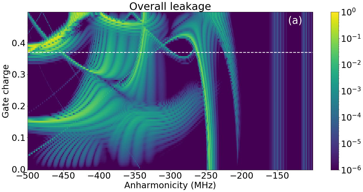
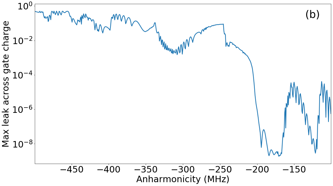
Figure 9: Qubit-resonator case — Dependence of overall leakage with DRAG on the gate charge for the same parameters as in Fig. 6, resonator-drive detuning set to -50 MHz, and maximum photon number set to 16. (a) 2D sweep of overall leakage as a function of gate charge and anharmonicity. The result is approximately periodic and symmetric under change of sign for the gate charge, hence the approximately unique interval of [0,0.5] is shown. The white dashed line shows the value of gate charge at 0.37 used in Figs. 5–8. (b) Maximum overall leakage across the gate charge, which accounts for the worst case scenario at each anharmonicity value.

Given the correspondence between qubit-resonator leakage clusters and frequency collisions involving high-excitation qubit states, it is also crucial to quantify and optimize the dependence of leakage on gate charge for two main reasons. Firstly, higher-excitation eigenenergies of the transmon qubit depend more strongly on the gate charge Koch_Charge_2007 , causing non-negligible shifts of the leakage clusters in the parameter space. Secondly, and more importantly, the gate charge is neither controllable nor predictable in the experiment. A more realistic measure is then the maximum leakage over one period of gate charge for each parameter set. Figure 9 shows the dependence of qubit-resonator overall leakage on the qubit anharmonicity and the gate charge, over the approximately unique interval of $n_{ga}\in[0,0.5]$ . We observe that smaller anharmonicity, approximately below -200 MHz, leads to significantly less leakage cluster density, less leakage amplitude and less dependence of leakage on the gate charge.

The results so far were based on fixed $\omega_{a}/2\pi\approx 5140$, $\omega_{c}/2\pi\approx 6971$ and $2\chi_{ac}/2\pi\approx-5.57$ MHz. According to Table 1, the collision conditions depend also strongly on these parameters. In particular, if the qubit frequency is increased, there is less chance of qubit-resonator collisions in the anharmonicity range relevant for experiment. For instance, consider the $\ket{6_{a},0_{c}}\sim\ket{1_{a},3_{c}}$ collision, with approximate Kerr condition $6\omega_{a}+15\alpha_{a}\approx\omega_{a}+3\omega_{c}+6\chi_{ac}$. Setting $\omega_{a}/2\pi\approx 6000$ MHz, keeping other parameters the same, pushes the collision to $\alpha_{a}/2\pi\approx-606.914$ MHz, away from the transmon regime. This behavior holds for qubit-resonator collisions in general. Moreover, the dispersive shift $2\chi_{ac}$ determines the number-splitting span in each cluster. Hence there is a trade-off between large $2\chi_{ac}$, desired for large dynamic $ZZ$, and the width of collision-free anharmonicity intervals. Figure 10 compares the qubit-resonator leakage of three distinct qubit frequencies $\omega_{a}/2\pi\approx 4750$, $5140$, $6000$ MHz and two dispersive shifts $2\chi_{ac}/2\pi\approx-5.57$, $-2.79$ MHz, and confirms the above-mentioned trends. Importantly, based on Figs. 10(e)–10(f), working with the 6000 MHz frequency qubit removes most of the leakage clusters from the considered anharmonicity range and mitigates the amplitude of the remaining ones.

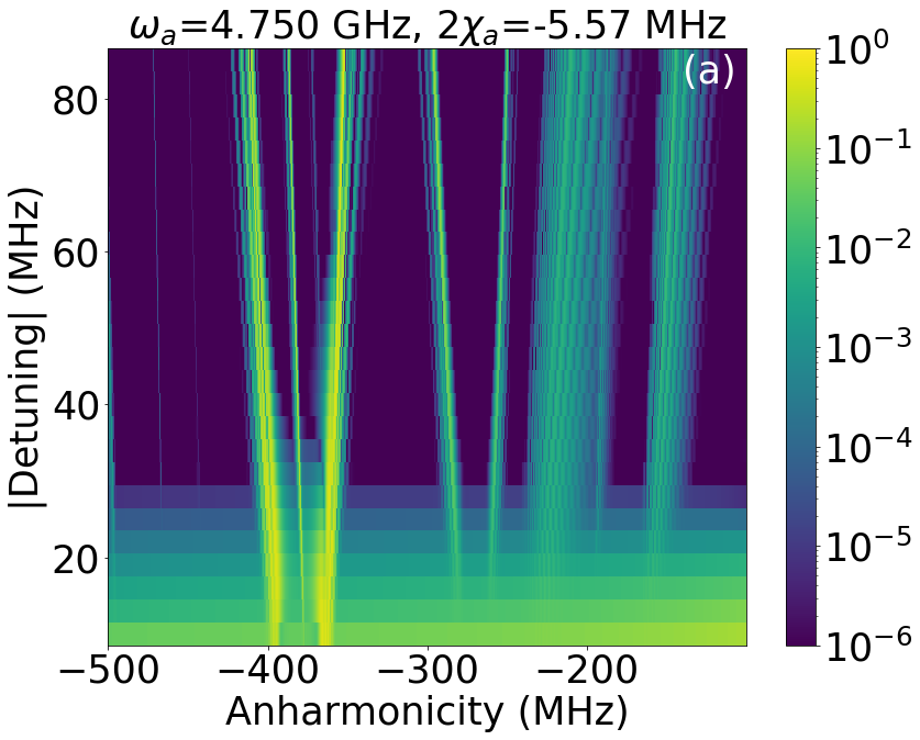
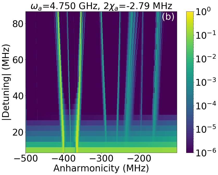
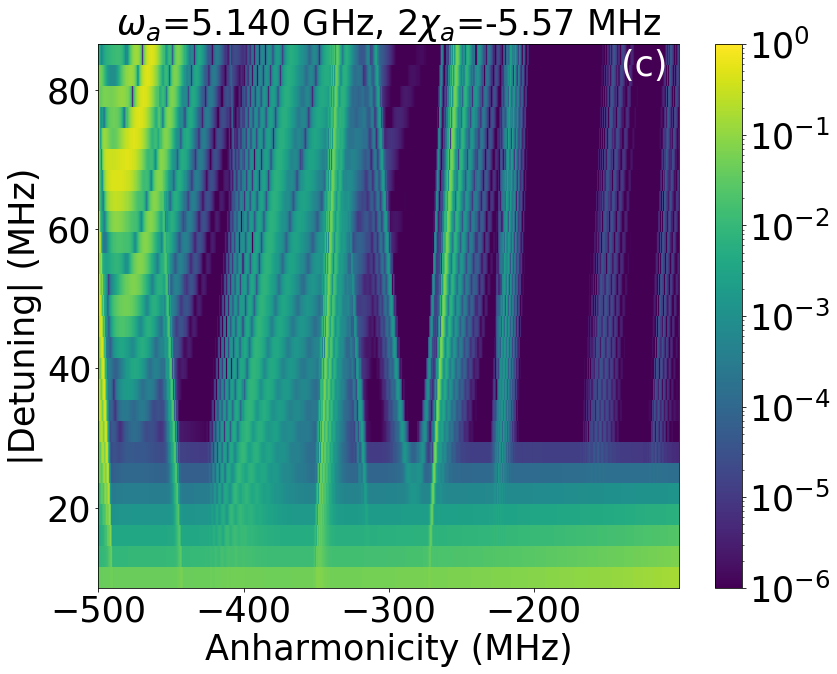
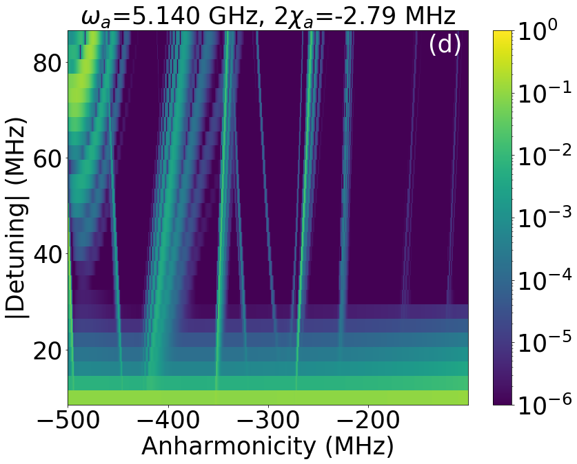
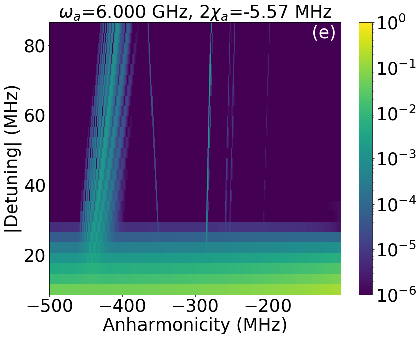
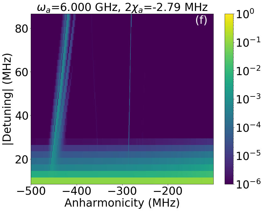
Figure 10: Qubit-resonator case — Overall leakage with DRAG for three different qubit frequencies $\omega_{a}/2\pi\approx 4750$ [(a), (b)], $5140$ [(c), (d)], $6000$ [(e), (f)] MHz, and two distinct dispersive shifts $2\chi_{ac}/2\pi\approx-5.57$ MHz (left column) and $-2.79$ MHz (right column), with maximum photon number set to 16. Other parameters are the same as Fig. 5.

IV.2 Three-body leakage

The main physics of qubit-resonator collisions and leakage can in principle be extended to understand more complex three-body collisions. Compared to the qubit-resonator case, which results in leakage to relatively high-excitation qubit states (5th–9th), having both qubits participating in exchange interactions allows for leakage to low-excitation qubit states as well. For instance, a single excitation of the low-frequency qubit and one resonator photon can provide the energy to leak to the 2nd excited state of the high-frequency qubit, i.e. a collision of the form $\ket{1_{a},0_{b},1_{c}}\sim\ket{0_{a},2_{b},0_{c}}$. For example, this collision can be satisfied if $\omega_{a}/2\pi\approx 4750$, $\omega_{b}/2\pi\approx 6000$, $\omega_{c}/2\pi\approx 6971$ and $\alpha_{b}/2\pi\approx-279$ MHz. We refer to this frequency configuration as the high-low RIP pair.

States	Condition (Kerr)	Instance
$\ket{3_{a},0_{b},n_{c}}\sim\ket{0_{a},1_{b},n_{c}+1}$	$3\omega_{a}+3\alpha_{a}+6n_{c}\chi_{ac}\approx\omega_{b}+\omega_{c}+2(n_{c}+1)\chi_{bc}$	high-low
$\ket{4_{a},0_{b},n_{c}}\sim\ket{0_{a},1_{b},n_{c}+2}$	$4\omega_{a}+6\alpha_{a}+8n_{c}\chi_{ac}\approx\omega_{b}+2\omega_{c}+2(n_{c}+2)\chi_{bc}$	high-high
$\ket{5_{a},0_{b},n_{c}}\sim\ket{0_{a},1_{b},n_{c}+2}$	$5\omega_{a}+10\alpha_{a}+10n_{c}\chi_{ac}\approx\omega_{b}+2\omega_{c}+2(n_{c}+2)\chi_{bc}$	high-low
$\ket{5_{a},0_{b},n_{c}}\sim\ket{1_{a},1_{b},n_{c}+1}$	$4\omega_{a}+10\alpha_{a}+10n_{c}\chi_{ac}\approx\omega_{b}+\omega_{c}+2(n_{c}+1)(\chi_{ac}+\chi_{bc})$	high-low
$\ket{6_{a},0_{b},n_{c}}\sim\ket{1_{a},1_{b},n_{c}+2}$	$5\omega_{a}+15\alpha_{a}+12n_{c}\chi_{ac}\approx\omega_{b}+2\omega_{c}+2(n_{c}+2)(\chi_{ac}+\chi_{bc})$	high-low
$\ket{7_{a},0_{b},n_{c}}\sim\ket{1_{a},1_{b},n_{c}+2}$	$6\omega_{a}+21\alpha_{a}+14n_{c}\chi_{ac}\approx\omega_{b}+2\omega_{c}+2(n_{c}+2)(\chi_{ac}+\chi_{bc})$	high-low
$\ket{7_{a},0_{b},n_{c}}\sim\ket{1_{a},1_{b},n_{c}+3}$	$6\omega_{a}+21\alpha_{a}+14n_{c}\chi_{ac}\approx\omega_{b}+3\omega_{c}+2(n_{c}+3)(\chi_{ac}+\chi_{bc})$	high-high
$\ket{8_{a},0_{b},n_{c}}\sim\ket{1_{a},1_{b},n_{c}+2}$	$7\omega_{a}+28\alpha_{a}+16n_{c}\chi_{ac}\approx\omega_{b}+2\omega_{c}+2(n_{c}+2)(\chi_{ac}+\chi_{bc})$	high-low
$\ket{0_{a},2_{b},n_{c}}\sim\ket{1_{a},0_{b},n_{c}+1}$	$2\omega_{b}+\alpha_{b}+4n_{c}\chi_{bc}\approx\omega_{a}+\omega_{c}+2(n_{c}+1)\chi_{ac}$	high-low
$\ket{0_{a},5_{b},n_{c}}\sim\ket{1_{a},1_{b},n_{c}+2}$	$4\omega_{b}+10\alpha_{b}+10n_{c}\chi_{bc}\approx\omega_{a}+2\omega_{c}+2(n_{c}+2)(\chi_{ac}+\chi_{bc})$	high-high
$\ket{0_{a},7_{b},n_{c}}\sim\ket{1_{a},1_{b},n_{c}+3}$	$6\omega_{b}+21\alpha_{b}+14n_{c}\chi_{bc}\approx\omega_{a}+3\omega_{c}+2(n_{c}+3)(\chi_{ac}+\chi_{bc})$	high-high
$\ket{2_{a},3_{b},n_{c}}\sim\ket{1_{a},0_{b},n_{c}+3}$	$\omega_{a}+\alpha_{a}+3\omega_{b}+3\alpha_{b}+4n_{c}\chi_{ac}+6n_{c}\chi_{bc}\approx 3\omega_{c}+2(n_{c}+3)\chi_{ac}$	high-low
$\ket{2_{a},5_{b},n_{c}}\sim\ket{1_{a},0_{b},n_{c}+4}$	$\omega_{a}+\alpha_{a}+5\omega_{b}+10\alpha_{b}+4n_{c}\chi_{ac}+10n_{c}\chi_{bc}\approx 4\omega_{c}+2(n_{c}+4)\chi_{ac}$	high-low
$\ket{3_{a},1_{b},n_{c}}\sim\ket{1_{a},0_{b},n_{c}+2}$	$2\omega_{a}+3\alpha_{a}+\omega_{b}+6n_{c}\chi_{ac}+2n_{c}\chi_{bc}\approx 2\omega_{c}+2(n_{c}+2)\chi_{ac}$	high-low
$\ket{3_{a},2_{b},n_{c}}\sim\ket{1_{a},1_{b},n_{c}+2}$	$2\omega_{a}+3\alpha_{a}+\omega_{b}+\alpha_{b}+6n_{c}\chi_{ac}+4n_{c}\chi_{bc}\approx 2\omega_{c}+2(n_{c}+2)(\chi_{ac}+\chi_{bc})$	high-low
$\ket{5_{a},2_{b},n_{c}}\sim\ket{1_{a},1_{b},n_{c}+3}$	$4\omega_{a}+10\alpha_{a}+\omega_{b}+\alpha_{b}+10n_{c}\chi_{ac}+4n_{c}\chi_{bc}\approx 3\omega_{c}+2(n_{c}+3)(\chi_{ac}+\chi_{bc})$	high-low

Table 2: Examples of dominant three-body collisions observed in Figs. 11–12. The first column describes the colliding states, the second provides an approximate collision condition based on the Kerr model, and the last column shows in which frequency configuration the collision was observed. The list here is derived from Figs. 11–12 with a leakage cut-off of $10^{-5}$ for each collision assuming 4 maximum resonator photons. In principle, however, there are numerous possibilities.

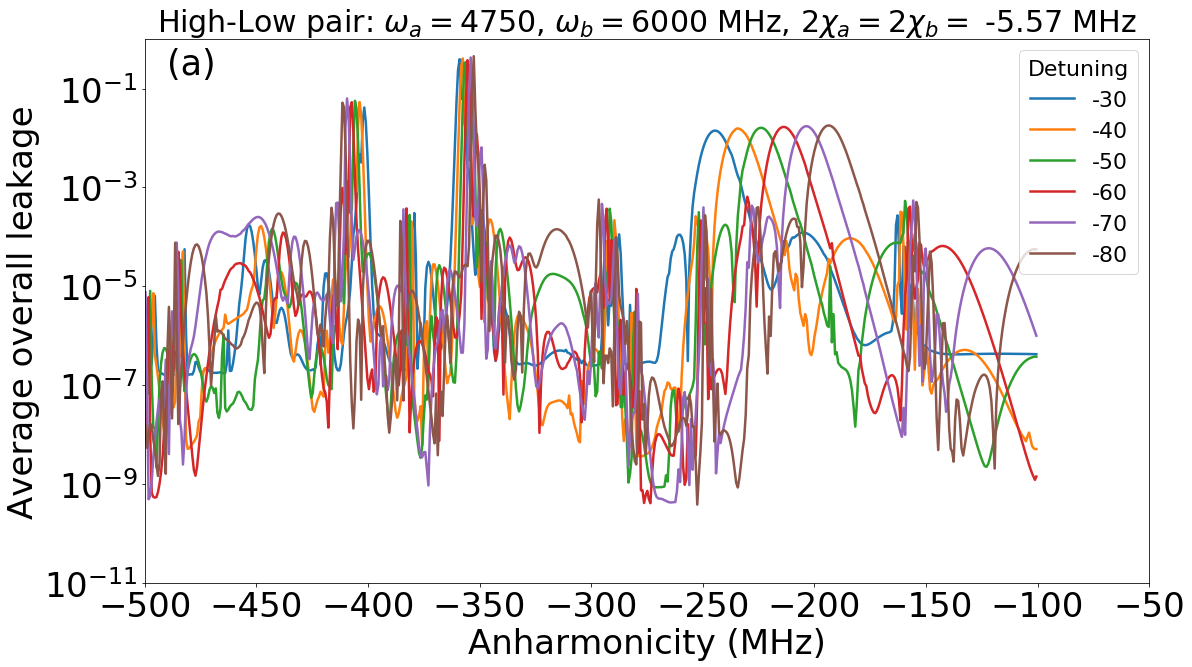
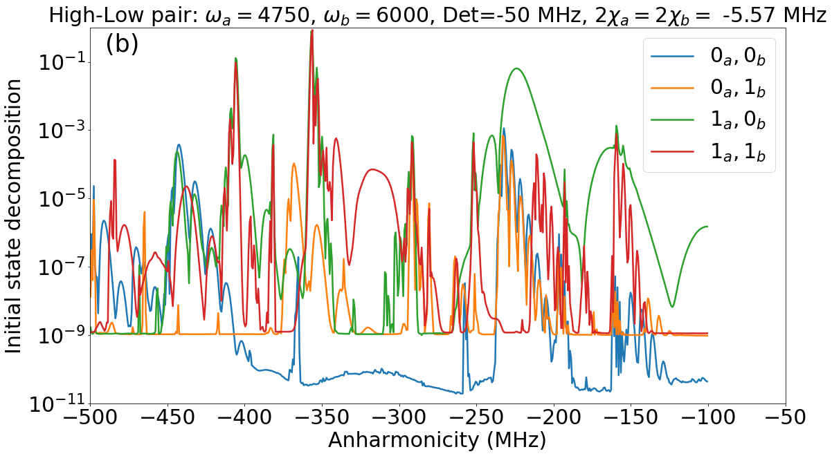
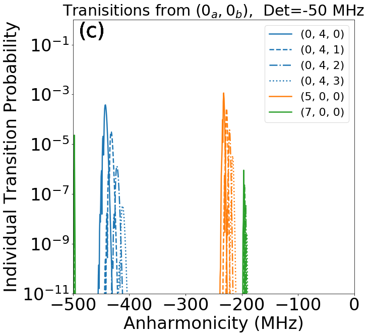
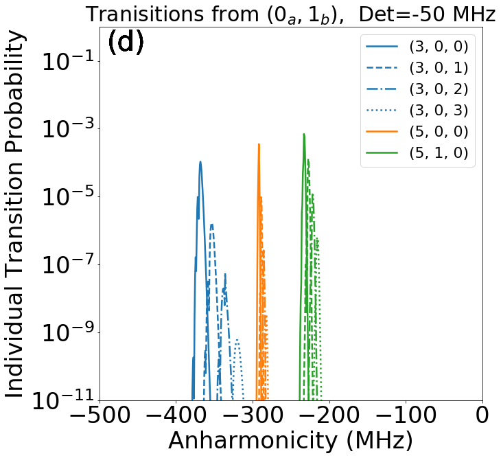
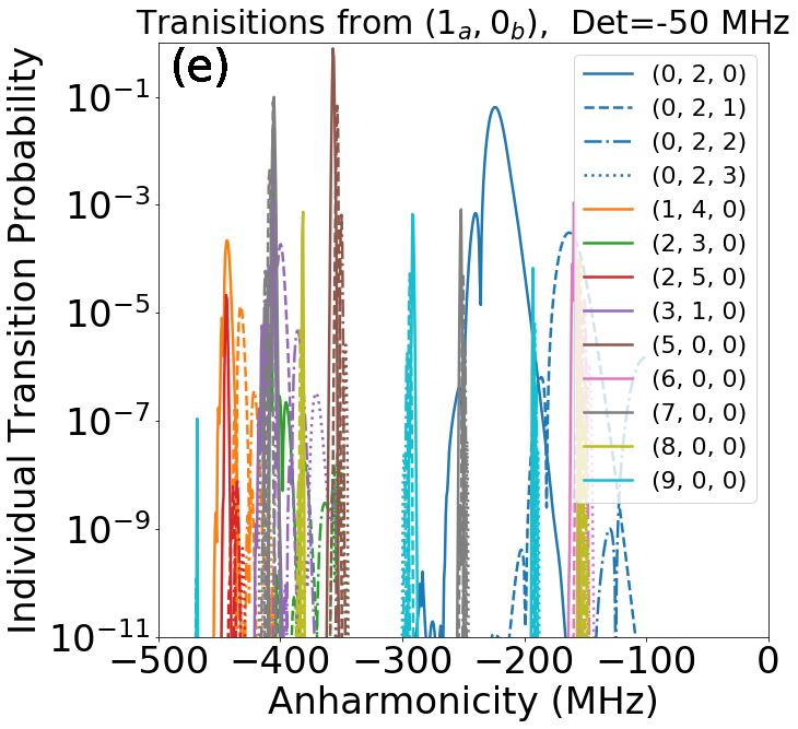
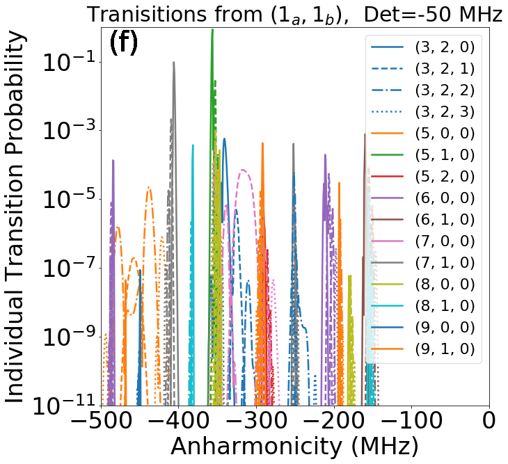
Figure 11: Two-qubit simulation of leakage for the high-low pair with $\omega_{a}/2\pi\approx 4750$, $\omega_{b}/2\pi\approx 6000$, $\omega_{c}/2\pi\approx 6971$, $2\chi_{ac}/2\pi\approx 2\chi_{bc}/2\pi\approx-5.57$ MHz using a $200$ ns nested cosine pulse equivalent to 4 photons at the pulse maximum. (a) Overall leakage with DRAG, averaged over the four initial two-qubit states, $\ket{0_{a},0_{b},0_{c}}$, $\ket{0_{a},1_{b},0_{c}}$, $\ket{1_{a},0_{b},0_{c}}$ and $\ket{1_{a},1_{b},0_{c}}$, as a function of $\alpha_{a}\approx\alpha_{b}$ and $\Delta_{cd}$. (b) Overall leakage for each initial computational state at fixed $\Delta_{cd}/2\pi=-50$ MHz. (c)–(f) Individual leakage transition probabilities starting from the four computational states, respectively. Compared to the qubit-resonator simulations of Sec. IV.1, 10 energy eigenstates and 22 resonator states are kept.

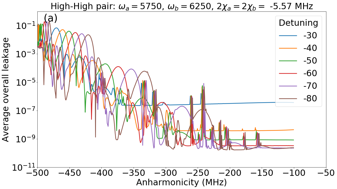
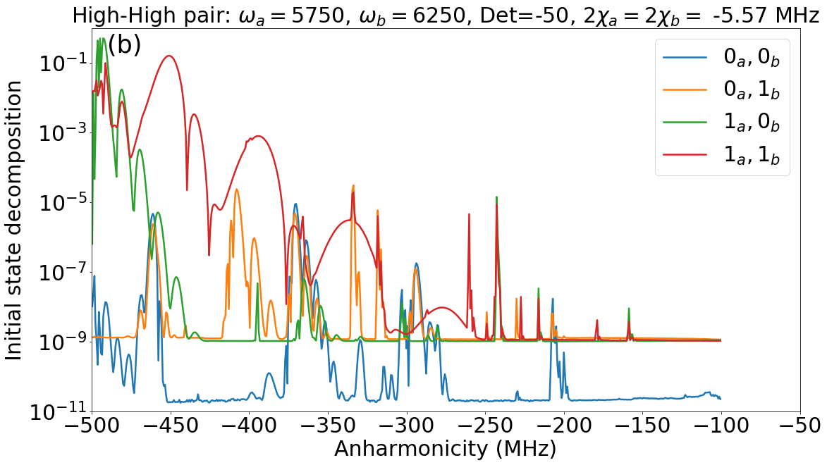
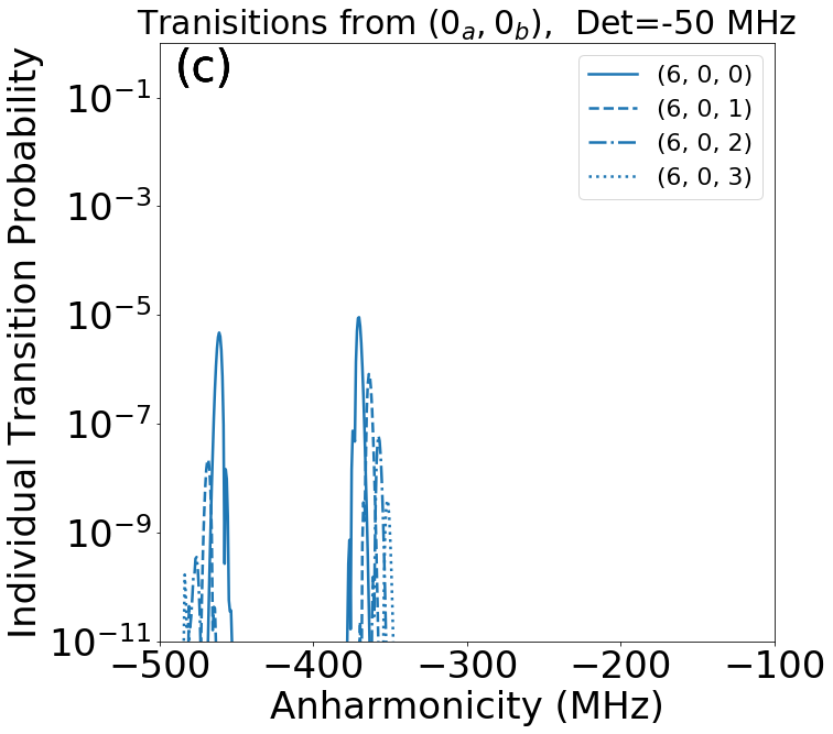
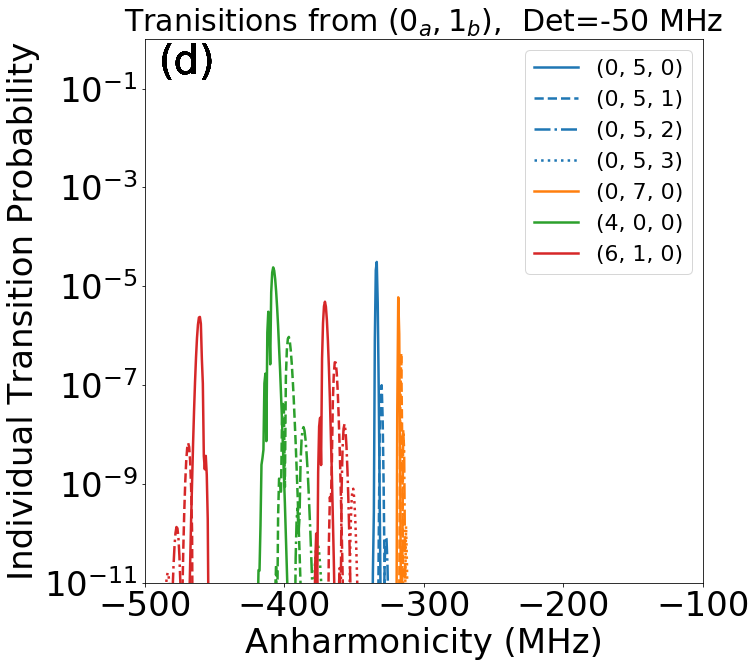
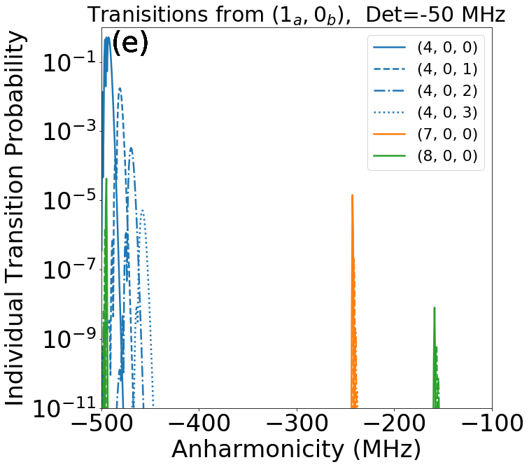
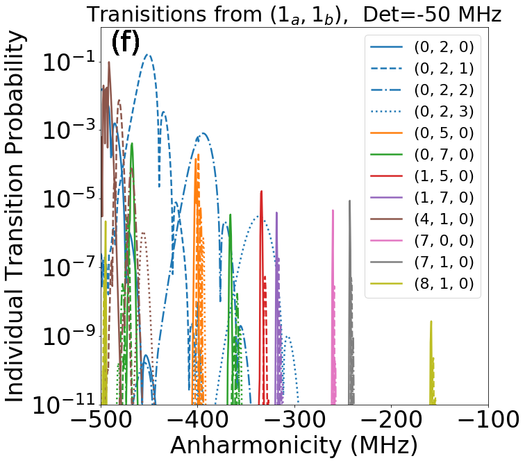
Figure 12: Two-qubit simulation of leakage for the high-high pair with $\omega_{a}/2\pi\approx 5750$, $\omega_{b}/2\pi\approx 6250$ MHz and other parameters the same as Fig. 11. Compared to the high-low configuration, we observe a significant suppression of leakage especially for $\alpha_{a}/2\pi\approx\alpha_{b}/2\pi\lessapprox-200$ MHz.

We then compare the high-low configuration given above to an improved RIP pair. Based on the preceding discussion of qubit-resonator leakage (Sec. IV.1 and Fig. 10), both qubit frequencies should be set as close to the resonator frequency as is allowed by other constraints on the parameters. As one of the advantages of the RIP gate is a wider range of allowed qubit frequency values, we choose to keep the qubits outside of the straddling regime. When qubits are designed to operate in the straddling regime, the design, subject to sample-to-sample variation in fabrication, is more susceptible to qubit-qubit collisions of the form $\ket{1_{a},1_{b},n_{c}}\sim\ket{2_{a},0_{b},n_{c}}$ and $\ket{1_{a},1_{b},n_{c}}\sim\ket{0_{a},2_{b},n_{c}}$, with approximate collision conditions $\Delta_{ab}\approx\alpha_{b}$ and $\Delta_{ab}\approx-\alpha_{a}$. Moreover, since our model does not include a cancellation coupler, small qubit-qubit detuning leads to a large static $ZZ$, reducing the on/off ratio of the RIP gate. Therefore, as a contrast to the high-low configuration given above, we pick a second “high-high” configuration with $\omega_{a}/2\pi\approx 5750$, $\omega_{b}/2\pi\approx 6250$, and $\omega_{c}/2\pi\approx 6971$ MHz, corresponding to a $500$ MHz qubit-qubit detuning. We find that the high-high pair reduces three-body leakage compared to the high-low configuration while also having low qubit-resonator leakage.

For the two-qubit simulation, the ab-initio system parameters were selected to produce the qubit and resonator frequency values of the high-high and high-low scenarios while fixing qubit-resonator dispersive shifts at $2\chi_{ac}/2\pi\approx 2\chi_{bc}/2\pi\approx-5.57$ MHz. Such parameters were found for a range of qubit anharmonicities from -500 to -100 MHz, with the anharmonicity of the two qubits kept approximately equal, $\alpha_{a}\approx\alpha_{b}$, for each case. The pulse parameters were set to produce a maximum resonator photon number of 4 over multiple traces of constant resonator-drive detuning. Compared to the single-qubit simulations of Sec. IV.1, these simulations used 22 resonator states and 10 energy eigenstates for each qubit.

Figures 11 and 12 provide the leakage analysis for the high-low and high-high RIP pairs, respectively. We note that in such two-qubit simulations all leakage categories, as described in Fig. 4, can be driven in principle. Therefore, to better understand each case, the observed leakage peaks in panel (a) are decomposed into separate transitions in terms of initial computational states in panel (b) and final leaked states in panels (c)–(f). We find that the high-high allocation produces regions of overall leakage below $10^{-6}$ especially at weak qubit anharmonicity less than -200 MHz. However, for the high-low case, the clusters are spread over the considered anharmonicity range and no discernible suppression is observed at weaker anharmonicity. This is in part due to the strong qubit-resonator collisions for the low-frequency qubit as also observed in Fig. 10(a), but decomposition of leakage into individual transitions in panels (c)–(f) also reveals a series of three-body leakage transitions in which both qubits participate in the excitation exchange. In particular, the high-low case suffers from both higher three-body leakage cluster density and stronger peaks compared to the high-high case. Table 2 provides examples of dominant three-body collisions corresponding to the two cases. For example, below -250 MHz anharmonicity, the dominant leakage transitions for the high-low case satisfy $\ket{0_{a},2_{b},n_{c}}\sim\ket{1_{a},0_{b},n_{c}+1}$.

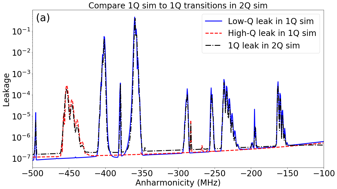
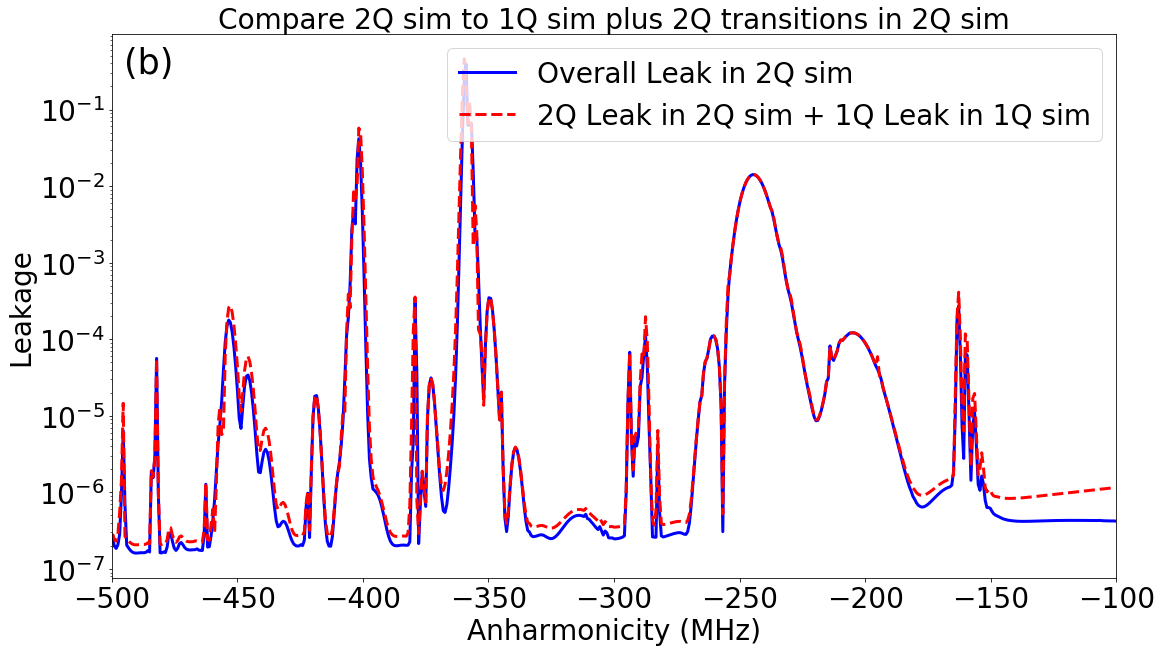
Figure 13: Comparison between single- and two-qubit simulations for the high-low pair with resonator-drive detuning set to -30 MHz and 4 maximum photons — (a) Individual qubit-resonator leakage for each qubit compared to the qubit-resonator leakage obtained from the two-qubit simulation. (b) Overall leakage obtained from the two-qubit simulation compared to the sum of qubit-resonator leakage obtained from the single-qubit simulation and three-body leakage obtained from the two-qubit simulation.

To validate our characterization of the RIP gate leakage in terms of distinct categories, we show that qubit-resonator leakage computed from the single-qubit simulation in Sec. IV.1 agrees well with the two-qubit simulation here. In particular, for the high-low pair, Fig. 13(a) demonstrates a good agreement between the qubit-resonator leakage from individual single-qubit simulations and the qubit-resonator leakage from the two-qubit simulation. Furthermore, Fig. 13(b) shows that adding the three-body leakage from the two-qubit simulation to the qubit-resonator leakage from separate single-qubit simulations recovers the overall leakage in the two-qubit simulation. For this analysis, the two-qubit simulation results were split into qubit-resonator and three-body leakage by looking at whether the final leaked state involved a transition of one or both of the qubits. These observations confirm that, when choosing system parameters to avoid RIP gate leakage, the different leakage categories can be considered independently, since the presence of the 2nd qubit does not noticeably change the nature of the single-qubit transitions.

In summary, our analysis of leakage has important implications in terms of optimal parameter allocation for the RIP gate. Although the background leakage can be controlled dynamically, i.e. through modifying $\omega_{d}$, $\tau$ and DRAG, the qubit-resonator and three-body leakage clusters result from ill-chosen static system parameters. It can be shown that average gate fidelity is limited by average leakage Wood_Quantification_2018 (see Appendix I). Therefore, improving fidelity requires suppressing leakage.

V Takeaways for control and design

In this section, we summarize our findings and provide a set of instructions for optimal parameter allocation. The discussion is based on the ab-initio model in Eqs. (1a)–(1b), for which there are 12 independent system and pulse parameters: $E_{Ca}$, $E_{Cb}$, $E_{Ja}$, $E_{Jb}$, $n_{ga}$, $n_{gb}$, $g_{a}$, $g_{b}$, $\omega_{c}$, $\omega_{d}$, $\Omega_{c}$ and $\tau$. The nested cosine pulse shape in Eq. (21) is fully characterized by the gate time $\tau$, while in principle there can be more pulse parameters. In what follows, we describe distinct interdependencies between certain subsets of parameters which need to be taken into account for RIP device design. In principle, these subsets are not completely independent; however, dissecting into simpler few-parameter dependencies facilitates the search. We sort the following conditions from the most to the least trivial as:

• Resonator frequency $\omega_{c}$ — The measurement equipment sets the choice for $\omega_{c}$ typically at 7000 MHz.

• Drive frequency $\omega_{d}$ and gate time $\tau$ — Driving above the resonator, i.e. $\omega_{d}>\omega_{c}$, leads to less background leakage, while for $\omega_{d}<\omega_{c}$ there is excessive leakage due to the other $2\chi$-shifted resonator poles [Fig. 2 and Eq. (16c)]. Pulse-resonator spectral overlap and the resulting background leakage is approximately determined by the product $\Delta_{cd}\tau$ (see Appendix E). The leakage clusters tend to fan out at larger detuning (Fig. 5), hence $\Delta_{cd}$ should be as small as allowed by the background leakage threshold. Filtering the pulse at $\Delta_{cd}$ in general, and applying DRAG in particular [Eqs. (22a)–(22b)], are beneficial in reducing $\Delta_{cd}$ for fixed leakage. Based on the simulation with DRAG, $|\Delta_{cd}/2\pi|\gtrapprox 30$ MHz is a reasonable choice for $\tau\approx 200$ ns.

• Charging energy $E_{C}$ and Josephson energy $E_{J}$ — Qubit frequency and anharmonicity are related to $E_{C}$ and $E_{J}$ up to $O(E_{C}^{2}/E_{J})$ as Koch_Charge_2007 ; Didier_Analytical_2018 (assuming $g=0$ and $n_{g}=0$)

  $$\quad\quad\omega\approx(8E_{J}E_{C})^{1/2}-E_{C}-\frac{1}{4}\left(\frac{2E_{C}}{E_{J}}\right)^{1/2}E_{C}\;,$$ (25a)

  $$\quad\quad\alpha\approx-E_{C}-\frac{9}{16}\left(\frac{2E_{C}}{E_{J}}\right)^{1/2}E_{C}\;.$$ (25b)

  A few observations are in order based in part on our simulation results. First, operating in the transmon limit reduces the set of possible collisions by reducing the dependence of the spectrum on the gate offset charge Koch_Charge_2007 . Second, both qubit-resonator and three-body leakage amplitude are universally reduced at smaller qubit anharmonicity [Figs. 5 and 12]. Third, smaller anharmonicity leads also to less eigenenergy crowding and collisions (compare collision density at -400 to -200 MHz in Fig. 5). Fourth, larger qubit frequency pushes the qubit-resonator collisions to occur at larger anharmonicity values outside the range relevant to experiment (less collisions for $\omega/2\pi\approx 6000$ MHz compared to $\omega/2\pi\approx 5140$ MHz in Fig. 10). All in all, it is beneficial to work with very weakly anharmonic qubits with sufficiently small anharmonicity, of the order of -200 MHz. With this choice, $\omega/2\pi\approx 5140$ and $6000$ MHz correspond to $E_{J}/E_{C}\approx 103.29$ and $136.71$, respectively. Lastly, we note that smaller anharmonicity, i.e. going from -340 MHz that is common for CR architectures to -200 MHz, can in principle enhance the $\ket{1_{a}}\rightarrow\ket{2_{a}}$ leakage during single-qubit gate operations. However, this is not a limiting factor, since single-qubit leakage can be mitigated via a combination of DRAG Motzoi_Simple_2009 ; Gambetta_Analytic_2011 and slightly longer single-qubit gate time (approximately 35 ns instead of 20 ns).

• Qubit-resonator coupling $g$ — The effective dispersive coupling is approximately determined as Koch_Charge_2007

  $$\chi_{jc}\approx\frac{\alpha_{j}}{\bar{\Delta}_{jc}+\alpha_{j}}\frac{g_{j}^{2}}{\bar{\Delta}_{jc}}\;,$$ (26)

  for $j=a,b$, and the dynamic $ZZ$ behaves as $\omega_{zz}^{(2)}\propto\chi_{ac}\chi_{bc}$ [Eq. (19c)]. Working with very weakly anharmonic transmons suppresses $\chi_{jc}$, unless we compensate by keeping $g_{j}^{2}\alpha_{j}$ constant or reduce $\bar{\Delta}_{jc}$. There are, however, a few trade-offs associated with large $g_{j}$. First, the number splitting Gambetta_Qubit-photon_2006 of leakage clusters is proportional to $\chi_{jc}$ (Tables 1–2); hence strong coupling leaves behind a narrower collision-free anharmonicity range (Fig. 10). Second, generally speaking, large $g_{j}$ leads to cross-talk between the pair of qubits in the gate as well as between these qubits and other spectator qubits (beyond the scope of this paper). The static $ZZ$, for instance, grows as $g_{a}^{2}g_{b}^{2}$ [Eqs. (20a)–(20b)], which can be suppressed using multi-path interference couplers Mundada_Suppression_2019 ; Kandala_Demonstration_2020 ; Kumph_Novel_APS2021 . Third, although beyond the scope of our analysis, the Purcell rate Purcell_Resonance_1946 ; Purcell_Spontaneous_1995 ; Houck_Controlling_2008 ; Malekakhlagh_Cutoff-Free_2017 and single-qubit measurement-induced dephasing Blais_Cavity_2004 ; Gambetta_Qubit-photon_2006 ; Puri_High-Fidelity_2016 are also enhanced at strong coupling approximately as

  $$\gamma_{Pj}\approx\left(\frac{g_{j}}{\bar{\Delta}_{jc}}\right)^{2}\kappa_{c}\;,$$ (27a)

  $$\gamma_{\phi j}(t)\approx\frac{2\chi_{jc}^{2}}{\Delta_{cd}^{2}+\chi_{jc}^{2}+(\kappa_{c}/2)^{2}}|\eta_{c}(t)|^{2}\kappa_{c}\;.$$ (27b)

  Reference Puri_High-Fidelity_2016 demonstrated the suppression of $\gamma_{\phi j}(t)$ via mode-squeezing.

• Drive amplitude $\Omega_{c}$ — The drive amplitude sets the resonator photon number $|\eta_{c}(t)|^{2}$ [Eq. (10) and Appendix E], and the dynamic $ZZ$ rate is proportional to photon number as $\omega_{zz}^{(2)}(t)\propto|\eta_{c}(t)|^{2}$ [Eq. (19c)]. On the other hand, most leakage clusters grow super-linearly with photon number. Therefore, the maximum drive threshold is limited by leakage threshold. Moreover, to calibrate a controlled-phase gate, there is also an interplay with steps (2) and (4) due to a fixed rotation angle given by $\int_{0}^{\tau}dt^{\prime}\omega_{zz}^{(2)}(t^{\prime})=\theta_{zz}$.

Having $2\chi_{ac}/2\pi\approx 2\chi_{bc}/2\pi\approx-5.57$ MHz at $\alpha_{a}/2\pi\approx\alpha_{b}/2\pi\approx-200$ MHz for the high-high pair requires $g_{a}/2\pi\approx 143.69$ and $g_{b}/2\pi\approx 92.13$ MHz. Using the nested cosine pulse, choosing $\Delta_{cd}/2\pi=-30$ MHz with 10 maximum photons, i.e. $[\Omega_{c}/(2\Delta_{cd})]^{2}\approx 10$, we can tune a CNOT-equivalent operation ($\theta_{zz}=\pi/2$) with a total gate time of $\tau\approx 155$ ns. The corresponding Purcell and pulse-averaged measurement-induced dephasing rates read $\gamma_{Pa}/2\pi\approx 0.096$, $\gamma_{Pb}/2\pi\approx 0.114$, $\gamma_{\phi a}/2\pi\approx\gamma_{\phi b}/2\pi\approx 0.303$ KHz, where $\gamma_{\phi j}\equiv(1/\tau)\int_{0}^{\tau}dt^{\prime}\gamma_{\phi j}(t^{\prime})$. The coherence limit on the average two-qubit error due to each mechanism is estimated as $\bar{E}_{\gamma_{\phi}}\approx\sum_{j=a,b}(2/5)[(\gamma_{\phi j}/2\pi)\tau]\approx 3.74\times 10^{-5}$ and $\bar{E}_{\gamma_{P}}\approx\sum_{j=a,b}(1/5)[(\gamma_{Pj}/2\pi)\tau]\approx 6.51\times 10^{-6}$. Assuming longitudinal relaxation times $T_{1a}=T_{1b}\approx 100$ $\mu$s, the overall average incoherent error is estimated as $\bar{E}_{\text{incoh}}\approx 1.28\times 10^{-3}$.

VI Conclusion

In this work, we presented an ab-initio analysis of the RIP gate dynamics, through which we characterized qubit leakage due to a series of unwanted transitions. The physics behind such transitions cannot be correctly analyzed using the dispersive JC or Kerr models since they are by construction diagonal with respect to the subspace of the qubits. Our ab-initio theory suggests that the qubit leakage can be reduced by using very weakly anharmonic transmon qubits with $E_{J}/E_{C}>100$ compared to $E_{J}/E_{C}\approx 50$ Koch_Charge_2007 that is common for CR architectures Sheldon_Procedure_2016 ; Sundaresan_Reducing_2020 ; Jurcevic_Demonstration_2021 .

In particular, we achieve this limit by simultaneously increasing the qubit frequency and decreasing the anharmonicity compared to the state-of-the-art operating point of 5 GHz and -340 MHz for CR gates Hertzberg_Laser_2021 ; Jurcevic_Demonstration_2021 . Weaker anharmonicity mitigates leakage amplitude, density, and its dependence on gate charge, while larger qubit frequency pushes the underlying collisions to larger negative anharmonicity away from experimentally relevant range. We demonstrated the advantage of such parameter allocation for a RIP pair with qubit and resonator frequencies at 5.75, 6.25 and 7.00 GHz, respectively (Fig. 12).

Despite focusing on the RIP gate operation, we note that our analysis of leakage and frequency collisions have immediate application to similar setups in which weakly anharmonic superconducting qubits are coupled to linear resonators. Prominent examples are dispersive readout Boissonneault_Nonlinear_2008 ; Boissonneault_Dispersive_2009 ; Minev_Catch_2019 ; Petrescu_Lifetime_2020 ; Hanai_Intrinsic_2021 and Kerr-cat qubits Mirrahimi_Dynamically_2014 ; Leghtas_Confining_2015 ; Grimm_Stabilization_2020 . Although the leakage strength depends on the specifics of the control and measurement scheme for each case, the unwanted transitions outlined in this work can also be driven in these setups.

VII Acknowledgements

We appreciate helpful discussions with the IBM Quantum team especially Lev Bishop, Oliver Dial, Aaron Finck, Jay Gambetta, Abhinav Kandala, Muir Kumph, Easwar Magesan, David McKay, James Raftery, Seth Merkel, Zlatko Minev, Matthias Steffen and Ted Thorbeck. We acknowledge the work of IBM Research Hybrid Cloud services, and especially Kenny Tran, which substantially facilitated our extensive numerical analyses.

Appendix A Dispersive JC model

In this appendix, we provide the derivation of an effective RIP Hamiltonian based on the dispersive JC model introduced in Ref. Puri_High-Fidelity_2016 .

The starting Hamiltonian for the dispersive JC model reads [see Fig. 1(c)]

$$\hat{\mathcal{H}}_{s}=\sum\limits_{j=a,b}\frac{\omega_{j}}{2}\hat{\sigma}_{j}^{z}+\omega_{c}\hat{c}^{{\dagger}}\hat{c}+\sum\limits_{j=a,b}\chi_{jc}\hat{c}^{{\dagger}}\hat{c}\hat{\sigma}_{j}^{z}\;,$$ (28a)

$$\hat{\mathcal{H}}_{d}(t)=\frac{1}{2}\left[\Omega_{c}^{*}(t)\hat{c}e^{i\omega_{d}t}+\Omega_{c}(t)\hat{c}^{{\dagger}}e^{-i\omega_{d}t}\right]\;.$$ (28b)

Moving to the rotating frame of the drive, via unitary transformation $\hat{U}_{\text{rf}}(t)\equiv\exp[-i\omega_{d}(\hat{c}^{{\dagger}}\hat{c}+\sum_{j}\hat{\sigma}^{z}_{j}/2)t]$, Hamiltonian (28a)–(28b) can be rewritten as

$$\hat{\mathcal{H}}_{s,\text{rf}}=\sum\limits_{j=a,b}\frac{\Delta_{jd}}{2}\hat{\sigma}_{j}^{z}+\Delta_{cd}\hat{c}^{{\dagger}}\hat{c}+\sum\limits_{j=a,b}\chi_{jc}\hat{c}^{{\dagger}}\hat{c}\hat{\sigma}_{j}^{z}\;,$$ (29a)

$$\hat{\mathcal{H}}_{d,\text{rf}}(t)=\frac{1}{2}\left[\Omega_{c}^{*}(t)\hat{c}+\Omega_{c}(t)\hat{c}^{{\dagger}}\right]\;.$$ (29b)

We next apply a displacement transformation in order to separate the coherent part of the field that behaves classically from the quantum fluctuations. We take the following Ansatz

$$\hat{D}[\hat{\eta}_{c}(t)]\equiv e^{\eta_{c}(t)\hat{c}^{{\dagger}}-\eta_{c}^{*}(t)\hat{c}}\;,$$ (30a)

where $$\eta_{c}(t)$$ is the coherent displacement of the resonator mode as

$$\hat{D}^{{\dagger}}[\eta_{c}(t)]\hat{c}\hat{D}[\eta_{c}(t)]=\hat{c}+\eta_{c}(t)\;,$$ (30b)

$$\hat{D}^{{\dagger}}[\eta_{c}(t)]\hat{c}^{{\dagger}}\hat{D}[\eta_{c}(t)]=\hat{c}^{{\dagger}}+\eta_{c}^{*}(t)\;.$$ (30c)

Since the displacement is time-dependent, we also need to account for the transformation of the energy operator as

$$\hat{D}^{{\dagger}}[\eta_{c}(t)](-i\partial_{t})\hat{D}[\eta_{c}(t)]=-i\dot{\eta}_{c}(t)\hat{c}^{{\dagger}}+i\dot{\eta}_{c}^{*}(t)\hat{c}\;.$$ (30d)

Therefore, the displaced-frame Hamiltonian is obtained as

$$\hat{\mathcal{H}}_{s,\text{dis}}(t)\equiv\hat{D}^{{\dagger}}[\eta_{c}(t)]\left[\hat{\mathcal{H}}_{s,\text{rf}}+\hat{\mathcal{H}}_{d,\text{rf}}(t)-i\partial_{t}\right]\hat{D}[\eta_{c}(t)]\;,$$ (31)

which by using Eqs. (30b)–(30d) can be expanded as

$$\begin{split}\hat{\mathcal{H}}_{s,\text{dis}}(t)&=\sum\limits_{j=a,b}\frac{\Delta_{jd}}{2}\hat{\sigma}_{j}^{z}+\Delta_{cd}[\hat{c}^{{\dagger}}+\eta_{c}^{*}(t)][\hat{c}+\eta_{c}(t)]\\ &+\sum\limits_{j=a,b}\chi_{jc}[\hat{c}^{{\dagger}}+\eta_{c}^{*}(t)][\hat{c}+\eta_{c}(t)]\hat{\sigma}_{j}^{z}\\ &+\frac{1}{2}[\Omega_{c}^{*}(t)\hat{c}+\Omega_{c}(t)\hat{c}^{{\dagger}}+\eta_{c}(t)+\eta_{c}^{*}(t)]\\ &+[-i\dot{\eta}_{c}(t)\hat{c}^{{\dagger}}+i\dot{\eta}_{c}^{*}(t)\hat{c}]\;.\end{split}$$ (32)

Next, $\eta_{c}(t)$ is chosen such that the coefficients of terms linear in $\hat{c}$ and $\hat{c}^{{\dagger}}$ in Eq. (32) become zero resulting in

$$\dot{\eta}_{c}(t)+i\Delta_{cd}\eta_{c}(t)=-\frac{i}{2}\Omega_{c}(t),$$ (33)

which is the response of a classical harmonic oscillator to the pulse amplitude $\Omega_{c}(t)$. Under condition (33), the displaced Hamiltonian takes the form

$$\begin{split}\hat{\mathcal{H}}_{s,\text{dis}}(t)&=\sum\limits_{j=a,b}\frac{1}{2}\Delta_{jd}\hat{\sigma}_{j}^{z}+\Delta_{cd}\hat{c}^{{\dagger}}\hat{c}+\sum\limits_{j=a,b}\chi_{jc}\hat{c}^{{\dagger}}\hat{c}\hat{\sigma}_{j}^{z}\\ &+\sum\limits_{j=a,b}\chi_{jc}|\eta_{c}(t)|^{2}\hat{\sigma}_{j}^{z}\\ &+\sum\limits_{j=a,b}\chi_{jc}\left[\eta_{c}^{*}(t)\hat{c}+\eta_{c}(t)\hat{c}^{{\dagger}}\right]\hat{\sigma}_{j}^{z}\;.\end{split}$$ (34)

Equation (34) exhibits a dynamic frequency shift for each qubit (2$\chi$ per photon) as well as off-diagonal interaction terms of the form $\chi_{jc}\eta_{c}^{*}(t)\hat{c}\hat{\sigma}_{j}^{z}+\text{H.c.}$ for $j=a,b$.

Employing time-dependent SWPT, we obtain an effective diagonal Hamiltonian starting from Hamiltonian (34). We first separate the terms into zeroth order

$$\hat{\mathcal{H}}_{0}\equiv\sum\limits_{j=a,b}\frac{1}{2}\Delta_{jd}\hat{\sigma}_{j}^{z}+\Delta_{cd}\hat{c}^{{\dagger}}\hat{c}\;,$$ (35a)

and interaction parts

$$\begin{split}\hat{\mathcal{H}}_{\text{int}}(t)&\equiv\sum\limits_{j=a,b}\chi_{jc}\left[\hat{c}^{{\dagger}}\hat{c}+|\eta_{c}(t)|^{2}\right]\hat{\sigma}_{j}^{z}\\ &+\sum\limits_{j=a,b}\chi_{jc}\left[\eta_{c}^{*}(t)\hat{c}+\eta_{c}(t)\hat{c}^{{\dagger}}\right]\hat{\sigma}_{j}^{z}\;.\end{split}$$ (35b)

Note that $\sum_{j}\chi_{jc}\hat{c}^{{\dagger}}\hat{c}\sigma_{j}^{z}$ [the 1st term in Eq. (35b)] is time-independent and diagonal, hence should in principle be kept in $\hat{\mathcal{H}}_{0}$ (see Appendix B). Here, however, we follow the same level of precision as in Ref. Puri_High-Fidelity_2016 as a point of comparison. This is valid when $|\Delta_{cd}|\gg|\chi_{jc}|$. To simplify perturbation theory, it is helpful to move to the interaction frame with respect to $\hat{\mathcal{H}}_{0}$ as

$$\begin{split}\hat{\mathcal{H}}_{I}(t)&\equiv e^{i\hat{\mathcal{H}}_{0}t}\hat{\mathcal{H}}_{\text{int}}(t)e^{-i\hat{\mathcal{H}}_{0}t}\\ &=\sum\limits_{j=a,b}\chi_{jc}\left[\hat{c}^{{\dagger}}\hat{c}+|\eta_{c}(t)|^{2}\right]\hat{\sigma}_{j}^{z}\\ &+\sum\limits_{j=a,b}\left[\chi_{jc}\eta_{c}^{*}(t)e^{-i\Delta_{cd}t}\hat{c}\hat{\sigma}_{j}^{z}+\text{H.c.}\right]\;.\end{split}$$ (36)

According to Eq. (36), the perturbative method is valid when $|\chi_{jc}\eta_{c}(t)|<\Delta_{cd}$ for $j=a,b$.

We then apply time-dependent SWPT as

$$\hat{\mathcal{H}}_{I,\text{eff}}(t)\equiv e^{i\hat{G}(t)}[\hat{\mathcal{H}}_{I}(t)-i\partial_{t}]e^{-i\hat{G}(t)}\;,$$ (37)

where $\hat{\mathcal{H}}_{I,\text{eff}}(t)$ is the effective Hamiltonian in the interaction frame and $\hat{G}(t)$ is the SW generator that needs to be determined such that the effective Hamiltonian becomes diagonal. Expanding $\hat{G}(t)$ and $\hat{\mathcal{H}}_{I,\text{eff}}(t)$ and collecting equal powers in perturbation, a set of perturbative operator-valued ODEs can be obtained (see Appendix C of Ref. Malekakhlagh_First-Principles_2020 ). Up to the lowest order, we find

$$\hat{\mathcal{H}}_{I,\text{eff}}^{(1)}(t)=\mathcal{S}\left(\hat{\mathcal{H}}_{I}(t)\right)\;,$$ (38a)

$$\dot{\hat{G}}_{1}(t)=\mathcal{N}\left(\hat{\mathcal{H}}_{I}(t)\right)\;,$$ (38b)

where $\mathcal{S}(\bullet)$ and $\mathcal{N}(\bullet)$ refer to the diagonal and off-diagonal parts of an operator. The result for the second order perturbation reads

$$\hat{\mathcal{H}}_{I,\text{eff}}^{(2)}(t)=S\Big{(}i[\hat{G}_{1}(t),\hat{\mathcal{H}}_{I}(t)]-\frac{i}{2}[\hat{G}_{1}(t),\dot{\hat{G}}_{1}(t)]\Big{)}\;,$$ (39a)

$$\dot{\hat{G}}_{2}(t)=\mathcal{N}\Big{(}i[\hat{G}_{1}(t),\hat{\mathcal{H}}_{I}(t)]-\frac{i}{2}[\hat{G}_{1}(t),\dot{\hat{G}}_{1}(t)]\Big{)}\;.$$ (39b)

At each order in perturbation, we separate the contributions that are diagonal and remove the rest by solving for the generator at that order. The off-diagonal terms can produce diagonal terms via nested commutators at higher order.

Replacing Eq. (36) into the first-order Eqs. (38a)–(38b), we find

$$\hat{\mathcal{H}}_{I,\text{eff}}^{(1)}=\sum\limits_{j=a,b}\chi_{jc}\left[\hat{c}^{{\dagger}}\hat{c}+|\eta_{c}(t)|^{2}\right]\hat{\sigma}_{j}^{z}\;,$$ (40a)

$$\hat{G}_{1}(t)=\sum\limits_{j=a,b}\int^{t}dt^{\prime}\left[\chi_{jc}\eta_{c}^{*}(t^{\prime})e^{-i\Delta_{cd}t^{\prime}}\hat{c}\hat{\sigma}_{j}^{z}+\text{H.c.}\right]\;.$$ (40b)

Based on Eq. (40a), each qubit adopts a dynamic frequency shift equal to $2\chi$ per resonator photon. Furthermore, the off-diagonal terms are removed via a non-zero $\hat{G}_{1}(t)$ according to Eq. (40b). Inserting the solution (40b) for $\hat{G}_{1}(t)$ into Eq. (39a) and further simplification results in

$$\hat{\mathcal{H}}_{I,\text{eff}}^{(2)}(t)=-2\chi_{ac}\chi_{bc}\mathcal{A}_{\eta}(t)\hat{\sigma}_{a}^{z}\hat{\sigma}_{b}^{z}\;,$$ (41a)

$$\mathcal{A}_{\eta}(t)\equiv\text{Im}\left\{\int^{t}dt^{\prime}\eta_{c}(t)\eta_{c}^{*}(t^{\prime})e^{i\Delta_{cd}(t-t^{\prime})}\right\}\;,$$ (41b)

where $\mathcal{A}_{\eta}(t)$ captures the time dependence of the effective qubit-qubit interaction due to the pulse shape.

In the case where the resonator response is adiabatic, i.e. $\Delta_{cd}\gg 1/\tau$ where $\tau$ is the pulse (rise) time, we can apply an adiabatic expansion to $\mathcal{A}_{\eta}(t)$ via integration by parts as

$$\mathcal{A}_{\eta}(t)=\frac{|\eta_{c}(t)|^{2}}{\Delta_{cd}}+\frac{\text{Im}\left\{\eta_{c}(t)\dot{\eta}_{c}^{*}(t)\right\}}{\Delta_{cd}^{2}}+O\left(\frac{\eta_{c}(t)\ddot{\eta}^{*}_{c}(t)}{\Delta_{cd}^{3}}\right)\;,$$ (42a)

with the first and the second terms denoting the dominant dynamic and the relatively smaller geometric contributions. Keeping the dynamic corrections recovers the known effective RIP interaction as

$$\hat{\mathcal{H}}_{I,\text{eff}}^{(2)}(t)\approx-\frac{2\chi_{ac}\chi_{bc}|\eta_{c}(t)|^{2}}{\Delta_{cd}}\hat{\sigma}_{a}^{z}\hat{\sigma}_{b}^{z}\;.$$ (42b)

Equation (42b) is consistent with Ref. Puri_High-Fidelity_2016 where $|\eta_{c}(t)|^{2}$ is the average number of resonator photons at time $t$.

In summary, Eqs. (40a), (41a) and (41b) are the main results of this section that provide the effective Hamiltonian for the RIP gate in terms of an arbitrary input pulse shape $\Omega_{c}(t)$. In the following appendices, we extend our method to multilevel models. First, in Appendix B, we follow a phenomenological Kerr model similar to Ref. Cross_Optimized_2015 . The rest of the appendices repeat the same procedure based on Josephson nonlinearity.

Appendix B Kerr Model

Here we consider a multilevel Kerr model for each qubit and repeat the calculation outlined in Appendix A. The bosonic algebra lays the groundwork for the ab-initio theory based on Josephson nonlinearity in the remaining appendices.

Consider the following starting Hamiltonian for the RIP gate

$$\begin{split}\hat{\mathcal{H}}_{s}&=\sum\limits_{j=a,b}\left[\omega_{j}\hat{n}_{j}+\frac{\alpha_{j}}{2}\hat{n}_{j}(\hat{n}_{j}-1)\right]\\ &+\omega_{c}\hat{n}_{c}+\sum\limits_{j,k=a,b,c\atop j>k}2\chi_{jk}\hat{n}_{j}\hat{n}_{k}\;,\end{split}$$ (43a)

$$\hat{\mathcal{H}}_{d}(t) =\frac{1}{2}\left[\Omega_{c}^{*}(t)\hat{c}e^{i\omega_{d}t}+\Omega_{c}(t)\hat{c}^{{\dagger}}e^{-i\omega_{d}t}\right]\;,$$ (43b)

where the qubits are modeled as Kerr oscillators with anharmonicity $\alpha_{a,b}$. Note the additional factor of 2 in the Kerr interaction, which can be understood in terms of two-level mapping of the number operator as $\hat{n}\approx\ket{1}\bra{1}=(\hat{I}+\hat{\sigma}^{z})/2$. Following the procedure in Appendix A, we obtain a diagonal effective Hamiltonian for the RIP gate.

Upon a displacement transformation, and in the rotating-frame of the drive, we obtain

$$\begin{split}\hat{\mathcal{H}}_{s,\text{dis}}(t)&=\sum\limits_{j=a,b}\left[\Delta_{jd}\hat{n}_{j}+\frac{\alpha_{j}}{2}\hat{n}_{j}(\hat{n}_{j}-1)\right]\\ &+\Delta_{cd}\hat{n}_{c}+\sum\limits_{j,k=a,b,c\atop j>k}2\chi_{jk}\hat{n}_{j}\hat{n}_{k}\\ &+\sum\limits_{j=a,b}2\chi_{jc}|\eta_{c}(t)|^{2}\hat{n}_{j}\\ &+\sum\limits_{j=a,b}2\chi_{jc}\left[\eta_{c}^{*}(t)\hat{c}+\eta_{c}(t)\hat{c}^{{\dagger}}\right]\hat{n}_{j}\;,\end{split}$$ (44)

where the off-diagonal terms $2\chi_{jc}\eta_{c}^{*}(t)\hat{n}_{j}\hat{c}+\text{H.c.}$, $j=a,b$ are responsible for the lowest order effective RIP interaction. Moreover, the condition for the coherent displacement $\eta_{c}(t)$ is the same as Eq. (33) of the dispersive JC derivation.

We next split the contributions in Eq. (44) in terms of the zeroth-order

$$\begin{split}\hat{\mathcal{H}}_{0}&=\sum\limits_{j=a,b}\left[\Delta_{jd}\hat{n}_{j}+\frac{\alpha_{j}}{2}\hat{n}_{j}(\hat{n}_{j}-1)\right]\\ &+\Delta_{cd}\hat{n}_{c}+\sum\limits_{j,k=a,b,c\atop j>k}2\chi_{jk}\hat{n}_{j}\hat{n}_{k}\;,\end{split}$$ (45a)

and interaction part as

$$\begin{split}\hat{\mathcal{H}}_{\text{int}}(t)&=\sum\limits_{j=a,b}2\chi_{jc}|\eta_{c}(t)|^{2}\hat{n}_{j}\\ &+\sum\limits_{j=a,b}2\chi_{jc}\left[\eta_{c}^{*}(t)\hat{c}+\eta_{c}(t)\hat{c}^{{\dagger}}\right]\hat{n}_{j}\;,\end{split}$$ (45b)

where all time-independent diagonal terms are kept in $\hat{\mathcal{H}}_{0}$ and the rest in $\hat{\mathcal{H}}_{\text{int}}(t)$. We then move to the interaction frame with respect to $\hat{\mathcal{H}}_{0}$. The interaction frame transformation of the resonator creation and annihilation operators reads

$$e^{i\hat{\mathcal{H}}_{0}t}\hat{c}e^{-i\hat{\mathcal{H}}_{0}t}=e^{-i\hat{\Delta}_{cd}t}\hat{c}\;,$$ (46a)

$$e^{i\hat{\mathcal{H}}_{0}t}\hat{c}^{{\dagger}}e^{-i\hat{\mathcal{H}}_{0}t}=\hat{c}^{{\dagger}}e^{i\hat{\Delta}_{cd}t}\;,$$ (46b)

where $$\hat{\Delta}_{cd}$$ is the operator-valued resonator-drive detuning

$$\hat{\Delta}_{cd}\equiv\Delta_{cd}+2\chi_{ac}\hat{n}_{a}+2\chi_{bc}\hat{n}_{b}\;,$$ (46c)

accounting for number-splitting of distinct qubit states. Equations (46a)–(46c) are found using identities

$$f(\hat{n}_{c})\hat{c}=\hat{c}f(\hat{n}_{c}-1)\;,$$ (46d)

$$f(\hat{n}_{c})\hat{c}^{{\dagger}}=\hat{c}^{{\dagger}}f(\hat{n}_{c}+1)\;,$$ (46e)

on commutation of creation/annihilation operators with an arbitrary function of the number operator. Employing Eqs. (46a)–(46c), the interaction frame Hamiltonian is found as

$$\begin{split}&\hat{\mathcal{H}}_{I}(t)\equiv e^{i\hat{\mathcal{H}}_{0}t}\hat{\mathcal{H}}_{\text{int}}(t)e^{-i\hat{\mathcal{H}}_{0}t}\\ &=\sum\limits_{j=a,b}2\chi_{jc}|\eta_{c}(t)|^{2}\hat{n}_{j}\\ &+\sum\limits_{j=a,b}2\chi_{jc}\left[\eta_{c}^{*}(t)e^{-i\hat{\Delta}_{cd}t}\hat{c}\hat{n}_{j}+\text{H.c.}\right]\;.\end{split}$$ (46f)

Following Eqs. (38a)–(39b), up to the first order, we find

$$\hat{\mathcal{H}}_{I,\text{eff}}^{(1)}=\sum\limits_{j=a,b}2\chi_{jc}|\eta_{c}(t)|^{2}\hat{n}_{j}\;,$$ (47a)

$$\hat{G}_{1}(t)=\sum\limits_{j=a,b}\int^{t}dt^{\prime}\left[2\chi_{jc}\eta_{c}^{*}(t^{\prime})e^{-i\hat{\Delta}_{cd}t^{\prime}}\hat{c}\hat{n}_{j}+\text{H.c.}\right]\;.$$ (47b)

Replacing solution (47b) for $\hat{G}_{1}(t)$ into expression (39a) results in

$$\begin{split}\hat{\mathcal{H}}_{I,\text{eff}}^{(2)}(t)=&-8\chi_{ac}\chi_{bc}\hat{\mathcal{A}}_{\eta}(t)\hat{n}_{a}\hat{n}_{b}\\ &-4\chi_{ac}^{2}\hat{\mathcal{A}}_{\eta}(t)\hat{n}_{a}^{2}\\ &-4\chi_{bc}^{2}\hat{\mathcal{A}}_{\eta}(t)\hat{n}_{b}^{2}\;,\\ \end{split}$$ (48a)

where $$\hat{\mathcal{A}}_{\eta}(t)$$ is the operator generalization of Eq. (41b) as

$$\hat{\mathcal{A}}_{\eta}(t)\equiv\text{Im}\left\{\int^{t}dt^{\prime}\eta_{c}(t)\eta_{c}^{*}(t^{\prime})e^{i\hat{\Delta}_{cd}(t-t^{\prime})}\right\}\;.$$ (48b)

Besides the intended RIP interaction, one finds a dynamic anharmonic shift given by the last two lines of Eq. (48a). Such a correction is irrelevant in the two-level description since $(\hat{\sigma}_{j}^{z})^{2}=\hat{I}_{j}$ for $j=a,b$.

In the adiabatic limit, $\hat{\mathcal{A}}_{\eta}(t)$ simplifies to

$$\begin{split}\hat{\mathcal{A}}_{\eta}(t)=\frac{|\eta_{c}(t)|^{2}}{\hat{\Delta}_{cd}}+\frac{\text{Im}\left\{\eta_{c}(t)\dot{\eta}_{c}^{*}(t)\right\}}{\hat{\Delta}_{cd}^{2}}+O\left(\frac{\eta_{c}(t)\ddot{\eta}_{c}^{*}(t)}{\hat{\Delta}_{cd}^{3}}\right),\end{split}$$ (49)

where the integration by parts holds as in Eq. (42a) given that $\hat{\Delta}_{cd}$ is a diagonal operator. Keeping the dynamic contribution in Eq. (49) and replacing it into the solution (48a) for $\hat{\mathcal{H}}_{I,\text{eff}}^{(2)}(t)$ we find

$$\begin{split}\hat{\mathcal{H}}_{I,\text{eff}}^{(2)}(t)\approx&-\frac{8\chi_{ac}\chi_{bc}\hat{n}_{a}\hat{n}_{b}}{\Delta_{cd}+2\chi_{ac}\hat{n}_{a}+2\chi_{bc}\hat{n}_{b}}|\eta_{c}(t)|^{2}\\ &-\frac{4\chi_{ac}^{2}\hat{n}_{a}^{2}}{\Delta_{cd}+2\chi_{ac}\hat{n}_{a}+2\chi_{bc}\hat{n}_{b}}|\eta_{c}(t)|^{2}\\ &-\frac{4\chi_{bc}^{2}\hat{n}_{b}^{2}}{\Delta_{cd}+2\chi_{ac}\hat{n}_{a}+2\chi_{bc}\hat{n}_{b}}|\eta_{c}(t)|^{2}\;.\\ \end{split}$$ (50)

In summary, the effective RIP Hamiltonian (48a) along with the operator-valued drive contribution $\hat{A}_{\eta}(t)$ in Eq. (48b) are the main result of this appendix. Projecting the adiabatic Hamiltonian (50) onto the computational basis results in expressions for gate parameters that agree with Refs. Cross_Optimized_2015 ; Paik_Experimental_2016 [see Eqs. (19a)–(19c) of the main text].

Appendix C Normal mode Hamiltonian

Here, starting from the Josephson nonlinearity, we provide the transformation from the bare to the normal mode frames, in which the harmonic part of the system Hamiltonian (1a) becomes diagonal. The resulting hybridization coefficients determine the strength of various possible nonlinear mixing terms between the normal modes. The procedure outlined here follows the same logic of normal mode expansion as in the black-box quantization Nigg_BlackBox_2012 and energy-participation ratio Minev_EPR_2020 methods but assumes a given Hamiltonian.

We begin by expanding the Josephson potential in powers of the weak anharmonicity measure $\epsilon_{j}$ as

$$\begin{split}\frac{\bar{\omega}_{j}}{4}\left[\hat{\bar{y}}_{j}^{2}-\frac{2}{\epsilon_{j}}\cos(\sqrt{\epsilon_{j}}\hat{\bar{x}}_{j})\right]=\frac{\bar{\omega}_{j}}{4}\left(\hat{\bar{x}}_{j}^{2}+\hat{\bar{y}}_{j}^{2}\right)\\ +\frac{\bar{\omega}_{j}}{2}\sum\limits_{n=2}^{\infty}(-\epsilon_{j})^{n-1}\frac{\hat{\bar{x}}_{j}^{2n}}{(2n)!}\;,\quad j=a,b\;,\end{split}$$ (51)

where we assumed zero gate charge for simplicity. Our goal is to find the normal modes of the quadratic (harmonic) Hamiltonian

$$\hat{\mathcal{H}}_{2}=\sum\limits_{k=a,b,c}\frac{\bar{\omega}_{k}}{4}\left(\hat{\bar{x}}_{k}^{2}+\hat{\bar{y}}_{k}^{2}\right)+\sum\limits_{j=a,b}g_{j}\hat{\bar{y}}_{j}\hat{\bar{y}}_{c}\;.$$ (52)

Defining a quadrature vector $\hat{\bar{\mathbf{Q}}}^{{\dagger}}\equiv[\hat{\bar{\mathbf{X}}}^{{\dagger}}\ \hat{\bar{\mathbf{Y}}}^{{\dagger}}]$, with flux (inductive) and charge (capacitive) components, Eq. (52) can be expressed as

$$\hat{\mathcal{H}}_{2}=\frac{1}{4}\hat{\bar{\mathbf{Q}}}^{{\dagger}}\bar{\mathbf{H}}_{2}\hat{\bar{\mathbf{Q}}}\;.$$ (53a)

In Eq. (53a), $$\bar{\mathbf{H}}_{2}$$ is the matrix representation of the quadratic Hamiltonian

$$\bar{\mathbf{H}}_{2}=\begin{bmatrix}\bar{\mathbf{H}}_{X}&\mathbf{0}\\ \mathbf{0}&\bar{\mathbf{H}}_{Y}\\ \end{bmatrix}\;,$$ (53b)

with $$\bar{\mathbf{H}}_{X} \bar{\mathbf{H}}_{Y}$$ and denoting the charge and flux subspaces as

$$\bar{\mathbf{H}}_{X}=\begin{bmatrix}\bar{\omega}_{a}&0&0\\ 0&\bar{\omega}_{b}&0\\ 0&0&\bar{\omega}_{c}\end{bmatrix}\;,$$ (53c)

$$\bar{\mathbf{H}}_{Y}=\begin{bmatrix}\bar{\omega}_{a}&0&2g_{a}\\ 0&\bar{\omega}_{b}&2g_{b}\\ 2g_{a}&2g_{b}&\bar{\omega}_{c}\end{bmatrix}\;.$$ (53d)

We then write $\hat{\bar{\mathbf{Q}}}\equiv\mathbf{C}\hat{\mathbf{Q}}$, where $\mathbf{C}$ is a canonical transformation to the normal mode frame shown without a bar. Since the couplings are capacitive in nature, and hence there is no flux-charge mixing, we take the following Ansatz for $\mathbf{C}$

$$\mathbf{C}=\begin{bmatrix}\mathbf{U}&\mathbf{0}\\ \mathbf{0}&\mathbf{V}\end{bmatrix}\;,$$ (54)

with $\mathbf{U}$ and $\mathbf{V}$ being the transformations in the flux and charge subspaces, respectively. To conserve commutation relations, the canonical transformation must satisfy the symplectic condition DeGosson_Symplectic_2006 ; DeGosson_Symplectic_2011

$$\mathbf{C}^{T}\mathbf{J}\mathbf{C}=\mathbf{J}\;,$$ (55)

where $\mathbf{J}$ is the symplectic matrix

$$\mathbf{J}=\begin{bmatrix}\mathbf{0}&\mathbf{I}\\ -\mathbf{I}&\mathbf{0}\end{bmatrix}\;.$$ (56)

Replacing Ansatz (54) into Eq. (55), we find

$$\mathbf{U}^{T}\mathbf{V}=\mathbf{I}\;.$$ (57)

In practice, a canonical transformation can be decomposed in terms of a set of consecutive scaling and orthogonal transformations. In the following, we implement this procedure for the RIP gate, which consists of three capacitively coupled harmonic oscillators.

(i) Scaling transformation— We first scale the quadratures such that the Hamiltonian becomes proportional to the identity matrix in the flux subspace. This scaling allows for the removal of off-diagonal elements in the charge subspace without effecting the flux subspace. We consider the following scaling transformation:

$$\begin{bmatrix}\hat{\bar{X}}\\ \hat{\bar{Y}}\end{bmatrix}=\begin{bmatrix}\mathbf{S}_{X}&0\\ 0&\mathbf{S}_{X}^{-1}\end{bmatrix}\begin{bmatrix}\hat{X}^{\prime}\\ \hat{Y}^{\prime}\end{bmatrix}\;,$$ (58)

where we assume a diagonal scaling matrix of the form

$$\mathbf{S}_{X}=\begin{bmatrix}s_{xa}&0&0\\ 0&s_{xb}&0\\ 0&0&s_{xc}\\ \end{bmatrix}\;.$$ (59)

In writing Eq. (58), we have employed the symplectic condition (57) to simplify the scaling matrix as $\mathbf{S}_{Y}=(\mathbf{S}_{X}^{T})^{-1}=\mathbf{S}_{X}^{-1}$. In the new basis, the harmonic Hamiltonian takes the form

$$\mathbf{H}_{2}^{\prime}=\begin{bmatrix}\mathbf{S}_{X}\bar{\mathbf{H}}_{X}\mathbf{S}_{X}&0\\ 0&\mathbf{S}_{X}^{-1}\bar{\mathbf{H}}_{Y}\mathbf{S}_{X}^{-1}\end{bmatrix}\;.$$ (60)

We then impose the following condition for the elements of the scaling matrix

$$s_{xa}^{2}\bar{\omega}_{a}=s_{xb}^{2}\bar{\omega}_{b}=s_{xc}^{2}\bar{\omega}_{c}=(\bar{\omega}_{a}\bar{\omega}_{b}\bar{\omega}_{c})^{1/3}\equiv\omega^{\prime}_{abc}\;,$$ (61)

in order to make the harmonic Hamiltonian in the flux subspace proportional to the identity matrix. The proportionality constant is set to be the geometric mean of the three oscillator frequencies as $\omega^{\prime}_{abc}\equiv(\bar{\omega}_{a}\bar{\omega}_{b}\bar{\omega}_{c})^{1/3}$ for simplicity; the choice is irrelevant in the determination of the overall canonical transformation. Consequently, the flux and charge subspaces of the Hamiltonian in the new basis are obtained as

$$\mathbf{H}_{X}^{\prime}\equiv\mathbf{S}_{X}\bar{\mathbf{H}}_{X}\mathbf{S}_{X}=\begin{bmatrix}\omega_{abc}^{\prime}&0&0\\ 0&\omega_{abc}^{\prime}&0\\ 0&0&\omega_{abc}^{\prime}\end{bmatrix}\;,$$ (62a)

$$\mathbf{H}_{Y}^{\prime}\equiv\mathbf{S}_{X}^{-1}\bar{\mathbf{H}}_{Y}\mathbf{S}_{X}^{-1}=\begin{bmatrix}\omega_{a}^{\prime}&0&2g_{a}^{\prime}\\ 0&\omega_{b}^{\prime}&2g_{b}^{\prime}\\ 2g_{a}^{\prime}&2g_{b}^{\prime}&\omega_{c}^{\prime}\end{bmatrix}\;,$$ (62b)

where the prime parameters in the charge subspace are defined as

$$\omega_{j}^{\prime}\equiv s_{xj}^{-1}\bar{\omega}_{j}s_{xj}^{-1},\quad j=a,b,c\;,$$ (63)

$$g_{a}^{\prime}\equiv s_{xa}^{-1}g_{a}s_{xc}^{-1}\;,$$ (64)

$$g_{b}^{\prime}\equiv s_{xb}^{-1}g_{b}s_{xc}^{-1}\;.$$ (65)

(ii) Orthogonal transformation—Next, we apply an orthogonal transformation (rotation) to make matrix (62b) diagonal. We take the following Ansatz for the transformation

$$\begin{bmatrix}\hat{X}^{\prime}\\ \hat{Y}^{\prime}\end{bmatrix}=\begin{bmatrix}\mathbf{O}_{Y}&0\\ 0&\mathbf{O}_{Y}\end{bmatrix}\begin{bmatrix}\hat{X}^{\prime\prime}\\ \hat{Y}^{\prime\prime}\end{bmatrix}\;,$$ (66)

where $\mathbf{O}_{Y}$ is orthogonal and thus $\mathbf{O}_{X}=\left(\mathbf{O}_{Y}^{T}\right)^{-1}=\mathbf{O}_{Y}$. At this stage, the harmonic Hamiltonian reads

$$\mathbf{H}_{2}^{\prime\prime}=\begin{bmatrix}\mathbf{O}_{Y}^{T}\mathbf{H}^{\prime}_{X}\mathbf{O}_{Y}&0\\ 0&\mathbf{O}_{Y}^{T}\mathbf{H}^{\prime}_{Y}\mathbf{O}_{Y}\end{bmatrix}\;.$$ (67)

The flux subspace remains intact

$$\mathbf{H}_{X}^{\prime\prime}\equiv\mathbf{O}_{Y}^{T}\mathbf{H}^{\prime}_{X}\mathbf{O}_{Y}=\omega^{\prime}_{abc}\mathbf{I}\;,$$ (68)

while the charge subspace becomes diagonal as

$$\mathbf{H}_{Y}^{\prime\prime}\equiv\mathbf{O}_{Y}^{T}\mathbf{H}^{\prime}_{Y}\mathbf{O}_{Y}\equiv\begin{bmatrix}\omega^{\prime\prime}_{a}&0&0\\ 0&\omega^{\prime\prime}_{b}&0\\ 0&0&\omega^{\prime\prime}_{c}\end{bmatrix}\;.$$ (69)

(iii) Scaling transformation—Lastly, we apply another scaling transformation to compensate for the differences between the diagonal entries of the flux and charge subspaces for each mode. We define the normal modes of the system according to

$$\begin{bmatrix}\hat{X}^{\prime\prime}\\ \hat{Y}^{\prime\prime}\end{bmatrix}=\begin{bmatrix}\mathbf{S}&0\\ 0&\mathbf{S}^{-1}\end{bmatrix}\begin{bmatrix}\hat{X}\\ \hat{Y}\end{bmatrix}\;,$$ (70)

with the Anstaz for $\mathbf{S}$

$$\mathbf{S}=\begin{bmatrix}s_{a}&0&0\\ 0&s_{b}&0\\ 0&0&s_{c}\end{bmatrix}\;.$$ (71)

At this step, the harmonic Hamiltonian reads

$$\mathbf{H}_{2}=\begin{bmatrix}\mathbf{S}\mathbf{H}^{\prime\prime}_{X}\mathbf{S}&0\\ 0&\mathbf{S}^{-1}\mathbf{H}^{\prime\prime}_{Y}\mathbf{S}^{-1}\end{bmatrix}\;.$$ (72)

Requiring the two subspaces to have the same frequency for each mode sets the scaling parameters as

$$s_{j}=\left(\frac{\omega^{\prime\prime}_{j}}{\omega^{\prime}_{abc}}\right)^{1/4},\quad j=a,b,c\;.$$ (73)

Furthermore, the normal mode frequencies are found as

$$\tilde{\omega}_{j}\equiv(\omega^{\prime}_{abc}\omega^{\prime\prime}_{j})^{1/2},\quad j=a,b,c\;.$$ (74)

Overall canonical transformation—Putting together the three transformations, we find the hybridization matrices $\mathbf{U}$ and $\mathbf{V}$ that construct the desired canonical transformation (54) as

$$\mathbf{U}=\mathbf{S}_{X}\mathbf{O}_{Y}\mathbf{S}\;,$$ (75a)

$$\mathbf{V}=\mathbf{S}_{X}^{-1}\mathbf{O}_{Y}\mathbf{S}^{-1}\;,$$ (75b)

with $\mathbf{S}_{X}$, $\mathbf{O}_{Y}$ and $\mathbf{S}$ given in Eqs. (61), (69) and (73), respectively.

Employing Eqs. (75a)–(75b), we obtain a normal mode representation of the RIP gate Hamiltonian as

$$\begin{split}\hat{\mathcal{H}}_{s}&=\sum\limits_{k=a,b,c}\tilde{\omega}_{k}\hat{k}^{{\dagger}}\hat{k}+\sum\limits_{j=a,b}\sum\limits_{n=2}^{\infty}\frac{\bar{\omega}_{j}}{2}(-\epsilon_{j})^{n-1}\\ &\times\frac{\left[\left(\sum\limits_{k=a,b,c}u_{jk}\hat{k}\right)+\text{H.c.}\right]^{2n}}{(2n)!}\;,\end{split}$$ (76a)

Furthermore, the RIP drive Hamiltonian transforms to

$$\begin{split}\hat{\mathcal{H}}_{d}(t)&=[\Omega_{cx}(t)\cos(\omega_{d}t)+\Omega_{cy}(t)\sin(\omega_{d}t)]\\ &\times i[\sum\limits_{k=a,b,c}v_{ck}\hat{k}-\text{H.c.}]\end{split}$$ (76b)

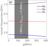
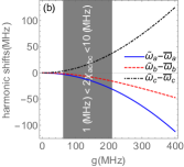
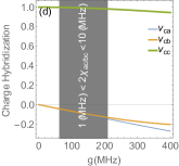
Figure 14: Normal mode quantities as a function of qubit-resonator coupling: (a) harmonic frequencies, (b) harmonic frequency shifts, (c) projection of bare qubit flux quadrature onto the normal flux quadratures, and (d) projection of the bare resonator charge quadrature that quantifies the direct drive on each normal mode. System parameters are the same as Fig. 3. Here, the resonator-qubit couplings are tuned according to $1.764g_{b}\approx g_{a}\equiv g$ such that the dispersive shifts are almost equal. The gray region provides the coupling range for which the full dispersive shift for the qubits range approximately between 1 to 10 MHz that is relevant to RIP gate implementation.

In Eqs. (76a)–(76b), $u_{kk^{\prime}}$ and $v_{kk^{\prime}}$ are matrix elements of $\mathbf{U}$ and $\mathbf{V}$ for $k,k^{\prime}=a,b,c$. Normal mode harmonic frequencies are denoted by a tilde to distinguish them from the renormalized (Lamb-shifted) normal frequencies (see Appendix F). Note that due to the inductive nature of the Josephson potential, nonlinear processes appear only via mixing of flux hybridization coefficients. On the other hand, a fraction of the RIP drive acts on the normal qubit modes through charge hybridization. Figure 14 shows the dependence of normal mode quantities on qubit-resonator couplings $g_{a,b}$.

Appendix D Displacement transformation of the resonator mode

Here, we apply a displacement transformation on the normal mode Hamiltonian (76a)–(76b) and derive an effective classical response for the resonator mode.

We adopt the following Ansatz

$$\hat{D}[d_{c}(t)]\equiv e^{d_{c}(t)\hat{c}^{{\dagger}}-d_{c}^{*}(t)\hat{c}}\;,$$ (77)

where $d_{c}(t)$ is the time-dependent coherent displacement. Here, we have used a distinct notation, compared to Eq. (30a), where $d_{c}(t)$ accounts also for possible counter-rotating contributions in the drive. The displaced-frame Hamiltonian can be written as

$$\hat{\mathcal{H}}_{s}(t)\equiv\hat{D}^{{\dagger}}[d_{c}(t)]\left[\hat{\mathcal{H}}_{s}+\hat{\mathcal{H}}_{d}(t)-i\partial_{t}\right]\hat{D}[d_{c}(t)]\;.$$ (78)

Expanding Eq. (78) in terms of $d_{c}(t)$ we find

$$\begin{split}&\hat{\mathcal{H}}_{s}(t)=\sum\limits_{k=a,b,c}\tilde{\omega}_{k}\hat{k}^{{\dagger}}\hat{k}+\tilde{\omega}_{c}[d_{c}^{*}(t)\hat{c}+\text{H.c.}]\\ &+\sum\limits_{j=a,b}\sum\limits_{n=2}^{\infty}\frac{\bar{\omega}_{j}}{2}(-\epsilon_{j})^{n-1}\frac{\left[\sum\limits_{k=a,b,c}u_{jk}\hat{k}+u_{jc}d_{c}(t)+\text{H.c.}\right]^{2n}}{(2n)!}\\ &+i[\sum\limits_{j=a,b,c}v_{cj}\hat{j}-\text{H.c.}][\Omega_{cx}(t)\cos(\omega_{d}t)+\Omega_{cy}(t)\cos(\omega_{d}t)]\\ &+i[\dot{d}_{c}^{*}(t)\hat{c}-\text{H.c.}]\;.\end{split}$$ (79)

Coherent displacement $d_{c}(t)$ is then set such that terms linear in $\hat{c}$ and $\hat{c}^{{\dagger}}$ are canceled out in the displaced Hamiltonian (79). Note that such terms can also emerge from the anharmonic part of Hamiltonian (79) due to the non-commuting bosonic algebra. Following this procedure up to the quartic expansion we find

$$\begin{split}\dot{d}_{c}(t)=&-i\tilde{\omega}_{c}d_{c}(t)-v_{cc}[\Omega_{cx}(t)\cos(\omega_{d}t)+\Omega_{cy}(t)\sin(\omega_{d}t)]\\ &-i\delta_{c}[d_{c}(t)+d_{c}^{*}(t)]\\ &-\frac{i}{3}\alpha_{c}[d_{c}(t)+d_{c}^{*}(t)]^{3}+O(\epsilon^{2})\;.\end{split}$$ (80)

The first line of Eq. (80) contains the terms coming from the harmonic Hamiltonian. The second and the third lines, however, contain nonlinear corrections, from which we find a static frequency shift as well as an effective anharmonicity for the resonator mode as

$$\begin{split}\delta_{Sc}\equiv&-\frac{1}{4}\epsilon_{a}\bar{\omega}_{a}u_{ac}^{2}\left(u_{aa}^{2}+u_{ab}^{2}+u_{ac}^{2}\right)\\ &-\frac{1}{4}\epsilon_{b}\bar{\omega}_{b}u_{bc}^{2}\left(u_{ba}^{2}+u_{bb}^{2}+u_{bc}^{2}\right)+O(\epsilon^{2})\;,\end{split}$$ (81)

$$\alpha_{c}\equiv -\frac{1}{4}\left(\epsilon_{a}\bar{\omega}_{a}u_{ac}^{4}+\epsilon_{b}\bar{\omega}_{b}u_{bc}^{4}\right)+O(\epsilon^{2})\;.$$ (82)

Equation (80) determines $d_{c}(t)$ as the response of a driven classical Duffing oscillator. Resorting to Eq. (80) is needed when the RIP drive is comparatively strong. In the rotating frame of the drive and under the RWA, a simplified equation for the slowly varying amplitude $d_{c}(t)\equiv\eta_{c}(t)e^{-i\omega_{d}t}$ is obtained as

$$\dot{\eta}_{c}(t)+i\Delta_{cd}\eta_{c}(t)+i\alpha_{c}|\eta_{c}(t)|^{2}\eta_{c}(t)=-\frac{i}{2}\Omega_{c}(t)\;,$$ (83)

where $\omega_{c}\equiv\tilde{\omega}_{c}+\delta_{Sc}$, $\Delta_{cd}\equiv\omega_{c}-\omega_{d}$ and $\Omega_{c}(t)=\Omega_{cy}(t)-i\Omega_{cx}(t)$. We note that higher order terms, e.g. coming from the sextic nonlinearity, can become relevant in the strong drive regime. For typical RIP parameters, $v_{cc}\approx 0.99$, leading to a negligible renormalization of the intended RIP drive amplitude which is neglected for simplicity.

Appendix E Resonator response and leakage

A possible source of coherent error for the RIP gate is residual resonator photon population at the end of the pulse leading to a faulty $ZZ$ interaction. Here, we analyze the resonator response based on condition (83) and discuss parameter choices that suppress leakage. We provide a classical leakage measure [Eq. (88)], which relates the relative resonator leakage to the resonator-drive detuning and pulse duration. Furthermore, we demonstrate the advantage of adding DRAG to the resonator drive in suppressing leakage.

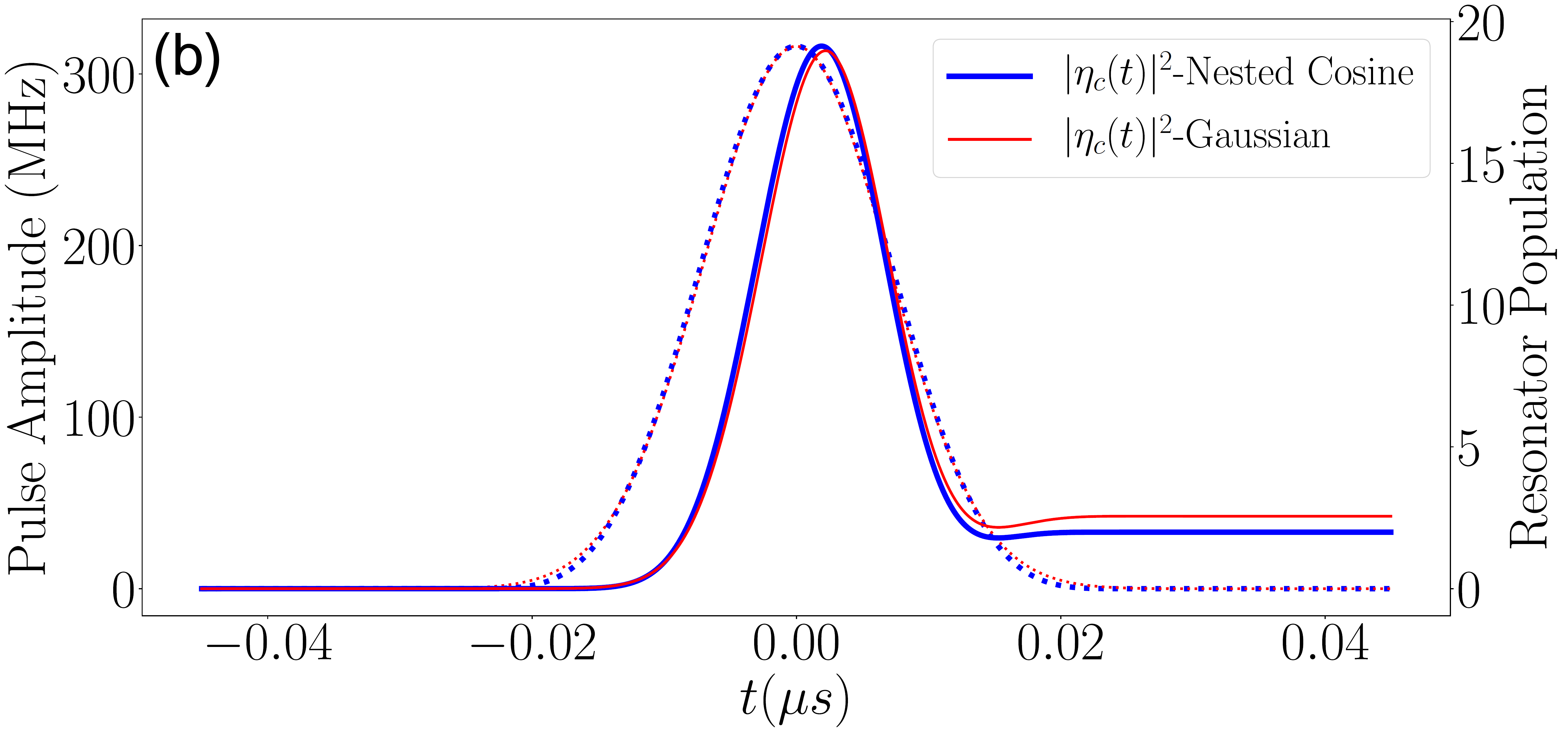
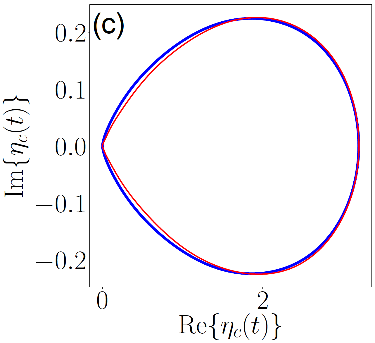
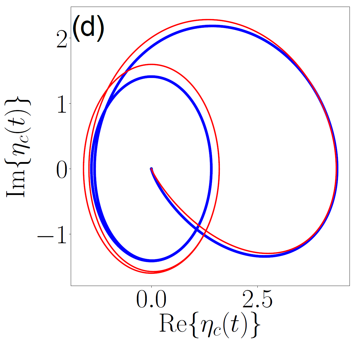
Figure 15: Dependence of residual photon population on pulse time $\mathbf{\tau}$ based on Eq. (83). Resonator and drive parameters are set as $\Delta_{cd}/2\pi=-50$ MHz, $\Omega_{c}/2\pi=316.227$ MHz and $\alpha_{c}/2\pi=0$. The pulse time is set to $\tau=200$ ns for (a) and (c) and to $\tau=50$ ns for (b) and (d). The input pulse and the resonator response are shown in dotted and solid curves, respectively. Shorter pulse time leads to larger residual photon population, which is seen as a steady-state orbit around the origin in phase space.

For comparison, we consider two pulse shapes. Firstly, a truncated Gaussian pulse as

$$\Omega_{cy}(t)=\Omega_{c}P_{G}(t;t_{\text{G}},\sigma,\tau)\;,$$ (84a)

$$P_{\text{G}}(t;t_{G},\sigma,\tau)\equiv\frac{e^{-\frac{(t-t_{G})^{2}}{2\sigma^{2}}}-e^{-\frac{\tau^{2}}{8\sigma^{2}}}}{1-e^{-\frac{\tau^{2}}{8\sigma^{2}}}}\;,$$ (84b)

for $-\tau/2<t-t_{\text{G}}<\tau/2$, where $\tau$ is the pulse time, $t_{\text{G}}$ is the center, $\sigma$ is the standard deviation and the pulse is forced to zero at the tails. The Gaussian pulse serves as a standard point of reference for which simple analytical solutions exist. In our numerical simulations, as well as earlier experiments Paik_Experimental_2016 , we use the nested cosine pulse defined as

$$\Omega_{cy}(t)\equiv\Omega_{c}P_{\text{nc}}(t;t_{\text{nc}},\tau)\;,$$ (85a)

$$P_{\text{nc}}(t;t_{\text{nc}},\tau)\equiv\frac{1}{2}\left\{\cos\left[\pi\cos\left(\pi\frac{t-t_{\text{nc}}}{\tau}\right)\right]+1\right\}\;,$$ (85b)

for $0<t-t_{\text{nc}}<\tau$. The advantage of the latter is its smoother rise and fall (zero first-order derivative), which mitigates residual photons Cross_Optimized_2015 . For a fair comparison, we set the area under the pulse to be equal as

$$\int_{t_{\text{nc}}}^{t_{\text{nc}}+\tau}dtP_{\text{nc}}(t;t_{\text{nc}},\tau)=\int_{t_{\text{G}}-\tau/2}^{t_{\text{G}}+\tau/2}dtP_{\text{G}}(t;t_{\text{G}},\sigma,\tau)\;,$$ (86)

resulting in $\tau\approx 7.182\sigma$. Furthermore, to align the pulse centers, we set $t_{\text{nc}}+\tau/2=t_{\text{G}}$.

The solution to Eq. (83) depends on four independent parameters: resonator-drive detuning $\Delta_{cd}$, pulse amplitude $\Omega_{c}$, pulse time $\tau$ and resonator anharmonicity $\alpha_{c}$. In the following, we discuss two separate interplays between these parameters. Firstly, the ratio of residual photons to the intended maximum photon number depends primarily on the product $\Delta_{cd}\tau$. To focus on this, we first set $\alpha_{c}$ to zero. Figure 15 compares the resonator response for two pulse times of $\tau=200$ ns and $\tau=50$ ns and fixed $\Delta_{cd}/2\pi=-50$ MHz. We observe a significantly larger residual photon population for $\tau=50$ ns for both pulse forms, but the nested cosine pulse results in a smaller population than the Gaussian pulse. The increase in residual photons for the shorter pulse duration can be understood as the pulse becoming broader in the frequency domain leading to a larger overlap with the resonator and hence a transfer of energy to the resonator mode.

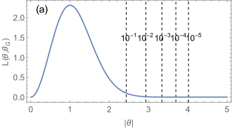
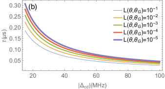
Figure 16: (a) Normalized leakage function $L(\theta,\theta_{\text{G}})$ in Eq. (88). Vertical dashed lines show values of $\theta\equiv\Delta_{cd}\sigma$ that $L(\theta,\theta_{G})$ is fixed to in panel (b). (b) Corresponding constant leakage contours as a function of $\tau$ and $\Delta_{cd}$ using the relation $\tau\approx 7.182\sigma$.

In the linear case, i.e. $\alpha_{c}/2\pi=0$, it is possible to obtain an analytical solution to Eq. (83). For clarity, consider a non-truncated Gaussian input as $\Omega_{c}(t)=\Omega_{c}\exp[(t-t_{\text{G}})^{2}/2\sigma^{2}]$. The solution with initial zero resonator photons [i.e. $\eta_{c}(0)=0$] reads

$$\begin{split}&\eta_{c}(t)=-\frac{i}{2}\Omega_{c}\sqrt{\frac{\pi}{2}}\sigma e^{-\frac{1}{2}\Delta_{cd}^{2}\sigma^{2}}e^{-i\Delta_{cd}(t-t_{\text{G}})}\\ &\times\left[\text{erf}\left(\frac{t-t_{\text{G}}}{\sqrt{2}\sigma}-i\frac{\Delta_{cd}\sigma}{\sqrt{2}}\right)+\text{erf}\left(\frac{t_{G}}{\sqrt{2}\sigma}+i\frac{\Delta_{cd}\sigma}{\sqrt{2}}\right)\right]\;,\end{split}$$ (87)

where $\text{erf}(x)\equiv(2/\sqrt{\pi})\int_{0}^{x}dz\exp(-z^{2})$ is the error function. The residual photon population can be defined, based on solution (87), as the steady-state response $n_{c}(\infty)\equiv\lim\limits_{t\to\infty}|\eta_{c}(t)|^{2}$. We then define a normalized leakage measure as the ratio of residual photon population to the intended maximum photon population as

$$L(\theta,\theta_{\text{G}})\equiv\frac{n_{c}(\infty)}{(\frac{\Omega_{c}}{2\Delta_{cd}})^{2}}=\frac{\pi}{2}\theta^{2}e^{-\theta^{2}}\left|1+\text{erf}\left(\frac{i\theta^{2}+\theta_{\text{G}}}{\sqrt{2}\theta}\right)\right|^{2}\;,$$ (88)

where $\theta\equiv\Delta_{cd}\sigma$ and $\theta_{\text{G}}\equiv\Delta_{cd}t_{\text{G}}$ are unitless angles denoting the width and center of the pulse, respectively, with the assumption $\theta_{G}\gg\theta>0$. According to Eq. (88), for $\theta\ll 1$, the leakage grows as $\theta^{2}$, while an exponential suppression of the form $\exp(-\theta^{2})$ is expected for $\theta\gg 1$ [see Fig. 16].

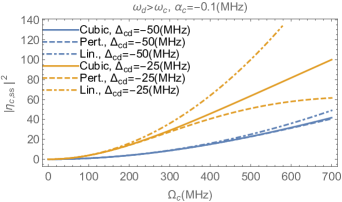
Figure 17: Steady-state resonator photon number as a function of RIP drive for $\Delta_{cd}/2\pi=-50$ MHz (blue) and $\Delta_{cd}/2\pi=-25$ MHz (yellow). Resonator anharmonicity is set to $\alpha_{c}/2\pi=-100$ KHz. Solid lines are found via exact solution to Eq. (90), dashed lines show the first order expansion in $|\alpha_{c}/\Delta_{cd}|$ based on Eq. (91) and the dashed-dotted lines show the commonly used linear estimate $|\Omega_{c}/(2\Delta_{cd})|^{2}$. We find that for smaller resonator-drive detuning and stronger drive, it becomes more important to account for the resonator anharmonicity.

Secondly, based on Eq. (83) and up to lowest order in $|\alpha_{c}/\Delta_{cd}|$, the effect of resonator anharmonicity on leakage is a dynamic shift of the resonator-drive detuning as

$$\Delta_{cd}(t)\equiv\Delta_{cd}+\alpha_{c}|\eta_{c}(t)|^{2}\;.$$ (89)

Following the linear leakage measure (88), if the anharmonicity increases (decreases) the effective $\Delta_{cd}(t)$, it leads to suppression (enhancement) of resonator leakage. Since $\alpha_{c}$ is intrinsically negative (softening Josephson nonlinearity), having $\Delta_{cd}<0$ (drive above resonator frequency) is beneficial. This heuristic argument is confirmed by numerical solution to Eq. (83), where we find this effect to become relevant at stronger photon number of the order $|\eta_{c}(t)|^{2}\sim|\Delta_{cd}/\alpha_{c}|$. A typical RIP design leads to $50\ \text{KHz}<|\alpha_{c}/2\pi|<100\ \text{KHz}$.

Furthermore, for strong RIP drive, the resonator anharmonicity must be accounted for in our estimate for the maximum photon number. Based on Eq. (83), the steady-state response satisfies

$$\Delta_{cd}\eta_{c,\text{ss}}+\alpha_{c}|\eta_{c,\text{ss}}|^{2}\eta_{c,\text{ss}}=-\frac{1}{2}\Omega_{c}\;,$$ (90)

whose approximate solution can be obtained as

$$\eta_{c,\text{ss}}=-\frac{\Omega_{c}}{2\left[\Delta_{cd}+\alpha_{c}\left(\frac{\Omega_{c}}{2\Delta_{cd}}\right)^{2}\right]}+O(|\frac{\alpha_{c}}{\Delta_{cd}}|^{2})\;.$$ (91)

Figure 17 makes a comparison between the different estimates for steady-state resonator photon number.

Operator	Coefficient	Normal-mode expression	Estimate (MHz)
$\hat{a}$	$\lambda_{a}(t)$	$\frac{v_{ca}\Omega_{c}(t)}{2}-\frac{\epsilon_{a}\bar{\omega}_{a}}{4}u_{aa}u_{ac}\left[u_{aa}^{2}+u_{ab}^{2}+u_{ac}^{2}\left(1+|\eta_{c}(t)|^{2}\right)\right]\eta_{c}^{*}(t)$ $-\frac{\epsilon_{b}\bar{\omega}_{b}}{4}u_{ba}u_{bc}\left[u_{ba}^{2}+u_{bb}^{2}+u_{bc}^{2}\left(1+|\eta_{c}(t)|^{2}\right)\right]\eta_{c}^{*}(t)$	$-0.052\Omega_{c}(t)-26.466\eta_{c}^{*}(t)$ $-0.282|\eta_{c}(t)|^{2}\eta_{c}^{*}(t)$
$\hat{b}$	$\lambda_{b}(t)$	$\frac{v_{cb}\Omega_{c}(t)}{2}-\frac{\epsilon_{a}\bar{\omega}_{a}}{4}u_{ab}u_{ac}\left[u_{aa}^{2}+u_{ab}^{2}+u_{ac}^{2}\left(1+|\eta_{c}(t)|^{2}\right)\right]\eta_{c}^{*}(t)$ $-\frac{\epsilon_{b}\bar{\omega}_{b}}{4}u_{bb}u_{bc}\left[u_{ba}^{2}+u_{bb}^{2}+u_{bc}^{2}\left(1+|\eta_{c}(t)|^{2}\right)\right]\eta_{c}^{*}(t)$	$-0.049\Omega_{c}(t)-26.654\eta_{c}^{*}(t)$ $-0.264|\eta_{c}(t)|^{2}\eta_{c}^{*}(t)$
$\hat{a}^{{\dagger}}\hat{a}$	$\delta_{Sa}$	$-\frac{1}{4}\epsilon_{a}\bar{\omega}_{a}u_{aa}^{2}\left(u_{aa}^{2}+u_{ab}^{2}+u_{ac}^{2}\right)-\frac{1}{4}\epsilon_{b}\bar{\omega}_{b}u_{ba}^{2}\left(u_{ba}^{2}+u_{bb}^{2}+u_{bc}^{2}\right)$	$-252.004$
$\hat{b}^{{\dagger}}\hat{b}$	$\delta_{Sb}$	$-\frac{1}{4}\epsilon_{a}\bar{\omega}_{a}u_{ab}^{2}\left(u_{aa}^{2}+u_{ab}^{2}+u_{ac}^{2}\right)-\frac{1}{4}\epsilon_{b}\bar{\omega}_{b}u_{bb}^{2}\left(u_{ba}^{2}+u_{bb}^{2}+u_{bc}^{2}\right)$	$-272.309$
$\hat{c}^{{\dagger}}\hat{c}$	$\delta_{Sc}$	$-\frac{1}{4}\epsilon_{a}\bar{\omega}_{a}u_{ac}^{2}\left(u_{aa}^{2}+u_{ab}^{2}+u_{ac}^{2}\right)-\frac{1}{4}\epsilon_{b}\bar{\omega}_{b}u_{bc}^{2}\left(u_{ba}^{2}+u_{bb}^{2}+u_{bc}^{2}\right)$	$-5.439$
$\hat{a}^{{\dagger}}\hat{a}$	$\delta_{Da}(t)$	$-\frac{1}{2}\left(\epsilon_{a}\bar{\omega}_{a}u_{aa}^{2}u_{ac}^{2}+\epsilon_{b}\bar{\omega}_{b}u_{ba}^{2}u_{bc}^{2}\right)|\eta_{c}(t)|^{2}$	$-5.371|\eta_{c}(t)|^{2}$
$\hat{b}^{{\dagger}}\hat{b}$	$\delta_{Db}(t)$	$-\frac{1}{2}\left(\epsilon_{a}\bar{\omega}_{a}u_{ab}^{2}u_{ac}^{2}+\epsilon_{b}\bar{\omega}_{b}u_{bb}^{2}u_{bc}^{2}\right)|\eta_{c}(t)|^{2}$	$-5.395|\eta_{c}(t)|^{2}$
$\hat{c}^{{\dagger}}\hat{c}$	$\delta_{Dc}(t)$	$-\frac{1}{2}\left(\epsilon_{a}\bar{\omega}_{a}u_{ac}^{4}+\epsilon_{b}\bar{\omega}_{b}u_{bc}^{4}\right)|\eta_{c}(t)|^{2}$	$-0.112|\eta_{c}(t)|^{2}$
$\hat{a}^{{\dagger}}\hat{b}$	$\lambda_{a^{*}b}(t)$	$-\frac{\epsilon_{a}\bar{\omega}_{a}}{4}u_{aa}u_{ab}\left[u_{aa}^{2}+u_{ab}^{2}+u_{ac}^{2}\left(1+2|\eta_{c}(t)|^{2}\right)\right]$ $-\frac{\epsilon_{b}\bar{\omega}_{b}}{4}u_{ba}u_{bb}\left[u_{ba}^{2}+u_{bb}^{2}+u_{bc}^{2}\left(1+2|\eta_{c}(t)|^{2}\right)\right]$	$2.436+0.057|\eta_{c}(t)|^{2}$
$\hat{a}^{{\dagger}}\hat{c}$	$\lambda_{a^{*}c}(t)$	$-\frac{\epsilon_{a}\bar{\omega}_{a}}{4}u_{aa}u_{ac}\left[u_{aa}^{2}+u_{ab}^{2}+u_{ac}^{2}\left(1+2|\eta_{c}(t)|^{2}\right)\right]$ $-\frac{\epsilon_{b}\bar{\omega}_{b}}{4}u_{ba}u_{bc}\left[u_{ba}^{2}+u_{bb}^{2}+u_{bc}^{2}\left(1+2|\eta_{c}(t)|^{2}\right)\right]$	$-26.466-0.563|\eta_{c}(t)|^{2}$
$\hat{b}^{{\dagger}}\hat{c}$	$\lambda_{b^{*}c}(t)$	$-\frac{\epsilon_{a}\bar{\omega}_{a}}{4}u_{ab}u_{ac}\left[u_{aa}^{2}+u_{ab}^{2}+u_{ac}^{2}\left(1+2|\eta_{c}(t)|^{2}\right)\right]$ $-\frac{\epsilon_{b}\bar{\omega}_{b}}{4}u_{bb}u_{bc}\left[u_{ba}^{2}+u_{bb}^{2}+u_{bc}^{2}\left(1+2|\eta_{c}(t)|^{2}\right)\right]$	$-26.654-0.527|\eta_{c}(t)|^{2}$
$\hat{a}^{{\dagger}}\hat{a}\hat{a}$	$\lambda_{a^{*}aa}(t)$	$-\frac{1}{4}(\epsilon_{a}\bar{\omega}_{a}u_{aa}^{3}u_{ac}+\epsilon_{b}\bar{\omega}_{b}u_{ba}^{3}u_{bc})\eta_{c}^{*}(t)$	$-25.867\eta_{c}^{*}(t)$
$\hat{b}^{{\dagger}}\hat{b}\hat{b}$	$\lambda_{b^{*}bb}(t)$	$-\frac{1}{4}(\epsilon_{a}\bar{\omega}_{a}u_{ab}^{3}u_{ac}+\epsilon_{b}\bar{\omega}_{b}u_{bb}^{3}u_{bc})\eta_{c}^{*}(t)$	$-26.954\eta_{c}^{*}(t)$
$\hat{c}^{{\dagger}}\hat{c}\hat{c}$	$\lambda_{c^{*}cc}(t)$	$-\frac{1}{4}(\epsilon_{a}\bar{\omega}_{a}u_{ac}^{4}+\epsilon_{b}\bar{\omega}_{b}u_{bc}^{4})\eta_{c}^{*}(t)$	$-0.056\eta_{c}^{*}(t)$
$\hat{a}^{{\dagger}}\hat{a}\hat{b}$	$\lambda_{a^{*}ab}(t)$	$-\frac{1}{2}(\epsilon_{a}\bar{\omega}_{a}u_{aa}^{2}u_{ab}u_{ac}+\epsilon_{b}\bar{\omega}_{b}u_{ba}^{2}u_{bb}u_{bc})\eta_{c}^{*}(t)$	$1.127\eta_{c}^{*}(t)$
$\hat{a}^{{\dagger}}\hat{a}\hat{c}$	$\lambda_{a^{*}ac}(t)$	$-\frac{1}{2}(\epsilon_{a}\bar{\omega}_{a}u_{aa}^{2}u_{ac}^{2}+\epsilon_{b}\bar{\omega}_{b}u_{ba}^{2}u_{bc}^{2})\eta_{c}^{*}(t)$	$-5.371\eta_{c}^{*}(t)$
$\hat{b}^{{\dagger}}\hat{b}\hat{a}$	$\lambda_{b^{*}ba}(t)$	$-\frac{1}{2}(\epsilon_{a}\bar{\omega}_{a}u_{ab}^{2}u_{aa}u_{ac}+\epsilon_{b}\bar{\omega}_{b}u_{bb}^{2}u_{ba}u_{bc})\eta_{c}^{*}(t)$	$-0.636\eta_{c}^{*}(t)$
$\hat{b}^{{\dagger}}\hat{b}\hat{c}$	$\lambda_{b^{*}bc}(t)$	$-\frac{1}{2}(\epsilon_{a}\bar{\omega}_{a}u_{ab}^{2}u_{ac}^{2}+\epsilon_{b}\bar{\omega}_{b}u_{bb}^{2}u_{bc}^{2})\eta_{c}^{*}(t)$	$-5.395\eta_{c}^{*}(t)$
$\hat{c}^{{\dagger}}\hat{c}\hat{a}$	$\lambda_{c^{*}ca}(t)$	$-\frac{1}{2}(\epsilon_{a}\bar{\omega}_{a}u_{ac}^{3}u_{aa}+\epsilon_{b}\bar{\omega}_{b}u_{bc}^{3}u_{ba})\eta_{c}^{*}(t)$	$-0.564\eta_{c}^{*}(t)$
$\hat{c}^{{\dagger}}\hat{c}\hat{b}$	$\lambda_{c^{*}cb}(t)$	$-\frac{1}{2}(\epsilon_{a}\bar{\omega}_{a}u_{ac}^{3}u_{ab}+\epsilon_{b}\bar{\omega}_{b}u_{bc}^{3}u_{bb})\eta_{c}^{*}(t)$	$-0.527\eta_{c}^{*}(t)$
$\frac{1}{2}\hat{a}^{{\dagger}}\hat{a}^{{\dagger}}\hat{a}\hat{a}$	$\alpha_{a}$	$-\frac{1}{4}\left(\epsilon_{a}\bar{\omega}_{a}u_{aa}^{4}+\epsilon_{b}\bar{\omega}_{b}u_{ba}^{4}\right)$	$-249.164$
$\frac{1}{2}\hat{b}^{{\dagger}}\hat{b}^{{\dagger}}\hat{b}\hat{b}$	$\alpha_{b}$	$-\frac{1}{4}\left(\epsilon_{a}\bar{\omega}_{a}u_{ab}^{4}+\epsilon_{b}\bar{\omega}_{b}u_{bb}^{4}\right)$	$-269.458$
$\frac{1}{2}\hat{c}^{{\dagger}}\hat{c}^{{\dagger}}\hat{c}\hat{c}$	$\alpha_{c}$	$-\frac{1}{4}\left(\epsilon_{a}\bar{\omega}_{a}u_{ac}^{4}+\epsilon_{b}\bar{\omega}_{b}u_{bc}^{4}\right)$	$-0.056$
$\hat{a}^{{\dagger}}\hat{a}\hat{b}^{{\dagger}}\hat{b}$	$2\chi_{ab}$	$-\frac{1}{2}\left(\epsilon_{a}\bar{\omega}_{a}u_{aa}^{2}u_{ab}^{2}+\epsilon_{b}\bar{\omega}_{b}u_{ba}^{2}u_{bb}^{2}\right)$	$-0.309$
$\hat{a}^{{\dagger}}\hat{a}\hat{c}^{{\dagger}}\hat{c}$	$2\chi_{ac}$	$-\frac{1}{2}\left(\epsilon_{a}\bar{\omega}_{a}u_{aa}^{2}u_{ac}^{2}+\epsilon_{b}\bar{\omega}_{b}u_{ba}^{2}u_{bc}^{2}\right)$	$-5.371$
$\hat{b}^{{\dagger}}\hat{b}\hat{c}^{{\dagger}}\hat{c}$	$2\chi_{bc}$	$-\frac{1}{2}\left(\epsilon_{a}\bar{\omega}_{a}u_{ab}^{2}u_{ac}^{2}+\epsilon_{b}\bar{\omega}_{b}u_{bb}^{2}u_{bc}^{2}\right)$	$-5.395$

Table 3: Dominant multimode interaction contributions (causing at most single-excitation transitions) via normal ordering of the quartic nonlinearity in Eq. (79). For brevity, the Hermitian conjugates of the unbalanced operators are not shown. From top to bottom, the contributions include direct drive on qubits coming from both linear charge and nonlinear flux hybridization, static and dynamic frequency shifts, exchange interactions, self and cross number-quadrature interactions, and self-Kerr (anharmonicity) and cross-Kerr interactions. Terms equivalent to $\hat{\sigma}_{a,b}^{z}\hat{c}+\text{H.c.}$ of the dispersive JC model, mainly responsible for the effective RIP interaction, are highlighted in boldface. Importantly, we find $\lambda_{a^{*}ac}=2\chi_{ac}\eta_{c}^{*}(t)$, $\lambda_{b^{*}bc}=2\chi_{bc}\eta_{c}^{*}(t)$, which is consistent with adopting phenomenological models from the outset. For simplicity, the estimates are given after doing the RWA on the displacement. For instance, terms that are proportional to $|\eta_{c}(t)|^{2}\eta_{c}^{*}(t)$ come from $[\eta_{c}(t)e^{-i\omega_{d}t}+\eta_{c}^{*}(t)e^{+i\omega_{d}t}]^{3}$. Circuit parameters are the same as Fig 14. According to Eqs. (75a)–(75b), the flux and charge hybridization coefficients are found as $\mathbf{U}=\big{(}\begin{smallmatrix}0.994229&-0.0217913&0.103214\\ 0.0112824&0.994923&0.0995246\\ -0.0805908&-0.0853793&0.992933\\ \end{smallmatrix}\big{)}$ and $\mathbf{V}=\big{(}\begin{smallmatrix}0.997153&-0.0192382&0.0792791\\ 0.0128348&0.996284&0.0867091\\ -0.104939&-0.0978607&0.990185\\ \end{smallmatrix}\big{)}$. Furthermore, based on Eq. (74), the normal mode frequencies are found as $\tilde{\omega}_{a}/2\pi\approx 5375.850$ MHz, $\tilde{\omega}_{b}/2\pi\approx 6107.200$ MHz and $\tilde{\omega}_{c}/2\pi\approx 7019.430$ MHz.

Lastly, we discuss the benefit of DRAG Motzoi_Simple_2009 ; Gambetta_Analytic_2011 ; Malekakhlagh_Mitigating_2021 in mitigating the resonator leakage. Consider a complex-valued control pulse as $\Omega_{c}(t)=\Omega_{cy}-i\Omega_{cx}(t)$, and, for simplicity, assume that the contribution due to $\alpha_{c}$ in Eq. (83) is negligible. In the frequency domain, the solution reads $\tilde{\eta}_{c}(\omega)=-\tilde{\Omega}_{c}(\omega)/[2(\omega+\Delta_{cd})]$. To mitigate leakage, the pulse should have minimal frequency content at $\omega=-\Delta_{cd}$. Consider an Ansatz for a DRAG pulse as

$$\Omega_{cy}(t)=\Omega_{c}P_{\text{nc}}(t;0,\tau)\;,$$ (92a)

$$\Omega_{cx}(t)=\frac{1}{\Delta_{D}}\Omega_{c}\dot{P}_{\text{nc}}(t;0,\tau)\;,$$ (92b)

with $\Delta_{D}$ as the DRAG parameter. Given that $\partial_{t}\leftrightarrow i\omega$, the corresponding transfer function for DRAG is $\tilde{\Omega}_{c}(\omega)=\Omega_{c}T_{D}(\omega)\tilde{P}_{\text{nc}}(\omega)$ where $T_{D}(\omega)=1+\omega/\Delta_{D}$. Therefore, DRAG acts as an effective notch filter and setting $\Delta_{D}=\Delta_{cd}$ results in a zero in the pulse spectrum. In Fig. 5, using the exact ab-initio simulation, it is shown that such a DRAG pulse can improve the background resonator leakage by at least one order of magnitude at small $\Delta_{cd}$.

In summary, we have characterized the resonator response in terms of a driven classical Kerr oscillator. Comparing two pulse shapes, Gaussian and nested cosine, we confirmed that the nested cosine pulse results in slightly improved resonator leakage due to smoother rise and fall. We introduced a classical leakage measure in Eq. (88) and Fig. 16, which characterizes the trade-off between pulse time and resonator-drive detuning. Furthremore, employing a DRAG pulse proves to be very helpful in suppressing background leakage (see Sec. IV and Fig. 5).

Appendix F Approximate ab-initio model

In this appendix, starting from the displaced Hamiltonian (79), we construct an approximate ab-initio model Hamiltonian. There are numerous processes that originate from the Taylor expansion of the cosine nonlinearity. Here, up to the quartic expansion, we read off dominant interaction terms by first performing normal ordering of the nonlinearity using SNEG Zitko_Sneg_2011 and then regrouping the terms into zeroth order and interaction parts. The advantage of normal ordering is that it leads to a lower number of interaction forms while applying SWPT (discussed in Appendix G).

We group the terms in Eq. (79) as

$$\hat{\mathcal{H}}_{s}(t)=\hat{\mathcal{H}}_{0}+\hat{\mathcal{H}}_{\text{int}}(t)\;,$$ (93)

where $\hat{\mathcal{H}}_{0}$ contains time-independent diagonal contributions and up to the quartic expansion is the same as the Kerr model:

$$\begin{split}\hat{\mathcal{H}}_{0}&=\sum\limits_{j=a,b,c}\left[\omega_{j}\hat{n}_{j}+\frac{\alpha_{j}}{2}\hat{n}_{j}(\hat{n}_{j}-1)\right]\\ &+\sum\limits_{j,k=a,b,c\atop j>k}2\chi_{jk}\hat{n}_{j}\hat{n}_{k}\;.\end{split}$$ (94)

In Eq. (94), $\omega_{j}\equiv\tilde{\omega}_{j}+\delta_{Sj}$ is the renormalized frequency for mode $j=a,b,c$ accounting for the static frequency shift. Effective anharmonicity of the normal modes and the pairwise cross-Kerr interactions are denoted by $\alpha_{j}$ and $2\chi_{jk}$ for $j,k=a,b,c$ (see Table 3 for the definitions). Moreover, $\hat{\mathcal{H}}_{\text{int}}(t)$ is the perturbation consisting of the rest of the time-dependent nonlinear contributions of the generic form

$$(\hat{a}^{{\dagger}})^{i}\hat{a}^{j}(\hat{b}^{{\dagger}})^{k}\hat{b}^{l}(\hat{c}^{{\dagger}})^{m}\hat{c}^{n}[\eta^{*}(t)]^{p}[\eta_{c}(t)]^{q}e^{i(p-q)\omega_{d}t}\;,$$ (95)

where the sum of exponents should match the order of expansion in the cosine nonlinearity. For our approximate model, we keep contributions that are either balanced (equal number of creation and annihilation) or have a comparably small energy difference (single-excitation) as

$$\begin{split}\hat{\mathcal{H}}_{\text{int}}(t)&=\sum\limits_{j=a,b,c}\delta_{Dj}(t)\hat{n}_{j}\\ &+\sum\limits_{j=a,b}[\lambda_{j}(t)e^{i\omega_{d}t}\hat{j}+\text{H.c.}]\\ &+\sum\limits_{j,k=a,b,c\atop j>k}[\lambda_{j^{*}k}(t)\hat{j}^{{\dagger}}\hat{k}+\text{H.c.}]\\ &+\sum\limits_{j,k=a,b,c}[\lambda_{j^{*}jk}(t)e^{i\omega_{d}t}\hat{n}_{j}\hat{k}+\text{H.c.}]\;.\\ \end{split}$$ (96)

Table 3 summarizes such interaction terms and provides an estimate based on quartic expansion of Eq. (79).

In summary, compared to the phenomenological Kerr model of Appendix B, we accounted for a few additional interaction forms. Namely, the second line of Eq. (96) is an unwanted drive term acting on the qubit modes. The third line contains exchange interactions between the normal modes. Finally, the last line contains all possible number-quadrature interactions. In Appendix G, we find that the dominant source of RIP interaction is an interplay between the interaction forms $\lambda_{a^{*}ac}(t)\hat{a}^{{\dagger}}\hat{a}\hat{c}+\text{H.c.}$ and $\lambda_{b^{*}bc}(t)\hat{b}^{{\dagger}}\hat{b}\hat{c}+\text{H.c.}$ . Moreover, from normal ordering of the nonlinearity, we obtain $\lambda_{a^{*}ac}(t)=2\chi_{ac}\hat{\eta}_{c}^{*}(t)$ and $\lambda_{b^{*}bc}(t)=2\chi_{bc}\hat{\eta}_{c}^{*}(t)$ in agreement with the phenomenological Kerr model (see Table 3).

Appendix G Effective Hamiltonian based on the approximate ab-initio model

Here, using time-dependent SWPT, we derive an effective RIP Hamiltonian based on the ab-initio model in Eqs. (94) and (96). Compared to the phenomenological Kerr model in Appendix B, we find corrections to both the intended RIP interaction as well as a series of new effective interaction forms.

To simplify perturbation, we first obtain the interaction-frame Hamiltonian based on Eqs. (94) and (96). Employing identities (46d)–(46e), the annihilation operator for each mode transforms as

$$e^{i\hat{\mathcal{H}}_{0}t}\hat{j}e^{-i\hat{\mathcal{H}}_{0}t}=e^{-i\hat{\omega}_{j}t}\hat{j},\quad j=a,b,c\;,$$ (97a)

where we have defined operator-valued normal mode frequencies as

$$\hat{\omega}_{a}\equiv\omega_{a}+\alpha_{a}\hat{n}_{a}+2\chi_{ab}\hat{n}_{b}+2\chi_{ac}\hat{n}_{c}\;,$$ (97b)

$$\hat{\omega}_{b}\equiv\omega_{b}+2\chi_{ab}\hat{n}_{a}+\alpha_{b}\hat{n}_{b}+2\chi_{bc}\hat{n}_{c}\;,$$ (97c)

$$\hat{\omega}_{c}\equiv\omega_{c}+2\chi_{ac}\hat{n}_{a}+2\chi_{bc}\hat{n}_{b}+\alpha_{c}\hat{n}_{c}\;.$$ (97d)

Using Eqs. (97a)–(97d), we find the interaction-frame Hamiltonian as

$$\begin{split}\hat{\mathcal{H}}_{I}(t)&\equiv e^{i\hat{\mathcal{H}}_{0}t}\hat{\mathcal{H}}_{\text{int}}(t)e^{-i\hat{\mathcal{H}}_{0}t}\\ &=\sum\limits_{j=a,b,c}\delta_{Dj}(t)\hat{n}_{j}\\ &+\sum\limits_{j=a,b}[\lambda_{j}(t)e^{-i\hat{\Delta}_{jd}t}\hat{j}+\text{H.c.}]\\ &+\sum\limits_{j,k=a,b,c\atop j>k}[\lambda_{j^{*}k}(t)\hat{j}^{{\dagger}}e^{i\hat{\Delta}_{jk}t}\hat{k}+\text{H.c.}]\\ &+\sum\limits_{j,k=a,b,c}[\lambda_{j^{*}jk}(t)e^{-i\hat{\Delta}_{kd}t}\hat{n}_{j}\hat{k}+\text{H.c.}]\;,\end{split}$$ (98)

with operator-valued detunings defined as $\hat{\Delta}_{jd}\equiv\hat{\omega}_{j}-\omega_{d}$ and $\hat{\Delta}_{jk}\equiv\hat{\omega}_{j}-\hat{\omega}_{k}$ for $j,k=a,b,c$.

Up to the first order, the effective Hamiltonian contains dynamic frequency shifts, the only diagonal contribution in Eq. (98), as

$$\hat{\mathcal{H}}_{I,\text{eff}}^{(1)}(t)=\sum\limits_{j=a,b,c}\delta_{Dj}(t)\hat{n}_{j}\;.$$ (99)

The SWPT generator $\hat{G}_{1}(t)$ is then the time-integral of the rest of off-diagonal terms as

$$\begin{split}\hat{G}_{1}(t)&=\sum\limits_{j=a,b}\int^{t}dt^{\prime}[\lambda_{j}(t^{\prime})e^{-i\hat{\Delta}_{jd}t^{\prime}}\hat{j}+\text{H.c.}]\\ &+\sum\limits_{j,k=a,b,c\atop j>k}\int^{t}dt^{\prime}[\lambda_{jk}(t^{\prime})\hat{j}^{{\dagger}}e^{i\hat{\Delta}_{jk}t^{\prime}}\hat{k}+\text{H.c.}]\\ &+\sum\limits_{j,k=a,b,c}\int^{t}dt^{\prime}[\lambda_{j^{*}jk}(t^{\prime})e^{-i\hat{\Delta}_{kd}t^{\prime}}\hat{n}_{j}\hat{k}+\text{H.c.}]\;.\end{split}$$ (100)

Replacing Eq. (100) into the second order effective Hamiltonian (39a), we find that the off-diagonal terms in $\hat{G}_{1}(t)$ can generate a variety of effective diagonal interactions of the form

$$\begin{split}&\hat{\mathcal{H}}_{I,\text{eff}}^{(2)}(t)=\sum\limits_{j=a,b,c}\hat{\delta}_{j}^{(2)}(t)\hat{n}_{j}+\sum\limits_{j=a,b,c}\frac{1}{2}\hat{\alpha}_{j}^{(2)}(t)\hat{n}_{j}^{2}\\ &+\sum\limits_{j=a,b,c}\hat{\beta}_{j}^{(2)}(t)\hat{n}_{j}^{3}+\sum\limits_{j,k=a,b,c\atop j>k}2\hat{\chi}_{jk}^{(2)}(t)\hat{n}_{j}\hat{n}_{k}\\ &+\sum\limits_{j,k=a,b,c\atop j>k}\hat{\chi}_{jjk}^{(2)}(t)\hat{n}_{j}^{2}\hat{n}_{k}+\chi_{abc}^{(2)}(t)\hat{n}_{a}\hat{n}_{b}\hat{n}_{c}\;.\end{split}$$ (101)

The contributions in Eq. (101) can be summarized as second order dynamic frequency shifts, dynamic anharmonic shifts, RIP-like (number-number) interactions, higher order two-body interaction (number-squared-number) and three-body number interactions, respectively. Note that the normal resonator mode $\hat{c}$ denotes excitations on top of the coherent displacement $\eta_{c}(t)$, hence corrections involving $\hat{c}$ are expected to be orders of magnitude smaller than the ones dependent on $\eta_{c}(t)$.

In the following, we first provide the derivation for the intended RIP interaction, i.e. $\hat{\chi}_{ab}^{(2)}(t)$ and then quote the final result for the rest of the effective interaction rates. There are multiple processes that contribute to an effective $\chi_{ab}^{(2)}(t)$. From the dispersive JC model, we learned that the interplay between $\hat{\sigma}_{a}^{z}\hat{c}+\text{H.c.}$ and $\hat{\sigma}_{b}^{z}\hat{c}+\text{H.c.}$ is the dominant source. Multilevel equivalent terms are $\hat{a}^{{\dagger}}\hat{a}\hat{c}+\text{H.c.}$ and $\hat{b}^{{\dagger}}\hat{b}\hat{c}+\text{H.c.}$, highlighted in boldface in Table 3. In addition, up to the 2nd order in SWPT, we find five more possibilities for mixing: (i) $\bm{\hat{a}^{{\dagger}}\hat{a}\hat{c}+\textbf{H.c.}}$ and $\bm{\hat{b}^{{\dagger}}\hat{b}\hat{c}+\textbf{H.c.}}$, (ii) $\hat{a}^{{\dagger}}\hat{a}\hat{a}+\text{H.c.}$ and $\hat{b}^{{\dagger}}\hat{b}\hat{a}+\text{H.c.}$, (iii) $\hat{b}^{{\dagger}}\hat{b}\hat{b}+\text{H.c.}$ and $\hat{a}^{{\dagger}}\hat{a}\hat{b}+\text{H.c.}$, (iv) $\hat{a}^{{\dagger}}\hat{b}+\text{H.c.}$ and $\hat{a}^{{\dagger}}\hat{b}+\text{H.c.}$, (v) $\hat{a}+\text{H.c.}$ and $\hat{b}^{{\dagger}}\hat{b}\hat{a}+\text{H.c.}$, (vi) $\hat{b}+\text{H.c.}$ and $\hat{a}^{{\dagger}}\hat{a}\hat{b}+\text{H.c.}$.

We next analyze case (i) in more detail. The non-zero contributions coming from the interplay of $\hat{a}^{{\dagger}}\hat{a}\hat{c}+\text{H.c.}$ and $\hat{b}^{{\dagger}}\hat{b}\hat{c}+\text{H.c.}$ is found from Eq. (39a) as

$$\begin{split}\frac{i}{2}\left[\int^{t}dt^{\prime}\lambda_{a^{*}ac}(t^{\prime})e^{-i\hat{\Delta}_{cd}t^{\prime}}\hat{n}_{a}\hat{c},\lambda_{b^{*}bc}^{*}(t)\hat{n}_{b}\hat{c}^{{\dagger}}e^{i\hat{\Delta}_{cd}t}\right]+\frac{i}{2}\left[\int^{t}dt^{\prime}\lambda^{*}_{a^{*}ac}(t^{\prime})\hat{n}_{a}\hat{c}^{{\dagger}}e^{i\hat{\Delta}_{cd}t^{\prime}},\lambda_{b^{*}bc}(t)e^{-i\hat{\Delta}_{cd}t}\hat{n}_{b}\hat{c}\right]\\ +\frac{i}{2}\left[\int^{t}dt^{\prime}\lambda_{b^{*}bc}(t^{\prime})e^{-i\hat{\Delta}_{cd}t^{\prime}}\hat{n}_{b}\hat{c},\lambda_{a^{*}ac}^{*}(t)\hat{n}_{a}\hat{c}^{{\dagger}}e^{i\hat{\Delta}_{cd}t}\right]+\frac{i}{2}\left[\int^{t}dt^{\prime}\lambda^{*}_{b^{*}bc}(t^{\prime})\hat{n}_{b}\hat{c}^{{\dagger}}e^{i\hat{\Delta}_{cd}t^{\prime}},\lambda_{a^{*}ac}(t)e^{-i\hat{\Delta}_{cd}t}\hat{n}_{a}\hat{c}\right]\;.\end{split}$$ (102)

The first and the third terms in Eq. (102) are equal and the rest are Hermitian conjugate of the former. The first term can be simplified as

$$\begin{split}\frac{i}{2}\left[\int^{t}dt^{\prime}\lambda_{a^{*}ac}(t^{\prime})e^{-i\hat{\Delta}_{cd}t^{\prime}}\hat{n}_{a}\hat{c},\lambda_{b^{*}bc}^{*}(t)\hat{n}_{b}\hat{c}^{{\dagger}}e^{i\hat{\Delta}_{cd}t}\right]=-\frac{1}{2i}\int^{t}dt^{\prime}\lambda_{a^{*}ac}(t^{\prime})\lambda_{b^{*}bc}^{*}(t)\left[e^{-i\hat{\Delta}_{cd}t^{\prime}}\hat{c},\hat{c}^{{\dagger}}e^{i\hat{\Delta}_{cd}t}\right]\hat{n}_{a}\hat{n}_{b}\;.\end{split}$$ (103)

The commutator in Eq. (103) can be evaluated using identities (46d)–(46e) as

$$\begin{split}&\left[e^{-i\hat{\Delta}_{cd}t^{\prime}}\hat{c},\hat{c}^{{\dagger}}e^{i\hat{\Delta}_{cd}t}\right]=e^{i\hat{\Delta}_{cd}(t-t^{\prime})}(\hat{n}_{c}+1)-e^{i(\hat{\Delta}_{cd}-\alpha_{c})(t-t^{\prime})}\hat{n}_{c}=e^{i\hat{\Delta}_{cd}(t-t^{\prime})}+\left[1-e^{-i\alpha_{c}(t-t^{\prime})}\right]e^{i\hat{\Delta}_{cd}(t-t^{\prime})}\hat{n}_{c}\;.\end{split}$$ (104)

Based on Eqs. (103)–(104), on top of the desired $\hat{n}_{a}\hat{n}_{b}$ interaction, there also exists an effective $\hat{n}_{a}\hat{n}_{b}\hat{n}_{c}$ term. Substituting the $\hat{n}_{a}\hat{n}_{b}$ contribution into Eq. (102) and further simplification yields

$$-\text{Im}\left\{2\int^{t}dt^{\prime}\lambda_{a^{*}ac}(t^{\prime})\lambda_{b^{*}bc}^{*}(t)e^{i\hat{\Delta}_{cd}(t-t^{\prime})}\right\}\hat{n}_{a}\hat{n}_{b}\;.$$ (105)

Upon replacing $\lambda_{a^{*}ac}=2\chi_{ac}\eta_{c}^{*}(t)$ and $\lambda_{b^{*}bc}=2\chi_{bc}\eta_{c}^{*}(t)$, according to the normal ordering in Table 3, we find Eq. (105) to be in agreement with Eqs. (48a)–(48b) of the multilevel Kerr model.

All in all, from the six aforementioned possibilities, we obtain the following expression for $\hat{\chi}_{ab}^{(2)}(t)$:

$$\begin{split}&\hat{\chi}_{ab}^{(2)}(t)=-\bm{\textbf{Im}\left\{\int^{t}dt^{\prime}\lambda_{a^{*}ac}(t^{\prime})\lambda_{b^{*}bc}^{*}(t)e^{i\hat{\Delta}_{cd}(t-t^{\prime})}\right\}}\\ &-\text{Im}\left\{\int^{t}dt^{\prime}\lambda_{a^{*}aa}(t^{\prime})\lambda_{b^{*}ba}^{*}(t)e^{i\hat{\Delta}_{ad}(t-t^{\prime})}\left[1+e^{-i\alpha_{a}(t-t^{\prime})}\right]\right\}-\text{Im}\left\{\int^{t}dt^{\prime}\lambda_{b^{*}bb}(t^{\prime})\lambda_{a^{*}ab}^{*}(t)e^{i\hat{\Delta}_{bd}(t-t^{\prime})}\left[1+e^{-i\alpha_{b}(t-t^{\prime})}\right]\right\}\\ &-\text{Im}\left\{\int^{t}dt^{\prime}\lambda_{a}(t^{\prime})\lambda_{b^{*}ba}^{*}(t)e^{i\hat{\Delta}_{ad}(t-t^{\prime})}\left[1-e^{-i\alpha_{a}(t-t^{\prime})}\right]\right\}-\text{Im}\left\{\int^{t}dt^{\prime}\lambda_{b}(t^{\prime})\lambda_{a^{*}ab}^{*}(t)e^{i\hat{\Delta}_{bd}(t-t^{\prime})}\left[1-e^{-i\alpha_{b}(t-t^{\prime})}\right]\right\}\\ &-\frac{1}{2}\text{Im}\left\{\int^{t}dt^{\prime}\lambda_{a^{*}b}(t^{\prime})\lambda_{a^{*}b}^{*}(t)\left[e^{-i\left(\hat{\Delta}_{ab}-\alpha_{a}+2\chi_{ab}\right)(t-t^{\prime})}-e^{-i\left(\hat{\Delta}_{ab}+\alpha_{b}-2\chi_{ab}\right)(t-t^{\prime})}\right]\right\}\;.\end{split}$$ (106)

Under adiabatic approximation, Eq. (106) simplifies to

$$\begin{split}\hat{\chi}_{ab}^{(2)}(t)\approx&\bm{-\frac{\lambda_{a^{*}ac}(t)\lambda_{b^{*}bc}^{*}(t)}{\hat{\Delta}_{cd}}}-\lambda_{a^{*}aa}(t)\lambda_{b^{*}ba}^{*}(t)\left(\frac{1}{\hat{\Delta}_{ad}}+\frac{1}{\hat{\Delta}_{ad}-\alpha_{a}}\right)-\lambda_{b^{*}bb}(t)\lambda_{a^{*}ab}^{*}(t)\left(\frac{1}{\hat{\Delta}_{bd}}+\frac{1}{\hat{\Delta}_{bd}-\alpha_{b}}\right)\\ &-\lambda_{a}(t)\lambda^{*}_{b^{*}ba}(t)\left(\frac{1}{\hat{\Delta}_{ad}}-\frac{1}{\hat{\Delta}_{ad}-\alpha_{a}}\right)-\lambda_{b}(t)\lambda^{*}_{a^{*}ab}(t)\left(\frac{1}{\hat{\Delta}_{bd}}-\frac{1}{\hat{\Delta}_{bd}-\alpha_{b}}\right)\\ &-\frac{1}{2}\left|\lambda_{a^{*}b}(t)\right|^{2}\left(\frac{1}{\hat{\Delta}_{ab}-\alpha_{a}+2\chi_{ab}}-\frac{1}{\hat{\Delta}_{ab}+\alpha_{b}-2\chi_{ab}}\right)\;.\end{split}$$ (107)

Firstly, note the operator structure of the effective RIP interaction in Eq. (107). The advantage of such a compact representation is that the resulting state-dependent rates can be immediately read off of Eq. (107) based on Eqs. (97b)–(97d). For instance, in the computational basis, the only non-zero matrix element is found as

$$\begin{split}&\bra{1_{a}1_{b}0_{c}}2\hat{\chi}_{ab}^{(2)}(t)\hat{n}_{a}\hat{n}_{b}\ket{1_{a}1_{b}0_{c}}=\bm{-\frac{2\lambda_{a^{*}ac}(t)\lambda_{b^{*}bc}^{*}(t)}{\Delta_{cd}+2\chi_{ac}+2\chi_{bc}}}-2\lambda_{a^{*}aa}(t)\lambda_{b^{*}ba}^{*}(t)\left(\frac{1}{\Delta_{ad}+\alpha_{a}+2\chi_{ab}}+\frac{1}{\Delta_{ad}+2\chi_{ab}}\right)\\ &-2\lambda_{b^{*}bb}(t)\lambda_{a^{*}ab}^{*}(t)\left(\frac{1}{\Delta_{bd}+\alpha_{b}+2\chi_{ab}}+\frac{1}{\Delta_{bd}+2\chi_{ab}}\right)-2\lambda_{a}(t)\lambda_{b^{*}ba}^{*}(t)\left(\frac{1}{\Delta_{ad}+\alpha_{a}+2\chi_{ab}}-\frac{1}{\Delta_{ad}+2\chi_{ab}}\right)\\ &-2\lambda_{b}(t)\lambda_{a^{*}ab}^{*}(t)\left(\frac{1}{\Delta_{bd}+\alpha_{b}+2\chi_{ab}}-\frac{1}{\Delta_{bd}+2\chi_{ab}}\right)-|\lambda_{a^{*}b}(t)|^{2}\left(\frac{1}{\Delta_{ab}-\alpha_{b}+2\chi_{ab}}-\frac{1}{\Delta_{ab}+\alpha_{a}-2\chi_{ab}}\right)\end{split}$$ (108)

Secondly, since $\lambda_{a^{*}ac}=2\chi_{ac}\eta_{c}^{*}(t)$ and $\lambda_{b^{*}bc}=2\chi_{bc}\eta_{c}^{*}(t)$, the first term in Eq. (107) matches the first term of Eq. (50) from the multilevel Kerr model.

Following a similar derivation as the one provided in Eqs. (102)–(106), we find expressions for other effective interaction terms in Hamiltonian (101). For instance, the effective RIP-like interaction between modes a and c is found as

$$\begin{split}&\hat{\chi}_{ac}^{(2)}(t)=-\text{Im}\left\{\int^{t}dt^{\prime}\lambda_{a^{*}ab}(t^{\prime})\lambda_{c^{*}cb}^{*}(t)e^{i\hat{\Delta}_{bd}(t-t^{\prime})}\right\}-\text{Im}\left\{\int^{t}dt^{\prime}\lambda_{a^{*}aa}(t^{\prime})\lambda_{c^{*}ca}^{*}(t)e^{i\hat{\Delta}_{ad}(t-t^{\prime})}\left[1+e^{-i\alpha_{a}(t-t^{\prime})}\right]\right\}\\ &-\text{Im}\left\{\int^{t}dt^{\prime}\lambda_{c^{*}cc}(t^{\prime})\lambda_{a^{*}ac}^{*}(t)e^{i\hat{\Delta}_{cd}(t-t^{\prime})}\left[1+e^{-i\alpha_{c}(t-t^{\prime})}\right]\right\}-\text{Im}\left\{\int^{t}dt^{\prime}\lambda_{a}(t^{\prime})\lambda_{c^{*}ca}^{*}(t)e^{i\hat{\Delta}_{ad}(t-t^{\prime})}\left[1-e^{-i\alpha_{a}(t-t^{\prime})}\right]\right\}\\ &-\frac{1}{2}\text{Im}\left\{\int^{t}dt^{\prime}\lambda_{a^{*}c}(t^{\prime})\lambda_{a^{*}c}^{*}(t)\left[e^{-i\left(\hat{\Delta}_{ac}-\alpha_{a}+2\chi_{ac}\right)(t-t^{\prime})}-e^{-i\left(\hat{\Delta}_{ac}+\alpha_{c}-2\chi_{ac}\right)(t-t^{\prime})}\right]\right\}\;.\end{split}$$ (109a)

Similarly, $$\hat{\chi}_{bc}^{(2)}(t)$$ reads

$$\begin{split}&\hat{\chi}_{bc}^{(2)}(t)=-\text{Im}\left\{\int^{t}dt^{\prime}\lambda_{b^{*}ba}(t^{\prime})\lambda_{c^{*}ca}^{*}(t)e^{i\hat{\Delta}_{ad}(t-t^{\prime})}\right\}-\text{Im}\left\{\int^{t}dt^{\prime}\lambda_{b^{*}bb}(t^{\prime})\lambda_{c^{*}cb}^{*}(t)e^{i\hat{\Delta}_{bd}(t-t^{\prime})}\left[1+e^{-i\alpha_{b}(t-t^{\prime})}\right]\right\}\\ &-\text{Im}\left\{\int^{t}dt^{\prime}\lambda_{c^{*}cc}(t^{\prime})\lambda_{b^{*}bc}^{*}(t)e^{i\hat{\Delta}_{cd}(t-t^{\prime})}\left[1+e^{-i\alpha_{c}(t-t^{\prime})}\right]\right\}-\text{Im}\left\{\int^{t}dt^{\prime}\lambda_{b}(t^{\prime})\lambda_{c^{*}cb}^{*}(t)e^{i\hat{\Delta}_{bd}(t-t^{\prime})}\left[1-e^{-i\alpha_{b}(t-t^{\prime})}\right]\right\}\\ &-\frac{1}{2}\text{Im}\left\{\int^{t}dt^{\prime}\lambda_{b^{*}c}(t^{\prime})\lambda_{b^{*}c}^{*}(t)\left[e^{-i\left(\hat{\Delta}_{bc}-\alpha_{b}+2\chi_{bc}\right)(t-t^{\prime})}-e^{-i\left(\hat{\Delta}_{bc}+\alpha_{c}-2\chi_{bc}\right)(t-t^{\prime})}\right]\right\}\;.\end{split}$$ (109b)

Next, we consider possible interplays that lead to an effective second order dynamic frequency shift for each normal mode. For instance, for qubit a, we find that the interplay between (i) $\hat{a}+\text{H.c.}$ and $\hat{a}+\text{H.c.}$, (ii) $\hat{a}+\text{H.c.}$ and $\hat{a}^{{\dagger}}\hat{a}\hat{a}+\text{H.c.}$, (iii) $\hat{b}+\text{H.c.}$ and $\hat{a}^{{\dagger}}\hat{a}\hat{b}+\text{H.c.}$, (iv) $\hat{a}^{{\dagger}}\hat{b}+\text{H.c.}$ and $\hat{a}^{{\dagger}}\hat{b}+\text{H.c.}$, (v) $\hat{a}^{{\dagger}}\hat{c}+\text{H.c.}$ and $\hat{a}^{{\dagger}}\hat{c}+\text{H.c.}$ results in the second order dynamic frequency shift

$$\begin{split}&\hat{\delta}_{a}^{(2)}(t)=-\text{Im}\left\{\int^{t}dt^{\prime}\lambda_{a}(t^{\prime})\lambda_{a}^{*}(t)e^{i\hat{\Delta}_{ad}(t-t^{\prime})}\left[1-e^{-i\alpha_{a}(t-t^{\prime})}\right]\right\}\\ &-\text{Im}\left\{\int^{t}dt^{\prime}2\lambda_{a}(t^{\prime})\lambda_{a^{*}aa}^{*}(t)e^{i\hat{\Delta}_{ad}(t-t^{\prime})}\left[1+e^{-i\alpha_{a}(t-t^{\prime})}\right]\right\}-\text{Im}\left\{\int^{t}dt^{\prime}2\lambda_{b}(t^{\prime})\lambda_{a^{*}ab}^{*}(t)e^{i\hat{\Delta}_{bd}(t-t^{\prime})}\right\}\\ &-\text{Im}\left\{\int^{t}dt^{\prime}\lambda_{a^{*}b}(t^{\prime})\lambda_{a^{*}b}^{*}(t)e^{-i(\hat{\Delta}_{ab}-\alpha_{a}+2\chi_{ab})(t-t^{\prime})}\right\}-\text{Im}\left\{\int^{t}dt^{\prime}\lambda_{a^{*}c}(t^{\prime})\lambda_{a^{*}c}^{*}(t)e^{-i(\hat{\Delta}_{ac}-\alpha_{a}+2\chi_{ac})(t-t^{\prime})}\right\}\;.\end{split}$$ (110a)

In a similar manner, the dynamic frequency shift for qubit b reads

$$\begin{split}&\hat{\delta}_{b}^{(2)}(t)=-\text{Im}\left\{\int^{t}dt^{\prime}\lambda_{b}(t^{\prime})\lambda_{b}^{*}(t)e^{i\hat{\Delta}_{bd}(t-t^{\prime})}\left[1-e^{-i\alpha_{b}(t-t^{\prime})}\right]\right\}\\ &-\text{Im}\left\{\int^{t}dt^{\prime}2\lambda_{b}(t^{\prime})\lambda_{b^{*}bb}^{*}(t)e^{i\hat{\Delta}_{bd}(t-t^{\prime})}\left[1+e^{-i\alpha_{b}(t-t^{\prime})}\right]\right\}-\text{Im}\left\{\int^{t}dt^{\prime}2\lambda_{a}(t^{\prime})\lambda_{b^{*}ba}^{*}(t)e^{i\hat{\Delta}_{ad}(t-t^{\prime})}\right\}\\ &-\text{Im}\left\{\int^{t}dt^{\prime}\lambda_{a^{*}b}^{*}(t^{\prime})\lambda_{a^{*}b}(t)e^{-i(-\hat{\Delta}_{ab}-\alpha_{b}+2\chi_{ab})(t-t^{\prime})}\right\}-\text{Im}\left\{\int^{t}dt^{\prime}\lambda_{b^{*}c}(t^{\prime})\lambda_{b^{*}c}^{*}(t)e^{-i(\hat{\Delta}_{bc}-\alpha_{b}+2\chi_{bc})(t-t^{\prime})}\right\}.\end{split}$$ (110b)

Moreover, for the normal resonator mode we find

$$\begin{split}&\hat{\delta}_{c}^{(2)}(t)=-\text{Im}\left\{\int^{t}dt^{\prime}2\lambda_{a}(t^{\prime})\lambda_{c^{*}ca}^{*}(t)e^{i\hat{\Delta}_{ad}(t-t^{\prime})}\right\}-\text{Im}\left\{\int^{t}dt^{\prime}2\lambda_{b}(t^{\prime})\lambda_{c^{*}cb}^{*}(t)e^{i\hat{\Delta}_{bd}(t-t^{\prime})}\right\}\\ &-\text{Im}\left\{\int^{t}dt^{\prime}\lambda_{a^{*}c}^{*}(t^{\prime})\lambda_{a^{*}c}(t)e^{-i(-\hat{\Delta}_{ac}-\alpha_{c}+2\chi_{ac})(t-t^{\prime})}\right\}-\text{Im}\left\{\int^{t}dt^{\prime}\lambda_{b^{*}c}^{*}(t^{\prime})\lambda_{b^{*}c}(t)e^{-i(-\hat{\Delta}_{bc}-\alpha_{c}+2\chi_{bc})(t-t^{\prime})}\right\}\;.\end{split}$$ (110c)

A second order anharmonic shift can come from any of the mixings (i) $\hat{j}+\text{H.c.}$ and $\hat{j}^{{\dagger}}\hat{j}\hat{j}+\text{H.c.}$, (ii) $\hat{j}^{{\dagger}}\hat{j}\hat{j}+\text{H.c.}$ and $\hat{j}^{{\dagger}}\hat{j}\hat{j}+\text{H.c.}$, (iii) $\hat{j}^{{\dagger}}\hat{j}\hat{k}+\text{H.c.}$ and $\hat{j}^{{\dagger}}\hat{j}\hat{k}+\text{H.c.}$, $k\neq j$, leading to the effective rate

$$\begin{split}&\hat{\alpha}_{j}^{(2)}(t)=-\text{Im}\left\{\int^{t}dt^{\prime}4\lambda_{j}(t^{\prime})\lambda_{j^{*}jj}^{*}(t)e^{i\hat{\Delta}_{jd}(t-t^{\prime})}\left[1-e^{-i\alpha_{j}(t-t^{\prime})}\right]\right\}\\ &-\text{Im}\left\{\int^{t}dt^{\prime}2\lambda_{j^{*}jj}(t^{\prime})\lambda_{j^{*}jj}^{*}(t)e^{i\hat{\Delta}_{jd}(t-t^{\prime})}\right\}-\text{Im}\left\{\sum\limits_{k\neq j}\int^{t}dt^{\prime}2\lambda_{j^{*}jk}(t^{\prime})\lambda_{j^{*}jk}^{*}(t)e^{i\hat{\Delta}_{kd}(t-t^{\prime})}\right\}\;,\end{split}$$ (111)

for each mode $j=a,b,c$. A similar correction of the form $\hat{\beta}_{j}^{(2)}(t)\hat{n}_{j}^{3}$ is also found as

$$\hat{\beta}_{j}^{(2)}(t)=-\text{Im}\left\{\int^{t}dt^{\prime}\lambda_{j^{*}jj}(t^{\prime})\lambda_{j^{*}jj}^{*}(t)e^{i\hat{\Delta}_{jd}(t-t^{\prime})}\left[1-e^{-i\alpha_{j}(t-t^{\prime})}\right]\right\}\;,\quad j=a,b,c\;,$$ (112)

as a result of mixing between $\hat{j}^{{\dagger}}\hat{j}\hat{j}+\text{H.c.}$ and $\hat{j}^{{\dagger}}\hat{j}\hat{j}+\text{H.c.}$ . Higher order two-body interactions of the form $\hat{\chi}_{jjk}\hat{n}_{j}^{2}\hat{n}_{k}$ are obtained as

$$\begin{split}\hat{\chi}_{jjk}^{(2)}(t)=&-\text{Im}\left\{\int^{t}dt^{\prime}2\lambda_{j^{*}jj}(t^{\prime})\lambda_{k^{*}kj}^{*}(t)e^{i\hat{\Delta}_{jd}(t-t^{\prime})}\left[1-e^{-i\alpha_{j}(t-t^{\prime})}\right]\right\}\\ &-\text{Im}\left\{\int^{t}dt^{\prime}\lambda_{j^{*}jk}(t^{\prime})\lambda_{j^{*}jk}^{*}(t)e^{i\hat{\Delta}_{kd}(t-t^{\prime})}\left[1-e^{-i\alpha_{k}(t-t^{\prime})}\right]\right\}\;,\quad j\neq k\in\{a,b,c\}.\end{split}$$ (113)

Lastly, there will also be an effective three body interaction of the form $\hat{\chi}_{abc}^{(2)}(t)$ as

$$\begin{split}\hat{\chi}_{abc}^{(2)}(t)=&-\text{Im}\left\{\int^{t}dt^{\prime}2\lambda_{b^{*}ba}(t)\lambda_{c^{*}ca}^{*}(t)e^{i\hat{\Delta}_{ad}(t-t^{\prime})}\left[1-e^{-i\alpha_{a}(t-t^{\prime})}\right]\right\}\\ &-\text{Im}\left\{\int^{t}dt^{\prime}2\lambda_{a^{*}ab}(t)\lambda_{c^{*}cb}^{*}(t)e^{i\hat{\Delta}_{bd}(t-t^{\prime})}\left[1-e^{-i\alpha_{b}(t-t^{\prime})}\right]\right\}\\ &-\text{Im}\left\{\int^{t}dt^{\prime}2\lambda_{a^{*}ac}(t)\lambda_{b^{*}bc}^{*}(t)e^{i\hat{\Delta}_{cd}(t-t^{\prime})}\left[1-e^{-i\alpha_{c}(t-t^{\prime})}\right]\right\}\;.\end{split}$$ (114)

To summarize, starting from the approximate ab-initio Hamiltonian in Eqs. (94) and (96), which account for additional single-excitation contributions compared to the Kerr model, and using SWPT, we have characterized effective interaction forms in Eqs. (99) and (101). The result of this appendix is used for comparison with the Kerr and the JC effective gate parameters in Fig. 3 of the main text.

Appendix H Quantum processes for leakage

We consider a three-level toy model and study quantum processes for leakage. The discussion here is based on the Magnus expansion Magnus_Exponential_1954 ; Blanes_Magnus_2009 ; Blanes_Pedagogical_2010 up to the 2nd order.

The system Hamiltonian for the three-level system shown in Fig. 18 reads

$$\hat{\mathcal{H}}_{0}=\begin{bmatrix}0&0&0\\ 0&\Delta_{\text{eg}}&0\\ 0&0&\Delta_{\text{fg}}\end{bmatrix}\;,$$ (115a)

which is represented over the system eigenbasis $$\{\ket{g},\ket{e},\ket{f}\} \ket{g} \ket{e} \ket{f}$$. Quantum states , and can in principle be any arbitrary states in a multilevel quantum system. Moreover, we consider a pairwise interaction Hamiltonian as

$$\hat{\mathcal{H}}_{\text{int}}(t)=\begin{bmatrix}0&\lambda_{\text{ge}}^{*}(t)&\lambda_{\text{gf}}^{*}(t)\\ \lambda_{\text{ge}}(t)&0&\lambda_{\text{ef}}^{*}(t)\\ \lambda_{\text{gf}}(t)&\lambda_{\text{ef}}(t)&0\end{bmatrix}\;,$$ (115b)

where $\lambda_{jk}$(t) $(j\neq k)$ is the generic time-dependent coupling between states $\ket{j}$ and $\ket{k}$. Here, we define leakage as the probability of ending up in state $\ket{f}$ at the end of the pulse, i.e. $t=\tau$, as

$$p_{L,j}\equiv\left|\bra{f}\hat{U}_{I}(\tau,0)\ket{j}\right|^{2}\;,$$ (116)

for $j=g,\ e$.

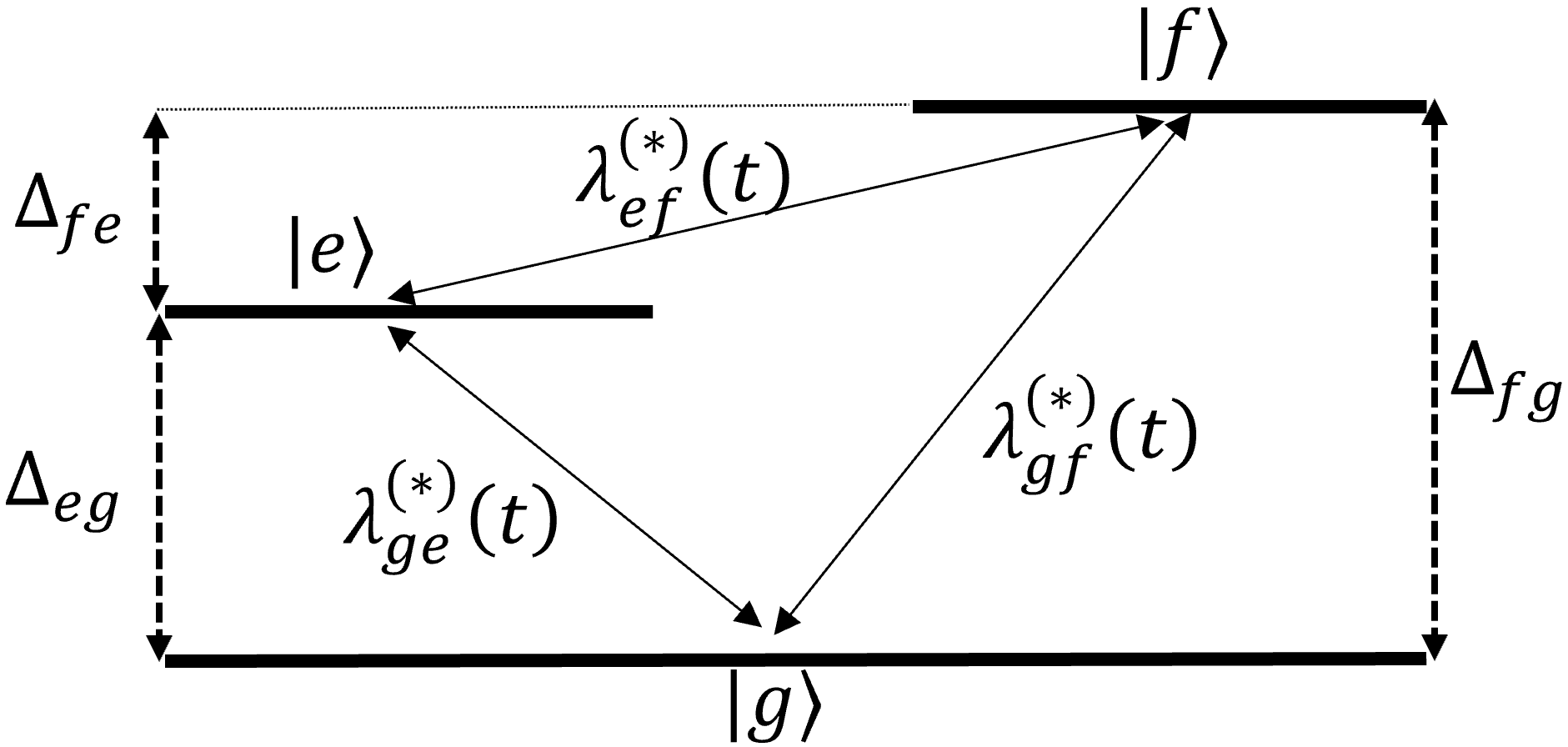
Figure 18: A three-level toy model with pairwise time-dependent interaction. Leakage may occur both directly (first order) but also via in-between transitions (higher order).

The interaction-frame Hamiltonian $\hat{\mathcal{H}}_{\text{I}}(t)\equiv e^{i\hat{\mathcal{H}}_{0}t}\hat{\mathcal{H}}_{\text{int}}(t)e^{-i\hat{\mathcal{H}}_{0}t}$ is found as

$$\hat{\mathcal{H}}_{\text{I}}(t)=\begin{bmatrix}0&\lambda_{\text{ge}}^{*}(t)e^{-i\Delta_{\text{eg}}t}&\lambda_{\text{gf}}^{*}(t)e^{-i\Delta_{\text{fg}}t}\\ \lambda_{\text{ge}}(t)e^{i\Delta_{\text{eg}}t}&0&\lambda_{\text{ef}}^{*}(t)e^{-i\Delta_{\text{fe}}t}\\ \lambda_{\text{gf}}(t)e^{i\Delta_{\text{fg}}t}&\lambda_{\text{ef}}(t)e^{i\Delta_{\text{fe}}t}&0\end{bmatrix}\;,$$ (117)

where for simplicity we have defined $\Delta_{\text{fe}}\equiv\Delta_{\text{fg}}-\Delta_{\text{eg}}$. The time-evolution operator in the interaction frame reads

$$\hat{U}_{I}(t,0)=\mathbb{T}\exp\left[-i\int_{0}^{t}dt^{\prime}\hat{\mathcal{H}}_{I}(t^{\prime})\right]\;,$$ (118)

where $\mathbb{T}$ is the time-ordering operator. In the Magnus method, we solve for the generator of $\hat{U}_{I}(t,0)$ perturbatively as

$$\begin{split}\hat{U}_{I}(t,0)&\equiv e^{-i\hat{K}(t,0)}=\hat{I}-i\hat{K}_{1}(t,0)\\ &-i\hat{K}_{2}(t,0)-\frac{1}{2}\hat{K}_{1}^{2}(t,0)+O\left(\hat{\mathcal{H}}_{I}^{3}(t)\right)\;,\end{split}$$ (119a)

where $$\hat{K}_{n}(t,0) n$$ is the th order solution for the generator. Up to the 2nd order we find Blanes_Pedagogical_2010

$$\hat{K}_{1}(t,0)\equiv\int_{0}^{t}dt^{\prime}\hat{\mathcal{H}}_{I}(t^{\prime})\;,$$ (119b)

$$\hat{K}_{2}(t,0)\equiv-\frac{i}{2}\int_{0}^{t}dt^{\prime}\int_{0}^{t^{\prime}}dt^{\prime\prime}\left[\hat{\mathcal{H}}_{I}(t^{\prime}),\hat{\mathcal{H}}_{I}(t^{\prime\prime})\right]\;.$$ (119c)

Using Eqs. (119a)–(119c), we calculate the transition probabilities. For instance, the probability amplitude for $\ket{g}\rightarrow\ket{f}$ at $t=\tau$ reads

$$\begin{split}&\bra{\text{f}}\hat{U}_{I}(\tau,0)\ket{g}=-i\int_{0}^{\tau}dt^{\prime}\lambda_{\text{gf}}(t^{\prime})e^{i\Delta_{\text{fg}}t^{\prime}}\\ &-\frac{1}{2}\left(\int_{0}^{\tau}dt^{\prime}\lambda_{\text{ef}}(t^{\prime})e^{i\Delta_{\text{fe}}t^{\prime}}\right)\left(\int_{0}^{\tau}dt^{\prime}\lambda_{\text{ge}}(t^{\prime})e^{i\Delta_{\text{eg}}t^{\prime}}\right)\\ &+\frac{1}{2}\int_{0}^{\tau}dt^{\prime}\int_{0}^{t^{\prime}}dt^{\prime\prime}\lambda_{\text{ge}}(t^{\prime})\lambda_{\text{ef}}(t^{\prime\prime})e^{i\Delta_{\text{eg}}t^{\prime}}e^{i\Delta_{\text{fe}}t^{\prime\prime}}\\ &-\frac{1}{2}\int_{0}^{\tau}dt^{\prime}\int_{0}^{t^{\prime}}dt^{\prime\prime}\lambda_{\text{ef}}(t^{\prime})\lambda_{\text{ge}}(t^{\prime\prime})e^{i\Delta_{\text{fe}}t^{\prime}}e^{i\Delta_{\text{eg}}t^{\prime\prime}}\;.\end{split}$$ (120)

which is a sum over all possible paths connecting states $\ket{g}$ and $\ket{f}$ either as a result of a direct interaction (first order) or through intermediate states (second order and higher). Other transitions have the same generic form.

According to Eq. (120), leakage occurs when the pulse spectrum has a non-negligible overlap with system transition frequencies. For instance, the first order term in Eq. (120) can be expressed in frequency domain as

$$\begin{split}&-i\int_{0}^{\tau}dt^{\prime}\lambda_{\text{gf}}(t^{\prime})e^{i\Delta_{\text{fg}}t^{\prime}}=\\ &-\int_{-\infty}^{\infty}\frac{d\omega^{\prime}}{2\pi}\frac{\tilde{\lambda}_{\text{gf}}(\omega^{\prime})}{\omega^{\prime}+\Delta_{\text{fg}}}\left[e^{i\Delta_{\text{fg}}\tau}-1\right]\;.\end{split}$$ (121)

In Sec. IV of the main text, we employ this fact to explain leakage to specific high-excitation qubit states in the parameter space of the RIP gate.

Appendix I Leakage error

Here we show that the average error of an arbitrary quantum operation has an approximate lower bounded set by the corresponding average leakage probability Wood_Quantification_2018 . Our assumption is that the physical evolution occurs in an extended D-dimensional Hilbert space, while the intended operation is defined over a d-dimensional subspace.

We employ projection operators $\hat{P}$ and $\hat{Q}$, onto the computational and leakage subspaces respectively, that satisfy

$$\begin{split}&\hat{P}^{2}=\hat{P}\;,\quad\quad\ \hat{Q^{2}}=\hat{Q}\;,\\ &\hat{P}+\hat{Q}=\hat{I}\;,\quad\hat{P}\hat{Q}=\hat{Q}\hat{P}=0\;.\end{split}$$ (122)

We then rewrite the overall time-evolution as

$$\begin{split}\hat{U}&=(\hat{P}+\hat{Q})\hat{U}(\hat{P}+\hat{Q})\\ &=\hat{P}\hat{U}\hat{P}+\hat{P}\hat{U}\hat{Q}+\hat{Q}\hat{U}\hat{P}+\hat{Q}\hat{U}\hat{Q}\;,\end{split}$$ (123)

where the first term provides the intended reduced operation (not necessarily unitary) in the computational subspace as

$$\hat{U}_{r}\equiv\hat{P}\hat{U}\hat{P}\;.$$ (124)

We assume the system starts in the computational subspace with initial state $\ket{\Psi_{s}}$ and the final state is obtained as $\ket{\Psi_{f}}\equiv\hat{U}\ket{\Psi_{s}}$. The corresponding leakage probability reads

$$p_{L,\Psi_{s}}\equiv\bra{\Psi_{f}}\hat{Q}^{{\dagger}}\hat{Q}\ket{\Psi_{f}}=\bra{\Psi_{s}}\hat{U}^{{\dagger}}\hat{Q}\hat{U}\ket{\Psi_{s}}\;.$$ (125)

Accordingly, we can define an average leakage probability by tracing over all possible initial states in the computational subspace as

$$\bar{p}_{L}\equiv\frac{1}{d}\operatorname{Tr}\left(\hat{P}\hat{U}^{{\dagger}}\hat{Q}\hat{U}\hat{P}\right)\;.$$ (126)

In Eq. (126), the trace is defined over the extended Hilbert space, explaining the need for additional $\hat{P}$ projections.

Average gate fidelity between the reduced operation $\hat{U}_{r}$ and the ideal (intended) gate operation $\hat{U}_{i}$ can be obtained as Pedersen_Fidelity_2007

$$\bar{F}(\hat{U}_{r},\hat{U}_{i})\equiv\frac{\operatorname{Tr}\left(\hat{U}_{r}\hat{U}_{r}^{{\dagger}}\right)}{d(d+1)}+\frac{\left|\operatorname{Tr}\left(\hat{U}_{r}^{{\dagger}}\hat{U}_{i}\right)\right|^{2}}{d(d+1)}\;.$$ (127)

The first term in Eq. (127) captures the infidelity due to $\hat{U}_{r}$ not being unitary, which e.g. can be caused by leakage, while the second term captures the infidelity as a result of deviation between the reduced physical and ideal operations. In the following, we derive a rather simple relation between the average leakage probability (126) and average fidelity (127).

Employing Eqs. (122)–(124) and the cyclic property of the trace operation we can write

$$\begin{split}\operatorname{Tr}\left(\hat{U}_{r}\hat{U}_{r}^{{\dagger}}\right)&=\operatorname{Tr}\left(\hat{P}\hat{U}\hat{P}\hat{P}^{{\dagger}}\hat{U}^{{\dagger}}\hat{P}^{{\dagger}}\right)\\ &=\operatorname{Tr}\left(\hat{P}\hat{U}^{{\dagger}}\hat{P}\hat{U}\hat{P}\right)\\ &=\operatorname{Tr}\left(\hat{P}\hat{U}^{{\dagger}}(\hat{I}-\hat{Q})\hat{U}\hat{P}\right)\\ &=\operatorname{Tr}\left(\hat{P}\hat{U}^{{\dagger}}\hat{U}\hat{P}\right)-\operatorname{Tr}\left(\hat{P}\hat{U}\hat{Q}\hat{U}^{{\dagger}}\hat{P}\right)\\ &=\operatorname{Tr}\left(\hat{P}\right)-\operatorname{Tr}\left(\hat{P}\hat{U}\hat{Q}\hat{U}^{{\dagger}}\hat{P}\right)\;.\end{split}$$ (128)

Comparing Eq. (128) with the average leakage probability (126) and using $\operatorname{Tr}(\hat{P})=d$ we find

$$\operatorname{Tr}\left(\hat{U}_{r}\hat{U}_{r}^{{\dagger}}\right)=d(1-\bar{p}_{L})\;.$$ (129)

Equation (129) shows that the amount by which the reduced operation is non-unitary is proportional to the average leakage probability.

Knowledge of the average leakage probability is not sufficient for finding an estimate for the second term in Eq. (127). This is dependent on the underlying noise model that sets the relation between $\hat{U}_{r}$ and $\hat{U}_{i}$ (see Ref. Wood_Quantification_2018 for a detailed analysis). If we assume that $\hat{U}_{r}\propto\hat{U}_{i}$, based on Eq. (129) and the fact that $\hat{U}_{i}$ is unitary, we can deduce

$$\hat{U}_{r}\approx\sqrt{1-\bar{p}_{L}}\hat{U}_{i}\;.$$ (130)

Replacing Eq. (130) in the second term of Eq. (127) we find

$$\left|\operatorname{Tr}\left(\hat{U}_{r}^{{\dagger}}\hat{U}_{i}\right)\right|^{2}\approx d^{2}(1-\bar{p}_{L})\;.$$ (131)

Substituting Eqs. (129) and (131) into Eq. (127) yields

$$\begin{split}\bar{F}(\hat{U}_{r},\hat{U}_{i})&\approx\frac{1}{d(d+1)}\left[d(1-\bar{p}_{L})+d^{2}(1-\bar{p}_{L})\right]\\ &=1-\bar{p}_{L}\;.\end{split}$$ (132)

In summary, the average leakage probability sets an approximate lower bound for the corresponding average error $\bar{E}(\hat{U}_{r},\hat{U}_{i})\equiv 1-\bar{F}(\hat{U}_{r},\hat{U}_{i})$ as

$$\bar{E}(\hat{U}_{r},\hat{U}_{i})\gtrsim\bar{p}_{L}\;.$$ (133)

In the case of a two-qubit gate operation with $d=4$ and target error given by $\bar{E}(\hat{U}_{r},\hat{U}_{i})\leq 10^{-4}$, the average leakage probability must be kept below $\bar{p}_{L}\lesssim 10^{-4}$ as well.

Appendix J Numerical methods

Numerical simulations for leakage in Sec. IV were performed using the Schrödinger equation solver of the QuTiP package Johansson_Qutip_2012 , called sesolve, plus standard Python scientific computing dependencies such as numpy Harris_Array_2020 , scipy Virtanen_Scipy_2020 and pandas Mckinney_Pandas_2011 . Simulations were run in parallel over multiple servers: 3 servers with 48 cores and 196 GB of RAM, 1 server with 56 cores and 248 GB of RAM, plus a controlling server with 4 cores and 8 GB of RAM. These servers were running Red Hat Enterprise Linux 7 and IBM Spectrum LSF for job queuing. Simulations were managed using dask and dask_jobqueue dask_2016 to submit jobs to LSF. QuTiP, dask_jobqueue, and their dependencies were managed using conda conda_2017 and the packages provided by conda-forge conda_forge_community_2015_4774216 . The servers were provisioned on the IBM Cloud by the IBM Research Hybrid Cloud service.

References

- [1] Daniel Sank, Zijun Chen, Mostafa Khezri, J. Kelly, R. Barends, B. Campbell, Y. Chen, B. Chiaro, A. Dunsworth, A. Fowler, E. Jeffrey, E. Lucero, A. Megrant, J. Mutus, M. Neeley, C. Neill, P. J. J. O’Malley, C. Quintana, P. Roushan, A. Vainsencher, T. White, J. Wenner, Alexander N. Korotkov, and John M. Martinis. Measurement-induced state transitions in a superconducting qubit: Beyond the rotating wave approximation. Phys. Rev. Lett., 117:190503, Nov 2016.
- [2] Vincent Bouchiat, D Vion, Ph Joyez, D Esteve, and MH Devoret. Quantum coherence with a single cooper pair. Physica Scripta, 1998(T76):165, 1998.
- [3] Yu Nakamura, Yu A Pashkin, and JS Tsai. “coherent control of macroscopic quantum states in a single-cooper-pair box”. Nature, 398(6730):786–788, 1999.
- [4] Jonathan R Friedman, Vijay Patel, Wei Chen, SK Tolpygo, and James E Lukens. Quantum superposition of distinct macroscopic states. nature, 406(6791):43–46, 2000.
- [5] Yuriy Makhlin, Gerd SchĂśn, and Alexander Shnirman. Quantum-state engineering with Josephson-junction devices. Rev. Mod. Phys., 73(2):357–400, May 2001.
- [6] Caspar H Van Der Wal, ACJ Ter Haar, FK Wilhelm, RN Schouten, CJPM Harmans, TP Orlando, Seth Lloyd, and JE Mooij. Quantum superposition of macroscopic persistent-current states. Science, 290(5492):773–777, 2000.
- [7] John M Martinis, S Nam, J Aumentado, and C Urbina. Rabi oscillations in a large josephson-junction qubit. Physical Review Letters, 89(11):117901, 2002.
- [8] Alexandre Blais, Ren-Shou Huang, Andreas Wallraff, S. M. Girvin, and R. J. Schoelkopf. “cavity quantum electrodynamics for superconducting electrical circuits: An architecture for quantum computation”. Phys. Rev. A, 69:062320, Jun 2004.
- [9] Andreas Wallraff, David I Schuster, Alexandre Blais, Luigi Frunzio, R-S Huang, Johannes Majer, Sameer Kumar, Steven M Girvin, and Robert J Schoelkopf. “strong coupling of a single photon to a superconducting qubit using circuit quantum electrodynamics”. Nature, 431(7005):162–167, 2004.
- [10] Jens Koch, Terri M Yu, Jay M Gambetta, Andrew A Houck, David I Schuster, Joseph Majer, Alexandre Blais, Michel H Devoret, Steven M Girvin, and Robert J Schoelkopf. “charge-insensitive qubit design derived from the Cooper pair box”. Phys. Rev. A, 76(4):042319, October 2007.
- [11] Johannes Majer, Jerry M Chow, Jay M Gambetta, Jens Koch, Blake R Johnson, Joseph A Schreier, Luigi Frunzio, David I Schuster, Andrew A Houck, Andreas Wallraff, et al. “coupling superconducting qubits via a cavity bus”. Nature, 449(7161):443–447, 2007.
- [12] Peter W Shor. “algorithms for quantum computation: Discrete logarithms and factoring”. In Foundations of Computer Science, 1994 Proceedings., 35th Annual Symposium on, pages 124–134. IEEE, 1994.
- [13] David P DiVincenzo. “quantum computation”. Science, 270(5234):255–261, 1995.
- [14] Adriano Barenco, Charles H Bennett, Richard Cleve, David P DiVincenzo, Norman Margolus, Peter Shor, Tycho Sleator, John A Smolin, and Harald Weinfurter. “elementary gates for quantum computation”. Physical review A, 52(5):3457, 1995.
- [15] Andrew Steane. “quantum computing”. Reports on Progress in Physics, 61(2):117, 1998.
- [16] Peter W Shor. “quantum computing”. Documenta Mathematica, 1(1000):1, 1998.
- [17] Michael A Nielsen and Isaac Chuang. “Quantum computation and quantum information”. American Association of Physics Teachers, 2002.
- [18] Peter W Shor. “fault-tolerant quantum computation”. In Proceedings of 37th conference on foundations of computer science, pages 56–65. IEEE, 1996.
- [19] Daniel Gottesman. “theory of fault-tolerant quantum computation”. Physical Review A, 57(1):127, 1998.
- [20] Alexei Yu Kitaev. “fault-tolerant quantum computation by anyons”. Annals of Physics, 303(1):2–30, 2003.
- [21] Robert Raussendorf and Jim Harrington. “fault-tolerant quantum computation with high threshold in two dimensions”. Physical review letters, 98(19):190504, 2007.
- [22] Jay M Gambetta, Jerry M Chow, and Matthias Steffen. “building logical qubits in a superconducting quantum computing system”. npj Quantum Information, 3(1):1–7, 2017.
- [23] GS Paraoanu. “microwave-induced coupling of superconducting qubits’. Physical Review B, 74(14):140504, 2006.
- [24] Chad Rigetti and Michel Devoret. “fully microwave-tunable universal gates in superconducting qubits with linear couplings and fixed transition frequencies”. Physical Review B, 81(13):134507, 2010.
- [25] Jerry M Chow, Jay M Gambetta, Andrew W Cross, Seth T Merkel, Chad Rigetti, and M Steffen. “microwave-activated conditional-phase gate for superconducting qubits”. New Journal of Physics, 15(11):115012, 2013.
- [26] Andrew W Cross and Jay M Gambetta. “optimized pulse shapes for a resonator-induced phase gate”. Physical Review A, 91(3):032325, 2015.
- [27] Hanhee Paik, A Mezzacapo, Martin Sandberg, DT McClure, B Abdo, AD Córcoles, O Dial, DF Bogorin, BLT Plourde, M Steffen, et al. “experimental demonstration of a resonator-induced phase gate in a multiqubit circuit-qed system”. Physical review letters, 117(25):250502, 2016.
- [28] Shruti Puri and Alexandre Blais. “high-fidelity resonator-induced phase gate with single-mode squeezing”. Phys. Rev. Lett., 116:180501, May 2016.
- [29] E. Knill, D. Leibfried, R. Reichle, J. Britton, R. B. Blakestad, J. D. Jost, C. Langer, R. Ozeri, S. Seidelin, and D. J. Wineland. “randomized benchmarking of quantum gates”. Phys. Rev. A, 77:012307, Jan 2008.
- [30] Easwar Magesan, J. M. Gambetta, and Joseph Emerson. “scalable and robust randomized benchmarking of quantum processes”. Phys. Rev. Lett., 106:180504, May 2011.
- [31] M. Matti Maricq. “application of average hamiltonian theory to the nmr of solids”. Phys. Rev. B, 25:6622–6632, Jun 1982.
- [32] T. P. Grozdanov and M. J. Raković. “quantum system driven by rapidly varying periodic perturbation”. Phys. Rev. A, 38:1739–1746, Aug 1988.
- [33] Saar Rahav, Ido Gilary, and Shmuel Fishman. “effective hamiltonians for periodically driven systems”. Physical Review A, 68(1):013820, 2003.
- [34] Mazyar Mirrahimi and Pierre Rouchon. “modeling and control of quantum systems”. Lecture notes, 2010.
- [35] Nathan Goldman and Jean Dalibard. “periodically driven quantum systems: effective hamiltonians and engineered gauge fields”. Physical review X, 4(3):031027, 2014.
- [36] Chiao-Hsuan Wang, Kyungjoo Noh, José Lebreuilly, SM Girvin, and Liang Jiang. “photon-number dependent hamiltonian engineering for cavities”. arXiv preprint arXiv:2009.07855, 2020.
- [37] Easwar Magesan and Jay M. Gambetta. “effective hamiltonian models of the cross-resonance gate”. Phys. Rev. A, 101:052308, May 2020.
- [38] Moein Malekakhlagh, Easwar Magesan, and David C. McKay. “first-principles analysis of cross-resonance gate operation”. Phys. Rev. A, 102:042605, Oct 2020.
- [39] John R Schrieffer and Peter A Wolff. “relation between the anderson and kondo hamiltonians”. Physical Review, 149(2):491, 1966.
- [40] Sergey Bravyi, David P DiVincenzo, and Daniel Loss. “schrieffer–wolff transformation for quantum many-body systems”. Annals of physics, 326(10):2793–2826, 2011.
- [41] Marin Bukov, Michael Kolodrubetz, and Anatoli Polkovnikov. “schrieffer-wolff transformation for periodically driven systems: Strongly correlated systems with artificial gauge fields”. Phys. Rev. Lett., 116:125301, Mar 2016.
- [42] Moein Malekakhlagh, Alexandru Petrescu, and Hakan E. Türeci. “lifetime renormalization of weakly anharmonic superconducting qubits. I. role of number nonconserving terms”. Phys. Rev. B, 101:134509, Apr 2020.
- [43] Alexandru Petrescu, Moein Malekakhlagh, and Hakan E. Türeci. “lifetime renormalization of driven weakly anharmonic superconducting qubits. II. the readout problem”. Phys. Rev. B, 101:134510, Apr 2020.
- [44] Vinay Tripathi, Mostafa Khezri, and Alexander N. Korotkov. “operation and intrinsic error budget of a two-qubit cross-resonance gate”. Phys. Rev. A, 100:012301, Jul 2019.
- [45] Jared B Hertzberg, Eric J Zhang, Sami Rosenblatt, Easwar Magesan, John A Smolin, Jeng-Bang Yau, Vivekananda P Adiga, Martin Sandberg, Markus Brink, Jerry M Chow, et al. “laser-annealing josephson junctions for yielding scaled-up superconducting quantum processors”. npj Quantum Information, 7(1):1–8, 2021.
- [46] Eric J Zhang, Srikanth Srinivasan, Neereja Sundaresan, Daniela F Bogorin, Yves Martin, Jared B Hertzberg, John Timmerwilke, Emily J Pritchett, Jeng-Bang Yau, Cindy Wang, et al. “high-fidelity superconducting quantum processors via laser-annealing of transmon qubits”. arXiv preprint arXiv:2012.08475, 2020.
- [47] Raphaël Lescanne, Lucas Verney, Quentin Ficheux, Michel H Devoret, Benjamin Huard, Mazyar Mirrahimi, and Zaki Leghtas. “escape of a driven quantum josephson circuit into unconfined states”. Physical Review Applied, 11(1):014030, 2019.
- [48] Lucas Verney, Raphaël Lescanne, Michel H Devoret, Zaki Leghtas, and Mazyar Mirrahimi. “structural instability of driven josephson circuits prevented by an inductive shunt”. Physical Review Applied, 11(2):024003, 2019.
- [49] F. Motzoi, J. M. Gambetta, P. Rebentrost, and F. K. Wilhelm. “simple pulses for elimination of leakage in weakly nonlinear qubits”. Phys. Rev. Lett., 103:110501, Sep 2009.
- [50] Jay M Gambetta, F Motzoi, ST Merkel, and Frank K Wilhelm. “analytic control methods for high-fidelity unitary operations in a weakly nonlinear oscillator”. Physical Review A, 83(1):012308, 2011.
- [51] Moein Malekakhlagh and Easwar Magesan. “mitigating off-resonant error in the cross-resonance gate”. arXiv preprint arXiv:2108.03223, 2021.
- [52] Moein Malekakhlagh, Alexandru Petrescu, and Hakan E. Türeci. “non-markovian dynamics of a superconducting qubit in an open multimode resonator”. Phys. Rev. A, 94:063848, Dec 2016.
- [53] Moein Malekakhlagh and Hakan E. Türeci. “origin and implications of an -like contribution in the quantization of circuit-qed systems”. Phys. Rev. A, 93:012120, Jan 2016.
- [54] Moein Malekakhlagh, Alexandru Petrescu, and Hakan E. Türeci. “cutoff-free circuit quantum electrodynamics”. Phys. Rev. Lett., 119:073601, Aug 2017.
- [55] Nicolas Didier, Eyob A Sete, Marcus P da Silva, and Chad Rigetti. “analytical modeling of parametrically modulated transmon qubits”. Physical Review A, 97(2):022330, 2018.
- [56] Simon E. Nigg, Hanhee Paik, Brian Vlastakis, Gerhard Kirchmair, S. Shankar, Luigi Frunzio, M. H. Devoret, R. J. Schoelkopf, and S. M. Girvin. “black-box superconducting circuit quantization”. Phys. Rev. Lett., 108:240502, Jun 2012.
- [57] Zlatko K. Minev, Zaki Leghtus, Shantanu O. Mundhada, Lysander Christakis, Ion M. Pop, and Michel H. Devoret. “energy-participation quantization of josephson circuits”. arXiv preprint arXiv:2010.00620, 2020.
- [58] Ahmed Jellal, Michael Schreiber, and El Hassan El Kinani. “two coupled harmonic oscillators on noncommutative plane”. International Journal of Modern Physics A, 20(07):1515–1529, 2005.
- [59] Abdeldjalil Merdaci and Ahmed Jellal. “entanglement in three coupled harmonic oscillators”. Physics Letters A, 384(6):126134, 2020.
- [60] Rok Zitko. “sneg-mathematica package for symbolic calculations with second-quantization-operator expressions”. arXiv preprint arXiv:1105.4697, 2011.
- [61] PD Drummond and CW Gardiner. “generalised p-representations in quantum optics”. Journal of Physics A: Mathematical and General, 13(7):2353, 1980.
- [62] Alexandru Petrescu, Camille Le Calonnec, Catherine Leroux, Agustin Di Paolo, Pranav Mundada, Sara Sussman, Andrei Vrajitoarea, Andrew A Houck, and Alexandre Blais. “accurate methods for the analysis of strong-drive effects in parametric gates”. arXiv preprint arXiv:2107.02343, 2021.
- [63] M Pechal, S Berger, AA Abdumalikov Jr, JM Fink, Jonas A Mlynek, L Steffen, Andreas Wallraff, and Stefan Filipp. “geometric phase and nonadiabatic effects in an electronic harmonic oscillator”. Physical Review Letters, 108(17):170401, 2012.
- [64] Arno Bohm, Ali Mostafazadeh, Hiroyasu Koizumi, Qian Niu, and Josef Zwanziger. “The Geometric phase in quantum systems: foundations, mathematical concepts, and applications in molecular and condensed matter physics”. Springer Science & Business Media, 2013.
- [65] Yu Chen, C Neill, P Roushan, N Leung, M Fang, R Barends, J Kelly, B Campbell, Z Chen, B Chiaro, et al. “qubit architecture with high coherence and fast tunable coupling”. Physical review letters, 113(22):220502, 2014.
- [66] Pranav Mundada, Gengyan Zhang, Thomas Hazard, and Andrew Houck. “suppression of qubit crosstalk in a tunable coupling superconducting circuit”. Physical Review Applied, 12(5):054023, 2019.
- [67] Abhinav Kandala, Ken X. Wei, Srikanth Srinivasan, Easwar Magesan, Santino Carnevale, George A. Keefe, David Klaus, Oliver Dial, and David C. McKay. “demonstration of a high-fidelity cnot for fixed-frequency transmons with engineered suppression”. arXiv preprint quant-ph/2011.07050, 2020.
- [68] Jaseung Ku, Xuexin Xu, Markus Brink, David C. McKay, Jared B. Hertzberg, Mohammad H. Ansari, and B. L. T. Plourde. “suppression of unwanted interactions in a hybrid two-qubit system”. Phys. Rev. Lett., 125:200504, Nov 2020.
- [69] KX Wei, E Magesan, I Lauer, S Srinivasan, DF Bogorin, S Carnevale, GA Keefe, Y Kim, D Klaus, W Landers, et al. “quantum crosstalk cancellation for fast entangling gates and improved multi-qubit performance”. arXiv preprint arXiv:2106.00675, 2021.
- [70] Bradley K Mitchell, Ravi K Naik, Alexis Morvan, Akel Hashim, John Mark Kreikebaum, Brian Marinelli, Wim Lavrijsen, Kasra Nowrouzi, David I Santiago, and Irfan Siddiqi. “hardware-efficient microwave-activated tunable coupling between superconducting qubits”. arXiv preprint arXiv:2105.05384, 2021.
- [71] Muir Kumph, James J Raftery, Will Shanks, Aaron Finck, John Blair, George Keefe, Santino Carnevale, Vincent Arena, Shawn Hall, Dave Klaus, and Oliver E Dial. “novel coupling for rip gate devices”. Bulletin of the American Physical Society, 2021.
- [72] Jared Hertzberg, Sami Rosenblatt, Jose Chavez, Easwar Magesan, John Smolin, Jeng-Bang Yau, Vivekananda Adiga, Markus Brink, Eric Zhang, Jason Orcutt, et al. “effects of qubit frequency crowding on scalable quantum processors”. Bulletin of the American Physical Society, 2020.
- [73] Wilhelm Magnus. “on the exponential solution of differential equations for a linear operator”. Communications on pure and applied mathematics, 7(4):649–673, 1954.
- [74] Sergio Blanes, Fernando Casas, Jose-Angel Oteo, and José Ros. “the magnus expansion and some of its applications”. Physics reports, 470(5-6):151–238, 2009.
- [75] Sergio Blanes, Fernando Casas, JA Oteo, and J Ros. “a pedagogical approach to the magnus expansion”. European journal of physics, 31(4):907, 2010.
- [76] Spectrum of an isolated transmon, based on , is periodic with respect to the gate charge [10]. However, a charge-charge coupling of the form to a resonator mode breaks such a translational symmetry. Our numerical simulations show that for experimentally relevant values of qubit-resonator coupling (full dispersive shift of the order of -5 MHz), the deviation in the spectrum and also the corresponding deviation in the qubit-resonator leakage is small under . Moreover, the result is approximately symmetric with respect to , Therefore, in Fig. 9, we have presented the dependence of leakage on the approximately unique interval of .
- [77] Christopher J. Wood and Jay M. Gambetta. “quantification and characterization of leakage errors”. Phys. Rev. A, 97:032306, Mar 2018.
- [78] Jay Gambetta, Alexandre Blais, D. I. Schuster, A. Wallraff, L. Frunzio, J. Majer, M. H. Devoret, S. M. Girvin, and R. J. Schoelkopf. “qubit-photon interactions in a cavity: Measurement-induced dephasing and number splitting”. Phys. Rev. A, 74:042318, Oct 2006.
- [79] E. M. Purcell, H. C. Torrey, and R. V. Pound. “resonance absorption by nuclear magnetic moments in a solid”. Phys. Rev., 69:37–38, Jan 1946.
- [80] Edward Mills Purcell. Spontaneous emission probabilities at radio frequencies. In Confined Electrons and Photons, pages 839–839. Springer, 1995.
- [81] A. A. Houck, J. A. Schreier, B. R. Johnson, J. M. Chow, Jens Koch, J. M. Gambetta, D. I. Schuster, L. Frunzio, M. H. Devoret, S. M. Girvin, and R. J. Schoelkopf. “controlling the spontaneous emission of a superconducting transmon qubit”. Phys. Rev. Lett., 101:080502, Aug 2008.
- [82] Sarah Sheldon, Easwar Magesan, Jerry M Chow, and Jay M Gambetta. “procedure for systematically tuning up cross-talk in the cross-resonance gate”. Physical Review A, 93(6):060302, 2016.
- [83] Neereja Sundaresan, Isaac Lauer, Emily Pritchett, Easwar Magesan, Petar Jurcevic, and Jay M Gambetta. “reducing unitary and spectator errors in cross resonance with optimized rotary echoes”. PRX Quantum, 1(2):020318, 2020.
- [84] Petar Jurcevic, Ali Javadi-Abhari, Lev S Bishop, Isaac Lauer, Daniela F Bogorin, Markus Brink, Lauren Capelluto, Oktay Günlük, Toshinari Itoko, Naoki Kanazawa, et al. “demonstration of quantum volume 64 on a superconducting quantum computing system”. Quantum Science and Technology, 6(2):025020, 2021.
- [85] Maxime Boissonneault, JM Gambetta, and Alexandre Blais. Nonlinear dispersive regime of cavity qed: The dressed dephasing model. Physical Review A, 77(6):060305, 2008.
- [86] Maxime Boissonneault, Jay M Gambetta, and Alexandre Blais. “dispersive regime of circuit qed: Photon-dependent qubit dephasing and relaxation rates”. Phys. Rev. A, 79:013819, Jan 2009.
- [87] ZK Minev, SO Mundhada, Shyam Shankar, Philip Reinhold, Ricardo Gutiérrez-Jáuregui, RJ Schoelkopf, Mazyar Mirrahimi, HJ Carmichael, and MH Devoret. “to catch and reverse a quantum jump mid-flight”. Nature, 570:200–204, 2019.
- [88] Ryo Hanai, Alexander McDonald, and Aashish Clerk. “intrinsic mechanisms for drive-dependent purcell decay in superconducting quantum circuits”. arXiv preprint arXiv:2106.05179, 2021.
- [89] Mazyar Mirrahimi, Zaki Leghtas, Victor V Albert, Steven Touzard, Robert J Schoelkopf, Liang Jiang, and Michel H Devoret. “dynamically protected cat-qubits: a new paradigm for universal quantum computation”. New Journal of Physics, 16(4):045014, 2014.
- [90] Zaki Leghtas, Steven Touzard, Ioan M Pop, Angela Kou, Brian Vlastakis, Andrei Petrenko, Katrina M Sliwa, Anirudh Narla, Shyam Shankar, Michael J Hatridge, et al. “confining the state of light to a quantum manifold by engineered two-photon loss”. Science, 347(6224):853–857, 2015.
- [91] Alexander Grimm, Nicholas E Frattini, Shruti Puri, Shantanu O Mundhada, Steven Touzard, Mazyar Mirrahimi, Steven M Girvin, Shyam Shankar, and Michel H Devoret. “stabilization and operation of a kerr-cat qubit”. Nature, 584(7820):205–209, 2020.
- [92] Maurice A De Gosson. “Symplectic geometry and quantum mechanics”, volume 166. Springer Science & Business Media, 2006.
- [93] Maurice A De Gosson. “Symplectic methods in harmonic analysis and in mathematical physics”, volume 7. Springer Science & Business Media, 2011.
- [94] Line Hjortshøj Pedersen, Niels Martin Møller, and Klaus Mølmer. “fidelity of quantum operations”. Physics Letters A, 367(1-2):47–51, 2007.
- [95] J Robert Johansson, Paul D Nation, and Franco Nori. “qutip: An open-source python framework for the dynamics of open quantum systems”. Computer Physics Communications, 183(8):1760–1772, 2012.
- [96] Charles R Harris, K Jarrod Millman, Stéfan J van der Walt, Ralf Gommers, Pauli Virtanen, David Cournapeau, Eric Wieser, Julian Taylor, Sebastian Berg, Nathaniel J Smith, et al. “array programming with numpy”. Nature, 585(7825):357–362, 2020.
- [97] Pauli Virtanen, Ralf Gommers, Travis E Oliphant, Matt Haberland, Tyler Reddy, David Cournapeau, Evgeni Burovski, Pearu Peterson, Warren Weckesser, Jonathan Bright, et al. “scipy 1.0: fundamental algorithms for scientific computing in python”. Nature methods, 17(3):261–272, 2020.
- [98] Wes McKinney et al. “pandas: a foundational python library for data analysis and statistics”. Python for high performance and scientific computing, 14(9):1–9, 2011.
- [99] Dask Development Team. “Dask: Library for dynamic task scheduling”, 2016.
- [100] Anaconda, Inc. “Conda”, 2017.
- [101] conda-forge community. “the conda-forge project: Community-based software distribution built on the conda package format and ecosystem”, July 2015.