Highly Optimized Full-Core Reactor Simulations on Summit

Abstract

Nek5000/RS is a highly-performant open-source spectral element code for simulation of incompressible and low-Mach fluid flow, heat transfer, and combustion with a particular focus on turbulent flows in complex domains. It is based on high-order discretizations that realize the same (or lower) cost per gridpoint as traditional low-order methods. State-of-the-art multilevel preconditioners, efficient high-order time-splitting methods, and runtime-adaptive communication strategies are built on a fast OCCA-based kernel library, libParanumal, to provide scalability and portability across the spectrum of current and future high-performance computing platforms. On Summit, Nek5000/RS has recently achieved an milestone in the simulation of nuclear reactors: the first full-core computational fluid dynamics simulations of reactor cores, including pebble beds with $>$ 350,000 pebbles and 98M elements advanced in less than 0.25 seconds per Navier-Stokes timestep. With carefully tuned algorithms, it is possible to simulate a single flow-through time for a full reactor core in less than six hours on all of Summit.

1 Introduction

We present first-ever large-eddy simulation of full reactor cores. Our elliptic-operator kernels sustain $>$ 1 TFLOPS FP64 on V100s and demonstarte 80% parallel efficiency at $\approx 2.5$M gridpoints per V100 with 0.1–0.25 second timesteps for Navier-Stokes problems using 50–60B gridpoints on Summit. We mesaure time-to-solution and provide scalability studies on full-scale system of Summit. We demonstrate four-fold reduction in solution time through algorithmic advances based on our semi-implicit spectral element method (SEM) approach with advanced preconditioning strategies utilizing mixed precision.

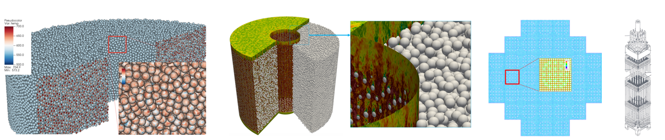
Figure 1: Reactor simulations of turbulent flow performed on OLCF/Summit (left to right): MOOSE-NekRS simulation of start-up transient for 127,602 pebbles, temperatures in K; full core with 352,625 pebbles using an all-hex mesh comprising $E$=98,782,067 elements of order $N=8$; full core with 37 assemblies of 17$\times$17 pin bundles using 1 billion elements of order $N=5$; cut-away illustration of 17x17 bundle.

We are interested in the modeling and simulation of nuclear reactor cores, one the historic challenges associated with computing from its onset Merzari et al. (2021a); Bajorek (2016). The numerical simulation of nuclear reactors is an inherently multi-physics problem involving fluid dynamics, heat transfer, radiation transport (neutrons) and material and structural dynamics.

In particular we will focus here on the modeling of turbulent heat and mass transfer in the core, which remains the most computationally expensive physics to be solved at the continuum level Grötzbach and Wörner (1999); Merzari et al. (2017). In fact, because of the complexity and range of scales involved in reactor cores ($~{}1\mu m-10m$), simplifications involving homogenization (e.g., treating the core effectively as porous medium) or Reynolds averaging have been historically necessary Novak et al. (2021); Cleveland and Greene (1986). Such approaches, while very powerful and useful for design, require modeling closures that are expensive or impossible to develop and validate, especially at the appropriate scale, and lead to design compromises in terms of operational margins and economics Roelofs (2018).

In the past 10 years, simulation on leadership computing platforms has been critical to improving informed analysis Merzari et al. (2020b). In fact, starting in 2009, turbulence-resolving simulations, such as direct numerical simulation (DNS) or wall-resolved large eddy simulation (LES), of small portions of the reactor core called fuel assemblies (e.g., $~{}100$ rods, $10cm$ tall) have emerged. These simulations have provided invaluable insight into the physics involved in turbulent heat and mass transfer in reactor cores. However, the simulation of a full reactor core has been elusive due to the sheer size of the system (e.g., $~{}10,000$ rods, 2–3m tall), limiting the use of such techniques, especially for multi-physics simulations that require full core analysis.

Given the increased interest in advanced carbon-free nuclear fission reactors worldwide, such turbulence-resolving full core simulations will be invaluable to provide benchmark datasets for improved reduced-resolution models (including advanced porous media models). This will in turn lead to reduced uncertainty, and ultimately to improved economics. In 2019 Merzari et al. (2020a) we provided a timeline for full-core LES calculations and we estimated that a full exascale machine would be necessary. Thanks to several major innovations in Nek5000/NekRS, this goal was recently achieved on pre-exascale machines. We present here the first full-core computational fluid dynamics (CFD) calculations to date.

In this article, we demonstrate that it is possible to realize a single flow-through-time in just six hours of wall-clock time when running on all of Summit (27648 NVIDIA V100s). It is thus realistic to expect that reactor designers could consider parametric analysis on future exascale platforms, which will be substantially larger than Summit.

To understand the transformative leap enabled by Nek5000/NekRS and in particular NekRS, it is instructive to examine coupled simulations in pebble beds. Before NekRS the largest pebble bed calculations in the literature involved of the order of $~{}1000$ pebbles with RANS Van Staden et al. (2018) and $~{}100$ pebbles with LES Yildiz et al. (2020). In this manuscript we describe calculations that reach over the active section of the full core for the Mark-I Flouride Cooled High Temperature Reactor ($352,625$ pebbles) Andreades et al. (2016).

Cardinal Merzari et al. (2021b) couples NekRS to OpenMC, a Monte Carlo solver for neutron transport, and to MOOSE, a multi-physics framework that has been used to solve the complex physics involved in fuel performance. The coupled simulations of the Mark-I reactor have been performed on Summit with 6 MPI ranks per node corresponding to the 6 GPUs on each node. NekRS simulates the flow and temperature distribution around the pebbles on the GPUs; OpenMC solves neutron transport on the CPU using 6 threads for each MPI rank; and MOOSE solves unsteady conduction in the fuel pebbles on the CPU. MOOSE can also incorporate more complex fuel performance models (BISON) including fission production and transport. Coupled simulations on Summit have been performed for pebble counts ranging from 11,145 pebbles on 100 nodes to 352,625 pebbles (full core) on 3000 nodes. In all cases, NekRS consumes $\approx$ 80% of the runtime. Figure 1(left) represents the temperature distribution inside the pebbles and on the surface during a heat-up transient (i.e., temperature starting from a constant temperature everywhere) for the 127,602 pebble case. These coupled simulations, which would have been considered impossible only a few years ago, demonstrate that the majority of the computational cost is in the thermal-fluids solve, which is the focus of this study.

2 Algorithms

Our focus is on the incompressible Navier-Stokes (NS) equations for velocity (${\bf u}$) and pressure ($p$),

$$\frac{D{\bf u}}{Dt}\!:=\!\frac{\partial{\bf u}}{\partial t}+{\bf u}\cdot\nabla{\bf u}\!=\!\frac{1}{Re}\nabla^{2}{\bf u}-\nabla p,\;\nabla\cdot{\bf u}=0,\;\;$$ (1)

where $Re=UL/\nu\gg 1$ is the Reynolds number based on flow speed $U$, length scale $L$, and viscosity $\nu$. (The equation for temperature is similar to (1) without the pressure, which makes it much simpler.) From a computational standpoint, the long-range coupling of the incompressibility constraint, $\nabla\cdot{\bf u}=0$, makes the pressure substep intrinsically communication intensive and a major focus of our effort as it consumes 60-80% of the run time.

NekRS is based on the spectral element method (SEM) Patera (1984), in which functions are represented as $N$th-order polynomials on each of $E$ elements, for a total mesh resolution of $n=EN^{3}$. While early GPU efforts for Nek5000 were on OpenACC ports Markidis et al. (2015) and Otten et al. (2016)(for NekCEM), NekRS originates from two code suites, Nek5000 Fischer et al. (2008) and libParanumal Świrydowicz et al. (2019); Karakus et al. (2019), which is a fast GPU-oriented library for high-order methods written in the open concurrent compute abstraction (OCCA) for cross-platform portability Medina et al. (2014).

The SEM offers many advantages for this class of problems. It accommodates body-fitted coordinates through isoparametric mappings domain from the reference element, ${\hat{\Omega}}:=[-1,1]^{3}$ to the individual (curvilinear-brick) elements $\Omega^{e}$. On ${\hat{\Omega}}$, solutions are represented in terms of $N$th-order tensor-product polynomials,

$$\left.{\bf u}({\bf x})\right|_{\Omega^{e}}=\sum_{i=0}^{N}\sum_{j=0}^{N}\sum_{k=0}^{N}{\bf u}_{ijk}^{e}\,h_{i}(r)\,h_{j}(s)\,h_{k}(t),$$ (2)

where the $h_{i}$s are stable nodal interpolants based on the Gauss-Lobatto-Legendre (GLL) quadrature points $(\xi_{i},\xi_{j},\xi_{j})\in{\hat{\Omega}}$ and ${\bf x}={\bf x}^{e}(r,s,t)$ on $\Omega^{e}$. This form allows all operator evaluations to be expressed as fast tensor contractions, which can be implemented as BLAS3 operations in only $O(N^{4})$ work and $O(N^{3})$ memory references Deville et al. (2002); Orszag (1980). This low complexity is in sharp contrast to the $O(N^{6})$ work and storage complexity of the traditional $p$-type FEM. Moreover, hexahdral (hex) element function evaluation is about six times faster per degree-of-freedom (dof) than tensor-based tetrahedal (tet) operator evaluation Moxey et al. (2020). By diagonalizing one direction at a time, the SEM structure admits fast block solvers for local Poisson problems in undeformed and (approximately) in deformed elements, which serve as local smoothers for $p$-multigrid (pMG) Lottes and Fischer (2005). $C^{0}$ continuity implies that the SEM is communication minimal: data exchanges have unit-depth stencils, independent of $N$. Finally, local $i$-$j$-$k$ indexing avoids much of the indirect addressing associated with fully unstructured approaches, such that high-order SEM implementations can realize significantly higher throughput (millions of dofs per second, MDOFS) than their low-order counterparts Fischer et al. (2020b).

The $O(N)$ computational intensity of the SEM brings direct benefits as its rapid convergence (exponential in $N$) allows one to accurately simulate flows with fewer gridpoints than lower-order discretizations. Turbulence DNS and LES require long-time simulations to reach statistically steady states and to gather statistics. For campaigns that can last weeks, turbulence simulations require not only performant implementations but also efficient discretizations that deliver high accuracy at low cost per gridpoint. Kreiss and Oliger Kreiss and Oliger (1972) noted that high-order methods are important when fast computers enable long integration times. To offset cumulative dispersion errors, $e(t)\sim Ct$, one must have $C\ll 1$ when $t\gg 1$. It is precisely in this regime that the asymptotic error behavior of the SEM, $C$=$O(h^{N})$, is manifest; it is more efficient to increase $N$ than to decrease the grid spacing, $h=O(E^{-\frac{1}{3}})$ (e.g., as in Fig. 2(d)).

High-order incompressible NS codes comparable in scalability to NekRS include Nektar Moxey et al. (2020), which employs the Nek5000 communication kernel, gslib and is based primarily on tets, libParanumalChalmers et al. (2020), NUMOGiraldo , deal.ii Arndt et al. (2017), and MFEM Anderson et al. (2020). The CPU-based kernel performance for the latter two is comparable to Nek5000 Fischer et al. (2020b). MFEM, which is a general purpose finite element library rather than a flow solver, has comparable GPU performance because of the common collaboration between the MFEM and Nek5000/RS teams that is part of DOE’s Center for Efficient Exascale Discretizations (CEED). NUMO, which targets ocean modeling, is also OCCA based. libParanumal, which is also under CEED, is at the cutting edge of GPU-based node performance on NVIDIA and AMD platforms Abdelfattah et al. (2020).

Regarding large-scale NS solutions on Summit, the closest point of comparison is the spectral (Fourier-box) code of Ravikumar et al. Ravikumar et al. (2019), which achieves 14.24 s/step for $n=18432^{3}$ and $P=18432$ V100s (3072 nodes)—a throughput rate $R$=23.6 MDOFS (millions of points-per-[second-GPU]). NekRS requires 0.24 s/step with $n=51$ billion and $P$=27648, for a throughput of $R$=7.62 MDOFS, for the full-reactor target problem of Fig. 1, which means that NekRS is within a factor of 3 of a dedicated spectral code. Traditionally, periodic-box codes, which do not store geometry, support general derivatives, or use iterative solvers, run 10-20$\times$ faster than general purpose codes. At this scale, however, the requisite all-to-alls for multidimensional FFTs of the spectral code place bisection-bandwidth burdens on the network that are not encountered with domain-decomposition approaches such as the SEM. We further note that $>1$ s/step is generally not practicable for production turbulence runs, which typically require $10^{5}$–$10^{6}$ timesteps.

Figure 2: Basis for NekRS: (a)–(b) Highly tuned OCCA-based Poisson kernel in libParanumal saturating the V100 roof-line, (b) Poisson operator kernel performance (no communication) as a function of $p$ ($\equiv N$) and $n=Ep^{3}$, (c) Nek5000 strong scaling to $>$ 1 million ranks, $n_{0.8}\approx 4000$ on Mira, (d) illustration of high-order benefits for the advection-dominated Walsh problem studied in Fischer et al. (2017). At engineering accuracy, the 8th-order expansion is significantly more accurate than the 2nd-order expansion for the same cost, $n$.

3 Implementation

Our decision to use OCCA was motivated by the need to port fast implementations to multiple-node architectures featuring Cuda, HIP, OpenMP, etc., without major revisions to code structure. Extensive tuning is required, which has been addressed in libParanumal (e.g., Świrydowicz et al. (2019); Fischer et al. (2020b)). Figures 2(a) and (b) show the performance of libParanumal on a single NVIDIA V100 for the local spectral element Poisson operator (without communication) as a function of kernel tuning (described in Fischer et al. (2020b)), polynomial order $p$ ($\equiv N$), and problem size $n$. We see that the performance saturates at the roofline for all cases when $E=4096$ in (a) and at $n\approx$ 250,000 for $p=$7–8 in (b). As we discuss in the sequel, because of communication overhead, we need $n/P\approx$ 2–3 million to sustain 80% parallel efficiency in the full Navier–Stokes case on Summit, where $P$ is the number of V100s employed in the simulation.

NekRS is based on libParanumal and leverages several of its high-performance kernels, including features such as overlapped communication and computation. It also inherits decades of development work from Nek5000, which has scaled to millions of ranks on Sequoia and Mira. As shown in Fig. 2(c), the 80% parallel efficiency mark for Nek5000 on Mira is at $n/P\approx 4000$ (where $P$ is the number of ranks), in keeping with the strong-scale analysis of Fischer et al. (2015) and the results obtained through cross-code comparisons in Fischer et al. (2020b) with the high-order deal.ii and MFEM libraries Arndt et al. (2017); Anderson et al. (2020).

Time advancement in NekRS is based on $k$th-order operator splitting ($k$=2 or 3) that decouples (1) into separate advection, pressure, and viscous substeps. The nonlinear advection terms are advanced by using backward differencing (BDF$k$) applied to the material derivative (e.g., $D{\bf u}/Dt\approx\frac{1}{2\Delta t}(3{\bf u}^{m}-4{\tilde{\bf u}}^{m-1}+{\tilde{\bf u}}^{m-2})$ for $k$=2), where values ${\tilde{\bf u}}^{m-j}$ along the characteristic are found by solving an explicit hyperbolic subproblem, $\frac{\partial{\bf w}}{\partial t}=-{\bf u}\cdot\nabla{\bf w}$, on $[t^{m-1},t^{m}]$ Patel et al. (2019); Maday et al. (1990). For stability (only), the variable-coefficient hyperbolic problem is dealiased by using Gauss–Legendre quadrature on $N_{q}>N$ quadrature points Malm et al. (2013). The characteristics approach allows for Courant numbers, CFL$:=\max_{{\bf x}\in\Omega}\Delta t|u_{i}/\Delta x_{i}|$, significantly larger than unity (CFL=2–4 is typical), thus reducing the required number of implicit Stokes (velocity-pressure) substeps per unit time interval.

Each Stokes substep requires the solution of 3 Helmholtz problems—one for each velocity component—which are diagonally dominant and efficiently treated by using Jacobi-preconditioned conjugate gradient iteration (Jacobi-PCG), and a Poisson solve for the pressure, which bypasses the need to track fast acoustic waves. Because of long-range interactions that make the problem communication intensive, the pressure Poisson solve is the dominant substep ($\approx$80% of runtime) in the NS time-advancement. To address this bottleneck, we use a variety of acceleration algorithms, including $p$-multigrid (pMG) preconditioning, projection-based solvers, and projection-based initial guesses.

The tensor-product structure of spectral elements makes implementation of pMG particularly simple. Coarse-to-fine interpolations are cast as efficient tensor contractions, ${\underline{u}}_{f}=({\hat{J}}\otimes{\hat{J}}\otimes{\hat{J}}){\underline{u}}_{c}$, where ${\hat{J}}$ is the 1D polynmial interpolation operator from the coarse GLL points to the fine GLL points. Like differentiation, interpolation is on the reference element, so only a single ${\hat{J}}$ matrix (of size $N+1$ or less) is needed for the entire domain, for each pMG level. Smoothers for pMG include Chebyshev-accelerated point-Jacobi, additive Schwarz Lottes and Fischer (2005), and Chebyshev-accelerated overlapping Schwarz. The Schwarz smoothers are implemented by solving local Poisson problems on domains extended into adjacent elements by one layer. Thus, for an $8\times 8\times 8$ brick ($N=7$), one solves a $10\times 10\times 10$ local problem, ${\tilde{A}}^{e}{\tilde{\underline{u}}}^{e}={\tilde{\underline{b}}}^{e}$, using fast diagonalization (FDM) Deville et al. (2002),

$${\tilde{\underline{u}}}^{e}=(S_{z}\otimes S_{y}\otimes S_{x})\Lambda^{-1}(S^{T}_{z}\otimes S^{T}_{y}\otimes S^{T}_{x}){\underline{b}}^{e},$$ (3)

$e=1,\dots,E,$ where each 1D matrix of eigenvectors, $S_{*}$, is $10\times 10$, and $\Lambda$ is a diagonal matrix with only $1,000$ nonzeros. The leading complexity is $\approx 12\times 10^{4}$ operations for the application of $S_{*}$ and $S_{*}^{T}$ (implemented as dgemm), with $\approx 2,000$ loads per element (for ${\underline{b}}^{e}$ and $\Lambda$). By constrast, $A^{e}$, if formed, would have 1 million nonzeros for each element, $\Omega^{e}$, which would make work and storage prohibitive. The fast low-storage tensor decomposition is critical to performance of the SEM, as first noted in the seminal paper of Orszag Orszag (1980). Note that the communication for the Schwarz solves is also very low. We exchange face data only to get the domain extensions—meaning 6 exchanges per element instead of 26. This optimization yields a 10% speedup in runs at the strong-scale limit. (We have also implemented a restricted additive Schwarz (RAS) variant, that does not require communication after the local solve, which cuts communication of the smoother by a factor of two.) Further preconditioner cost savings are realized by performing all steps of pMG in 32-bit arithmetic. On Summit, which has a limited number of NICs per node, this approach is advantageous because it reduces the off-node bandwidth demands by a factor of two.

Projection Is Key. For incompressible flows, the pressure evolves smoothly in time, and one can leverage this temporal regularity by projecting known components of the solution from prior timesteps. For any $n\times L$ subspace of ${{\rm l}\kern-1.49994pt{\rm R}}^{n}$ with $A$-orthonormal basis $P_{L}=[\underline{\tilde{p}}_{1}\dots\underline{\tilde{p}}_{L}]$, the best-fit approximation to the solution of $A{\underline{p}}^{m}={\underline{b}}^{m}$ is ${\bar{\underline{p}}}=P_{L}P_{L}^{T}{\underline{b}}^{m}$, which can be computed with a single all-reduce of length $L$ ($\lesssim 30$). The residual for the reduced problem $A{\delta{\underline{p}}}={\underline{b}}^{m}-A{\bar{\underline{p}}}$ has a significantly smaller norm such that relatively few GMRES iterations are required to compute ${\delta{\underline{p}}}$. We augment the space $P_{L+1}=[P_{L}\;\;{\delta{\underline{p}}}]$ after orthonormalizing ${\delta{\underline{p}}}$ against $P_{L}$ with one round of classical Gram-Schmidt orthogonalization, which requires only a single all-reduce. (This approach is stable because ${\delta{\underline{p}}}$ is nearly $A$-orthogonal to $P_{L}$.) In Sec. 7, we take $L_{\max}=30$ before restarting the approximation space, which yields a 1.7 speedup in NS solution time compared to $L$=0.

We remark that this projection algorithm is one of the few instances in distributed-memory computing where one can readily leverage the additional memory that comes with increasing the number of ranks, $P$. For low rank counts, one cannot afford $30$ vectors (each of size $n/P$ per rank) and must therefore take $L<30$, which results in suboptimal performance, as observed in the strong-scaling results of Sec.5. With increasing $P$, this solution algorithm improves because more memory is available for projection.

Subsequent to projection, we use (nonsymmetric) pMG-preconditioning applied to either flexible conjugate gradients (FlexCG) or GMRES. FlexCG uses a short recurrence and thus has lower memory and communication demands, whereas GMRES must retain $K$ vectors for $K$ iterations. With projection and a highly optimized preconditioner, however, we need only $K\lesssim 5$, which keeps both memory and work requirements low while retaining the optimal projective properties of GMRES. For the full NS solution with $n$=51B, GMRES outperforms FlexCG by about 3.3% on $P=27648$ V100s.

Autotuned Communication. On modern GPU platforms, one needs $n_{0.8}$$\approx$2.5 M points per GPU to realize $\approx$ 80% efficiency Fischer et al. (2020a). For $N=7$, this implies $E_{p}$$\approx$7300 elements per MPI rank (GPU), which provides significant opportunity for overlapping computation and communication because the majority of the elements are in the subdomain interior. NekRS supports several communication strategies for the SEM gather-scatter (gs) operation, which requires an exchange-and-sum of shared interface values: (a) pass-to-host, pack buffers, exchange; (b) pack-on-device, copy to host, exchange; and (c) pack-on-device, exchange via GPUDirect. They can be configured to overlap nonlocal gs communication with processor-internal gs updates and other local kernels (if applicable).

During gs-setup, the code runs a trial for each scenario and picks the fastest opetion. We note that processor adjacency is established in $\log P$ time through Nek5000’s gslib utility, which has scaled to billions of points on millions of ranks. The user (or code) simply provides a global ID for each vertex, and gslib identifies an efficient communication pattern to effect the requisite exchange. (For $n=51$B, setup time on all of Summit is 2.8 s.)

The computational mesh can have a profound influence on solution quality and on the convergence rate of the iterative solvers. We developed a code to generate high-quality meshes for random-packed spherical beds that was used in all pebble-bed cases shown. It is based on a tessellation of Voronoi cells with sliver removal to generate isotropic mesh distributions. The tessellated Voronoi facets are projected onto the sphere surfaces to sweep out hexahedral subdomains that are refined in the radial direction to provide boundary-layer resolution. This approach yields about 1/6 the number of elements as earlier tet-to-hex conversion approaches, which allows us to elevate the local approximation order for the same resolution while providing improved conditioning and less severe CFL constraints.

4 Performance Measurements

NekRS Timing Breakdown: n=51B, 2000 Steps
	pre-tuning		post-tuning
Operation	time (s)	%	time (s)	%
computation	1.19+03	100	5.47+02	100
advection	5.82+01	5	4.49+01	8
viscous update	5.38+01	5	5.98+01	11
pressure solve	1.08+03	90	4.39+02	80
precond.	9.29+02	78	3.67+02	67
coarse grid	5.40+02	45	6.04+01	11
projection	6.78+00	1	1.21+01	2
dotp	4.92+01	4	1.92+01	4

Table 1: Default NekRS statistics output, provided every 500 timesteps for each run, each user. This table shows results for the 352K pebble geometry of Fig. 1 on $P$=27648 V100s on Summit.

Our approach to performance assessment is both top-down and bottom-up. The top-down view comes from extensive experience on CPUs and GPUs of monitoring timing breakdowns for large-scale Navier-Stokes simulations with Nek5000 and NekRS. The bottom-up perspective is provided through extensive GPU benchmarking experience of the OCCA/libParanumal team (e.g.,Medina et al. (2014); Świrydowicz et al. (2019)).

Every NekRS job tracks basic runtime statistics using a combination of MPI_Wtime and cudaDeviceSynchronize or CUDA events. These are output every 500 time steps unless the user specifies otherwise. Timing breakdowns roughly follow the physical substeps of advection, pressure, and viscous-update, plus tracking of known communication bottlenecks. Table 1 illustrates the standard output and how it is used in guiding performance optimization. We see a pre-tuning case that used default settings (which might be most appropriate for smaller runs). This case, which corresponds to 352K-pebble case ($E$=98M, $N$=8) on all of Summit indicates that 45% of the time is spent in the coarse-grid solve and that the pressure solve constitutes 90% of the overall solution time. Armed with this information and an understanding of multigrid, it is clear that a reasonable mitigation strategy is to increase the effectivenes of the smoothers at the higher levels of the pMG V-cycles. As discussed in Sec. 7, this indeed was a first step in optimization—we switched from Chebyshev-Jacobi to Chebyshev-Schwarz with 2 pre- and post-smoothings, and switched the level schedule from $N=8$, 5, 1 to $N=8$, 6, 4, 1, where $N=1$ corresponds to the coarse grid, which is solved using Hypre on the CPUs. Additionally, we see in the pre-tuning column that projecting the pressure onto $L=8$ previous-timestep solutions accounted for $<$ 1 s of the compute time, meaning that we could readily boost dimension of the approximation space, $R(P_{L})$ to $L=30$. With these and other optimizations, detailed in the next section, the solution time is reduced by a factor of two, as seen in the post-tuning column. In particular, we see that the coarse-grid solve, which is a perennial worry when strong-scaling (its cost must scale at least as $\log P$, rather than $1/P$ Fischer et al. (2015); Tufo and Fischer (2001)), is reduced to a tolerable 11%.

NVIDIA$\circledR$ NsightTM Compute Profiling
NekRS Timing BreakDown: n=51B, 2000 Steps
27,648 GPUs, $n/P=1.8M$, $E/P=3573$, $N=8$, $N_{q}=11$
kernel	time	SD	SL	SM	PL	RL	TF
	[$\mu s$]	[%]	[%]	[%]		[%]
$p$MG8							FP32
Ax	144	74	59	53	G	80	2.34
gs	47	64	55	-	G	70	-
fdm	171	54	86	72	S	98	3.90
gsext	68	74	36	-	G	80	-
fdmapply	83	77	26	-	G	84	-
$p$MG6							FP32
Ax	66	75	59	50	G	82	1.87
gs	28	50	56	-	L	64	-
fdm	81	40	86	24	S	98	3.12
gsext	35	64	56	-	L	70	-
fdmapply	40	72	42	-	G	78	-
$p$MG4							FP32
Ax	29	65	47	34	G	71	1.25
gs	16	29	50	-	L	57	-
fdm	49	45	76	60	S	86	2.18
gsext	21	64	56	-	L	70	-
fdmapply	21	67	44	-	G	73	-
CHAR							FP64
adv	1250	60	63	36	S	72	2.50
RK	250	84	-	-	G	91	-
gs	88	68	36	-	G	74	-

Table 2: Kernel analysis for 352K pebbles simulations on Summit at full-system scale. SD:= SOL DRAM, SL:= SOL L1, SM:= SM Utilizaion, PL:= Performance Limiter, RL:= Roofline Performance, TF:= TFLOPS. [$\cdot$] is unit and ‘-’ represents n/a. $p$MG8, $p$MG6, $p$MG4, represent the kernels for $p$ multigrid with smoothing for the degrees of polynomials 8,6,4, respectively. gs:= All Other Near-Neighbor Updates (26 msgs per element), gs_ext:= Overlapping Schwarz Exchange (6 mgs per element), fdm:= Fast Diagonalization Method, Eq. (3), and fdm_apply:= Update the solution with contributions from overlap. $n/P$: number of grid points per GPU, $E/P$: number of elements per GPU, $N$: polynomial order, and $N_{q}$: number of quadrature points for advection operator.

Compute Profiling GPU Time Breakdown (43% of Run Time)
27,648 GPUs, $n/P=1.8M$, $E/P=3573$, $N=8$, $N_{q}=11$
time [%]	total time	instances	average	min	max	name
11.8	37455851267	63984	585394	530748	688475	_occa_nrsSubCycleStrongCubatureVolumeHex3D_0
11.2	35299998642	1003791	35166.7	8704	76128	_occa_gatherScatterMany_floatAdd_0
9.5	29998225559	523524	57300.6	24223	112223	_occa_fusedFDM_0
8.2	25841854995	523713	49343.5	16320	163294	_occa_ellipticPartialAxHex3D_0
6.5	20589069440	812325	25345.9	5696	79296	_occa_scaledAdd_0
6.3	20084031405	159758	125715.3	8672	338654	_occa_gatherScatterMany_doubleAdd_0
4.1	12813250728	1003791	12764.9	5823	25504	_occa_unpackBuf_floatAdd_0
4.0	12785871394	261762	48845.4	20992	83487	_occa_postFDM_0
3.8	12026221342	1003791	11980.8	6016	30688	_occa_packBuf_floatAdd_0
3.0	9498908211	31992	296915.1	234334	486589	_occa_nrsSubCycleERKUpdate_0

Table 3: GPU time breakdown

For GPU performance analysis, we use NVIDIA’s profiling tools. Table 2 summarizes the kernel-level metrics for the critical kernels, which are identified with NVIDIA’s Nsight Systems and listed in Table 3. The principal kernels are consistent with those noted in Table 1, namely, the pMG smoother and the characteristics-based advection update. The kernel-level metrics (SOL DRAM, SOL L1/TEX Cache, SM utilization) of Table 2 were obtained with NVIDIA’s Nsight compute profiler. They indicate that the leading performance limiter (LPL) of most kernels is the globlal memory bandwidth but in some cases the shared memory utilization is also significant. However two kernels are clearly shared memory bandwidth bound. All kernels achieve a near roofline performance (RL) defined as $>$70% maximum realizable LPL utilization (e.g. triad-STREAM produces 92% of GMEM) except the latency bound gather-scatter kernels in the coarse pMG levels.

5 Performance Results

NekRS Strong Scale: Rod-Bundle, 200 Steps
Node	GPU	$E$	$n$	$n/P$	$t_{\rm step}[s]$	Eff
1810	10860	175M	60B	5.5M	1.85e-01	100
2536	15216	175M	60B	3.9M	1.51e-01	87
3620	21720	175M	60B	2.7M	1.12e-01	82
4180	25080	175M	60B	2.4M	1.12e-01	71
4608	27648	175M	60B	2.1M	1.03e-01	70
NekRS Weak Scale: Rod-Bundle, 200 Steps
Node	GPU	$E$	$n$	$n/P$	$t_{\rm step}[s]$	Eff
87	522	3M	1.1B	2.1M	8.57e-02	100
320	1920	12M	4.1B	2.1M	8.67e-02	99
800	4800	30M	10B	2.1M	9.11e-02	94
1600	9600	60M	20B	2.1M	9.33e-02	92
3200	19200	121M	41B	2.1M	9.71e-02	88
4608	27648	175M	60B	2.1M	1.03e-01	83

Table 4: NekRS strong and weak scaling for rod bundle simulations. $n/P$: number of grid points per gpu, $E/P$: number of elements per gpu, $t_{\rm step}$: average wall time for 101–200 steps, and Eff: efficiency. BDF3+EXT3 is used for timestepping with $\Delta t=$ 3e-4, corresponding to CFL=0.54.

17$\times$17 Rod Bundle. We begin with strong- and weak-scaling studies of a 17$\times$17 pin bundle of the type illustrated in Fig. 1 (far right). The mesh comprises 27700 elements in the $x$-$y$ plane and is extruded in the axial ($z$) direction. Any number of layers can be chosen in $z$ in order to have a consistent weak-scale study. In this study, we do not use characteristics-based timestepping, but instead use a more conventional semi-implicit scheme that requires CFL $\lesssim$ 0.5 because of the explicit treatment of the nonlinear advection term. The initial condition is a weakly chaotic vortical flow superimposed on a mean axial flow and timings are measured over steps 100–200. Table 4(top) presents strong scale results on Summit for a case with $E=175$M and $N=7$ ($n$=60B) for $n/P$ ranging from 5.5M down to 2.1M. We see that 80% efficiency is realized at $n/P\approx 2.5$M. The weak-scale study, taken at a challenging value of $n/P=2.1$M, shows that our solvers sustain up to 83% (weak-scale) parallel efficiency out to the full machine.

We measured the average wall time per step in seconds, $t_{step}$, using 101-200 steps for simulations with $Re_{D}=5000$. The approximation order is $N=7$, and dealiasing is used with $N_{q}=9$. We use projection in time, CHEBY+ASM, and flexible PCG for the pressure solves with tolerance 1.e-04. The velocity solves use Jacobi-PCG with tolerance 1.e-06. BDF3+EXT3 is used for timestepping with $\Delta t$= 3.0e-04, corresponding to CFL=0.54. The pressure iteration counts, $p_{i}\sim$ 2, are lower for these cases than for the pebble cases, which have $p_{i}\sim$ 8 for the same timestepper and preconditioner. The geometric complexity of the rod bundles is relatively mild compared to the pebble beds. Moreover, the synthetic initial condition does not quickly transition to full turbulence. We expect more pressure iterations in the rod case (e.g., $p_{i}\sim$ 4–8) once turbulent flow is established.

Pebble Bed–Full Core. The main target of our study is the full core for the pebble bed reactor (Fig. 1, center), which has 352,625 spherical pebbles and a fluid mesh comprising $E=98782067$ elements of order $N=8$ ($n\approx 51$B). In this case, we consider the characteristics-based timestepping with $\Delta t=4$.e-4 or 8.e-4, corresponding to respective Courant numbers of $CFL\approx 2$ and 4. Table 5 lists the battery of tests considered for this problem, starting with the single-sweep Chebyshev-Additive Schwarz (1-Cheb-ASM) pMG smoother, which is the default choice for smaller (easier) problems. As noted in the preceding section, this choice and the two-smoothings Chebyshev-Jacobi (2-Cheb-Jac) option yield very high coarse-grid solve costs because of the relative frequency in which the full V-cycle must be executed. Analysis of the standard NekRS output suggested that more smoothings at the finer levels would alleviate the communication burden incurred by the coarse-grid solves. We remark that, on smaller systems, where the coarse-grid solves are less onerous, one might choose a different optimization strategy.

The first step in optimization was thus to increase the number of smoothings (2-Cheb-ASM) and to increase the number of pMG levels to four, with $N$=8, 6, 4, 1 (where 1 is the coarse grid). These steps yielded a 1.6$\times$ speed-up over the starting point. Subsequently, we boosted, $L$, the number of prior solutions to use as an approximation space for the projection scheme from 8 to 30, which yielded an additional factor of 1.7, as indicated in Fig. 3.

Given the success of projection and additional smoothing, which lowered the FlexCG iteration counts to $<$6, it seemed clear that GMRES would be viable. A downside of GMRES is that the memory footprint scales as $K$, the maximum number of iterations and the work (and potentially, communication) scales as $K^{2}$. With $K$ bounded by 6, these complexities are not onerous and one need not worry about losing the projective property of GMRES by having to use a restarted variant. Moreover, with so few vectors, the potential of losing orthogonality of the Arnoldi vectors is diminished, which means that classical Gram-Schmidt can be used and one thus has only a single all-reduce of a vector of length $<K$ in the orthogonalization step.

The next optimizations were focused on the advection term. First, we reduced the number of quadrature points from $N_{q}=13$ to 11 (in each direction). Elevated quadrature is necessary for stability, but not for accuracy. While one can prove stability for $N_{q}\geq 3N/2$ Malm et al. (2013), it is not mandatory and, when using the characteristics method, which visits the advection operator at least four times per timestep, it can pay to reduce $N_{q}$ as long as the flow remains stable. Second, we increased $\Delta t$ by a factor of 2, which requires 2 subcycles to advance the hyperbolic advection operator (i.e., doubling its cost), but does not double the number of velocity and pressure iterations. Case (f) in Table 5 shows that the effective cost (based on the original $\Delta t$) is $t_{\rm step}=0.188$ s. In case (g) we arrive almost at $t_{\rm step}=0.18$ s by turning off all I/O to stdout for all timesteps modulo 1000. The net gain is a factor of 3.8 over the starting (default) point.

Pebble Bed Strong-Scale. Table 6 shows three strong scale studies for the pebble bed at different levels of optimization, with the final one corresponding to Case (f) of Table 5. The limited memory on the GPUs means that we can only scale from $P=9216$ to 27648 for these cases and in fact cannot support $L=30$ at $P=9216$, which is why that value is absent from the table.

As noted earlier, a fair comparison for the last set of entries would be to run the $P=9216$ case with a smaller value of $L$—it would perform worse, which would give a scaling advantage to the $L=30$ case. This advantage is legimate, because $L=30$ is an improved algorithm over (say) $L=8$, which leverages the increase memory resources that come with increasing $P$.

Rapid Turn-Around. Remarkably, the performance results presented here imply that it is now possible to simulate a single flow-through time for a full core in less than six hours when using all of Summit for these simulations. The analysis proceeds as follows. In the nondimensional units of this problem, the domain height is $L_{z}=130$ units, while the mean flow speed in the pebble region is $U\approx 1/\phi$, where $\phi\approx 0.36$ is the void fraction in the packed bed. The nondimensional flow-through time is thus $L_{z}/U\approx 130\times 0.36=46.6$ (modulo a reduction of the flow speed in the upper and lower plena). The timestep size from the final two rows of Table 5 is $8\times 10^{-4}$, corresponding to 58250 steps for a single flow-through time, which, at 0.361 seconds per step, corresponds to 5.84 hours of wall-clock time per flow-through time.

Major Algorithmic Variations, 352K Pebbles, $P$=27648
Case	Solver	Smoother	$L$	$N_{q}$	$\Delta t$	$v_{i}$	$p_{i}$	$t_{\rm step}$
(a)	FlexCG	1-Cheb-ASM:851	8	13	4e-4	3.6	22.8	.68
(b)	FlexCG	2-Cheb-Jac:851	8	13	4e-4	3.6	17.5	.557
(c)	”	2-Cheb-ASM:851	8	13	4e-4	3.6	12.8	.468
(d.8)	”	2-Cheb-ASM:8641	8	13	4e-4	3.6	9.1	.426
(d.$L$)	”	2-Cheb-ASM:8641	0–30	13	4e-4	3.6	5.6	.299
(e)	GMRES	”	30	13	4e-4	3.5	4.6	.240
(f)	”	”	30	11	8e-4	5.7	7.2	.376
(g)	”	”	30	11	8e-4	5.7	7.2	.361 (no I/O)

Table 5: Progression of algorithmic trials. See Fig. 3 for Cases (d.$L$), $L$=0:30.

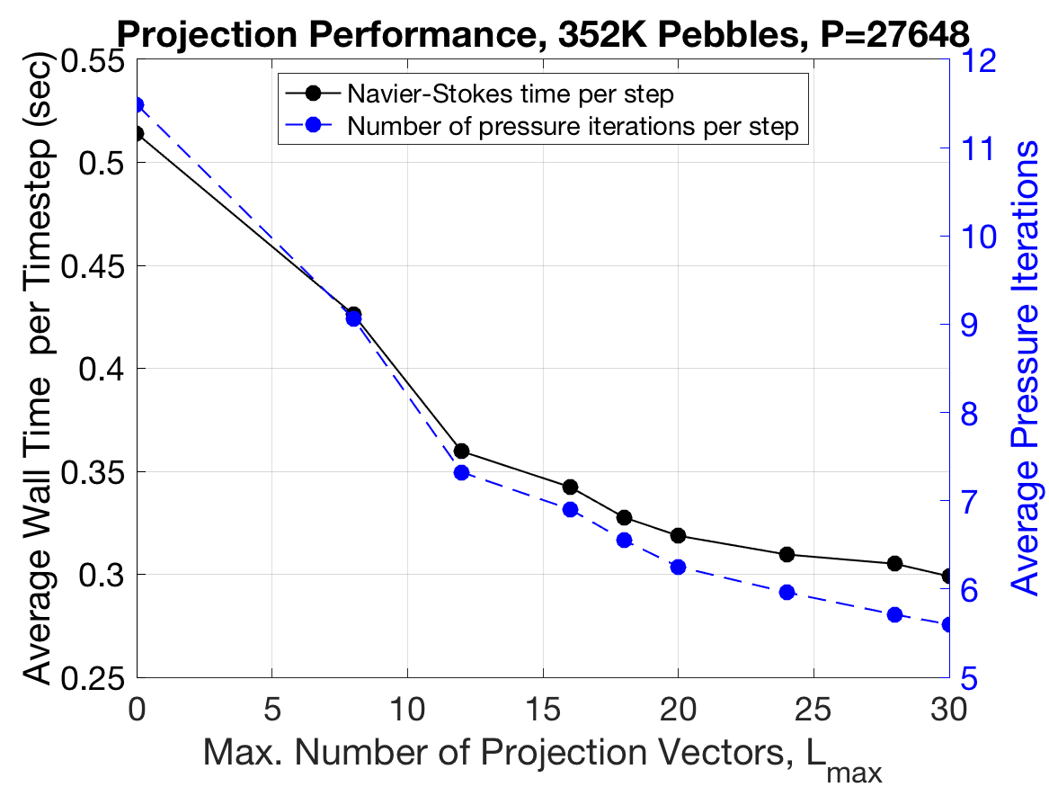
Figure 3: Average time per step and pressure iteration count as a function of projection-space dimension, $L_{\max}$.

NekRS Strong Scale: 352K pebbles, $E$=98M, $n$=50B
$N=8$, $N_{q}=13$, $\Delta t=$ 4.e-4, $L=8$, 1-Cheb-Jac:851
Node	GPU	$n/P$	$v_{i}$	$p_{i}$	$t_{\rm step}$	Eff
1536	9216	5.4M	3.6	17.3	.97	1.00
2304	13824	3.6M	3.6	18.0	.84	76.9
3072	18432	2.7M	3.6	16.6	.75	64.6
3840	23040	2.1M	3.6	19.6	.67	57.9
4608	27648	1.8M	3.6	17.5	.55	58.7
$N=8$, $N_{q}=13$, $\Delta t=$ 4.e-4, $L=8$, 1-Cheb-ASM:851
Node	GPU	$n/P$	$v_{i}$	$p_{i}$	$t_{\rm step}$	Eff
1536	9216	5.4M	3.6	11.6	.81	100
2304	13824	3.6M	3.6	12.3	.65	83.0
3072	18432	2.7M	3.6	12.3	.71	57.0
3840	23040	2.1M	3.6	13.5	.54	60.0
4608	27648	1.8M	3.6	12.8	.46	58.6
$N=8$, $N_{q}=11$, $\Delta t=$ 8.e-4, $L=30$, 2-Cheb-ASM:8641
Node	GPU	$n/P$	$v_{i}$	$p_{i}$	$t_{\rm step}$	Eff
1536	9216	5.4M	-	-	-	-
2304	13824	3.6M	5.7	7.2	.55	100
3072	18432	2.7M	5.7	7.2	.56	73.6
3840	23040	2.1M	5.7	7.2	.39	84.6
4608	27648	1.8M	5.7	7.2	.36	76.3

Table 6: NekRS Strong Scale using BDF2 with characteristic.

6 Conclusions

The simulations of full nuclear reactor cores described here are ushering in a new era for the thermal-fluids and coupled analysis of nuclear systems. The possibility of simulating such systems in all their size and complexity was unthinkable until recently. In fact, the simulations are already being used to benchmark and improve predictions obtained with traditional methods such as porous media models. This is important because models currently in use were not developed to predict well the change in resistance that occurs in the cross section due to the restructuring of the pebbles in the near wall region. This is a well known gap hindering the deployment of this class of reactors. Beyond pebble beds, the fact that such geometry can be addressed with such low time-to-solution will enable a broad range of optimizations and reductions in uncertainty in modeling that were until now not achievable in nuclear engineering. The impact will extend to all advanced nuclear reactor design with the ultimate result of improving their economic performance. This will in turn serve broadly the goal of reaching a carbon-free economy within the next few decades.

The study presented here demonstrates the continued importance of numerical algorithms in realizing HPC performance, with up to a four-fold reduction in solution times realized by careful choices among a viable set of options. This optimization was realized in relatively short time (a matter of days) by having a suite of solution algorithms and implementations available in NekRS—no single strategy is always a winner. For users, who often have a singular interest, being able to deliver best-in-class performance can make all the difference in productivity. In Nek5000 and NekRS, we support automated tuning of communication strategies that adapt to the network and underlying topology of the particular graph that is invoked at runtime. This approach has proven to make up to a factor of 4 difference, for example, in AMG implementations of the coarse-grid solver.

References

- Abdelfattah et al. (2020) Abdelfattah A, Barra V, Beams N, Bleile R, Brown J, Camier JS, Carson R, Chalmers N, Dobrev V, Dudouit Y, Fischer P, Karakus A, Kerkemeier S, Kolev T, Lan YH, Merzari E, Min M, Phillips M, Rathnayake T, Rieben R, Stitt T, Tomboulides A, Tomov S, Tomov V, Vargas A, Warburton T and Weiss K (2020) GPU algorithms for efficient exascale discretizations. Parallel Comput. submitted.
- Anderson et al. (2020) Anderson R, Andrej J, Barker A, Bramwell J, Camier JS, Dobrev JCV, Dudouit Y, Fisher A, Kolev T, Pazner W, Stowell M, Tomov V, Akkerman I, Dahm J, Medina D and Zampini S (2020) MFEM: A modular finite element library. Computers & Mathematics with Applications 10.1016/j.camwa.2020.06.009.
- Andreades et al. (2016) Andreades C, Cisneros AT, Choi JK, Chong AY, Fratoni M, Hong S, Huddar LR, Huff KD, Kendrick J, Krumwiede DL et al. (2016) Design summary of the mark-i pebble-bed, fluoride salt–cooled, high-temperature reactor commercial power plant. Nuclear Technology 195(3): 223–238.
- Arndt et al. (2017) Arndt D, Bangerth W, Davydov D, Heister T, Heltai L, Kronbichler M, Maier M, Pelteret J, Turcksin B and Wells D (2017) The deal.II library, version 8.5. J. Num. Math. 25(3): 137–145. URL www.dealii.org.
- Bajorek (2016) Bajorek SM (2016) A regulator’s perspective on the state of the art in nuclear thermal hydraulics. Nuclear Science and Engineering 184(3): 305–311.
- Chalmers et al. (2020) Chalmers N, Karakus A, Austin AP, Swirydowicz K and Warburton T (2020) libParanumal. URL github.com/paranumal/libparanumal.
- Cleveland and Greene (1986) Cleveland J and Greene SR (1986) Application of thermix-konvek code to accident analyses of modular pebble bed high temperature reactors (htrs). Technical report, Oak Ridge National Lab.
- Deville et al. (2002) Deville M, Fischer P and Mund E (2002) High-order methods for incompressible fluid flow. Cambridge: Cambridge University Press.
- Fischer et al. (2015) Fischer P, Heisey K and Min M (2015) Scaling limits for PDE-based simulation (invited). In: 22nd AIAA Computational Fluid Dynamics Conference, AIAA Aviation. AIAA 2015-3049.
- Fischer et al. (2020a) Fischer P, Kerkemeier S, Min M, Lan YH, Phillips M, Rathnayake T, Merzari E, Tomboulides A, Karakus A, Chalmers N and Warburton T (2020a) NekRS, a GPU-accelerated spectral element Navier–Stokes solver. Parallel Comput. submitted.
- Fischer et al. (2008) Fischer P, Lottes J and Kerkemeier S (2008) Nek5000: Open source spectral element CFD solver. http://nek5000.mcs.anl.gov and https://github.com/nek5000/nek5000 .
- Fischer et al. (2020b) Fischer P, Min M, Rathnayake T, Dutta S, Kolev T, Dobrev V, Camier JS, Kronbichler M, Warburton T, Swirydowicz K and Brown J (2020b) Scalability of high-performance PDE solvers. Int. J. of High Perf. Comp. Appl. 34(5): 562–586. URL https://doi.org/10.1177/1094342020915762.
- Fischer et al. (2017) Fischer P, Schmitt M and Tomboulides A (2017) Recent developments in spectral element simulations of moving-domain problems, volume 79. Fields Institute Communications, Springer, pp. 213–244.
- (14) Giraldo F (????) The nonhydrostatic unified model of the ocean (numo). https://frankgiraldo.wixsite.com/mysite/numo .
- Grötzbach and Wörner (1999) Grötzbach G and Wörner M (1999) Direct numerical and large eddy simulations in nuclear applications. International Journal of Heat and Fluid Flow 20(3): 222–240.
- Karakus et al. (2019) Karakus A, Chalmers N, Świrydowicz K and Warburton T (2019) A gpu accelerated discontinuous galerkin incompressible flow solver. J. Comp. Phys. 390: 380–404.
- Kreiss and Oliger (1972) Kreiss H and Oliger J (1972) Comparison of accurate methods for the integration of hyperbolic problems. Tellus 24: 199–215.
- Lottes and Fischer (2005) Lottes JW and Fischer PF (2005) Hybrid multigrid/Schwarz algorithms for the spectral element method. J. Sci. Comput. 24: 45–78.
- Maday et al. (1990) Maday Y, Patera A and Rønquist E (1990) An operator-integration-factor splitting method for time-dependent problems: Application to incompressible fluid flow. J. Sci. Comput. 5: 263–292.
- Malm et al. (2013) Malm J, Schlatter P, Fischer P and Henningson D (2013) Stabilization of the spectral-element method in convection dominated flows by recovery of skew symmetry. J. Sci. Comput. 57: 254–277.
- Markidis et al. (2015) Markidis S, Gong J, Schliephake M, Laure E, Hart A, Henty D, Heisey K and Fischer P (2015) Openacc acceleration of the Nek5000 spectral element code. Int. J. of High Perf. Comp. Appl. 1094342015576846.
- Medina et al. (2014) Medina DS, St-Cyr A and Warburton T (2014) OCCA: A unified approach to multi-threading languages. preprint arXiv:1403.0968 .
- Merzari et al. (2021a) Merzari E, Cheung FB, Bajorek SM and Hassan Y (2021a) 40th anniversary of the first international topical meeting on nuclear reactor thermal-hydraulics: Highlights of thermal-hydraulics research in the past four decades. Nuclear Engineering and Design 373: 110965.
- Merzari et al. (2020a) Merzari E, Fischer P, Min M, Kerkemeier S, Obabko A, Shaver D, Yuan H, Yu Y, Martinez J, Brockmeyer L et al. (2020a) Toward exascale: overview of large eddy simulations and direct numerical simulations of nuclear reactor flows with the spectral element method in nek5000. Nuclear Technology 206(9): 1308–1324.
- Merzari et al. (2020b) Merzari E, Obabko A, Fischer P and Aufiero M (2020b) Wall resolved large eddy simulation of reactor core flows with the spectral element method. Nuclear Engineering and Design 364: 110657.
- Merzari et al. (2017) Merzari E, Obabko A, Fischer P, Halford N, Walker J, Siegel A and Yu Y (2017) Large-scale large eddy simulation of nuclear reactor flows: Issues and perspectives. Nuclear Engineering and Design 312: 86–98.
- Merzari et al. (2021b) Merzari E, Yuan H, Min M, Shaver D, Rahaman R, Shriwise P, Romano P, Talamo A, Lan YH, Gaston D et al. (2021b) Cardinal: A lower length-scale multiphysics simulator for pebble-bed reactors. Nuclear Technology : 1–23.
- Moxey et al. (2020) Moxey D, Amici R and Kirby M (2020) Efficient matrix-free high-order finite element evaluation for simplicial elements. SIAM J. Sci. Comput. 42(3): C97–C123.
- Novak et al. (2021) Novak A, Carlsen R, Schunert S, Balestra P, Reger D, Slaybaugh R and Martineau R (2021) Pronghorn: A multidimensional coarse-mesh application for advanced reactor thermal hydraulics. Nuclear Technology : 1–32.
- Orszag (1980) Orszag S (1980) Spectral methods for problems in complex geometry. J. Comput. Phys. 37: 70–92.
- Otten et al. (2016) Otten M, Gong J, Mametjanov A, Vose A, Levesque J, Fischer P and Min M (2016) An MPI/OpenACC implementation of a high order electromagnetics solver with GPUDirect communication. Int. J. High Perf. Comput. Appl. .
- Patel et al. (2019) Patel S, Fischer P, Min M and Tomboulides A (2019) A characteristic-based, spectral element method for moving-domain problems. J. Sci. Comput. 79: 564–592.
- Patera (1984) Patera A (1984) A spectral element method for fluid dynamics : laminar flow in a channel expansion. J. Comput. Phys. 54: 468–488.
- Ravikumar et al. (2019) Ravikumar K, Appelhans D and Yeung P (2019) Acceleration of extreme scale pseudo-spectral simulations of turbulence using asynchronism. In: Proc. of the Int. Conf. for High Perf. Comp., Net., Storage and Analysis.
- Roelofs (2018) Roelofs F (2018) Thermal hydraulics aspects of liquid metal cooled nuclear reactors. Woodhead Publishing.
- Świrydowicz et al. (2019) Świrydowicz K, Chalmers N, Karakus A and Warburton T (2019) Acceleration of tensor-product operations for high-order finite element methods. Int. J. of High Performance Comput. App. 33(4): 735–757.
- Tufo and Fischer (2001) Tufo H and Fischer P (2001) Fast parallel direct solvers for coarse-grid problems. J. Parallel Distrib. Comput. 61: 151–177.
- Van Staden et al. (2018) Van Staden M, Neykov B and Mulder E (2018) Explicit modelling of randomly packed pebble bed using rans cfd modelling. Proc. HTR-2018 : 8–10.
- Yildiz et al. (2020) Yildiz MA, Botha G, Yuan H, Merzari E, Kurwitz RC and Hassan YA (2020) Direct numerical simulation of the flow through a randomly packed pebble bed. Journal of Fluids Engineering 142(4).