MATHMOD 2022
10th Vienna International Conference on Mathematical Modelling
July 27 - 29, 2022 – Vienna, Austria
Feedback control of social distancing for COVID-19 via elementary formulae

Abstract

Social distancing has been enacted in order to mitigate the spread of COVID-19. Like many authors, we adopt the classic epidemic SIR model, where the infection rate is the control variable. Its differential flatness property yields ele mentary closed-form formulae for open-loop social distancing scenarios, where, for instance, the increase of the number of uninfected people may be taken into account. Those formulae might therefore be useful to decision makers. A feedback loop stemming from model-free control leads to a remarkable robustness with respect to severe uncertainties and mismatches. Although an identification procedure is presented, a good knowledge of the recovery rate is not necessary for our control strategy.

I Introduction

In two years an abundant mathematically oriented literature has been devoted to the worldwide COVID-19 pandemic. Some of the corresponding calculations had even a significant political impact (see, e.g., [1, 61]). Note that in the field of mathematical epidemiology of infectious diseases the role of modeling human behavior became increasingly important in the last $15$ years. It gave birth to a novel research field named behavioral epidemiology of infectious diseases: see, e.g., [45, 83].

A novel control technique for improving the social distancing is presented here. This fundamental topic has already been tackled by many authors: see, e.g., [2, 3, 4, 7, 8, 9, 10, 12, 13, 16, 18, 19, 17, 21, 27, 28, 29, 32, 35, 39, 48, 51, 52, 53, 54, 57, 60, 59, 63, 70, 73, 79]. Most of those papers are based on the famous SIR (Susceptible-Infected-Recovered/Removed) model, which goes back to 1927 ([37]), or on some modifications of its compartments. This communication is also using the SIR model:

• When, like in several papers, the infection rate is the control variable, the SIR model is (differentially) flat ([26]). Remember that flatness-based control is one of the most popular model-based control setting, especially with respect to concrete applications: see, e.g., [6, 11, 20, 38, 41, 42, 50, 62, 64, 66, 67, 72, 69, 75, 76, 77, 88] for some recent publications. Note that flatness has already been utilized by [31] for studying COVID-19 but with other purposes.

• There are severe uncertainties: model mismatch, poorly known initial conditions, …We therefore close the loop around the reference trajectory via model-free control, or MFC, in the sense of [22, 23]. MFC, which is easy to implement, has already been illustrated in a number of practical situations. Some new contributions are listed here: [30, 33, 34, 40, 43, 46, 44, 49, 55, 56, 65, 68, 71, 74, 80, 81, 84, 85, 86, 89, 90, 91]. Let us single out here the excellent work by [78] on ventilators, which are related to COVID-19.

In order to be more specific consider a flat system with a single input $u$ and a single output $y$. Assume that $y$ is a flat output. Our strategy (see also [82, 24]) may be summarized as follows:

1. To any output reference trajectory $y^{\star}$ corresponds at once thanks to flatness an open-loop control $u^{\star}$.

2. Let $z$ be some measured output. Write $z^{\star}$ the corresponding reference trajectory. Set $u=u^{\star}+\Delta u$, where $\Delta u$ is the control of an ultra-local local model ([22]). Its output $\Delta z=z-z^{\star}$ is the tracking error. Closing the loop via an intelligent controller ([22]) permits to ensure local stability around $z^{\star}$ in spite of severe mismatches and disturbances.

Our paper is organized as follows:

• Section II shows that the SIR model, where the infection rate is the control variable, is flat and the population of recovered/removed individuals is a flat output; the recovery rate is identifiable in the sense of [25].

• Section III is devoted to a flatness-based control strategy, i.e., to a feedforward approach. Elementary closed-form of the control and state variables are easily derived. Various scenarios, where for instance the number of uninfected persons is increased, may thus be easily suggested to decision makers.

• Closing the loop via an intelligent proportional regulator, stemming from model-free control, is the subject of Section IV. Computer simulations confirm an excellent robustness with respect to severe uncertainties.

• A time-varying recovery rate is estimated in Section V via algebraic estimation methods ([25]). Techniques from Section IV show however good performances if this rate is wrongly assumed to be constant.

• Some suggestions for future investigations and someconcluding remarks may be found in Section VI.

II Modeling issues

II-A The SIR model

The SIR model (see, e.g., [87] for a nice introduction) reads:

$$\begin{cases}\dot{S}=-\beta IS\\ \dot{I}=\beta IS-\gamma I\\ \dot{R}=\gamma I\end{cases}$$ (1)

$S$, $I$ and $R$, which are non-negative quantities, correspond respectively to the fractions of susceptible, infected and recovered/removed individuals in the population. We may set therefore

$$S+I+R=1$$ (2)

$\beta$, $0<\underline{\beta}\leq\beta\leq\overline{\beta}$, which is here the control variable, and the parameter $\gamma>0$ are respectively the infection and recovery rates.

II-B Flatness

Equations (1)-(2) show that System (1) is flat and that $R$ is a flat output ([26]). The other system variables may be expressed as differential rational functions of $R$, i.e., as rational functions of $R$ and its derivatives up to some finite order:

$$I =\frac{\dot{R}}{\gamma}$$ (3)

$$S =1-R-\frac{\dot{R}}{\gamma}$$ (4)

$$\beta =-\frac{\dot{S}}{IS}=\frac{1}{S}\left(\frac{\dot{I}}{I}+\gamma\right)$$ (5)

Remark 1

If $\gamma$ is not constant, but a differentiable function of time, Equations (3)-(4)-(5) remain valid: System (1) is still flat and $R$ is still a flat output. Equation (5) shows however that $\dot{\gamma}$ is needed.

II-C An addendum on the SEIR model

The SEIR model (see, e.g., [14]) is a rather popular extension of the SIR model:

$$\begin{cases}\dot{S}=-\beta IS\\ \dot{E}=\beta IS-\alpha E\\ \dot{I}=\alpha E-\gamma I\\ \dot{R}=\gamma I\end{cases}$$ (6)

where $\alpha>0$ is an additional parameter. Equation (2) becomes

$$S+E+I+R=1.$$ (7)

Equations (6)-(7) show that the SEIR model is also flat and that $R$ is a flat output:

$$\left\{\begin{aligned} I&=\frac{\dot{R}}{\gamma}\\ E&=\frac{\dot{I}+\gamma I}{\alpha}=\frac{\ddot{R}+\gamma\dot{R}}{\gamma\alpha}\\ S&=1-R-I-E=1-R-\frac{\dot{R}}{\gamma}-\frac{\ddot{R}+\gamma\dot{R}}{\gamma\alpha}\\ \beta&=-\frac{\dot{S}}{IS}\end{aligned}\right.$$

II-D Identifiability of the recovery rate

Equation (5) yields

$$\gamma=\beta S-\frac{\dot{I}}{I}$$

$\gamma$ is a differential rational function .of $R$ and $\beta$: It is thus rationally identifiable ([25]).

Remark 2

The above equation does not work for an identifiability purpose if $\gamma$ is time-varying: $\dot{\gamma}$ is sitting on its right hand-side. If we assume that $I$ and $S$ are measured, Equation (4) yields

$$\gamma=\frac{\dot{I}-\beta IS}{I}$$ (8)

$\gamma$ is still rationally identifiable with respect to $I$, $S$, $\beta$. It will be useful in Section V.

III Flatness-based control

III-A Preparatory calculations

Set

$$\boxed{I_{\rm reference}(t)=I_{0}e^{-\lambda t}}$$

where $t\geq 0$, $0\leq I_{0}\leq 1$, and $\lambda\geq 0$ is some constant parameter. If we set $R(0)=0$, it yields

$$R_{\rm reference}(t)=\frac{\gamma I_{0}}{\lambda}(1-e^{-\lambda t})$$

$$S_{\rm reference}(t)=1-\frac{\gamma I_{0}}{\lambda}\left(1-e^{-\lambda t}\right)-I_{0}e^{-\lambda t}$$

and the open-loop control

$$\boxed{\beta_{\rm flat}(t)=\frac{\gamma-\lambda}{1-\frac{\gamma I_{0}}{\lambda}\left(1-e^{-\lambda t}\right)-I_{0}e^{-\lambda t}}}$$

Thus

$$\lim\limits_{t\to+\infty}\beta_{\rm flat}(t)=\frac{\lambda(\gamma-\lambda)}{\lambda-\gamma I_{0}}$$ (9)

The following inequalities are staightforward:

$$\gamma I_{0}<\lambda<\gamma$$ (10)

$\lambda<\gamma$ follows from $\beta>0$; $\gamma I_{0}<\lambda$ follows from

$$\lim\limits_{t\to+\infty}S(t)=1-\frac{\gamma I_{0}}{\lambda}=S(\infty)>0$$ (11)

Introduce the more or less precise quantity $\beta_{\rm accept}$, where $\underline{\beta}<\beta_{\rm accept}<\overline{\beta}$. It stands for the “harshest” social distancing protocols which are “acceptable” in the long run. Equation (9) yields therefore

$$\frac{\lambda(\gamma-\lambda)}{\lambda-\gamma I_{0}}=\beta_{\rm accept}$$

The positive root of the corresponding quadratic algebraic equation $\lambda^{2}+(\beta_{\rm accept}-\gamma)\lambda-\gamma I_{0}\beta_{\rm accept}=0$ is

$$\boxed{\lambda_{\rm accept}=\frac{{\gamma-\beta_{\rm accept}+\sqrt{\Delta_{\rm accept}}}}{2}}$$

where $\Delta_{\rm accept}=(\gamma-\beta_{\rm accept})^{2}+4\gamma I_{0}\beta_{\rm accept}\geq 0$. The fundamental inequality

$$\gamma I_{0}<\lambda_{\rm accept}<\gamma$$

follows from

$$\lim\limits_{\lambda\downarrow\gamma I_{0}}\frac{\lambda(\gamma-\lambda)}{\lambda-\gamma I_{0}}=+\infty,\quad\lim\limits_{\lambda\uparrow\gamma}\frac{\lambda(\gamma-\lambda)}{\lambda-\gamma I_{0}}=0$$

Equation (11) leads to the notation

$$S_{\rm accept}(\infty)=1-\frac{\gamma I_{0}}{\lambda_{\rm accept}}$$

The inequality

$$S(\infty)<S_{\rm accept}(\infty)\quad{\rm if}\quad\lambda<\lambda_{\rm accept}$$

demonstrates that the proportion of uninfected people decreases if the social distancing obligations are relaxed.

III-B Two computer experiments

Set $\gamma=0.1$, $\beta_{\rm accept}=0.22$. Figure 1 displays the open-loop evolutions of $\beta$, $I$, $S$ when $\lambda=\lambda_{\rm accept}$. Those behaviors are quite satisfactory.

IV Model-free control

IV-A Ultra-local model

Set $\Delta I(t)=I(t)-I_{\rm reference}(t)$, $\beta(t)=\beta_{\rm flat}(t)+\Delta\beta(t)$. In order to take into account the various uncertainties, introduce the ultra-local model ([22])

$$\frac{d}{dt}\Delta I=F+\mathfrak{a}\Delta\beta$$ (12)

• The function $F$, which is data-driven, subsumes the poorly known structures and disturbances.

• The parameter $\mathfrak{a}$, which does not need to be precisely determined, is chosen such that the three terms in Equation (12) are of the same magnitude.

• $F_{\rm est}=-\frac{6}{\tau^{3}}\int_{t-\tau}^{t}\left((t-2\sigma)\Delta I(\sigma)+\mathfrak{a}\sigma(\tau-\sigma)\Delta\beta(\sigma)\right)d\sigma$, where $\tau>0$ is “small”, gives a real-time estimate, which in practice is implemented via a digital filter.

IV-B Intelligent proportional controller

Introduce ([22]) the intelligent proportional controller, or iP,

$$\boxed{\Delta\beta=-\frac{F_{\rm est}+K_{P}\Delta I}{\mathfrak{a}}}$$ (13)

where $K_{P}$ is a tuning gain. Equations (12) and (13) yield

$$\frac{d}{dt}\Delta I+K_{P}\Delta I=F-F_{\rm est}$$

Set $K_{P}>0$. Then $\lim\limits_{t\to+\infty}\Delta I(t)\approx 0$ if the estimate $F_{\rm est}$ is “good,” i.e., if $F-F_{\rm est}$ is “small.” Local stability is ensured.

Remark 3

When compared to classic PIs and PIDs (see, e.g., [5]), the gain tuning of the iP is straightforward.

IV-C Computer experiments

The sampling time interval is $2$ hours. In Equations (12) and (13), $\mathfrak{a}=0.1$, $K_{P}=1$. Figure 2 displays excellent results in spite of errors on initial conditions and of the fuzzy character of any measurement of the social distancing. This fuzziness is expressed here by an additive corrupting white Gaussian noise $\mathcal{N}(0,5.10^{-3})$ on $\beta$.

V On the recovery rate $\gamma$

Assume now that $\gamma$ is a differentiable time function. Equation (8) yields the algebraic estimator

$$\gamma_{\rm est}=\frac{[\dot{I}]_{\rm est}-\beta IS}{I}$$ (14)

where $[\dot{I}]_{\rm est}$ is an estimate of $\dot{I}$ obtained along the lines developed by [47] and [58] for algebraic differentiators. Figure 3-c displays excellent results. The flatness-based computer experiments is achieved as in Section III-B, i.e., $\gamma=0.1$ is assumed to be constant. Lack of space prevents us from examining more realistic situations. Closing the loop via model-free control yields as demonstrated in Figures 3-a-b a satisfactory behavior. Is the exact knowledge of the recovery rate unimportant?

VI Conclusion

[15] questions the relevance and usefulness of such control-theoretic considerations for non-pharmaceutical mitigation policies against COVID-19. We certainly do not claim to set aside those objections in this preliminary short study. The combination however of flatness-based and model-free controls presents nevertheless some major advantages as demonstrated here and by [82] and [24].

An extra theoretical effort must be made in order to design control strategy as close as possible to the real epidemic control enacted by Public Health authorities. Summarizing, we consider this results proposed in this work as a theoretical ideal framework, to be filled with a more realistic picture: an implementable non-pharmaceutical control strategy. Preliminary results, which we recently obtained, indicate that the methodology here proposed is in the right direction (see [36]).

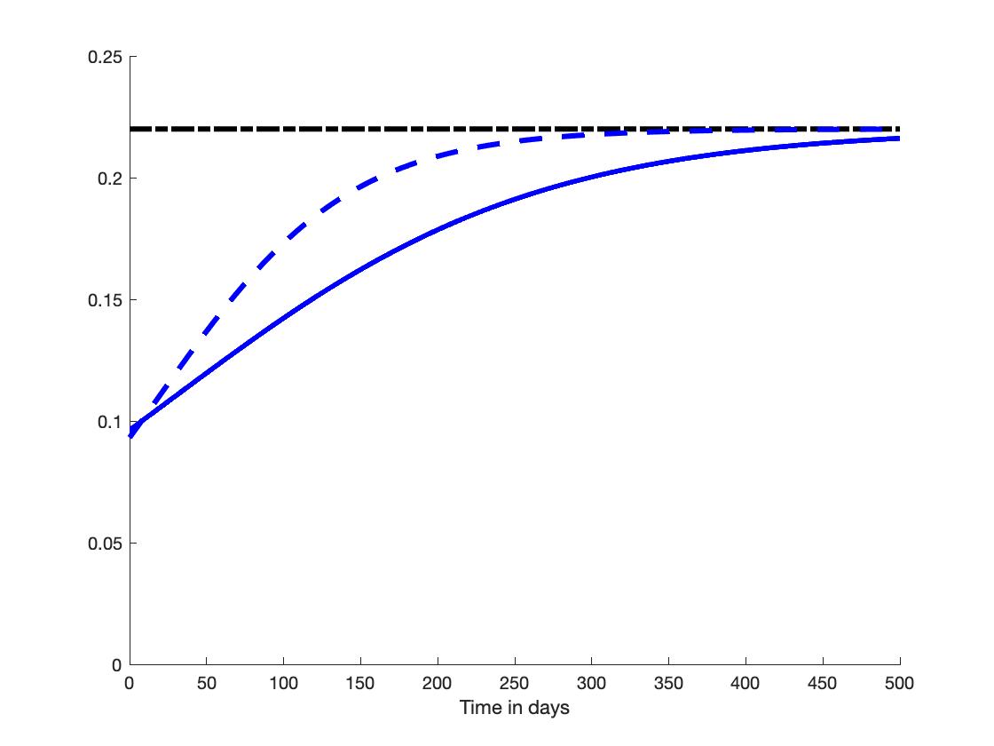
(a) $\beta$

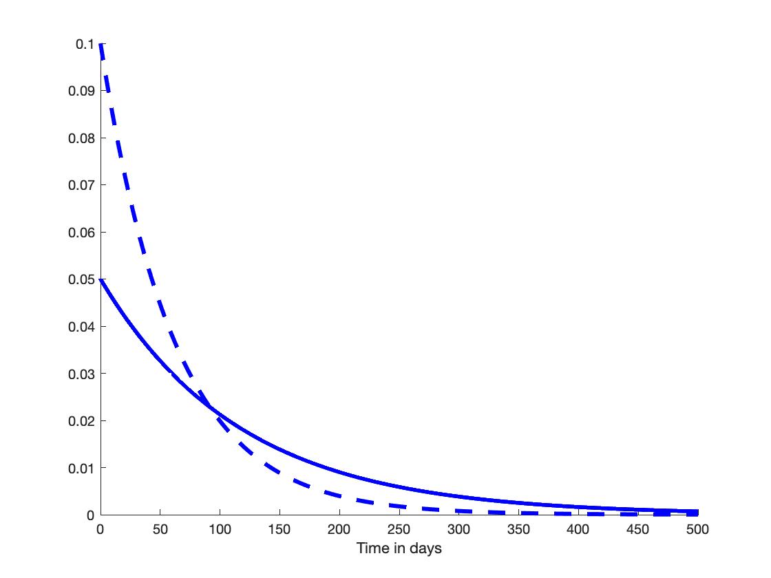
(b) $I$

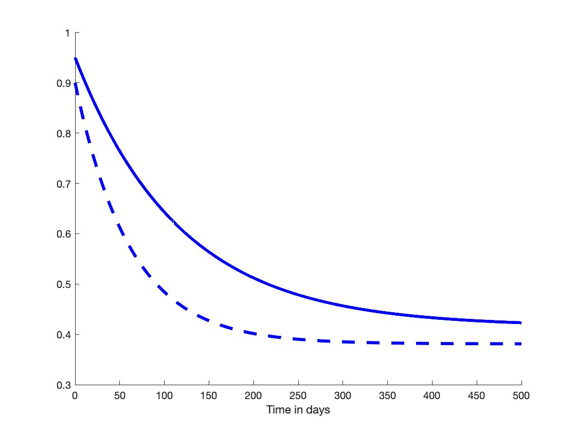
(c) $S$

Figure 1: Open loop control strategy. Trajectories corresponding to two distinct initial conditions for the infectius $I_{0}=0.05$ (single-dashed curves: -) and $I_{0}=0.1$ (double-dashed curves: - -). Left panel: plot of the transition rate $\beta(t)$; central panel: plot of the infectious fraction $I(t)$; right panel: plot of the fraction of susceptible subjects $S(t)$.

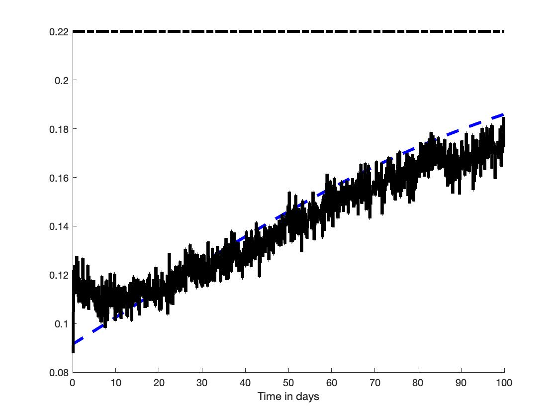
(a) $\beta$

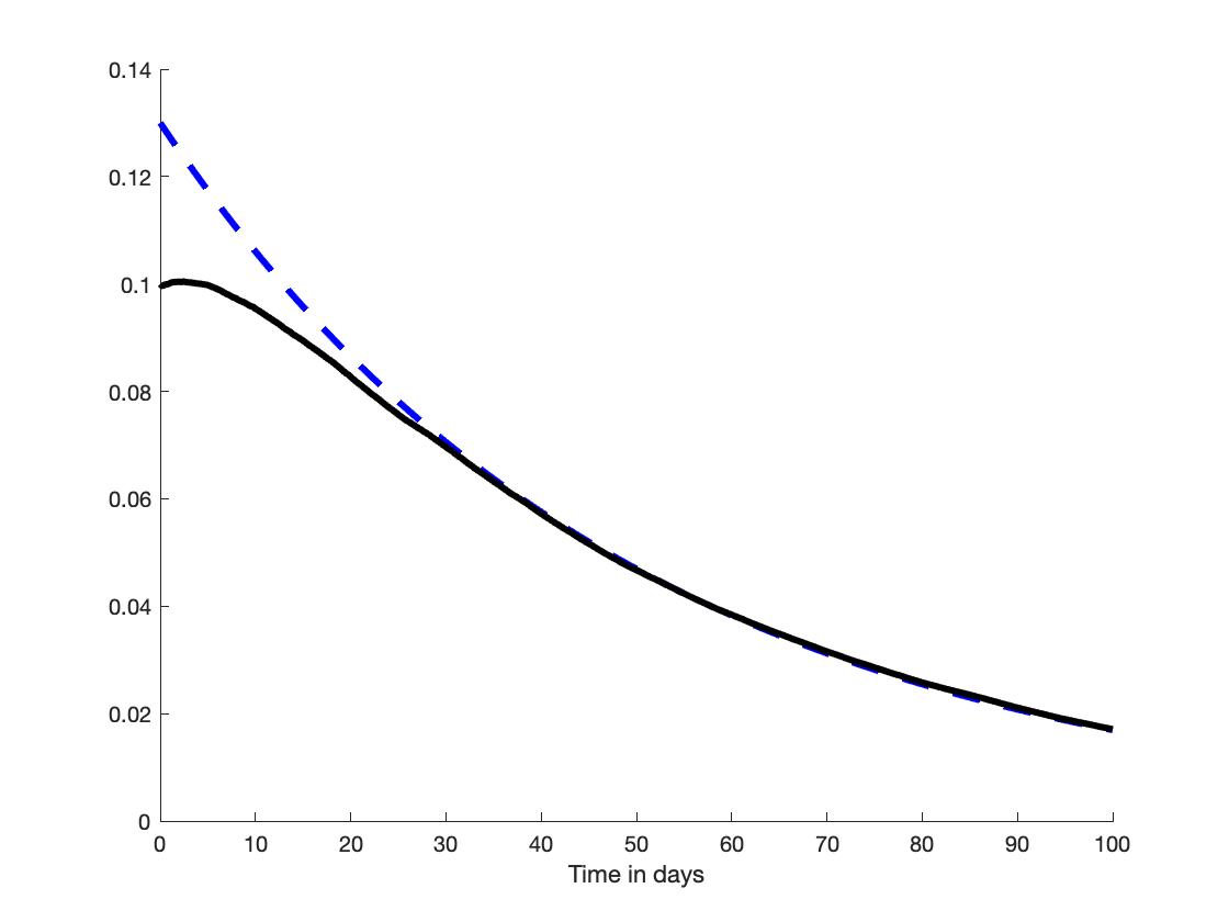
(b) $I$

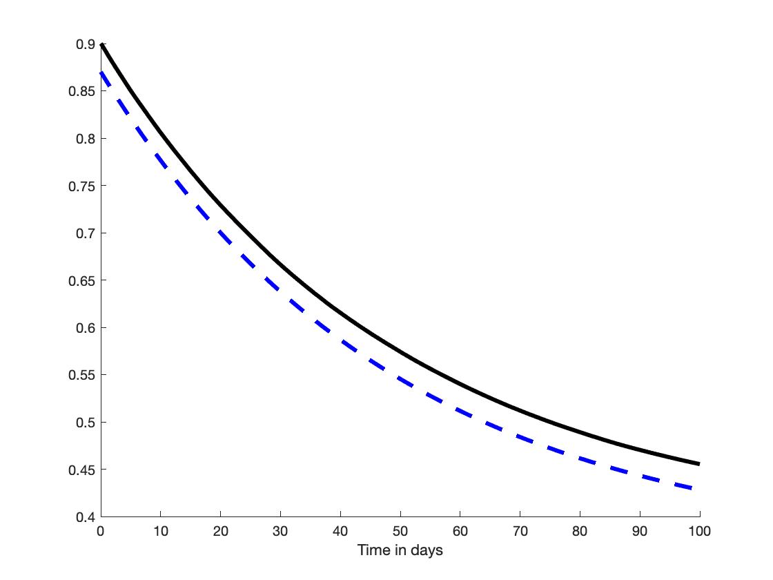
(c) $S$

Figure 2: Effect of both errors on initial conditions and of the fuzziness of measurements of social distancing. In all panels, dashed blue line represent the reference trajectories. Left panel: plot of the transition rate $\beta(t)$; central panel: plot of the infectious fraction $I(t)$; right panel: plot of the fraction of susceptible subjects $S(t)$.

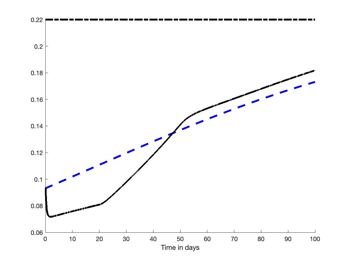
(a) $\beta$ – (blue - -): reference trajectory

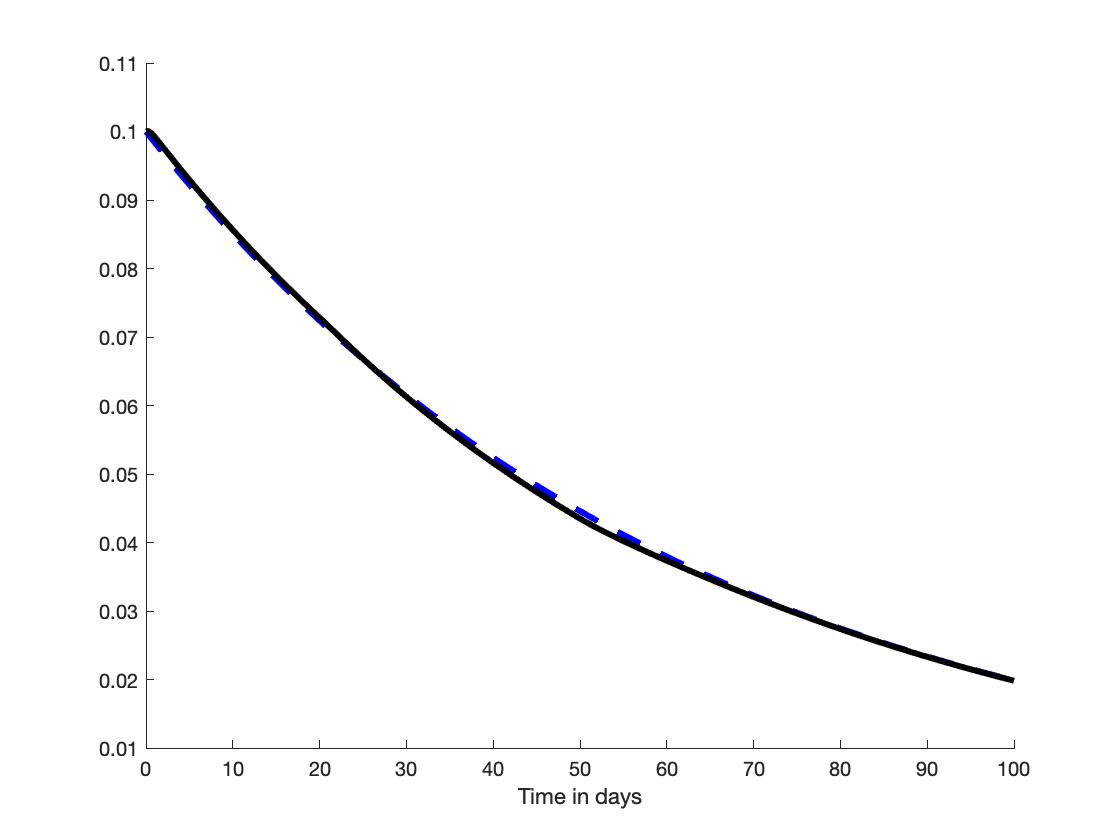
(b) $I$ – (blue - -): reference trajectory

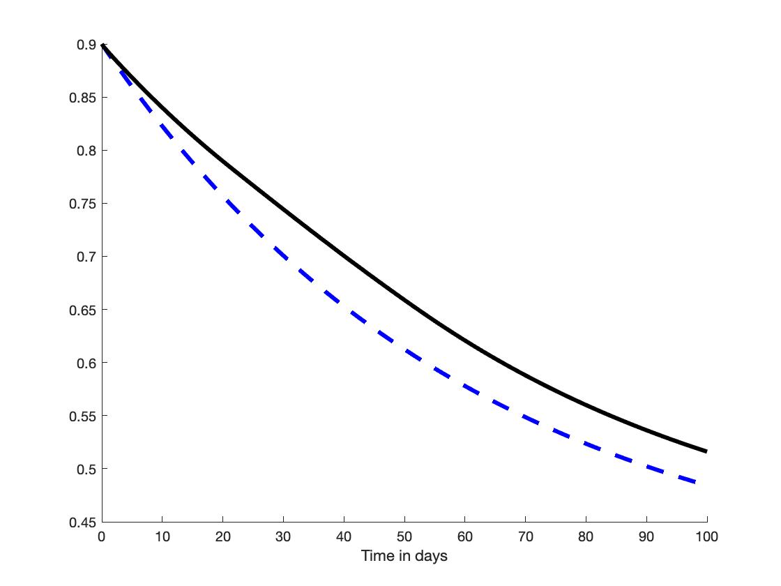
(c) $S$ – (blue - -): reference trajectory

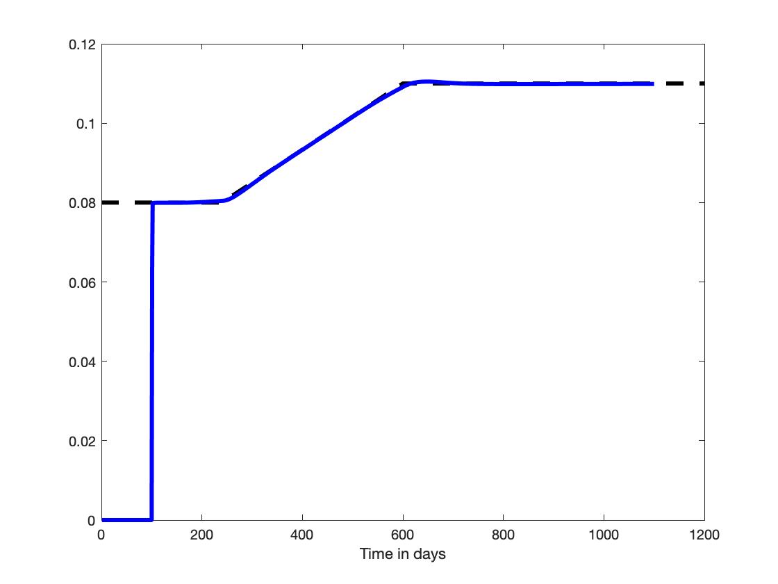
(d) $\gamma$ (- -) and $\gamma_{\rm est}$ (blue –)

Figure 3: Impact of the estimation of the time-varying recovery rate $\gamma$.

References

- [1] Adam D. (2020). Special report: the simulations driving the world’s response to COVID-19. Nature, 580, 316-318.
- [2] Al-Radhawi M.A., Sadeghi M., Sontag E.D. (2022). Long-term regulation of prolonged epidemic outbreaks in large populations via adaptive control: A singular perturbation approach. IEEE Contr. Syst. Lett., 6, 578-583.
- [3] Ames A.Z., Molnár T.G., Singletary A.W., Orosz G. (2020). Safety-critical control of active interventions for COVID-19 mitigation. IEEE Access, 8, 188454-188474.
- [4] Angulo M.T., Castaos F., Moreno-Morton R., Velasco-Hernández J.X., Moreno J.A. (2021). A simple criterion to design optimal non-pharmaceutical interventions for mitigating epidemic outbreaks. J. Roy. Soc. Interface, 18, 20200803.
- [5] Åström K.J., Murray R.M. (2008). Feedback Systems: An Introduction for Scientists and Engineers. Princeton University Press.
- [6] Beltran-Carbajal F., Tapia-Olvera R., Valderrabano-Gonzalez A., Yanez-Badillo H., Rosas-Caro J.C., Mayo-Maldonado J.C. (2021). Closed-loop online harmonic vibration estimation in DC electric motor systems. Appl. Math. Model., 94, 460-481.
- [7] Berger T. (2022). Feedback control of the COVID-19 pandemic with guaranteed non-exceeding ICU capacity. Syst. Contr. Lett., 160, 105111.
- [8] Bisiacco M., Pillonetto G. (2021). COVID-19 epidemic control using short-term lockdowns for collective gain. Ann. Rev. Contr., 52, 573-586.
- [9] Bliman P.-A., Duprez M. (2021). How best can finite-time social distancing reduce epidemic final size? J. Theoret. Biol., 511, 110557.
- [10] Bliman P.-A., Duprez M., Privat Y., Vauchelet N. (2021). Optimal immunity control and final size minimization by social distancing for the SIR epidemic model. J. Optim. Theory App., 189, 408-436.
- [11] Bonnabel S., Clayes X. (2020). The industrial control of tower cranes: An operator-in-the-loop approach. IEEE Contr. Syst. Magaz., 40, 27-39.
- [12] Bonnans J.F., Gianatti J. (2020). Optimal control techniques based on infection age for the study of the COVID-19 epidemic. Math. Model. Nat. Phenom., 15, 48.
- [13] Borri A., Palumbo P., Papa F., Possieri C. (2021). Optimal design of lock-down and reopening policies for early-stage epidemics through SIR-D models Annu. Rev. Contr. 51, 511-524.
- [14] Brauer F., Castillo-Chavez C. (2012). Mathematical Models in Population Biology and Epidemiology (2nd ed.). Springer.
- [15] Casella F. (2021). Can the COVID-19 epidemic be controlled on the basis of daily test reports? IEEE Contr. Syst. Lett., 5, 1079-1084.
- [16] Charpentier A., Elie R., Laurière‘M., Tran V.C. (2020). COVID-19 pandemic control: balancing detection policy and lockdown intervention ICU sustainability. Math. Model. Nat. Phenom., 15, 57.
- [17] Dias S., Queiroz K., Araujo A. (2022). Controlling epidemic diseases based only on social distancing level. J. Contr. Autom. Electr. Syst., 33, 8-22.
- [18] Di Lauro F., Kiss I.Z., Della Santina C. (2021a). Optimal timing of one-shot interventions for epidemic control. PLoS Comput. Biol., 17, e1008763.
- [19] Di Lauro F., Kiss I.Z., Della Santina C. (2021b). Covid-19 and flattening the curve: A feedback control perspective. IEEE Contr. Syst. Lett., 5, 1435-1440.
- [20] Diwold J., Kolar B., Markus Schöberl M. (2022). Discrete-time flatness-based control of a gantry crane. Contr. Engin. Pract., 119, 104980.
- [21] Efimov D., Ushirobira R. (2021). On an interval prediction of COVID-19 development based on a SEIR epidemic model. Ann. Rev. Contr., 51, 477-487.
- [22] Fliess M., Join C. (2013). Model-free control. Int. J. Contr., 86, 2228-2252.
-
[23]
Fliess M., Join C. (2021).
An alternative to proportional-integral and proportional-integral-derivative regulators: Intelligent proportional-derivative regulators.
Int. J. Robust Nonlin. Contr.
https://doi.org/10.1002/rnc.5657 - [24] Fliess M., Join C., Moussa K., Djouadi S.M., Alsager M.W. (2021). Toward simple in silico experiments for drugs administration in some cancer treatments. IFAC PapersOnLine, 54-15, 245-250.
- [25] Fliess M., Join C., Sira-Ramìrez H. (2008). Non-linear estimation is easy. Int. J. Model. Identif. Contr., 4, 12-27.
- [26] Fliess M., Lévine J., Martin P., Rouchon P. (1995). Flatness and defect of non-linear systems: introductory theory and examples. Int. J. Contr., 61, 1327-1361.
- [27] Gevertz J.L., Greene J.M., Sanchez-Tapia C.H., Sontag E.D. (2021). A novel COVID-19 epidemiological model with explicit susceptible and asymptomatic isolation compartments reveals unexpected consequences of timing social distancing. J. Theoret. Biol., 510, 110539.
- [28] Godara P., Herminghaus S., Heidemann K.M. (2021). A control theory approach to optimal pandemic mitigation. PLoS ONE, 16, e0247445.
-
[29]
Greene J.M., Sontag E.D. (2021).
Minimizing the infected peak utilizing a single lockdown: a technical result regarding equal peak.
MedRxiv.
https://doi.org/10.1101/2021.06.26.21259589 - [30] Gu J., Li H., Zhang H., Pan C., Luan Z. (2021). Cascaded model-free predictive control for single-phase boost power factor correction converters. Int. J. Robust Nonlinear Contr., 31, 5016-5032.
- [31] Hametner C., Kozek M., Böhler L., Wasserburger A., Peng Du Z., Kölbl R., Bergmann M., Bachleitner-Hofmann T., Jakubek S. (2021). Estimation of exogenous drivers to predict COVID-19 pandemic using a method from nonlinear control theory. Nonlin. Dyn., 106, 1111-1125.
- [32] Ianni A., Rossi N. (2021). SIR-PID: A proportional-integral-derivative controller for COVID-19 outbreak containment. Physics, 3, 459-472.
- [33] Ismail A., Noura H., Harmouch F., Harb Z. (2021). Design and control of a neonatal incubator using model-free control. 29th Medit. Conf. Contr. Automat., Puglia.
- [34] Jin N., Chen M., Guo L., Li Y., Chen Y. (2021). Double-vector model-free predictive control method for voltage source inverter with visualization analysis. IEEE Trans. Indust. Electron. doi: 10.1109/TIE.2021.3128905
- [35] Jing M., Yew Ng K., Mac Namee B., Biglarbeigi P., Brisk R., Bond R., Finlay D., McLaughlin J. (2021). COVID-19 modelling by time-varying transmission rate associated with mobility trend of driving via Apple Maps. J. Biomed. Informat., 122, 103905.
- [36] Join C., d’Onofrio A., Fliess M. (2022). Toward realistic social distancing policies via advanced feedback control. Submitted.
- [37] Kermack W.O., McKendrick A.G. (1927). A contribution to the mathematical theory of epidemics. Proc. Royal Soc. London Ser. A, 115, 700-721.
- [38] Kogler H., Ladner K., Ladner P. (2022). Flatness-based control of a closed-circuit hydraulic press. In: Irschik H., Krommer M., Matveenko V.P., Belyaev A.K. (Eds) Dynamics and Control of Advanced Structures and Machines. Advanced Structured Materials, pp. 111-121. Springer.
- [39] Köhler J., Schwenkel L., Koch A., Berberich J., Pauli P., Allgöwer F. (2021). Robust and optimal predictive control of the COVID-19 outbreak. Ann. Rev. Contr., 51, 525-539.
- [40] Kuruganti T., Olama M., Dong J., Xue Y., Winstead C., Nutaro J., Djouadi S., Bai L., Augenbroe G., Hill J. (2021). Dynamic Building Load Control to Facilitate High Penetration of Solar Photovoltaic Generation. Tech. Rep. ORNL/TM-2021/2112, Oak Ridge National Lab.
- [41] Li X., Wang Y., Guo X., Cui X., Zhang S., Li Y.(2021). An improved model-free current predictive control method for SPMSM drives. IEEE Access, DOI: 10.1109/ACCESS.2021.3115782
- [42] Lorenz-Meyer M.N.L., Menzel R., Dadzis K., Nikiforova A., Riemann H. (2020). Lumped parameter model for silicon crystal growth from granulate crucible. Cryst. Res. Techno., 55, 2000044.
- [43] Lv M., Gao S., Wei Y., Zhang D., Qi H., Wei Y. (2022). Model-free parallel predictive torque control based on ultra-local model of permanent magnet synchronous machine. Actuators, 11, 31.
- [44] Mao J., Li H., Yang L., Zhang H., Liu L., Wang X., Tao J. (2021). Non-cascaded model-free predictive speed control of SMPMSM drive system. IEEE Trans. Energ. Convers., doi: 10.1109/TEC.2021.3090427
- [45] Manfredi P., d’Onofrio A. (Eds) (2013). Modeling the Interplay Between Human Behavior and the Spread of Infectious Diseases. Springer.
- [46] Manzoni E., Rampazzo M. (2021). Automatic regulation of anesthesia via ultra-local model control via ultra-local model control. IFAC PapersOnLine, 54-15, 49-54.
- [47] Mboup M., Join C., Fliess M. (2009). Numerical differentiation with annihilators in noisy environment. Numer. Algor., 50, 439-467.
- [48] McQuade S.T., Weightman R., Merrill N.J., Yadav A., Trélat E., Allred S.R., Piccoli B. (2021). Control of COVID-19 outbreak using an extended SEIR model. Math. Model. Meth. Appl. Sci., 31, 2399-2424.
- [49] Michel L., Silva C.J., Torres D.F.M. (2022). Model-free based control of a HIV/AIDS prevention model. Math. Biosci. Engin., 19, 759-774.
- [50] Miunske T. (2020). Ein szenarienadaptiver Bewegungsalgorithmus für die Längsbewegung eines vollbeweglichen Fahrsimulators. Springer.
- [51] Morato M.M., Bastos S.B., Cajueiro D.O., Normey-Rico J.E. (2020a). An optimal predictive control strategy for COVID-19 (SARS-CoV-2) social distancing policies in Brazil. Annual Rev. Contr., 50, 417-431.
-
[52]
Morato M.M., Pataro I.M.L., Americano da Costa M.V., Normey-Rico J.E. (2020b).
A parametrized nonlinear predictive control strategy for relaxing COVID-19 social distancing measures in Brazil.
ISA Trans.,
https://doi.org/10.1016/j.isatra.2020.12.012 - [53] Morgan A.L.K., Woolhouse M.E.J., Medley G.F., van Bunnik B.A.D. (2021). Optimizing time-limited non-pharmaceutical interventions for COVID-19 outbreak control. Phil. Trans. Roy. Soc. B, 376, 20200282.
- [54] Morris D.H., Rossine F.W., Plotkin J.B., Levin S.A. (2021). Optimal, near-optimal, and robust epidemic control. Communic. Phys., 4, 78.
- [55] Mousavi M.S., Davari S.A., Nekoukar V., Garcia C., Rodriguez J. (2021). Model-free finite set predictive voltage control of induction motor. 12th Power Electron. Drive Syst. Techno. Conf., Tabriz.
- [56] das Neves P.G., Augusto Angélico B.A. (2021). Model-free control of mechatronic systems based on algebraic estimation. Asian J. Contr., https://doi.org/10.1002/asjc.2596
- [57] O’Sullivan D., Gahegan M., Exeter D.J., Adams B. (2020). Spatially explicit models for exploring COVID-19 lockdown strategies. Trans. GIS, 24, 967-1000.
- [58] Othmane A., Rudolph J., Mounier H. (2021). Systematic comparison of numerical differentiators and an application to model-free control. Europ. J. Contr., 62, 113-119.
- [59] Pillonetto G., Bisiacco M., Palù G., Cobelli C. (2021). Tracking the time course of reproduction number and lockdown’s effect on human behaviour during SARS-CoV-2 epidemic: nonparametric estimation. Sci. Rep., 11, 9772.
- [60] Péni T., Csutak B., Szederkényi G., Röst G. (2020). Nonlinear model predictive control with logic constraints for COVID-19 management. Nonlin. Dyn., 102, 1965-1986.
- [61] Quintana I.O., Rosenstock S., Klein C. (2021). The coordination dilemma for epidemiological modelers. Biol. Philo., 36, 54.
- [62] Richter H., Warner H. (2021). Motion optimization for musculoskeletal dynamics: A flatness-based polynomial approach. IEEE Trans. Automat. Contr., DOI: 10.1109/TAC.2020.3029318
- [63] Sadeghi M., Greene J.M., Sontag E.D. (2021). Universal features of epidemic models under social distancing guidelines. Annual Rev. Contr., 51, 426-440.
- [64] Sahoo S.R., Chiddarwar S.S. (2020). Flatness-based control scheme for hardware-in-the-loop simulations of omnidirectional mobile robot. Simul., 96, 169-183.
- [65] Sancak C., Yamac F., Itik, M., Alici G. (2021). Force control of electro-active polymer actuators using model-free intelligent control. J. Intel. Mater. Syst. Struct., https://doi.org/10.1177/1045389X20986992
- [66] Sanchez J.C., Gavilan F., Vazqueza R., Louembet C. (2020). A flatness-based predictive controller for six-degrees of freedom spacecraft rendezvous. Acta Astronaut., 167, 391-403.
- [67] Schörghuber C., Gölles M., Reichhartinger M., Horn M. (2020). Control of biomass grate boilers using internal model control. Contr. Eng. Pract., 96, 104274.
- [68] Sehili L., Boukhezzar B. (2022). Ultra-local model design based on real-time algebraic and derivative estimators for position control of a DC motor. J. Contr. Autom. Electr. Syst., https://doi.org/10.1007/s40313-021-00881-z
- [69] Sekiguchi K., Eikyu W., Nonaka K. (2021). Feedback control for a drone with a suspended load via hierarchical linearization. J. Robot. Mechatron., 33, 274-282.
- [70] Sontag E.D. (2021).. An explicit formula for minimizing the infected peak in an SIR epidemic model when using a fixed number of complete lockdowns. Int. J. Robust Nonlin. Contr., https://doi.org/10.1002/rnc.5701
- [71] Srour A., Noura H., Theilliol (2021). Passive fault-tolerant control of a fixed-wing UAV based on model-free control. 5th Conf. Contr. Fault Toler. Syst. (SysTol), Saint-Raphaël.
- [72] Steckler P.-B., Gauthier J.-Y., Lin-Shi X., Wallart (2021). Differential flatness-based, full-order nonlinear control of a modular multilevel converter (MMC). IEEE Trans. Contr. Syst. Techno., DOI: 10.1109/TCST.2021.3067887
- [73] Stella L., Pinel Martínez A., Bauso D., Colaneri P. (2022). The role of asymptomatic infections in the COVID-19 epidemic via complex networks and stability analysis. SIAM J. Contr. Optim., S119-S144.
- [74] Sun J., Wang J., Yang P., Guo S. (2021). Model-free prescribed performance fixed-time control for wearable exoskeletons. Appl. Math. Model., 90, 61-77.
- [75] Tal E.A., Karaman S. (2021). Global trajectory-tracking control for a tailsitter flying wing in agile uncoordinated flight. AIAA Aviat. Forum.
- [76] Thounthong P., Mungporn P., Guilbert D., Takorabet N., Pierfedericie S., Nahid-Mobarakehf B., Hug Y., Bizonh N., Huangfui Y., Kumamj P. (2021). Design and control of multiphase interleaved boost converters-based on differential flatness theory for PEM fuel cell multi-stack applications. Elect. Power Ener. Syst, 124, 106346.
- [77] Tognon M., Franchi A. (2021). Theory and Applications for Control of Aerial Robots in Physical Interaction Through Tethers. Springer.
- [78] Truong C.T., Huynh K.H., Duong V.T., Nguyen H.H., Pham L.A., Nguyen T.T. (2021). Model-free volume and pressure cycled control of automatic bag valve mask ventilator. AIMS Bioengin., 8, 192-207.
- [79] Tsay C., Lejarza F., Stadtherr M.A., Baldea M. (2020). Modeling, state estimation, and optimal control for the US COVID-19 outbreak. Scientif. Rep., 10, 10711.
- [80] Xu L., Chen G., Li Q. (2020). Ultra-local model-free predictive current control based on nonlinear disturbance compensation for permanent magnet synchronous motor. IEEE Access, 8, 127690-127699.
- [81] Xu L., Chen G., Li Q. (2021). Cascaded speed and current model of PMSM with ultra-local model-free predictive control. Int. J. Robust Nonlinear Contr.. https://doi.org/10.1049/elp2.12108
- [82] Villagra, J., Herrero-Pérez, D. (2012). A comparison of control techniques for robust docking maneuvers of an AGV. IEEE Trans. Contr. Syst. Techno., 20, 1116-1123.
- [83] Wang Z., Bauch C.T., Bhattacharyya S., d’Onofrio A., Manfredi P., Perc M., Perra N., Salathè M., Zhao D. (2013). Statistical physics of vaccination. Phys. Rep., 664, 1-113.
- [84] Wang Z., Cosio A., Wang J. (2022). Implementation resource allocation for collision-avoidance assistance systems considering driver capabilities. IEEE Trans. Intel. Transport. Syst.
- [85] Wang Y., Li H., Liu R., Yang L., Wang X. (2020a). Modulated model-free predictive control with minimum switching losses for PMSM drive system. IEEE Access, 8, 20942-20953.
- [86] Wang Z., Wang J. (2020b). Ultra-local model predictive control: A model-free approach and its application on automated vehicle trajectory tracking. Contr. Eng. Pract., 101, 104482.
- [87] Weiss H. (2013). The SIR model and the foundations of public health. Materials matemàtics, https://ddd.uab.cat/record/108432
- [88] Zauner M., Mandl P., König O., Hametner C., Jakubek S. (2021). Stability analysis of a flatness-based controller driving a battery emulator with constant power load. at-Automatisierungstech, 69,142-154.
- [89] Zhang Y., Jiang T., Jiao J. (2020). Model-free predictive current control of a DFIG using an ultra-local model for grid synchronization and power regulation. IEEE Trans. Energ. Conv., 35, 2269-2280.
- [90] Zhang Y., Wang X., Yang H., Zhang B., Rodriguez J. (2021). Robust predictive current control of induction motors based on linear extended state observer. Chinese J. Elec. Engin., 7, 94-105.
- [91] Zhou Z., Wang Z., Wang J. (2021). Real-time adaptive threshold adjustment for lane detection application under different lighting conditions using model-free control. IFAC PapersOnLine, 54-20, 147-152.
- [92]