On the Maximum Achievable Sum-rate of the RIS-aided MIMO Broadcast Channel

Abstract

Reconfigurable intelligent surfaces (RISs) represent a new technology that can shape the radio wave propagation and thus offers a great variety of possible performance and implementation gains. Motivated by this, we investigate the achievable sum-rate optimization in a broadcast channel (BC) in the presence of reconfigurable intelligent surfaces. We solve this problem by exploiting the well-known duality between the Gaussian multiple-input multiple-output (MIMO) BC and the multiple-access channel (MAC), and we correspondingly derive three algorithms which optimize the users’ covariance matrices and the RIS phase shifts in the dual MAC. The users’ covariance matrices are optimized by a dual decomposition method with block coordinate maximization (BCM), or by a gradient-based method. The RIS phase shifts are either optimized sequentially by using a closed-form expression, or are computed in parallel by using a gradient-based method. We present a computational complexity analysis for the proposed algorithms. Simulation results show that the proposed algorithms tend to converge to the same achievable sum-rate overall, but may produce different sum-rate performance for some specific situations, due to the non-convexity of the considered problem. Also, the gradient-based optimization methods are generally more time efficient. In addition, we demonstrate that the proposed algorithms can provide a significant gain in the RIS-assisted BC assisted by multiple RISs and that the gain depends on the placement of the RISs.

I Introduction

The need to satisfy constantly increasing data rate demands in wireless communication networks motivates the development of new technology solutions such as RISs. An RIS is a metasurface that consists of a large number of small, low-cost, and passive elements, as well as low-power electronic circuits such as diodes or varactors. Since each of these elements can reflect the incident signal with an adjustable phase shift, an RIS can effectively shape the propagation of the impinging waves [2, 3]. Therefore, the introduction of RISs offers a wide variety of possible implementation gains and potentially presents a new milestone in wireless communications.

In order to fully exploit the gains that arise from the use of RISs, we need to obtain a deep understanding of different aspects of RIS-assisted wireless communication systems. Probably the most important aspect is concerned with the optimal design of the RIS phase shifts, so that the incoming radio wave is altered in a way that maximizes the aforementioned gains. In this regard, the development of algorithms for optimizing the achievable rate is of particular interest for RIS-aided communications. A significant body of research work in this area concentrates on optimizing the achievable rate for point-to-point MIMO communications. The algorithms proposed in [4] and [5] provide efficient methods for optimizing the transmit covariance matrix; however, these works do not deal with multi-user MIMO. The optimization of the achievable rate for a single-stream MIMO system in an indoor millimeter-wave (mmWave) environment with a blocked direct link was analyzed in [6]. The optimization schemes proposed in [6] provide a near-optimal achievable rate and require a low computational and hardware complexity. As far as discrete signaling is concerned, the authors of [7] have demonstrated that the achievable rate in RIS-aided systems can be efficiently maximized by using the cutoff rate as a more tractable optimization metric. The spectral efficiency enhancement arising from the addition of a small number of active elements to the RIS was considered in [8].

The optimization of the sum-rate in multi-user RIS-aided systems has received increasing research attention as well. In [9], the authors introduced an optimization method that increases the receive signal-to-noise ratio (SNR) and consequently enhances the achievable rate in multiple-input single-output (MISO) systems. The proposed solution is based on the AO method, which adjusts the transmit beamformer and the RIS phase shifts in an alternating fashion. The AO technique has also been successfully utilized to increase the data rate for secure communications in environments with multiple RISs and single-antenna users [10]. In [11], the authors employed a gradient-based algorithm to enhance the receive signal-to-interference-plus-noise ratio (SINR), and hence the achievable rate, for single-antenna users that do not have a direct link with the base station (BS). The sum-rate optimization for multi-user downlink communications based on a deep reinforcement learning based algorithm was introduced in [12]. In [13], the authors derived an expression for the ergodic achievable rate that depends on the statistical channel state information (CSI). As a result, configuring the RIS in [13] only requires knowledge of the CSI statistics, which are assumed to change slowly. An analytical framework for analyzing and optimizing the uplink and downlink transmissions of RIS-assisted cell-free massive MIMO systems when spatial correlation is present among the elements of the RIS was introduced in [14]. In [15], the achievable sum-rate in a multi-cell non-orthogonal multiple access (NOMA) network was optimized with respect to different network resources such as user association, subchannel assignment, power allocation, phase shift design, and decoding order.

The aforementioned papers consider single-antenna user devices in multi-user RIS-aided communications. On the other hand, a relatively small number of papers study the use of multi-antenna user devices in multi-user RIS-aided communications. This is due to the high intractability of the resulting optimization problems. The use of an RIS in multi-cell MIMO systems was investigated in [16] with the aim of improving the weighted sum-rate, in particular for application to the downlink transmission of cell-edge users. Because of the inherent non-convexity of the optimization problem, it was first reformulated and then solved by using the block coordinate descent (BCD) algorithm, according to which the precoding matrices and the RIS phase shifts are alternately optimized. Replacing some BSs with RISs in a multi-user MIMO cell-free network with multi-carrier transmission was studied in [17]. For the considered system, the authors proposed an AO-based optimization method, which takes the specific features of multi-carrier transmission into account for maximizing the weighted sum-rate. The achievable rate optimization in cell-free networks with multiple BSs and RISs was studied in [18]. Therein, optimization algorithms for the BS transmit beamforming matrices and the RIS phase shifts were separately derived, and later combined in an alternating manner. An AO-based algorithm for maximizing a closed-form expression for the asymptotic ergodic sum-rate in an RIS-aided MIMO MAC without a direct link between users and the BS was presented in [19]. An AO algorithm for maximizing the global energy efficiency for uplink transmission when only partial CSI is known was proposed in [20]. More precisely, statistical CSI was used for resource allocation in the considered multi-user MIMO uplink networks, under the assumption that all the signals are transmitted to the BS only via the RIS. The achievable sum-rate optimization based on a priori statistical knowledge of the users’ locations for computing the phase shifts of the RIS elements was introduced in [21]. In [22], the authors introduced an algorithm for optimizing the RISs and the hybrid-structured precoders/combiners, in addition to a corresponding channel estimation method, for application to an RIS-aided network operating in the Terahertz frequency band.

All of the aforementioned papers assume, however, linear transmit beamforming/precoding, which does not necessarily achieve the capacity of the BC. On the other hand, dirty paper coding (DPC) is an efficient technique for achieving the channel capacity in the MIMO BC. In [23], it was shown that implementing DPC in a BC achieves the maximum sum-rate. However, the analysis in [23] was constrained to a broadcast communication system with only two single-antenna user terminals. The work in [23] was extended to the case with multiple users equipped with multiple antennas in [24]. A duality between the capacity region of a MIMO system with DPC in a BC and the capacity region of the MIMO MAC was established in [25]. Accordingly, the capacity region of a MIMO BC with DPC was proved to be the same as the capacity region of the dual MIMO MAC, under the assumption that the transmitters have the same sum power constraint as the MIMO BC. Utilizing this duality, the authors proposed simple and fast iterative algorithms that provide the sum capacity achieving strategy for the dual MAC, which can easily be converted to the equivalent optimal strategies for the BC [26]. An application of the BC-MAC duality to a multi-user MISO system was studied in [27]. More precisely, the duality between a BC with zero-forcing (ZF)-DPC and a MAC with ZF-based successive interference cancellation (SIC) was used to design the transmit beamformer. To the best of the authors’ knowledge, the only paper that exploits the BC-MAC duality for studying the capacity/achievable rate regions for the MAC and for the BC in RIS-aided communications is [28]. However, the analysis presented in [28] was limited to single-antenna user terminals and a single-antenna BS, and can not be directly extended to multi-antenna devices.

The contributions of this paper are listed as follows:

• We exploit the Gaussian MIMO BC-MAC duality to maximize the achievable sum-rate of a multi-user MIMO system equipped with RISs communicating over a BC, and formulate an optimization problem of the users’ covariance matrices and the phase shifts of the RIS elements.

• Due to the non-convexity of the optimization problem and the possibility that a local optimization method may be trapped in a bad local optimum, we propose three different iterative algorithms which operate in the dual MAC, each of which provides a locally optimum solution. The first algorithm, which we call the AO algorithm, optimizes the users’ covariance matrices and the phase shifts of the RIS elements in an alternating manner. The users’ covariance matrices are obtained by a dual decomposition method with a BCM, while the phase shifts of the RIS elements are computed sequentially and are formulated in a closed-form expression. As it can be desirable to increase the time efficiency of the aforementioned sequential optimization, we introduce the approximate AO algorithm, which uses a gradient-based method for optimizing simultaneously the phase shifts of the RIS elements. Finally, the alternating projected gradient method (APGM) algorithm applies a gradient-based method for optimizing the users’ covariance matrices and the phase shifts of the RIS elements.

• For the proposed algorithms, we provide the computational complexity in terms of the number of complex multiplications.

• We show through simulations that the proposed algorithms provide the same achievable sum-rate with a low number of iterations, when the degree of freedom is high. The AO algorithm requires the least number of iterations, but has the longest execution time. This is mainly attributed to the sequential optimization of the phase shifts of the RIS elements. The gradient-based optimization of the users’ covariance matrices and the phase shifts of the RIS elements for the APGM algorithm is, on the other hand, the most efficient in terms of execution time. On the other hand, when the degree of freedom is low, the proposed algorithms may yield different sum-rate performance. In such cases, all the proposed algorithms need to be executed so that the best achievable sum-rate is obtained with high probability.

• We show that the achievable sum-rate increases approximately logarithmically with the number of transmit antennas and the number of users in the BC. Also, we demonstrate that DPC always provides a larger achievable sum-rate than linear precoding and that the gains increase with the number of RIS elements. Moreover, we show that substantial achievable sum-rate gains can be obtained in the multi-RIS case and that these gains depend on the placement of the RISs.

   The rest of this paper is organized as follows. In Section II, we introduce the system model of the considered RIS-aided MIMO BC. In Section III, we formulate the optimization problem to maximize the achievable sum-rate. In Section IV, we propose and derive three optimization algorithms to solve the formulated optimization problem. The analysis of the computational complexity of the proposed optimization algorithms is presented in Section V. In Section VI, we provide simulation results that illustrate the achievable sum-rate of the proposed algorithms. Finally, Section VII concludes this paper.

Notation: Bold lower and upper case letters represent vectors and matrices, respectively. $\mathbb{C}^{m\times n}$ denotes the space of $m\times n$ complex matrices. $\mathbf{H}^{\mathsf{T}}$ and $\mathbf{H}^{{\dagger}}$ denote the transpose and Hermitian transpose of $\mathbf{H}$, respectively; $|\mathbf{H}|$ is the determinant of $\mathbf{H}$. $\operatorname{Tr}(\mathbf{H})$ denotes the trace of $\mathbf{H}$ and $\operatorname{rank}(\mathbf{H})$ denotes the rank of $\mathbf{H}$. $\lambda_{\max}(\mathbf{H})$ denotes the largest singular value of $\mathbf{H}$. $\log_{2}(\cdot)$ is the binary logarithm, $\ln(\cdot)$ is the natural logarithm and $(x)_{+}$ denotes $\max(0,x)$. $\mathbb{E}\bigl{\{}\cdot\bigr{\}}$ denotes the expectation operator and $\left(\cdot\right)^{\ast}$ denotes the complex conjugate. $\left\|\mathbf{H}\right\|$ denotes the Frobenius norm of $\mathbf{H}$ which reduces to the Euclidean norm if $\mathbf{H}$ is a vector. $\operatorname{vec}_{d}(\mathbf{H})$ is the vector comprised of the diagonal elements of $\mathbf{H}$. $P_{\mathcal{\mathcal{C}}}(\mathbf{u})$ denotes the Euclidean projection of $\mathbf{u}$ onto the set $\mathcal{C}$, i.e., $P_{\mathcal{\mathcal{C}}}(\mathbf{u})=\arg\min_{\mathbf{x}\in\mathcal{\mathcal{C}}}||\mathbf{x}-\mathbf{u}||$. The notation $\mathbf{A}\succeq(\succ)\mathbf{B}$ means that $\mathbf{A}-\mathbf{B}$ is positive semidefinite (definite). $\mathbf{I}$ represents an identity matrix whose size depends from the context. $\Re(\mathbf{x})$ and $\Im(\mathbf{x})$ denote the real and imaginary part of $\mathbf{x}$, respectively. For a vector $\mathbf{x}$, $\operatorname{diag}(\mathbf{x})$ denotes a diagonal matrix with the elements of $\mathbf{x}$ on the diagonal. $\mathcal{CN}(\mu,\sigma^{2}$) denotes a circularly symmetric complex Gaussian random variable with mean $\mu$ and variance $\sigma^{2}$. The symbol $\odot$ denotes the Hadamard product, i.e., the element-wise product, of two matrices. $|x|$ denotes the modulus of the complex number $x$, and $|\mathbf{x}|$, $\mathbf{x}\in\mathbb{C}^{N\times 1}$, is defined as $|\mathbf{x}|=\begin{bmatrix}|x_{1}|&|x_{2}|&\cdots&|x_{N}|\end{bmatrix}^{\mathsf{T}}$. Similarly, we define $\frac{1}{|\mathbf{x}|}=\begin{bmatrix}\frac{1}{|x_{1}|}&\frac{1}{|x_{2}|}&\cdots&\frac{1}{|x_{N}|}\end{bmatrix}^{\mathsf{T}}$. Finally, we denote by $\nabla_{\mathbf{x}}f(\cdot)$ the complex gradient of $f(\cdot)$ with respect to $\mathbf{x}^{\ast}$, i.e., $\nabla_{\mathbf{x}}f(\cdot)=\frac{1}{2}\Bigl{(}\frac{\partial f(\cdot)}{\partial\Re(\mathbf{x})}+j\frac{\partial f(\cdot)}{\partial\Im(\mathbf{x})}\Bigr{)}$.

II System Model

We consider a BC in which one BS simultaneously serves $K$ users, as shown in Fig. 1. Both the BS and the users are equipped with multiple antennas, such that the BS and the k-th user have $N_{t}$ and $n_{k}$ antennas, respectively. The BS antennas are placed in a uniform linear array (ULA) with inter-antenna separation $s_{t}$. In a similar manner, all the antennas of a single user are placed in a ULA with inter-antenna separation $s_{r}$. In order to improve the system performance, $N_{s}$ RISs are also present in the considered communication environment. Each RIS consists of $N_{\mathrm{ris}}$ reflecting elements which are placed in a uniform rectangular array (URA), so that the separation between the centers of adjacent RIS elements in both dimensions is $s_{\mathrm{ris}}$.

Figure 1: Aerial view of the considered communication system for the case of 2 RISs.

The received signal at the k-th user is given by

$$\mathbf{y}_{k} =\mathbf{H}_{k}\mathbf{x}_{k}+\sum\limits_{j=1,j\neq k}^{K}\mathbf{H}_{k}\mathbf{x}_{j}+\mathbf{n}_{k}$$ (1)

where $\mathbf{H}_{k}\in\mathbb{C}^{n_{k}\times N_{t}}$ is the channel matrix for the k-th user, $\mathbf{x}_{k}\in\mathbb{C}^{N_{t}\times 1}$ is the transmitted signal intended for the k-th user, and $\mathbf{x}_{j}\in\mathbb{C}^{N_{t}\times 1}$ for $j\neq k$ are the transmitted signals intended for the other users, which act as interference for the detection of $\mathbf{x}_{k}$. The noise vector $\mathbf{n}_{k}\in\mathbb{C}^{n_{k}\times 1}$ consists of independent and identically distributed (i.i.d.) elements that are distributed according to $\mathcal{CN}(0,N_{0})$, where $N_{0}$ is the noise variance. The channel matrix for the $k$-th user can be written as

$$\mathbf{H}_{k}=\mathbf{D}_{k}+\sum\limits_{i=1}^{N_{s}}\mathbf{G}_{i,k}\mathbf{F}(\boldsymbol{\theta}_{i})\mathbf{U}_{i}$$ (2)

where $\mathbf{D}_{k}\in\mathbb{C}^{n_{k}\times N_{t}}$ is the direct link channel matrix between the BS and the k-th user, $\mathbf{U}_{i}\in\mathbb{C}^{N_{\mathrm{ris}}\times N_{t}}$ is the channel matrix between the BS and the $i$-th RIS, and $\mathbf{G}_{i,k}\in\mathbb{C}^{n_{k}\times N_{\mathrm{ris}}}$ is the channel matrix between the i-th RIS and the k-th user. The signal reflection from the i-th RIS is modeled by $\mathbf{F}(\boldsymbol{\theta}_{i})=\mathrm{diag}(\boldsymbol{\theta}_{i})\in\mathbb{C}^{N_{\mathrm{ris}}\times N_{\mathrm{ris}}}$, where $\boldsymbol{\theta}_{i}=[\theta_{i,1},\theta_{i,2},\ldots,\theta_{i,N_{\mathrm{ris}}}]^{\mathsf{T}}\in\mathbb{C}^{N_{\mathrm{ris}}\times 1}$. For mathematical convenience, we equivalently rewrite the channel matrix $\mathbf{H}_{k}$ in a compact form as

$$\mathbf{H}_{k}=\mathbf{D}_{k}+\mathbf{G}_{k}\mathbf{F}(\boldsymbol{\theta})\mathbf{U}$$ (3)

where $\mathbf{G}_{k}=[\mathbf{G}_{1,k}\;\mathbf{G}_{2,k}\;\cdots\;\mathbf{G}_{N_{s},k}]\in\mathbb{C}^{n_{k}\times N_{s}N_{\mathrm{ris}}}$, $\mathbf{U}=[\mathbf{\mathbf{U}}_{1}^{\mathsf{T}}\;\mathbf{\mathbf{U}}_{2}^{\mathsf{T}}\;\cdots\;\mathbf{\mathbf{U}}_{N_{s}}^{\mathsf{T}}]^{\mathsf{T}}\in\mathbb{C}^{N_{s}N_{\mathrm{ris}}\times N_{t}}$, $\boldsymbol{\theta}=[\boldsymbol{\theta}_{1}^{\mathsf{T}}\;\boldsymbol{\theta}_{2}^{\mathsf{T}}\;\ldots\;\boldsymbol{\theta}_{N_{s}}^{\mathsf{T}}]^{\mathsf{T}}\in\mathbb{C}^{N_{s}N_{\mathrm{ris}}\times 1}$ and $\mathbf{F}(\boldsymbol{\theta})=\operatorname{diag}(\mathbf{\boldsymbol{\theta}})$. We assume that the signal reflection from any RIS element is ideal (i.e., without any power loss) and therefore we may write $\theta_{l}=e^{j\phi_{l}}$ for $l=1,2,\ldots,N_{s}N_{\mathrm{ris}}$, where $\phi_{l}$ is the phase shift induced by the $l$-th RIS element. Equivalently, this can be written as

$$|\boldsymbol{\theta}|=1\Leftrightarrow\left|\theta_{l}\right|=1,\quad l=1,2,\ldots,N_{s}N_{\mathrm{ris}}.$$ (4)

III Problem Formulation

In this paper, we are interested in maximizing the achievable sum-rate of the considered RIS-assisted wireless communication system. To accomplish this, we exploit the fact that the achievable rate region of a Gaussian MIMO BC can be achieved by DPC [29]. DPC enables us to perfectly eliminate the interference term $\sum_{j<k}\mathbf{H}_{k}\mathbf{x}_{j}$ for the k-th user, assuming that the BS has full (non-causal) knowledge of this interference term. Let $\pi$ be an ordering of users, i.e., a permutation of the set $\{1,2,\ldots,K\}$. Then for this ordering, the achievable rate for the k-th user can be computed as [25, Eq. (3)]

$$R_{\pi(k)}=\log_{2}\frac{\Bigl{|}\mathbf{I}+\mathbf{H}_{\pi(k)}\bigl{(}\sum_{j\geq k}\mathbf{S}_{\pi(j)}\bigr{)}\mathbf{H}_{\pi(k)}^{{\dagger}}\Bigr{|}}{\Bigl{|}\mathbf{I}+\mathbf{H}_{\pi(k)}\bigl{(}\sum_{j>k}\mathbf{S}_{\pi(j)}\bigr{)}\mathbf{H}_{\pi(k)}^{{\dagger}}\Bigr{|}},k=1,\ldots,K$$ (5)

where $\mathbf{S}_{k}=\mathbb{E}\bigl{\{}\mathbf{x}_{k}\mathbf{x}_{k}^{{\dagger}}\bigr{\}}\succeq\mathbf{0}$ is the input covariance matrix of user $k$. In this paper, we consider a sum-power constraint at the BS, i.e.,

$$\sum\limits_{k=1}^{K}\operatorname{Tr}\bigl{(}\mathbf{S}_{k}\bigr{)}\leq P$$ (6)

where $P$ is the maximum total power at the BS. Therefore, the achievable rate optimization problem for the RIS-assisted MIMO BC can be expressed as

$$\underset{\mathbf{S},\boldsymbol{\theta}}{\operatorname{maximize}} \quad\sum\limits_{k=1}^{K}\log_{2}\frac{\Bigl{|}\mathbf{I}+\mathbf{H}_{\pi(k)}\bigl{(}\sum_{j\geq k}\mathbf{S}_{\pi(j)}\bigr{)}\mathbf{H}_{\pi(k)}^{{\dagger}}\Bigr{|}}{\Bigl{|}\mathbf{I}+\mathbf{H}_{\pi(k)}\bigl{(}\sum_{j>k}\mathbf{S}_{\pi(j)}\bigr{)}\mathbf{H}_{\pi(k)}^{{\dagger}}\Bigr{|}}$$ (7a)

$$\operatorname{subject~{}to} \quad\sum\limits_{k=1}^{K}\operatorname{Tr}\bigl{(}\mathbf{S}_{k}\bigr{)}\leq P;\mathbf{S}_{k}\succeq\mathbf{0},\forall k,$$ (7b)

$$\quad|\boldsymbol{\theta}|=1,$$ (7c)

where $\mathbf{S}\triangleq(\mathbf{S}_{k})_{k=1}^{K}$. It is worth mentioning that the achievable sum-rate in (7) is independent of the ordering of users $\pi$ [25]. We remark that the objective function of the above problem is neither convex nor concave with the input covariance matrices and the phase shifts, and thus directly solving (7) is difficult. In [25], Vishwanath et al. established what is now well-known as the BC-MAC duality, and showed that the achievable sum-rate of the MIMO BC equals the achievable rate of the dual Gaussian MIMO MAC. As a result, (7) is equivalent to

$$\underset{\bar{\mathbf{S}},\boldsymbol{\theta}}{\operatorname{maximize}} \quad f(\boldsymbol{\theta},\bar{\mathbf{S}})\triangleq\ln\Bigl{|}\mathbf{I}+\sum\limits_{k=1}^{K}\mathbf{H}_{k}^{{\dagger}}\bar{\mathbf{S}}_{k}\mathbf{H}_{k}\Bigr{|}$$ (8a)

$$\operatorname{subject~{}to} \quad\bar{\mathbf{S}}\in\mathcal{S}$$ (8b)

$$\quad\boldsymbol{\theta}\in\varTheta.$$ (8c)

where $\bar{\mathbf{S}}\triangleq(\bar{\mathbf{S}}_{k})_{k=1}^{K}$, $\mathbf{H}_{k}^{{\dagger}}$ is referred to as the dual MAC channel corresponding to $\mathbf{H}_{k}$ and $\bar{\mathbf{S}}_{k}\in\mathbb{C}^{n_{k}\times n_{k}}$ is the input covariance matrix of user $k$ in the dual MAC. The sets $\mathcal{S}$ and $\varTheta$ in (8) are defined as

$$\mathcal{S} =\{\bar{\mathbf{S}}\ |\ \sum\limits_{k=1}^{K}\operatorname{Tr}\bigl{(}\bar{\mathbf{S}}_{k}\bigr{)}\leq P;\bar{\mathbf{S}}_{k}\succeq\mathbf{0}\thinspace\thinspace\forall k\}$$ (9)

$$\varTheta =\bigl{\{}\boldsymbol{\theta}\in\mathbb{C}^{N_{s}N_{\mathrm{ris}}\times 1}\ |\ \bigl{|}\boldsymbol{\theta}\bigr{|}=1\bigr{\}}.$$ (10)

Once the input covariance matrices $(\bar{\mathbf{S}}_{k})_{k=1}^{K}$ in the dual MAC are found, the corresponding covariance matrices $(\mathbf{S}_{k})_{k=1}^{K}$ in the BC are computed as [25, Eq. (11)]

$$\mathbf{S}_{k}=\mathbf{B}_{k}^{-1/2}\mathbf{F}_{k}\mathbf{G}_{k}^{{\dagger}}\mathbf{A}_{k}^{1/2}\bar{\mathbf{S}}_{k}\mathbf{A}_{k}^{1/2}\mathbf{G}_{k}\mathbf{F}_{k}^{{\dagger}}\mathbf{B}_{k}^{-1/2}$$ (11)

where $\mathbf{A}_{k}=\mathbf{I}+\mathbf{H}_{k}(\sum_{i=1}^{k-1}\mathbf{S}_{i})\mathbf{H}_{k}^{{\dagger}}$ and $\mathbf{B}_{k}=\mathbf{I}+\sum_{i=k+1}^{K}\mathbf{H}_{i}^{{\dagger}}\bar{\mathbf{S}}_{i}\mathbf{H}_{i}$, and the singular value decomposition (SVD) of $\mathbf{B}_{k}^{-1/2}\mathbf{H}_{k}^{{\dagger}}\mathbf{A}_{k}^{-1/2}$ is $\mathbf{F}_{k}\boldsymbol{\Lambda}_{k}\mathbf{G}_{k}^{{\dagger}}$. We also note that the expression for the MAC-BC conversion is obtained under the assumption that the encoding ordering of the users in the BC channel is from the last user to the first user. To make (11) applicable to the case of an arbitrary encoding ordering of users, the index $k$ needs to be replaced with $\pi(k)$.

IV Proposed Optimization Methods

IV-A Alternating Optimization (AO)

To solve (8), we propose an efficient AO method, which adjusts the covariance matrices and the phase shifts of the RIS elements in an alternating fashion. First, we propose an iterative approach which optimizes all the covariance matrices in the dual MAC by using a BCM approach. Next, the optimal phase shift for each RIS element is obtained using a closed-form expression, similar to [5].

IV-A1 Covariance Matrix Optimization

For a given $\boldsymbol{\theta}$, the achievable rate optimization problem in (8) is simplified as

$$\underset{\bar{\mathbf{S}}}{\operatorname{maximize}} \quad\ln\Bigl{|}\mathbf{I}+\sum\limits_{k=1}^{K}\mathbf{H}_{k}^{{\dagger}}\bar{\mathbf{S}}_{k}\mathbf{H}_{k}\Bigr{|}$$ (12a)

$$\operatorname{subject~{}to} \quad\bar{\mathbf{S}}\in\mathcal{S}.$$ (12b)

The above optimization problem is convex and thus it can be solved by off-the-shelf convex solvers. In this paper, we propose a more efficient method which combines the dual decomposition method and accelerated block coordinate maximization method to solve (12). The details are given next.

Following the dual decomposition method, we first form the partial Lagrangian function of (12) as

$$\mathcal{L}(\mu,\bar{\mathbf{S}})=\ln\Bigl{|}\mathbf{I}+\sum_{k=1}^{K}\mathbf{H}_{k}^{{\dagger}}\bar{\mathbf{S}}_{k}\mathbf{H}_{k}\Bigr{|}-\mu\biggl{[}\sum_{k=1}^{K}\operatorname{Tr}\bigl{(}\bar{\mathbf{S}}_{k}\bigr{)}-P\biggr{]}$$ (13)

where $\mu$ is the Lagrangian multiplier for the constraint in (12b). For mathematical convenience, we use the natural logarithm in (13) without affecting the optimality of (12). For a given $\mu$, the dual function is given as

$$g(\mu)=\underset{\bar{\mathbf{S}}\succeq\mathbf{0}}{\max}\;\mathcal{L}\bigl{(}\mu,\bar{\mathbf{S}}\bigr{)}$$ (14)

where the constraint $\bar{\mathbf{S}}\succeq\mathbf{0}$ is understood as $\bar{\mathbf{S}}_{k}\succeq\mathbf{0}$, $\forall k$. To evaluate $g(\mu)$, in [1] we have presented a cyclic block maximization method which cyclically optimizes each $\bar{\mathbf{S}}_{k}$ while keeping the other $\bar{\mathbf{S}}_{j}$ $(j\neq k)$ fixed, and which was first applied in [30] to a system without an RIS. For the purpose of exposition, let us define $\bar{\mathbf{S}}^{(n)}\triangleq\bigl{(}\bar{\mathbf{S}}_{1}^{(n)},\ldots,\bar{\mathbf{S}}_{k-1}^{(n)},\bar{\mathbf{S}}_{k}^{(n)},\bar{\mathbf{S}}_{k+1}^{(n)},\ldots,\bar{\mathbf{S}}_{K}^{(n)}\bigr{)}$ which represents the current iterate. The $k$-th element $\bar{\mathbf{S}}_{k}$ of the next iterate is found to be the optimal solution of the following problem:

$$\!\!\!\underset{\bar{\mathbf{S}}_{k}\succeq\mathbf{0}}{\operatorname{maximize}} \quad\ln\Bigl{|}\mathbf{I}+\bar{\mathbf{H}}_{k}^{-1/2}\mathbf{H}_{k}^{{\dagger}}\bar{\mathbf{S}}_{k}\mathbf{H}_{k}\bar{\mathbf{H}}_{k}^{-1/2}\Bigr{|}-\mu\operatorname{Tr}\bigl{(}\bar{\mathbf{S}}_{k}\bigr{)}$$ (15)

where

$$\bar{\mathbf{H}}_{k}=\mathbf{I}+\sum\limits\limits_{j=1,j\neq k}^{K}\mathbf{H}_{j}^{{\dagger}}\bar{\mathbf{S}}_{j}\mathbf{H}_{j}.$$ (16)

It can be seen that the optimal solution to (15) is given by [30]

$$\bar{\mathbf{S}}_{k}^{\star}=\mathbf{V}_{k}\operatorname{diag}\Bigl{(}\Bigl{[}\bigl{(}\frac{1}{\mu}-\frac{1}{\sigma_{1}}\bigr{)}_{+},\bigl{(}\frac{1}{\mu}-\frac{1}{\sigma_{2}}\bigr{)}_{+},\ldots,\bigl{(}\frac{1}{\mu}-\frac{1}{\sigma_{r}}\bigr{)}_{+}\Bigr{]}^{\mathsf{T}}\Bigr{)}\mathbf{V}_{k}^{{\dagger}}$$ (17)

where $\mathbf{H}_{k}\bar{\mathbf{H}}_{k}^{-1}\mathbf{H}_{k}^{{\dagger}}=\mathbf{V}_{k}\operatorname{diag}\Bigl{(}\sigma_{1},\sigma_{2},\ldots,\sigma_{r}\Bigr{)}\mathbf{V}_{k}^{{\dagger}}$ is the eigenvalue decomposition (EVD) of $\mathbf{H}_{k}\bar{\mathbf{H}}_{k}^{-1}\mathbf{H}_{k}^{{\dagger}}$ and $r=\operatorname{rank}(\mathbf{H}_{k})\leq\min(N_{t},n_{k})$. The cyclic block coordinate maximization (CBCM) method for solving (14) is summarized in Algorithm 1.

Input: $\bar{\mathbf{S}}^{(0)}$

1

2Set $n\leftarrow 0$

3

4repeat

5     

6     Compute $\bar{\mathbf{S}}_{k}^{(n+1)}$ according to (17) for $k=1,2,\ldots,K$

7     

8     $n\leftarrow n+1$

9     

10      until a stopping criterion is met

     Output: $\bar{\mathbf{S}}^{\star}=\bar{\mathbf{S}}^{(n)}$

Algorithm 1 $\bar{\mathbf{S}}^{\star}\leftarrow\mathtt{CBCM}(\bar{\mathbf{S}}^{(0)})$

We remark that the solution to (15) is unique and thus Algorithm 1 is guaranteed to converge to the optimal solution of (14). Since Algorithm 1 is then repeatedly used to solve (14), it is important to analyze its convergence rate, which has not been studied previously. In this regard, the next theorem is in order.

Theorem 1.

Let $M=\max_{1\leq k\leq K}\lambda_{\max}^{2}\bigl{(}\mathbf{H}_{k}\mathbf{H}_{k}^{{\dagger}}\bigr{)}$ and $R(\bar{\mathbf{S}}^{\mathrm{initial}})=\max_{\bar{\mathbf{S}}\succeq\mathbf{0}}\bigl{\{}||\bar{\mathbf{S}}-\bar{\mathbf{S}}^{\mathrm{initial}}||:\mathcal{L}\bigl{(}\mu,\bar{\mathbf{S}}\bigr{)}\geq\mathcal{L}\bigl{(}\mu,\bar{\mathbf{S}}^{\mathrm{initial}}\bigr{)}\bigr{\}}$. Then we have

$$\mathcal{L}_{\mu}^{\ast}-\mathcal{L}\bigl{(}\mu,\bar{\mathbf{S}}^{(n)}\bigr{)}\leq 2cMK^{2}R^{2}\frac{1}{n},\;\forall n\geq 1,$$ (18)

where $c=\max\bigl{(}\frac{2}{MK^{2}R^{2}}-2,2,\mathcal{L}_{\mu}^{\ast}-\mathcal{L}(\mu,\bar{\mathbf{S}}^{(1)})\bigr{)}$ and $\mathcal{L}_{\mu}^{\ast}$ is the optimal objective of (14).

Proof:

See Appendix B. ∎

Theorem 1 indicates that the convergence rate of Algorithm 1 is $\mathcal{O}(1/n)$ where $n$ is the number of iterations. Also, the optimality gap depends on $K^{2}$. This means that Algorithm 1 requires a large number of iterations to return a highly accurate solution. Thus, in the following we present a variant of the block coordinate maximization method which we refer to as the greedy block coordinate maximization (GBCM). This method is based on the Gauss-Southwell rule which has been numerically shown to achieve a good convergence rate in practice [31]. The proposed GBCM is described in Algorithm 2. The notation $\left[\mathbf{X}\right]^{+}$ indicates the projection of a Hermitian matrix $\mathbf{X}$ onto the positive semidefinite cone. In each iteration of Algorithm 2 we compute the partial gradient of $\mathcal{L}\bigl{(}\mu,\bar{\mathbf{S}}^{(n)}\bigr{)}$ for each $\bar{\mathbf{S}}_{i}$, denoted by $\nabla_{i}\mathcal{L}\bigl{(}\mu,\bar{\mathbf{S}}^{(n)}\bigr{)}$ (cf. (43)), and use the step size $1/\lambda_{\max}^{2}\bigl{(}\mathbf{H}_{i}\mathbf{H}_{i}^{{\dagger}}\bigr{)}$ to move along this direction. As we show in Appendix B, $\lambda_{\max}^{2}\bigl{(}\mathbf{H}_{i}\mathbf{H}_{i}^{{\dagger}}\bigr{)}$ is an upper bound of $\mathcal{L}\bigl{(}\mu,\bar{\mathbf{S}}^{(n)}\bigr{)}$ and thus the step size of $1/\lambda_{\max}^{2}\bigl{(}\mathbf{H}_{i}\mathbf{H}_{i}^{{\dagger}}\bigr{)}$ always increases the objective. The resulting point is projected to the positive semidefinite cone, which is then used to compute the corresponding step length. Among all users, we select one who has the maximum step length and optimize the covariance matrix of that user. We remark that, compared to Algorithm 1, Algorithm 2 only updates the covariance matrix of one user in each iteration. In our numerical experiments, Algorithm 2 is shown to achieve a better convergence rate and thus is used to solve (19).

Input: $\bar{\mathbf{S}}^{(0)}$

1

2Set $n\leftarrow 0$

3

4repeat

5     

6     $k=\underset{1\leq i\leq K}{\operatorname{argmax}}\ \bigl{\|}\bar{\mathbf{S}}_{i}^{(n)}-\bigl{[}\bar{\mathbf{S}}_{i}^{(n)}+\frac{1}{\lambda_{\max}^{2}\bigl{(}\mathbf{H}_{i}\mathbf{H}_{i}^{{\dagger}}\bigr{)}}\nabla_{i}\mathcal{L}\bigl{(}\mu,\bar{\mathbf{S}}^{(n)}\bigr{)}\bigr{]}^{+}\bigr{\|}$

7     

8     Compute $\bar{\mathbf{S}}_{k}^{(n+1)}$ according to (17) for the chosen $k$

9     $n\leftarrow n+1$

10     

11      until a stopping criterion is met

     Output: $\bar{\mathbf{S}}^{\star}=\bar{\mathbf{S}}^{(n)}$

Algorithm 2 $\bar{\mathbf{S}}^{\star}\leftarrow\mathtt{GBCM}(\bar{\mathbf{S}}^{(0)})$

Let $\bar{\mathbf{S}}^{\star}=(\mathbf{\bar{\mathbf{S}}}_{k}^{\star})_{k=1}^{K}$ be the optimal solution of (14) for a given $\mu$. Then, the dual problem is

$$\operatorname{minimize}\ \{g(\mu)\;\bigl{|}\;\mu\geq 0\}.$$ (19)

Since $P-\sum_{k=1}^{K}\operatorname{Tr}\bigl{(}\bar{\mathbf{S}}_{k}^{\star}\bigr{)}$ is a subgradient of $g(\mu)$, the dual problem in (19) can be efficiently solved by a bisection search. In particular, we increase $\mu_{\min}$ if $P-\sum_{k=1}^{K}\operatorname{Tr}\bigl{(}\bar{\mathbf{S}}_{k}^{\star}\bigr{)}<0$ and decrease $\mu_{\max}$ otherwise. In summary, the method for solving (12) is outlined in Algorithm 3.

Input: $\mu_{\min}=0$, $\mu_{\max}>0$, $\epsilon>0$: desired accuracy, $\bar{\mathbf{S}}^{(0)}$

1

2Set $i\leftarrow 0$

3

4repeat

5     

6     Set $\mu=\frac{\mu_{\max}+\mu_{\min}}{2}$

7     Call Algorithm 2 to obtain $\bar{\mathbf{S}}^{(i+1)}\leftarrow\mathtt{GBCM}(\bar{\mathbf{S}}^{(i)})$

8     if $P<\operatorname{Tr}\bigl{(}\bar{\mathbf{S}}^{(i+1)}\bigr{)}$  then  Set $\mu_{\min}=\mu$

9     else  Set $\mu_{\max}=\mu$

10     

11     $i\leftarrow i+1$

12     

13      until $\mu_{\max}-\mu_{\min}<\epsilon$

Algorithm 3 Dual decomposition for solving (12).

In [30], the authors proposed a heuristic way to find an appropriate value for $\mu_{\max}$. We now analytically derive a possible upper limit for the bisection search in Algorithm 3 as follows. From the Karush-Kuhn-Tucker (KKT) condition of (15) we have

$$\mathbf{H}_{k}\bigl{(}\bar{\mathbf{H}}_{k}^{-1/2}\bigr{)}^{{\dagger}}\bigl{(}\mathbf{I}+\bar{\mathbf{H}}_{k}^{-1/2}\mathbf{H}_{k}^{{\dagger}}\bar{\mathbf{S}}_{k}\mathbf{H}_{k}\bar{\mathbf{H}}_{k}^{-1/2}\bigr{)}^{-1}$$

$$\times\bar{\mathbf{H}}_{k}^{-1/2}\mathbf{H}_{k}^{{\dagger}}+\mathbf{M}_{k}=\mu\mathbf{I}$$

where $\mathbf{M}_{k}\succeq\mathbf{0}$ is the Lagrangian multiplier of the constraints $\bar{\mathbf{S}}_{k}\succeq\mathbf{0}$. Further, this yields

$$\mathbf{H}_{k}\bigl{(}\bar{\mathbf{H}}_{k}^{-1/2}\bigr{)}^{{\dagger}}\bigl{(}\mathbf{I}+\bar{\mathbf{H}}_{k}^{-1/2}\mathbf{H}_{k}^{{\dagger}}\bar{\mathbf{S}}_{k}\mathbf{H}_{k}\bar{\mathbf{H}}_{k}^{-1/2}\bigr{)}^{-1}\bar{\mathbf{H}}_{k}^{-1/2}\mathbf{H}_{k}^{{\dagger}}\bar{\mathbf{S}}_{k}=\mu\bar{\mathbf{S}}_{k}$$

and thus

$$\operatorname{Tr}\bigl{(}\bigl{(}\mathbf{I}+\bar{\mathbf{H}}_{k}^{-1/2}\mathbf{H}_{k}^{{\dagger}}\bar{\mathbf{S}}_{k}\mathbf{H}_{k}\bar{\mathbf{H}}_{k}^{-1/2}\bigr{)}^{-1}\bar{\mathbf{H}}_{k}^{-1/2}\mathbf{H}_{k}^{{\dagger}}$$

$$\times\bar{\mathbf{S}}_{k}\mathbf{H}_{k}\bigl{(}\bar{\mathbf{H}}_{k}^{-1/2}\bigr{)}^{{\dagger}}\bigr{)}=\mu\operatorname{Tr}\bigl{(}\bar{\mathbf{S}}_{k}\bigr{)}.$$ (20)

Note that $\operatorname{Tr}\bigl{(}\bigl{(}\mathbf{I}+\mathbf{A}\bigr{)}^{-1}\mathbf{A}\bigr{)}=\operatorname{Tr}\bigl{(}\bigl{(}\mathbf{I}+\mathbf{A}^{-1}\bigr{)}^{-1}\bigr{)}\leq N_{t}$ and thus the above equality implies $\mu\operatorname{Tr}\bigl{(}\bar{\mathbf{S}}_{k}\bigr{)}\leq N_{t}$. Combining this inequality for all users, we have $\mu\leq KN_{t}/P$. Hence, setting $\mu_{max}=KN_{t}/P$ in Algorithm 3 guarantees finding the optimal solution to (12). We note that this upper limit for $\mu$ was not available in [30].

IV-A2 RIS Optimization

The RIS optimization is based on the closed-form solution in [5]. Specifically, for fixed $\{\bar{\mathbf{S}}_{k}\}_{k=1}^{K}$ and $\{\theta_{m},m\neq l\}_{m=1}^{N_{s}N_{\mathrm{ris}}}$, the optimization problem in (8) with respect to $\theta_{l}$ can be explicitly written as

$$\underset{\theta_{l}}{\operatorname{maximize}} \quad\ln\Bigl{|}\mathbf{I}+\sum\limits_{k=1}^{K}\mathbf{H}_{k}^{{\dagger}}\bar{\mathbf{S}}_{k}\mathbf{H}_{k}\Bigl{|}$$ (21a)

$$\operatorname{subject~{}to} \quad\left|\theta_{l}\right|=1.$$ (21b)

To proceed further, we rewrite the objective of (21) as $\log_{2}\Bigl{|}\mathbf{A}_{l}+\theta_{l}\mathbf{B}_{l}+\theta_{l}^{\ast}\mathbf{B}_{l}^{{\dagger}}\Bigr{|}$, where

$$\mathbf{A}_{l}=\mathbf{I}+\sum\limits_{k=1}^{K}\bigl{(}\mathbf{D}_{k}^{{\dagger}}+\sum\limits_{\underset{m\neq l}{m=1}}^{N_{s}N_{\mathrm{ris}}}\theta_{m}^{*}\mathbf{u}_{m}^{{\dagger}}\mathbf{g}_{k,m}^{{\dagger}})\bar{\mathbf{S}}_{k}$$

$$\times\bigl{(}\mathbf{D}_{k}+\sum\limits_{\underset{n\neq l}{n=1}}^{N_{s}N_{\mathrm{ris}}}\theta_{n}\mathbf{g}_{k,n}\mathbf{u}_{n})+\sum\limits_{k=1}^{K}\mathbf{u}_{l}^{{\dagger}}\mathbf{g}_{k,l}^{{\dagger}}\bar{\mathbf{S}}_{k}\mathbf{g}_{k,l}\mathbf{u}_{l},$$ (22)

$$\mathbf{B}_{l}=\sum\limits_{k=1}^{K}\bigl{(}\mathbf{D}_{k}^{{\dagger}}+\sum\limits_{\underset{m\neq l}{m=1}}^{N_{s}N_{\mathrm{ris}}}\theta_{m}^{*}\mathbf{u}_{m}^{{\dagger}}\mathbf{g}_{k,m}^{{\dagger}}\bigr{)}\bar{\mathbf{S}}_{k}\mathbf{g}_{k,l}\mathbf{u}_{l},$$ (23)

$\mathbf{U}=[\mathbf{u}_{1}^{\mathsf{T}}\;\mathbf{u}_{2}^{\mathsf{T}}\;\cdots\;\mathbf{u}_{N_{s}N_{\mathrm{ris}}}^{\mathsf{T}}]^{\mathsf{T}}$ and $\mathbf{G}_{k}=[\mathbf{g}_{k,1}\;\mathbf{g}_{k,2}\;\cdots\;\mathbf{g}_{k,N_{s}N_{\mathrm{ris}}}]$.

The optimal solution to (21) is then given by [5]

$$\theta_{l}^{\star}=\exp(-j\arg(\sigma_{l})),$$ (24)

where $\sigma_{l}$ is the only non-zero eigenvalue of $\mathbf{A}_{l}^{-1}\mathbf{B}_{l}$. To compute $\sigma_{l}$, a natural way is to calculate $\mathbf{A}_{l}$ and $\mathbf{B}_{l}$ explicitly, and then find the maximum eigenvalue of $\mathbf{A}_{l}^{-1}\mathbf{B}_{l}$. We now present a more efficient way to achieve the same goal. First, we can compute a temporary vector $\mathbf{b}_{l}=\sum\limits_{k=1}^{K}\bigl{(}\mathbf{D}_{k}^{{\dagger}}+\sum\limits_{\underset{m\neq l}{m=1}}^{N_{\mathrm{ris}}}\theta_{m}^{*}\mathbf{u}_{m}^{{\dagger}}\mathbf{g}_{k,m}^{{\dagger}}\bigr{)}\bar{\mathbf{S}}_{k}\mathbf{g}_{k,l}$. Then, $\mathbf{B}_{l}$ can be expressed as $\mathbf{B}_{l}=\mathbf{b}_{l}\mathbf{u}_{l}$ and thus $\mathbf{A}_{l}^{-1}\mathbf{B}_{l}=\mathbf{A}_{l}^{-1}\text{$\mathbf{b}_{l}\mathbf{u}_{l}$}$. Thanks to this rewriting, it is easy to see that the only non-zero eigenvalue of $\mathbf{A}_{l}^{-1}\mathbf{B}_{l}$ is $\mathbf{u}_{l}\mathbf{A}_{l}^{-1}\mathbf{b}_{l}$. In practice, we do not need to compute $\mathbf{A}_{l}^{-1}$ explicitly since the term $\mathbf{A}_{l}^{-1}\mathbf{b}_{l}$ is the solution to the linear system $\mathbf{A}_{l}\mathbf{x}=\mathbf{b}$. We remark that this efficient implementation is not available in [5].

In summary, the description of the proposed AO algorithm is given in Algorithm 4. At first, we compute the optimal covariance matrices for all users, $\{\bar{\mathbf{S}}_{k}\}_{k=1}^{K}$. Next, we sequentially optimization steps constitute one iteration of Algorithm 4. It is apparent that each iteration of the AO algorithm increases the achievable sum-rate. Also, the solution in each iteration of the AO method is unique and the feasible set is compact. Thus, the convergence of the AO method to a stationary solution is guaranteed. However, since the problem (7) is non-convex, the global optimality of the obtained solution cannot be ensured.

Input: $\boldsymbol{\theta}^{(0)}\in\varTheta$, $\bar{\mathbf{S}}^{(0)}\in\mathcal{S}$,$n\leftarrow 0$

1

2repeat

3     

4     Set $\bar{\mathbf{S}}^{(n+1)}=\underset{\bar{\mathbf{S}}\in\mathcal{S}}{\arg\max}\ f(\boldsymbol{\theta}^{(n)},\bar{\mathbf{S}})$ using Algorithm 3

5     

6     for $l=1,2,\ldots,N_{s}N_{\mathrm{ris}}$ do

7          

8          $\theta_{l}^{(n+1)}=\exp(-j\arg(\sigma_{l}))$ using (24)

9           end for

10          

11          $n\leftarrow n+1$

12          

13           until convergence

Algorithm 4 AO algorithm for solving (8).

IV-B Approximate AO

Although each step in Algorithm 4 proceeds via a closed-form solution, it may take considerable time to return a solution in practice when the number of RIS elements is large, since (21) needs to be sequentially solved for each RIS element. To make the aforementioned optimization more efficient, we propose the approximate AO algorithm, in which we improve Algorithm 4 by considering an approximation when optimizing $\boldsymbol{\theta}$ for a given $\bar{\mathbf{S}}$. More specifically, $\boldsymbol{\theta}^{(n+1)}$ is found as

$$\boldsymbol{\theta}^{(n+1)} =\underset{\boldsymbol{\theta}\in\varTheta}{\arg\max}\ Q_{\mu}(\boldsymbol{\theta},\bar{\mathbf{S}};\boldsymbol{\theta}^{(n)})\triangleq f(\boldsymbol{\theta}^{(n)},\bar{\mathbf{S}})$$

$$+\bigl{\langle}\nabla_{\boldsymbol{\theta}}f\bigl{(}\boldsymbol{\theta}^{(n)},\bar{\mathbf{S}}),\boldsymbol{\theta}-\boldsymbol{\theta}^{(n)}\bigr{\rangle}-\frac{1}{\mu}\bigl{\|}\boldsymbol{\theta}-\boldsymbol{\theta}^{(n)}\bigr{\|}^{2}$$ (25)

where $\left\langle\mathbf{x},\mathbf{y}\right\rangle=2\Re(\mathbf{x}^{\mathsf{T}}\mathbf{y})$. Note that the right-hand side $Q_{\mu}(\boldsymbol{\theta},\bar{\mathbf{S}};\boldsymbol{\theta}^{(n)})$ is a quadratic model of $f(\boldsymbol{\theta},\bar{\mathbf{S}})$ around $\boldsymbol{\theta}^{(n)}$ for $\mu>0$. We need to find $\mu$ such that $Q_{\mu}(\boldsymbol{\theta},\bar{\mathbf{S}};\boldsymbol{\theta}^{(n)})$ becomes a lower bound of $f(\boldsymbol{\theta},\bar{\mathbf{S}})$. In this regard, let $L_{\boldsymbol{\theta}}(\bar{\mathbf{S}})>0$ be a Lipschitz constant for $\nabla_{\boldsymbol{\theta}}f(\boldsymbol{\theta},\bar{\mathbf{S}})$ for a given $\bar{\mathbf{S}}$, i.e., $\bigl{\|}\nabla_{\boldsymbol{\theta}}f(\boldsymbol{\theta},\bar{\mathbf{S}})-\nabla_{\boldsymbol{\theta}}f(\boldsymbol{\theta}^{\prime},\bar{\mathbf{S}})\bigr{\|}\leq L_{\boldsymbol{\theta}}(\bar{\mathbf{S}})\bigl{\|}\boldsymbol{\theta}-\boldsymbol{\theta}^{\prime}\bigr{\|},\,\thinspace\forall\boldsymbol{\theta},\boldsymbol{\theta}^{\prime}\in\varTheta$. Then the following inequality holds

$$f(\boldsymbol{\theta},\bar{\mathbf{S}})\geq Q_{\mu}(\boldsymbol{\theta},\bar{\mathbf{S}};\boldsymbol{\theta}^{(n)}),\forall\boldsymbol{\theta}\in\varTheta$$ (26)

for all $\mu\leq\frac{1}{L_{\boldsymbol{\theta}}(\bar{\mathbf{S}})}$. This above result is in fact an extension of [32, Lemma 2.1] to complex-valued variables and its proof is given in Appendix C. It is easy to see that (25) is equivalent to

$$\boldsymbol{\theta}^{(n+1)} =\underset{\boldsymbol{\theta}\in\varTheta}{\arg\min}\ \bigl{\|}\boldsymbol{\theta}-\bigl{(}\boldsymbol{\theta}^{(n)}+\mu\nabla_{\boldsymbol{\theta}}f\bigl{(}\boldsymbol{\theta}^{(n)},\bar{\mathbf{S}})\bigr{)}\bigr{\|}^{2}$$ (27a)

$$=P_{\varTheta}\bigl{(}\boldsymbol{\theta}^{(n)}+\mu\nabla_{\boldsymbol{\theta}}f\bigl{(}\boldsymbol{\theta}^{(n)},\bar{\mathbf{S}}\bigr{)}\bigr{)}.$$ (27b)

Since the Lipschitz constant of $\nabla_{\boldsymbol{\theta}}f(\boldsymbol{\theta},\bar{\mathbf{S}})$, $L_{\boldsymbol{\theta}}(\bar{\mathbf{S}})$, is not easy to find, $\mu$ is normally found by a backtracking line search in practice. The proposed approximate AO is described in Algorithm 5.

The gradient $\nabla_{\boldsymbol{\theta}}f\bigl{(}\boldsymbol{\theta},\bar{\mathbf{S}})$ and the projection $P_{\Theta}(\mathbf{\boldsymbol{\theta}})$ needed to implement Algorithm 5 are given next.

Lemma 1.

The complex gradient of $f\bigl{(}\boldsymbol{\theta},\bar{\mathbf{S}}\bigr{)}$ with respect to $\boldsymbol{\theta}^{*}$ is given by

$$\!\nabla_{\boldsymbol{\theta}}f\bigl{(}\boldsymbol{\theta},\bar{\mathbf{S}})=\operatorname{vec}_{d}\bigl{(}\sum_{k=1}^{K}\mathbf{G}_{k}^{{\dagger}}\bar{\mathbf{S}}_{k}\mathbf{H}_{k}\bigl{(}\mathbf{I}+\sum_{n=1}^{K}\mathbf{H}_{n}^{{\dagger}}\bar{\mathbf{S}}_{n}\mathbf{H}_{n}\bigr{)}^{-1}\mathbf{U}^{{\dagger}}\bigr{)}.$$ (28)

Proof:

See Lemma 1 in [4]. ∎

The constraint $\bigl{|}\theta_{l}\bigr{|}=1$ states that $\theta_{l}$ lies on the unit circle in the complex plane. Thus, for a given point $\boldsymbol{\theta}\in\mathbb{C}^{N_{s}N_{\mathrm{ris}}\times 1}$, $\tilde{\boldsymbol{\theta}}=P_{\Theta}(\mathbf{\boldsymbol{\theta}})$ is given by

$$\tilde{\theta_{l}}=\begin{cases}\frac{\theta_{l}}{|\theta_{l}|}&\theta_{l}\neq 0\\ e^{j\phi},\phi\in[0,2\pi]&\theta_{l}=0\end{cases},\;l=1,2,\dots,N_{s}N_{\mathrm{ris}}.$$ (29)

In particular, $\tilde{\theta_{l}}$ can be any point on the unit circle if $\theta_{l}=0$, and thus $P_{\Theta}(\mathbf{\boldsymbol{\theta}})$ is not unique.

Input: $\boldsymbol{\theta}^{(0)}\in\varTheta$, $\bar{\mathbf{S}}^{(0)}\in\mathcal{S}$, $n\leftarrow 0$, $\mu_{0}>0$, $\rho<1$

1

2repeat

3     

4     Set $\bar{\mathbf{S}}^{(n+1)}=\underset{\bar{\mathbf{S}}\in\mathcal{S}}{\arg\max}\ f(\boldsymbol{\theta}^{(n)},\bar{\mathbf{S}})$ using Algorithm 3

5     

6     repeat /* line search */

7          

8          $\boldsymbol{\theta}^{(n+1)}=P_{\varTheta}\bigl{(}\boldsymbol{\theta}^{(n)}+\mu_{n}\nabla_{\boldsymbol{\theta}}f\bigl{(}\boldsymbol{\theta}^{(n)},\bar{\mathbf{S}}^{(n+1)}\bigr{)}\bigr{)}$

9          

10          if $f(\boldsymbol{\theta}^{(n+1)},\bar{\mathbf{S}}^{(n+1)})<Q_{\mu_{n}}(\boldsymbol{\theta}^{(n+1)},\bar{\mathbf{S}}^{(n+1)};\boldsymbol{\theta}^{(n)})$  then

11               $\mu_{n}\leftarrow\rho\mu_{n}$

12                end if

13               

14                until $f(\boldsymbol{\theta}^{(n+1)},\bar{\mathbf{S}}^{(n+1})\geq Q_{\mu_{n}}(\boldsymbol{\theta}^{(n+1)},\bar{\mathbf{S}}^{(n+1)};\boldsymbol{\theta}^{(n)})$

15               $n\leftarrow n+1$

16               

17                until convergence

Algorithm 5 Approximate AO algorithm for solving (8).

We remark that the RIS phase shifts are on the unit circle in the complex plane, which is a manifold. This suggests the possibility of using the Riemann gradient for the RIS phase shift optimization, as was done in some previous publications (e.g., [33]). More specifically, the Riemann gradient is given by

$$\widehat{\nabla}_{\boldsymbol{\theta}}f\bigl{(}\boldsymbol{\theta},\bar{\mathbf{S}})=\nabla_{\boldsymbol{\theta}}f\bigl{(}\boldsymbol{\theta},\bar{\mathbf{S}})-\Re\bigl{(}\nabla_{\boldsymbol{\theta}}f\bigl{(}\boldsymbol{\theta},\bar{\mathbf{S}})^{\ast}\odot\boldsymbol{\theta}\bigr{)}\odot\boldsymbol{\theta}$$ (30)

which is obtained by projecting the Euclidean gradient $\nabla_{\boldsymbol{\theta}}f\bigl{(}\boldsymbol{\theta},\bar{\mathbf{S}})$ onto the tangent space of the complex unit circle. However, our numerical experiments have shown that the use of the Riemann gradient method has no advantage over the Euclidean gradient. Therefore, we adopt the Euclidean gradient throughout this paper.

IV-C Alternating Projected Gradient Method (APGM)

The main drawback of Algorithms 4 and 5 is that they rely on Algorithm 3 to solve the optimization of the covariance matrices when the phase shifts are fixed. Since Algorithm 3 is a combination of a bisection procedure and a BCM optimization of $\{\bar{\boldsymbol{S}}_{k}\}$, it may not be numerically efficient when the number of users is large. Motivated by the projected gradient step in the $\boldsymbol{\theta}$-update, in the following we also consider a projected gradient step for the optimization of the covariance matrices. Specifically, $\bar{\mathbf{S}}^{(n+1)}$ is found as

$$\bar{\mathbf{S}}^{(n+1)}=P_{\mathcal{S}}\bigl{(}\bar{\mathbf{S}}^{(n)}+\bar{\mu}\nabla_{\bar{\mathbf{S}}}f\bigl{(}\boldsymbol{\theta}^{(n)},\bar{\mathbf{S}}^{(n)})\bigr{)}$$ (31)

where $\bar{\mu}$ is the step size for the projected gradient with respect to $\bar{\mathbf{S}}$. In the above equation, the notation $\nabla_{\bar{\mathbf{S}}}f\bigl{(}\boldsymbol{\theta}^{(n)},\bar{\mathbf{S}}^{(n)})$ stands for $\bigl{(}\nabla_{\bar{\mathbf{S}}_{k}}f\bigl{(}\boldsymbol{\theta}^{(n)},\bar{\mathbf{S}}^{(n)})\bigr{)}_{k=1}^{K}$ where $\nabla_{\bar{\mathbf{S}}_{k}}f\bigl{(}\boldsymbol{\theta},\bar{\mathbf{S}})$ is given by [4]

$$\nabla_{\bar{\mathbf{S}}_{k}}f\bigl{(}\boldsymbol{\theta},\bar{\mathbf{S}})=\mathbf{H}_{k}\bigl{(}\mathbf{I}+\sum\limits_{m=1}^{K}\mathbf{H}_{m}^{{\dagger}}\bar{\mathbf{S}}_{m}\mathbf{H}_{m}\bigr{)}^{-1}\mathbf{H}_{k}^{{\dagger}}.$$ (32)

The projection of a given point $\bar{\mathbf{S}}$ onto $\mathcal{S}$ admits a water-filling solution as follows. First, $P_{\mathcal{S}}(\bar{\mathbf{S}})$ is explicitly written as

$$\begin{array}[]{rl}\underset{\tilde{\mathbf{S}}_{k}\succeq\mathbf{0}}{\operatorname{minimize}}&~{}{\textstyle\bigl{\|}\tilde{\mathbf{S}}-\bar{\mathbf{S}}\bigr{\|}}^{2}=\sum\limits_{k=1}^{K}\bigl{\|}\tilde{\mathbf{S}}_{k}-\bar{\mathbf{S}}_{k}\bigr{\|}^{2}\\ \operatorname{subject~{}to}&~{}{\textstyle\sum\limits_{k=1}^{K}\operatorname{Tr}(\tilde{\mathbf{S}}_{k})=P.}\end{array}$$ (33)

Let $\mathbf{V}_{k}\bar{\mathbf{E}}_{k}\mathbf{V}_{k}^{\dagger}=\bar{\mathbf{S}}_{k}$ be the EVD of $\bar{\mathbf{S}}_{k}$, where $\mathbf{V}_{k}$ is unitary and $\bar{\mathbf{E}}_{k}$ is diagonal. Then we can write $\tilde{\mathbf{S}}_{k}=\mathbf{V}_{k}\tilde{\mathbf{E}}_{k}\mathbf{V}_{k}^{\dagger}$ for some $\tilde{\mathbf{E}}_{k}\succeq\mathbf{0}$. Since $\mathbf{V}_{k}$ is unitary, it holds that $\operatorname{Tr}(\bar{\mathbf{S}}_{k})=\operatorname{Tr}(\bar{\mathbf{E}}_{k})$ and $\operatorname{Tr}(\tilde{\mathbf{S}}_{k})=\operatorname{Tr}(\tilde{\mathbf{E}}_{k})$, and hence $\bigl{\|}\tilde{\mathbf{S}}_{k}-\bar{\mathbf{S}}_{k}\bigr{\|}=\bigl{\|}\tilde{\mathbf{E}}_{k}-\bar{\mathbf{E}}_{k}\bigr{\|}$. That is to say, (33) is equivalent to

$$\begin{array}[]{rl}\underset{\tilde{\mathbf{E}}_{k}\succeq\mathbf{0}}{\operatorname{minimize}}&~{}{\textstyle\sum\limits_{k=1}^{K}||\tilde{\mathbf{E}}_{k}-\bar{\mathbf{E}}_{k}||^{2}}\\ \operatorname{subject~{}to}&~{}{\textstyle\sum\limits_{k=1}^{K}\operatorname{Tr}(\tilde{\mathbf{E}}_{k})=P.}\end{array}$$ (34)

By direct inspection, we evince that $\tilde{\mathbf{E}}_{k}$ must be diagonal to minimize the objective of (34). Let us define $\bar{\mathbf{E}}_{k}=\operatorname{diag}(\bar{\mathbf{e}}_{k})$, $\tilde{\mathbf{E}}_{k}=\operatorname{diag}(\tilde{\mathbf{e}}_{k})$, $\bar{\mathbf{e}}=[\bar{\mathbf{e}}_{1}^{\mathsf{T}},\bar{\mathbf{e}}_{2}^{\mathsf{T}},\ldots,\bar{\mathbf{e}}_{K}^{\mathsf{T}}]^{\mathsf{T}}$, and $\tilde{\mathbf{e}}=[\tilde{\mathbf{e}}_{1}^{\mathsf{T}},\tilde{\mathbf{e}}_{2}^{\mathsf{T}},\ldots,\tilde{\mathbf{e}}_{K}^{\mathsf{T}}]^{\mathsf{T}}$. Then, (34) is reduced to

$$\begin{array}[]{rl}\underset{\tilde{\mathbf{e}}\geq 0}{\operatorname{minimize}}&~{}{\textstyle||\tilde{\mathbf{e}}-\bar{\mathbf{e}}||^{2}}\\ \operatorname{subject~{}to}&~{}{\textstyle\mathbf{1}_{M}\tilde{\mathbf{e}}=P}\end{array}$$ (35)

where $M=\sum_{k=1}^{K}n_{k}$ and $\mathbf{1}_{M}$ is the all-ones vector of length $M$. We can see that the problem in (35) admits the following water-filling solution

$$\tilde{\mathbf{e}}_{k}=\bigl{[}\bar{\mathbf{e}}_{k}-\eta\bigr{]}_{+}$$ (36)

where $\eta$ is the solution to the equation

$$\mathbf{1}_{M}\bigl{[}\bar{\mathbf{e}}_{k}-\eta\bigr{]}_{+}=P,$$ (37)

which can be found by bisection. More efficient algorithms to find $\eta$, which use sorting of the entries of the vectors $\bar{\mathbf{e}}_{k}$, are presented in [34]. This leads to an algorithm that is referred to as the APGM and which is summarized in Algorithm 6. The term $\bar{Q}_{\mu_{n}}(\boldsymbol{\theta}^{(n)},\bar{\mathbf{S}};\bar{\mathbf{S}}^{(n)})$ in Algorithm 6 is the quadratic approximation of $f(\boldsymbol{\theta}^{(n)},\bar{\mathbf{S}})$ around $\bar{\mathbf{S}}^{(n)}$ which is defined as

$$\bar{Q}_{\bar{\mu}}(\boldsymbol{\theta},\bar{\mathbf{S}};\bar{\mathbf{S}}^{(n)}) =f(\boldsymbol{\theta},\bar{\mathbf{S}}^{(n)})$$

$$+\sum\limits_{k=1}^{K}\operatorname{Tr}\bigl{(}\bigl{(}\nabla_{\bar{\mathbf{S}}_{k}}f\bigl{(}\boldsymbol{\theta},\bar{\mathbf{S}}^{(n)})\bigr{)}\bigl{(}\bar{\mathbf{S}}_{k}-\bar{\mathbf{S}}_{k}^{(n)}\bigr{)}\bigr{)}$$

$$\quad-\frac{1}{2\bar{\mu}}\sum\limits_{k=1}^{K}\bigl{\|}\bar{\mathbf{S}}_{k}-\bar{\mathbf{S}}_{k}^{(n)}\bigr{\|}^{2}.$$ (38)

Accordingly, the projected gradient step in (31) is equivalent to $\bar{\mathbf{S}}^{(n+1)}=\operatorname{argmin}\ \{\bar{Q}_{\bar{\mu}}(\boldsymbol{\theta},\bar{\mathbf{S}};\bar{\mathbf{S}}^{(n)})\>|\>\bar{\mathbf{S}}\in\mathcal{S}\}$. Again, a proper step size $\bar{\mu}$ is chosen such that

$$f(\boldsymbol{\theta},\bar{\mathbf{S}})\geq\bar{Q}_{\bar{\mu}}(\boldsymbol{\theta},\bar{\mathbf{S}};\bar{\mathbf{S}}^{(n)}).$$ (39)

In Algorithm 6, an appropriate value for $\bar{\mu}$ is also found by backtracking line search. Since $\nabla_{\bar{\mathbf{S}}}f\bigl{(}\boldsymbol{\theta},\bar{\mathbf{S}})$ is Lipschitz continuous, the back tracking line search has a finite number of steps, i.e., when $\bar{\mu}\leq 1/L_{\bar{\mathbf{S}}}(\boldsymbol{\theta})$ where $L_{\bar{\mathbf{S}}}(\boldsymbol{\theta})$ is the Lipschitz constant of $\nabla_{\bar{\mathbf{S}}}f\bigl{(}\boldsymbol{\theta},\bar{\mathbf{S}})$ for a given $\boldsymbol{\theta}$.

Input: $\boldsymbol{\theta}^{(0)}\in\varTheta$, $\bar{\mathbf{S}}^{(0)}\in\mathcal{S}$, $\mu_{0}>0$, $\bar{\mu}_{0}>0$, $n\leftarrow 0$, $\rho<1$.

1

2repeat

3     

4     repeat /* line search for $\bar{\mathbf{S}}$ */

5          

6          $\bar{\mathbf{S}}^{(n+1)}=P_{\varTheta}\bigl{(}\bar{\mathbf{S}}^{(n)}+\bar{\mu}_{n}\nabla_{\boldsymbol{\theta}}f\bigl{(}\boldsymbol{\theta}^{(n)},\bar{\mathbf{S}}^{(n)}\bigr{)}\bigr{)}$

7          

8          if $f(\boldsymbol{\theta}^{(n)},\bar{\mathbf{S}}^{(n+1)})<\bar{Q}_{\bar{\mu}_{n}}(\boldsymbol{\theta}^{(n)},\bar{\mathbf{S}}^{(n+1)};\bar{\mathbf{S}}^{(n)})$  then

9               $\bar{\mu}_{n}\leftarrow\rho\bar{\mu}_{n}$

10                end if

11               

12                until $f(\boldsymbol{\theta}^{(n)},\bar{\mathbf{S}}^{(n+1)})\geq\bar{Q}_{\bar{\mu}_{n}}(\boldsymbol{\theta}^{(n)},\bar{\mathbf{S}}^{(n+1)};\bar{\mathbf{S}}^{(n)})$

13               repeat /* line search for $\boldsymbol{\theta}$ */

14                    

15                    $\boldsymbol{\theta}^{(n+1)}=P_{\varTheta}\bigl{(}\boldsymbol{\theta}^{(n)}+\mu_{n}\nabla_{\boldsymbol{\theta}}f\bigl{(}\boldsymbol{\theta}^{(n)},\bar{\mathbf{S}}^{(n+1)}\bigr{)}\bigr{)}$

16                    

17                    if $f(\boldsymbol{\theta}^{(n+1)},\bar{\mathbf{S}}^{(n+1)})<Q_{\mu_{n}}(\boldsymbol{\theta}^{(n+1)},\bar{\mathbf{S}}^{(n+1)};\boldsymbol{\theta}^{(n)})$  then

18                         $\mu_{n}\leftarrow\rho\mu_{n}$

19                          end if

20                         

21                          until $f(\boldsymbol{\theta}^{(n+1)},\bar{\mathbf{S}}^{(n+1)})\geq Q_{\mu_{n}}(\boldsymbol{\theta}^{(n+1)},\bar{\mathbf{S}}^{(n+1)};\boldsymbol{\theta}^{(n)})$

22                         $n\leftarrow n+1$

23                         

24                          until convergence

Algorithm 6 APGM algorithm for solving (8).

The proposed line search procedure ensures that the objective sequence strictly decreases after each iteration. The detailed convergence analysis of the APGM can be found in Appendix D. Thus, the APGM algorithm is guaranteed to converge to a stationary point of (8), which is, however, not necessarily a globally optimal solution.

IV-D Important Remarks on the Proposed Algorithms

In this section, we explain the novelty of the considered methods compared to the existing literature and the reasons for proposing three different optimization methods. First, to efficiently solve the nonconvex optimization problem (7) we convert it to (8) which is convex and more tractable. Also, the size of each $S_{k}$ in the BC is $N_{t}\times N_{t}$ and the size of $\bar{S}_{k}$ in the dual MAC is $n_{k}\times n_{k}$, so solving (8) certainly requires lower complexity as $N_{t}>n_{k}$.

Second, we prove in Theorem 1 that the convergence rate of Algorithm 1 becomes slow when $K$ is large, which is a new and important result. This motivates us to consider Algorithm 2 which can speed up the convergence rate and also has lower complexity.

Third, we realize that optimizing each phase shift sequentially admits a closed-form solution as done in Algorithm 4 and is numerically efficient for a small number of reflecting elements. When the number of reflecting elements is large, however, it may not lead to an efficient solution, since many iterations are required. Due to this, we derive Algorithm 5 where all reflecting elements are simultaneously optimized by a projected gradient step. In this regard, we have found that the Riemann gradient, which is more complex, has no advantages over the Euclidean gradient adopted in this paper.

Fourth, following the same motivation for developing Algorithm 5, we optimize all input covariances simultaneously in Algorithm 6. This algorithm differs from our previous work in [4], which is dedicated to single-user MIMO and the covariance matrix and the reflecting elements are optimized simultaneously. To make the method in [4] converge fast, a scaling step is required in [4] due to the different dynamic ranges of the covariance matrix and the phase shifts. We have found that it is not practically efficient to perform a similar scaling step for multi-user MIMO due to the significantly different ranges of the different channels (due to the varying positions of the users and the presence of multiple RISs in the system). Thus, in Algorithm 6 we propose to optimize the input covariances and the phase shifts alternately.

Finally, we propose three different algorithms for solving (8) and each of them has its own advantages. Algorithm 4 is efficient for small-scale problems and is parameter-free, i.e., no line search step or data scaling is required. Algorithm 5 becomes more efficient if the number of reflecting elements is large. On the other hand, Algorithm 6 is generally the most efficient in terms of complexity if the number of users and the number of RIS elements are both large. However, its convergence rate is also sensitive to the local Lipschitz constant of the gradient with respect to each optimization variable. From Appendix B, it follows that an upper bound on the Lipschitz constant of $\nabla_{\bar{\mathbf{S}}}f\bigl{(}\boldsymbol{\theta}^{(n)},\bar{\mathbf{S}}^{(n)})$ is $\max_{1\leq k\leq K}\lambda_{\max}^{2}\bigl{(}\mathbf{H}_{k}\mathbf{H}_{k}^{{\dagger}}\bigr{)}$. Thus, if $N_{r}$ increases, the Lipschitz constant of $\nabla_{\bar{\mathbf{S}}}f\bigl{(}\boldsymbol{\theta}^{(n)},\bar{\mathbf{S}}^{(n)})$ is likely to increase accordingly. As a result, the step size in each iteration of Algorithm 6 is decreased, and thus Algorithm 6 takes more iterations to converge. However, the numerical effectiveness of the three proposed algorithms can only be seen in practice. More importantly, the considered optimization problem is nonconvex and the proposed algorithms are only local optimization methods and thus they can be trapped in poor-performing local optima. Thus, it could be possible that one of them may avoid this issue to provide a good solution since they are derived by different optimization frameworks. Based on extensive numerical experiments we obtain that the three proposed algorithms come up with different solutions when $N_{t}<\sum_{k=1}^{K}n_{k}$. It is likely that the degrees of freedom of the resulting system are reduced in such cases, making it difficult to find a good solution.

The considerations above are the main motivation for us to propose three different optimization methods. Furthermore, in situations where computing resources are abundantly available (e.g., multiple processors), the three proposed optimization methods can be exploited in a concurrent optimization approach. More specifically, for a given set of channel realizations, we can run the three algorithms in parallel, can terminate all of them after a given per-determined time, and can select the best solution among them. This is practically useful in wireless communications since any algorithm needs to be executed within the channel coherent time. Alternatively, if there is an indication that the three proposed algorithms may produce different performances, we can let them fully converge and choose the best algorithm. In particular, if all the proposed methods yield approximately the same performance this indicates that there is a strong possibility that an optimal solution is reached in the considered simulated settings.

V Computational Complexity

In this subsection, the computational complexity of each of the proposed algorithms is obtained by counting the required number of complex multiplications. In the following complexity derivations, for ease of exposition, we assume that each user has the same number of antennas, i.e., $n_{k}=N_{r}$ for all $k=1,2,\dots,K$. Also, we assume that the number of RIS elements $N_{\mathrm{ris}}$ is significantly larger than the number of transmit and receive antennas, $N_{t}$ and $N_{r}$, respectively.

Algorithm		Computational Complexity
AO		$\mathcal{O}(TI(KN_{t}N_{r}^{2}+KN_{t}^{2}N_{r}+KN_{r}^{3})+N_{s}N_{\mathrm{ris}}(KN_{t}N_{r}^{2}+KN_{t}^{2}N_{r}+N_{t}^{3}))$
Approximate AO		$\mathcal{O}(TI(KN_{t}N_{r}^{2}+KN_{t}^{2}N_{r}+KN_{r}^{3})+I_{\varTheta}KN_{s}N_{\mathrm{ris}}N_{t}N_{r})$
APGM		$\mathcal{O}(I_{S}(KN_{t}N_{r}^{2}+KN_{t}^{2}N_{r}+N_{t}^{3}+K^{2}N_{r}^{2})+I_{\varTheta}KN_{s}N_{\mathrm{ris}}N_{t}N_{r})$

TABLE I: Computational complexity of one iteration of the AO, approximate AO and APGM algorithms.

The computational complexity for the proposed algorithms is presented in Table I. The optimization of the covariance matrices for the AO and the approximate AO algorithms is performed by a dual decomposition method in Algorithm 3, which requires $\mathcal{O}(KN_{s}N_{\mathrm{ris}}N_{t}N_{r}+TI(KN_{t}N_{r}^{2}+KN_{t}^{2}N_{r}+KN_{r}^{3}))$ multiplications, where $T$ is the number of outer iterations (i.e., lines 3 to 7) in Algorithm 3 and $I$ is the average number of iterations of Algorithm 2. The complexity of optimizing the RIS phase shifts for the AO algorithm primarily depends on (22) and (23), and is equal to $\mathcal{O}(N_{s}N_{\mathrm{ris}}(KN_{t}N_{r}^{2}+KN_{t}^{2}N_{r}+N_{t}^{3}))$. On the other hand, the complexity of optimizing the RIS phase shifts for the approximate AO and APGM algorithms is $\mathcal{O}(I_{\varTheta}KN_{s}N_{\mathrm{ris}}N_{t}N_{r})$, where $I_{\varTheta}$ is the number of search steps of the line search procedure for optimizing $\boldsymbol{\theta}$. Optimizing the users covariance matrices for the APGM algorithm requires $\mathcal{O}(I_{S}(KN_{t}N_{r}^{2}+KN_{t}^{2}N_{r}+N_{t}^{3}+K^{2}N_{r}^{2}))$ multiplications, where $I_{\varTheta}$ is the number of search steps of the line search procedure. Detailed derivations of the aforementioned computational complexities are presented in Appendix A.

For all three optimization algorithms, we observe that their complexities increase linearly with the number of RIS elements. While the AO algorithm requires a fixed complexity to optimize the RIS phase shifts in each iteration, the approximate AO and APGM algorithms require a complexity for optimizing the RIS phase shifts that depends on the number of line search steps $I_{\varTheta}$. Noticeably, the per-iteration complexity of the proposed algorithms increases linearly with the number of RIS elements, which is practically appealing. As for the optimization of the covariance matrix, the complexity of an iteration of Algorithm 2 for the AO and approximate AO algorithms is approximately comparable to that of an iteration of the line search procedure for the APGM algorithm. Hence, the ratio of the total number of iterations of Algorithm 2 ($TI$) and the number of line search steps ($I_{S}$) determines whether the dual decomposition method for optimizing the covariance matrices is more computationally efficient than the gradient-based optimization method or not. Further details on this complexity comparison are presented in Table II.

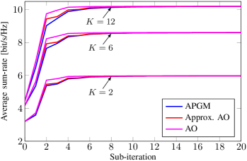
(a) Average achievable sum-rate versus the number of sub-iterations.

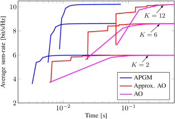
(b) Average achievable sum-rate versus the computation time.

Figure 2: Average achievable sum-rate for the proposed optimization methods with the direct and RIS-aided links.

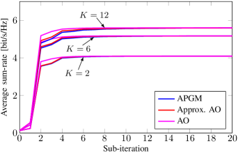
(a) Average achievable sum-rate versus the number of sub-iterations.

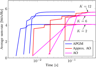
(b) Average achievable sum-rate versus the computation time.

Figure 3: Achievable sum-rate for the proposed optimization methods with the RIS-aided link only.

VI Simulation Results

In this section, we evaluate the proposed algorithms in the single-RIS and multi-RIS setups, with the aid of Monte Carlo simulations. First, in the single-RIS case, we compare the achievable sum-rates and the run times of the proposed algorithms. Furthermore, we show the variation of the achievable sum-rate with the number of transmit antennas at the BS, with the number of users, and with the number of RIS elements. We also show the change of the achievable sum-rate with the non-blockage probability of the direct links. Specifically, we consider the following three different scenarios: (i) only the direct link (i.e., the first term in (3)) is present; (ii) only the link via the RIS (i.e., the second term in (3)) is present; and (iii) both of these links are present. In the multi-RIS case, we study the change of the achievable sum-rate with the RIS positions. More specifically, this study is performed for a constant number of RIS elements per RIS and for a constant number of RIS elements in the network.

The locations of the BS, the RIS and the users are specified by a three-dimensional (3D) Cartesian coordinate system. The BS ULA is placed parallel to the y-axis and the position of its midpoint is $(0,l_{t},h_{t})$. The RIS is located in the xz-plane and the position of its midpoint is $(d_{\mathrm{ris}},0,h_{\mathrm{ris}})$. For simplicity, we assume that all of the users’ ULAs are parallel to the y-axis and the midpoint of the k-th user’s ULA is $(d_{k},l_{k},h_{k})$. For the considered system geometry, the distance between the midpoint of the BS ULA and the midpoint of the RIS is $d_{t,\mathrm{ris}}=\sqrt{d_{\mathrm{ris}}^{2}+l_{t}^{2}+(h_{t}-h_{\mathrm{ris}})^{2}}$, the distance between the midpoint of the RIS and the midpoint of the k-th user’s ULA is $d_{\mathrm{ris},k}=\sqrt{(d_{\mathrm{ris}}-d_{k})^{2}+l_{k}^{2}+(h_{\mathrm{ris}}-h_{k})^{2}}$, and the distance between the midpoint of the BS ULA and the midpoint of the k-th user’s ULA is $d_{t,k}=\sqrt{d_{k}^{2}+(l_{t}-l_{k})^{2}+(h_{t}-h_{k})^{2}}$.

In the following simulations, all the channel matrices are modeled according to the Rician fading channel model with Rician factor equal to 1, as specified in [4]. Also, we neglect the spatial correlation among the elements of matrices $\mathbf{U}$ and $\mathbf{G}_{k}$. The distance-dependent path loss for the direct link of the k-th user is $\beta_{\mathrm{DIR},k}=(4\pi/\lambda)^{2}d_{t,k}^{\alpha_{\mathrm{DIR}}}$, where $\alpha_{\mathrm{DIR}}$ denotes the path loss exponent of the direct link. The far-field free space path loss (FSPL) for the RIS-aided link of the k-th user $\beta_{\mathrm{RIS},k}$ is equal to $\beta_{\mathrm{RIS},k}^{-1}=G_{t}G_{r}\lambda^{4}\cos\gamma_{t}\cos\gamma_{r}/(256\pi^{2}d_{t,\mathrm{ris}}^{2}d_{\mathrm{ris},k}^{2})$, where $\gamma_{t}$ is the angle between the propagation direction of the incident wave and the normal to the RIS, and $\gamma_{r}$ is the angle between the normal to the RIS and the propagation direction of the reflected wave [35, Eq. (7), (9)]. Hence, we have $\cos\gamma_{t}=l_{t}/d_{t,\mathrm{ris}}$ and $\cos\gamma_{r}=l_{k}/d_{\mathrm{ris},k}$. Also, $G_{t}$ and $G_{r}$ represent the transmit and receive antenna gains respectively, which are both set to 2, since we assume that these antennas radiate/sense signals to/from the relevant half-space [35]. Finally, $\sqrt{\beta_{\mathrm{DIR},k}^{-1}/N_{0}}$ and $\sqrt{\beta_{\mathrm{RIS},k}^{-1}/N_{0}}$ are embedded as scaling factors in $\mathbf{D}_{k}$ and $\mathbf{G}_{k}$, respectively.

As for the simulation setup, the parameters are $f=2\,\mathrm{GHz}$ (i.e., $\lambda=15\,\mathrm{cm}$), $s_{t}=s_{r}=s_{\mathrm{ris}}=\lambda/2=7.5\,\mathrm{cm}$, $l_{t}=20\,\mathrm{m}$, $h_{t}=10\,\mathrm{m}$, $d_{\mathrm{ris}}=30\,\mathrm{m}$, $h_{\mathrm{ris}}=5\,\mathrm{m}$, $N_{t}=8$, $\alpha_{\mathrm{DIR}}=3$, $P=1\,\mathrm{W}$, and $N_{0}=-110\thinspace\mathrm{dB}$. The RIS consists of $N_{\mathrm{ris}}=225$ elements placed in a $15\times 15$ square formation. We assume that all users are equipped with $N_{r}=2$ antennas. The users’ coordinates are randomly selected such that $d_{k}$ is chosen from a uniform distribution between $200\,\mathrm{m}$ and $500\,\mathrm{m}$ with a resolution of $2\,\mathrm{m}$, $l_{k}$ is chosen from a uniform distribution between $1\,\mathrm{m}$ and $70\,\mathrm{m}$ with a resolution of $1\,\mathrm{m}$, and $h_{k}$ is chosen from a uniform distribution between $1.5\,\mathrm{m}$ and $2\,\mathrm{m}$ with a resolution of $1\,\mathrm{cm}$. For the dual decomposition optimization methods, we have $\mu_{\max}=KN_{t}/P$ and $\epsilon=10^{-5}$. For the gradient-based optimization methods, the initial step size value is 10000. All results are averaged over 1000 independent channel realizations.

The achievable sum-rate for the proposed methods when the channel consists of the direct and RIS-aided links, and the RIS-aided link only, are shown in Figs. 2 and 3, respectively. We assume that each iteration of Algorithms 4, 5 and 6 consists of two sub-iterations, so that in each sub-iteration we optimize all the users’ covariance matrices or all the RIS phase shifts. Hence, the achievable sum-rate in Figs. 2 and 3 is computed after every sub-iteration. For presenting the achievable sum-rate versus the rum time of the algorithms, we neglect the initial achievable sum-rate which is the same for all the algorithms and present first the achievable sum-rate obtained after the first sub-iteration. All the algorithms have the same initial values of the users’ covariance matrices and the initial values of the RIS phase shifts that are randomly generated for each channel realization. Also, all of the algorithms are executed on the same laptop computer (4 core processors with a frequency of 1.5 GHz and 16 GB RAM). From the figures, we see that the proposed optimization algorithms reach the same objective value which is a locally optimal achievable sum-rate. In addition, all the algorithms achieve the same objective value for a relatively low number of iterations. This is particularly visible for the AO algorithm. However, each iteration for the optimization of the RIS phase shifts of the AO algorithm is very time intensive because of the sequential optimization of the RIS phase shifts. In addition, the approximate AO and the APGM algorithms show approximately the same convergence behavior with respect to the number of iterations for a system with two users, while for a larger number of users the approximate AO algorithm has only a slight advantage compared to the APGM algorithm. On the other hand, the APGM algorithm requires less time to reach a locally optimal achievable rate. For a larger number of users (e.g., $K=12$) the approximate AO algorithm has almost the same convergence time as the AO algorithm. It seems that the gradient-based optimization of the users’ covariance matrices is generally more time efficient than the GBCM optimization method, especially in a system with large $K$. As expected, the achievable sum-rate in multi-user communications is higher when the direct link is present, similar to the achievable rate in point-to-point communications reported in [4]. Moreover, the achievable sum-rate increases with the number of users $K$, and the increase is more substantial when the direct link is present. It seems that the lack of capability of adjusting the amplitude of the reflection coefficients prevents the RIS from achieving a significant suppression of the multi-user interference. Therefore, higher achievable sum-rate gains can be expected when a part of a signal is transmitted via the direct link, since the BS, thanks to its amplitude adjustment capabilities, is better equipped to suppress the aforementioned interference.

In the previous setting, the APGM algorithm is shown to provide the best performance. However, as explained in Section IV-D, the convergence rate of the APGM algorithm depends on the Lipschitz constant of the gradients. Thus, the APGM algorithm is not universally the best. To illustrate this point, we consider a slightly different setting, where the number of receive antennas per user is $N_{r}=4$, the number of RIS elements is $N_{\mathrm{ris}}=100$ and $d_{k}=100\,\mathrm{m}$ for all the users. The other parameters are kept to their default values as for Fig. 3. Fig. 4 shows the achievable sum-rate of the proposed methods when only the RIS-aided link is present. Compared to Fig. 3, the number of receive antennas is larger in Fig. 4, which likely increases the Lipschitz constant of the gradients $\nabla_{\bar{\mathbf{S}}}f\bigl{(}\boldsymbol{\theta}^{(n)},\bar{\mathbf{S}}^{(n)})$ as explained analytically in Section IV-D. This in turn forces the APGM algorithm to take more iterations to converge. As can be seen in Fig. 4, the AO algorithm needs the least number of iterations and time to converge. On the other hand, the APGM algorithm requires more time and more than a magnitude of order of iterations to return a solution.

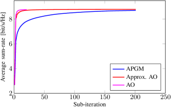
(a) Average achievable sum-rate versus the number of sub-iterations.

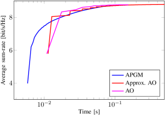
(b) Average achievable sum-rate versus the computation time.

Figure 4: Average achievable sum-rate for the proposed optimization methods with the RIS-aided link only, and slightly changed simulation parameters setup compared to Fig. 3 ($K=2$).

In the next numerical experiment, we show that the three proposed optimization algorithms can produce different sum-rate performance since the considered problem is non-convex. This justifies our motivation for proposing three algorithms for attaining the best achievable sum-rate. To this end, we consider a scenario where the are $3$ users and the number of transmit antennas is $N_{t}=4$. The users’ positions are randomly generated. The other simulation parameters are the same as those in Fig. 4. In this considered scenario, we remark that the degrees of freedom, i.e., the multiplexing gain, is very low and upper-bounded to $N_{t}=4$ . Hence, this multi-user system can transmit up to 4 independent data streams, which is equal to the maximum number of data streams for an individual user. Thus, most of the eigenvalues of $(\bar{\mathbf{S}}_{k})_{k=1}^{K}$ are 0 (i.e., the corresponding eigenchannels receive no power) to maximize the achievable sum-rate. Consequently, it becomes more challenging to find an optimal solution according to [36, Appendix A]. To illustrate this, we plot in Fig. 5 the average performance of the proposed algorithms over 100 channel realizations. For each channel realization, we also compute the best performance of the three algorithms when they are convergent, which is dubbed “Best” in Fig. 5. We notice that the algorithms achieve different sum-rates. Therefore, in systems with low degrees of freedom, all three algorithms need to be run to increase the probability that the maximum sum-rate is obtained. In general, through a large number of numerical experiments, we have observed that the APGM algorithm usually provides good trade-offs between the achievable sum-rate and complexity, and thus it is the recommended choice in most scenarios.

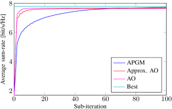
Figure 5: Average achievable sum-rate of each proposed algorithm and their best sum-rate performance.

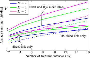
Figure 6: Achievable sum-rate versus the number of transmit antennas ($N_{t}$).

In Fig. 6, we show the achievable sum-rate for the best of the three methods versus the number of transmit antennas $N_{t}$. The achievable sum-rate has an approximately logarithmic shape. Also, it can be observed that the achievable sum-rate increases with the number of users. However, it seems that this increase gradually declines with the increase of the number of users. At the same time, the achievable sum-rate increases with the number of transmit antennas. For 6 users and 2 transmit antennas, for example, a 99 % increase in the achievable sum-rate is obtained by adding the RIS to the multi-user system.

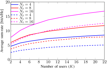
Figure 7: Average achievable sum-rate versus the number of users ($K$) in the case of direct and RIS-aided links (solid lines) and direct link only (dashed lines).

In Fig. 7, we present the achievable sum-rate for the best of the three proposed methods versus the number of users. Since we aim to investigate the increase of the achievable sum-rate due to the presence of the RIS, we show the rate in the two cases where the channel consists of the direct and RIS-aided links (solid lines), and the direct link only (dashed lines). The achievable sum-rate has an approximately logarithmic shape. In more detail, we observe that, due to the multi-user diversity gain, the achievable sum-rate is approximately proportional to $\min(N_{t},KN_{r}).$ This means that, with the increase of the number of users, the rate becomes proportional to the number of transmit antennas $N_{t}.$ Hence, the difference between the achievable sum-rates for two different values of $N_{t}$ increases with the number of users. Also, we see that the presence of the RIS increases the achievable sum-rate and influences the slope of each achievable sum-rate. Specifically, the slope of the achievable rate is slightly larger when the RIS is present, particularly for small values of $K$. As the aforementioned slope reduces with $K$, the achievable sum-rate negligibly increases for large values of $K$ when the RIS is present and the same occurs for systems without an RIS, as was already shown in [37].

In Fig. 8, we examine the benefits of DPC over linear precoding in the presence of RIS. Specifically, we plot the sum-rate versus the number of RIS elements obtained by DPC and by linear precoding. For linear precoding, we slightly modify the method introduced in [38] to find the sum-rate. Also, to understand how DPC and linear precoding perform in the case of discrete phase shifts at the RIS, we show the achievable sum-rates for DPC and linear precoding when the phase shifts are quantized with 1 or 2 bits. For these cases, the sum-rates are achieved by mapping the continuous phase shifts (when the corresponding algorithm convergences) to the closest discrete phase shift. Note that for DPC we report the best performance among the three proposed algorithms. The achievable sum-rates for DPC and linear precoding increase approximately logarithmically with the number of RIS elements. Due to the ability of DPC to presubtract the known interference, the proposed algorithms always provide a larger achievable sum-rate than the algorithm in [38]. Moreover, the performance advantage of DPC becomes more noticeable when the number of RIS elements is large. This may be attributed to the assumption that the amplitudes of the reflection coefficients of the RIS are not tunable [1]. It can also be seen that even a low resolution (i.e., 1- or 2-bit resolution) for the phase shifts of the RIS is sufficient to achieve performance comparable to the case with continuous phase shifts.

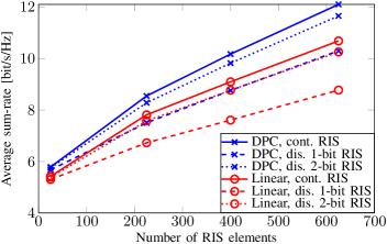
Figure 8: Average achievable sum-rates for DPC and linear precoding versus the number of quantization bits for the phase shifts of the RIS. The parameter setup is the same as for Fig. 2 and $K=6$.

Since perfect CSI is hard to obtain, particularly in RIS-aided communication systems, the achievable sum-rate subject to imperfect CSI is shown in Fig. 9. We assume that the estimated channel matrix can be represented as a sum of the true channel matrix and an estimation error matrix, which consists of i.i.d. elements that are distributed according to $\mathcal{CN}(0,\sigma^{2})$. Also, it is assumed that imperfect CSI does not influence the FSPL. We see that the achievable sum-rate exhibits a moderate decrease even for relatively large values of $\sigma^{2}$. For example, the achievable sum-rate reduces by 1.3 bit/s/Hz for $\sigma^{2}=0.9$. Hence, the proposed optimization algorithms can be efficiently used in RIS-aided communications even if the CSI knowledge is imperfect.

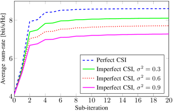
Figure 9: Achievable sum-rate assuming perfect and imperfect CSI. The parameter setup is the same as for Fig. 2 and $K=6$.

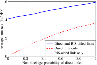
Figure 10: Average achievable sum-rate versus the non-blockage probability of the direct links ($K=2$).

In the previous simulations, we considered communication scenarios when the direct link is present or blocked. However, in most practical scenarios the direct link is blocked only for a certain fraction of time. Hence, to obtain a more comprehensive picture, Fig. 10 presents (for the case of 2 users) the achievable sum-rate versus the “non-blockage probability” of the direct links (i.e., the probability that each direct link is unblocked). Specifically, it is assumed that the non-blockage probability is the same for all users, and that the blockage of the direct link occurs independently for each user [14]. When the direct and RIS-aided links are present, the achievable sum-rate changes linearly with the non-blockage probability. When the non-blockage probability is equal to one, the achievable sum-rate boils down to the corresponding rate in Fig. 6, and when the non-blockage probability is equal zero, the achievable sum-rate is the same as when only the RIS-aided link is considered. If only the direct link is present, the achievable sum-rate has an approximately logarithmic shape and its maximum value coincides with the corresponding rate in Fig. 6.

The per-iteration computational complexities of the proposed optimization algorithms when the direct link (DL) is present or blocked are shown in Table II. The relevant numbers of iterations of the dual decomposition method $T$ and $I$, and the number of line search steps $I_{S}$ and $I_{\varTheta}$ are averaged over the first five iterations of the proposed algorithms, since all the algorithms converge within five iterations. As expected, the AO algorithm has the largest computational complexity which is mainly due to the sequential optimization of the RIS phase shifts. The approximate AO algorithm achieves a lower complexity than the AO algorithm, due to the more efficient gradient-based optimization of the RIS phase shifts. For a large number of users, the number of line search steps $I_{S}$ for the APGM algorithm is significantly lower than the total number of iterations $TI$ of Algorithm 2 for the AO and approximate AO algorithms. Therefore, the APGM algorithm is particularly suitable for application to systems with a large number of users.

DL	$K$	AO			Approximate AO				APGM
		$T$	$I$	$C_{\mathrm{AO}}$	$T$	$I$	$I_{\varTheta}$	$C_{\mathrm{A-AO}}$	$I_{S}$	$I_{\varTheta}$	$C_{\mathrm{APGM}}$
Present	2	24	3	211392	21	3	1	28368	4	1	10592
	6	26	8	540864	23	8	1	207072	4	1	28064
	12	27	14	1309248	24	14	1	720576	5	1	58240
Blocked	2	24	3	211392	21	3	1	28368	3	1	9744
	6	26	7	514656	23	7	1	183888	3	1	26448
	12	27	13	1254816	24	13	1	672192	3	2	95424

TABLE II: Comparison of the per-iteration computational complexities of the AO, approximate AO and APGM algorithms ($N_{t}=8$, $N_{r}=2$, $N_{\mathrm{ris}}=225$).

In the rest of this section, we analyze the performance of the proposed algorithms in the multi-RIS case. The simulation setup has the same parameters as in the single-RIS case except that the BS coordinate $l_{t}$ is 30 m; the $x$-coordinates $d_{k}$ are chosen from a uniform distribution between $275\,\mathrm{m}$ and $325\,\mathrm{m}$ with a resolution of $1\,\mathrm{m}$, and $l_{k}$ is chosen from a uniform distribution between $5\,\mathrm{m}$ and $55\,\mathrm{m}$ with a resolution of $1\,\mathrm{m}$ . The midpoint of the BS is aligned with the center of the user-populated area, and the distance between them is $D=300\,\mathrm{m}$. Besides the aforementioned RIS, which is denoted as RIS 1, three more RISs are added in the considered communication system. They are denoted as RIS 2, RIS 3 and RIS 4, and the positions of their midpoints are located at $(D-d_{\mathrm{ris}},0,5\thinspace\mathrm{m})$, $(d_{\mathrm{ris}},60\thinspace\mathrm{m},5\thinspace\mathrm{m})$ and $(D-d_{\mathrm{ris}},60\thinspace\mathrm{m},5\thinspace\mathrm{m})$, respectively. The achievable sum-rate for the considered system versus $d_{\mathrm{ris}}$ is presented in Fig. 11. As expected, the largest achievable rate is obtained when the RISs are located close to the BS and to the user-populated area. Interestingly, the achievable sum-rate shows only a very modest increase when RIS 1 and RIS 2 simultaneously reflect the incoming signals, as compared to the case when only one of these two surfaces performs reflection, although the number of RIS elements is doubled (i.e., it is now equal to 450). A 15 % increase in the achievable sum-rate is obtained for the RISs placed close to the center and an increase of around 35 % for the RISs placed in the vicinity of the BS and the user-populated area is obtained. This confirms the fact that the best placements for the RISs are close to the transmitter or the receiver. Similar trends can be observed when all four RISs are simultaneously reflecting the incoming signals and the total number of RIS elements is 900.

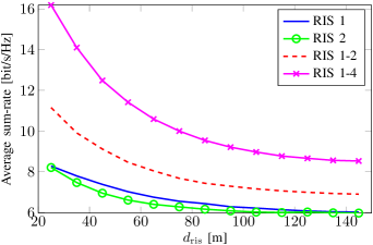
Figure 11: Average achievable sum-rates versus $d_{\mathrm{ris}}$ ($K=6$).

Lastly, we study the achievable sum-rate for the multi-RIS case where the total number of RIS elements in the system is constant. More precisely, all of the RIS elements can be located on a single RIS or equally distributed among a subset of the RISs. The achievable sum-rate when the total number of RIS elements is equal to 400 is shown in Fig. 12. Using more RISs for signal transmission is only beneficial for small values of $d_{\mathrm{ris}}$, i.e., when the RISs are in the vicinity of the BS and the user-populated area. On the other hand, the single-RIS transmission provides superior rates for larger values of $d_{\mathrm{ris}}$, i.e., when the RISs are located far from the BS and the user-populated area. It seems that placing all of the reflecting elements on a single RIS can provide a higher array gain which is essential for signal transmission via weak communication links (i.e., when the RISs are located far from the BS and the user-populated area).

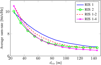
Figure 12: Average achievable sum-rates for a constant total number of RIS elements ($K=6$).

VII Conclusion

In this paper, we exploited the well-known BC-MAC duality for the achievable sum-rate optimization in a multi-user BC in the presence of one or multiple RISs. Due to the non-convexity of the considered optimization problem, we proposed three algorithms that provide the same achievable sum-rate. In the proposed algorithms, the users’ covariance matrices were optimized by a dual decomposition method with a BCM or a gradient-based method, while the optimal RIS phase shifts were sequentially computed by using a closed-form expression or in parallel by a gradient-based method. Also, we presented a computation complexity analysis for the proposed algorithms. Simulation results showed that the proposed algorithms usually achieve the same sum-rate. However, they can produce different sum-rates for some specific situations, due to the non-convexity of the considered problem. Also, the gradient-based optimization methods were generally more time efficient, particularly when the number of RIS elements is large. Furthermore, we demonstrated that the proposed algorithms are easily implementable in the multi-RIS case as well, and that can provide significant achievable sum-rate gains that depend on the placement of RIS elements in a BC.

Appendix A Computational Complexities

The complexity of the AO algorithm is determined by the computation of the covariance matrices $\{\bar{\mathbf{S}}_{k}\}_{k=1}^{K}$ and the RIS phase shifts $\{\theta_{m}\}_{m=1}^{N_{s}N_{\mathrm{ris}}}$ in Algorithm 4. At first, we need to compute all the users’ channel matrices. To compute $\mathbf{F}(\boldsymbol{\theta})\mathbf{U}$ requires $N_{\mathrm{ris}}N_{t}$ multiplications and it is common for all users. To obtain all $\mathbf{G}_{k}\mathbf{F}(\boldsymbol{\theta})\mathbf{U}$ matrices, we need $\mathcal{O}(KN_{s}N_{\mathrm{ris}}N_{t}N_{r})$ multiplications. To reduce the complexity of computing $\bar{\mathbf{H}}_{k}$, instead of implementing (16) directly, we compute and store $\mathbf{H}_{\mathrm{sum}}=\mathbf{I}+\sum_{j=1}^{K}\mathbf{H}_{j}^{{\dagger}}\bar{\mathbf{S}}_{j}\mathbf{H}_{j}$, which requires $\mathcal{O}(KN_{t}N_{r}^{2}+KN_{t}^{2}N_{r})$ multiplications. In each iteration of Algorithm 2, we first compute each gradient $\nabla_{i}\mathcal{L}\bigl{(}\mu,\bar{\mathbf{S}}^{(n)}\bigr{)}$ according to (43). The matrix inversion $\mathbf{H}_{\mathrm{sum}}^{-1}$ is executed only once per Algorithm 2 iteration, so its complexity is neglected. The product $\mathbf{H}_{k}\mathbf{H}_{\mathrm{sum}}^{-1}\mathbf{H}_{k}^{{\dagger}}$ needs $\mathcal{O}(N_{t}N_{r}^{2}+N_{t}^{2}N_{r})$ multiplications. The complexity of obtaining all $\lambda_{\max}^{2}\bigl{(}\mathbf{H}_{k}\mathbf{H}_{k}^{{\dagger}}\bigr{)}$ terms can be neglected since they can be calculated once and used in every iteration of Algorithm 2. The projection onto the semidefinite cone requires $\mathcal{O}(N_{r}^{3})$ multiplications and the complexity of line 3 of Algorithm 2 can be approximated by $\mathcal{O}(KN_{t}N_{r}^{2}+KN_{t}^{2}N_{r}+KN_{r}^{3})$. The computation of $\bar{\mathbf{H}}_{k}^{-1}=(\mathbf{H}_{\mathrm{sum}}-\mathbf{H}_{k}^{{\dagger}}\bar{\mathbf{S}}_{k}\mathbf{H}_{k})^{-1}$ has a complexity of $\mathcal{O}(N_{t}^{3})$ and the computation of $\mathbf{H}_{k}\bar{\mathbf{H}}_{k}^{-1}\mathbf{H}_{k}^{{\dagger}}$ has a complexity of $\mathcal{O}(N_{t}N_{r}^{2}+N_{t}^{2}N_{r})$. The EVD of $\mathbf{H}_{k}\bar{\mathbf{H}}_{k}^{-1}\mathbf{H}_{k}^{{\dagger}}$ requires $\mathcal{O}(N_{r}^{3})$ multiplications, while the complexity of computing $\bar{\mathbf{S}}_{k}^{(n+1)}$ is $\mathcal{O}(N_{r}^{3})$. Finally, the complexity of one iteration of Algorithm 2 is $\mathcal{O}(KN_{t}N_{r}^{2}+KN_{t}^{2}N_{r}+KN_{r}^{3})$. As a result, the computational complexity of one iteration of Algorithm 3 is $\mathcal{O}(KN_{s}N_{\mathrm{ris}}N_{t}N_{r}+TI(KN_{t}N_{r}^{2}+KN_{t}^{2}N_{r}+KN_{r}^{3}))$, where $T$ is the required number of outer iterations (i.e., lines 3 to 7) in Algorithm 3, and $I$ is the average number of iterations of Algorithm 2. In our case, $T$ is the smallest integer that satisfies the inequality $\mu_{\max}/2^{T}<\epsilon$.

The complexity of computing the optimal RIS phase shifts is primarily dependent on (22) and (23). Let us define $\mathbf{C}_{k}=\mathbf{H}_{k}-\theta_{l}\mathbf{g}_{k,l}\mathbf{u}_{l}$ to simplify the derivation. The complexity of computing the matrix $\mathbf{C}_{k}\bar{\mathbf{S}}_{k}\mathbf{C}_{k}$ is $\mathcal{O}(N_{t}N_{r}^{2}+N_{t}^{2}N_{r})$. In a similar manner, the complexity of computing $\mathbf{u}_{l}^{{\dagger}}\mathbf{g}_{k,l}^{{\dagger}}\bar{\mathbf{S}}_{k}\mathbf{g}_{k,l}\mathbf{u}_{l}$ is equal to $\mathcal{O}(N_{t}N_{r}^{2}+N_{t}^{2}N_{r})$. Hence, the complexity of computing $\mathbf{A}_{l}$ in (22) is $\mathcal{O}(KN_{t}N_{r}^{2}+KN_{t}^{2}N_{r})$. Also, we need $\mathcal{O}(KN_{t}^{2}N_{r})$ more multiplications to obtain $\mathbf{B}_{l}$ in (23). Inverting $\mathbf{A}_{l}$ requires $\mathcal{O}(N_{t}^{3})$ multiplications. The same complexity is required for computing $\mathbf{A}_{l}^{-1}\mathbf{B}_{l}$ and for obtaining the EVD of that product. The complexity of computing a single RIS phase shift is $\mathcal{O}(KN_{t}N_{r}^{2}+KN_{t}^{2}N_{r}+N_{t}^{3})$, which gives a total of $\mathcal{O}(N_{s}N_{\mathrm{ris}}(KN_{t}N_{r}^{2}+KN_{t}^{2}N_{r}+N_{t}^{3}))$ complex multiplications for the whole RIS.

In summary, the complexity of one overall iteration (i.e., lines 2 to 6 in Algorithm 4) of the AO algorithm is given by

$$C_{\mathrm{AO}}= \,\mathcal{O}(TI(KN_{t}N_{r}^{2}+KN_{t}^{2}N_{r}+KN_{r}^{3})$$

$$\;\;\;+N_{s}N_{\mathrm{ris}}(KN_{t}N_{r}^{2}+KN_{t}^{2}N_{r}+N_{t}^{3})).$$ (40)

The complexity of the approximate AO algorithm differs from the complexity of the AO algorithm in the optimization of the RIS phase shifts. To optimize the RIS phase shifts of the approximate AO algorithm, we have to calculate the gradient $\nabla_{\boldsymbol{\theta}}f\bigl{(}\boldsymbol{\theta},\bar{\mathbf{S}})$ in (28). The computation of $\mathbf{H}_{\mathrm{sum}}^{-1}\mathbf{U}^{{\dagger}}$ requires $\mathcal{O}(N_{s}N_{\mathrm{ris}}N_{t}^{2})$ complex multiplications. Since the complexity of $\mathbf{G}_{k}^{{\dagger}}\bar{\mathbf{S}}_{k}\mathbf{H}_{k}$ is $\mathcal{O}(N_{s}N_{\mathrm{ris}}N_{t}N_{r})$, the complexity of $\sum_{k=1}^{K}\mathbf{G}_{k}^{{\dagger}}\bar{\mathbf{S}}_{k}\mathbf{H}_{k}$ is $\mathcal{O}(KN_{s}N_{\mathrm{ris}}N_{t}N_{r})$. In addition, we need $\mathcal{O}(N_{s}N_{\mathrm{ris}}N_{t}^{2})$ multiplications to compute the diagonal elements of $\sum_{k=1}^{K}\mathbf{G}_{k}^{{\dagger}}\bar{\mathbf{S}}_{k}\mathbf{H}_{k}\mathbf{H}_{\mathrm{sum}}^{-1}\mathbf{U}^{{\dagger}}$. As a result, the complexity of computing the gradient $\nabla_{\boldsymbol{\theta}}f\bigl{(}\boldsymbol{\theta},\bar{\mathbf{S}})$ is $\mathcal{O}(N_{s}N_{\mathrm{ris}}N_{t}^{2}+KN_{s}N_{\mathrm{ris}}N_{t}N_{r})$. The projection $P_{\varTheta}(\cdot)$ has a negligibly small complexity. The complexity of the line search procedure assuming $I_{\varTheta}$ search steps is $\mathcal{O}(I_{\varTheta}KN_{s}N_{\mathrm{ris}}N_{t}N_{r})$. The upper-bound on $I_{\varTheta}$ corresponds to the smallest integer that satisfies the inequality $\mu_{0}/\rho^{I_{\varTheta}}<L_{\boldsymbol{\theta}}$, where $\mu_{0}$ is the initial step size and $L_{\boldsymbol{\theta}}$ is the Lipschitz constant of $\nabla_{\boldsymbol{\theta}}f(\boldsymbol{\theta},\bar{\mathbf{S}})$.

Therefore, the complexity of one overall iteration (i.e., lines 2 to 9 in Algorithm 5) of the approximate AO algorithm is given by

$$C_{\mathrm{A-AO}}= \,\mathcal{O}(TI(KN_{t}N_{r}^{2}+KN_{t}^{2}N_{r}+KN_{r}^{3})$$

$$\qquad+I_{\varTheta}KN_{s}N_{\mathrm{ris}}N_{t}N_{r}).$$ (41)

The complexity of the APGM algorithm is determined by two gradient optimization loops: one for the optimization of the covariance matrices (lines 2 to 7 in Algorithm 6) and the other for the optimization of the RIS phase shifts (lines 8 to 13 in Algorithm 6). To compute the gradient $\nabla_{\bar{\mathbf{S}}_{k}}f\bigl{(}\boldsymbol{\theta},\bar{\mathbf{S}})$ in (32), we need to calculate $\mathbf{H}_{k}\mathbf{H}_{\mathrm{sum}}^{-1}\mathbf{H}_{k}^{{\dagger}}$ which requires $\mathcal{O}(N_{t}N_{r}^{2}+N_{t}^{2}N_{r})$ multiplications. Therefore, the complexity of calculating $\nabla_{\bar{\mathbf{S}}}f\bigl{(}\boldsymbol{\theta},\bar{\mathbf{S}}\bigr{)}$ is $\mathcal{O}(KN_{t}N_{r}^{2}+KN_{t}^{2}N_{r})$. Additional $\mathcal{O}(K^{2}N_{r}^{2}+KN_{r}^{3})$ multiplications are required to calculate the projection $P_{\mathcal{S}}(\cdot)$. To compute $f(\boldsymbol{\theta}^{(n)},\bar{\mathbf{S}}^{(n+1)}),$ we need $\mathcal{O}(KN_{t}N_{r}^{2}+KN_{t}^{2}N_{r}+N_{t}^{3})$ multiplications. The additional complexity for calculating $\bar{Q}_{\bar{\mu}_{n}}(\boldsymbol{\theta}^{(n)},\bar{\mathbf{S}}^{(n+1)};\bar{\mathbf{S}}^{(n)})$ is negligible. Hence, the complexity of the line search procedure assuming $I_{S}$ search steps is $\mathcal{O}(I_{S}(KN_{t}N_{r}^{2}+KN_{t}^{2}N_{r}+N_{t}^{3}+K^{2}N_{r}^{2}))$, which is exactly the complexity of optimization loop for the covariance matrices (lines 2 to 7 in Algorithm 6). The upper-bound on $I_{S}$ corresponds to the smallest integer that satisfies the inequality $\bar{\mu}_{0}/\rho^{I_{S}}<L_{\bar{\mathbf{S}}}$, where $\bar{\mu}_{0}$ is the initial step size and $L_{\bar{\mathbf{S}}}$ is the Lipschitz constant of $\nabla_{\bar{\mathbf{S}}}f(\boldsymbol{\theta},\bar{\mathbf{S}})$. Similar to the approximate AO algorithm, the complexity of the optimization loop for the covariance matrices (lines 8 to 13 in Algorithm 6) is $\mathcal{O}(I_{\varTheta}KN_{\mathrm{ris}}N_{t}N_{r}),$ where $I_{\varTheta}$ is the number of search steps.

Therefore, the complexity of one overall iteration (lines 2 to 14 in Algorithm 6) of the APGM algorithm is equal

$$C_{\mathrm{APGM}}= \,\mathcal{O}(I_{S}(KN_{t}N_{r}^{2}+KN_{t}^{2}N_{r}+N_{t}^{3}+K^{2}N_{r}^{2})$$

$$\qquad+I_{\varTheta}KN_{s}N_{\mathrm{ris}}N_{t}N_{r}).$$ (42)

Appendix B Proof of Theorem 1

We define the partial gradient of $\mathcal{L}(\mu,\bar{\mathbf{S}})$ with respect to each component $\bar{\mathbf{S}}_{k}$ as

$$\nabla_{k}\mathcal{L}(\mu,\bar{\mathbf{S}}) =\nabla_{\bar{\mathbf{S}}_{k}}\mathcal{L}(\mu,\bar{\mathbf{S}})$$ (43a)

$$=\mathbf{H}_{k}\bigl{(}\bar{\mathbf{H}}_{k}+\mathbf{H}_{k}^{{\dagger}}\bar{\mathbf{S}}_{k}\mathbf{H}_{k}\bigr{)}^{-1}\mathbf{H}_{k}^{{\dagger}}-\mu\mathbf{I},$$ (43b)

where $\bar{\mathbf{H}}_{k}=\mathbf{I}+\sum\limits_{i=1,i\neq k}^{K}\mathbf{H}_{i}^{{\dagger}}\bar{\mathbf{S}}_{i}\mathbf{H}_{i}$. The next step is to study the Lipschitz constant of $\nabla_{k}\mathcal{L}(\mu,\bar{\mathbf{S}})$. Towards this end, let $\bar{\mathbf{S}}(\mathbf{X)}_{k}=(\bar{\mathbf{S}}_{1},\ldots\bar{\mathbf{S}}_{k-1},\mathbf{X},\bar{\mathbf{S}}_{k+1},\ldots,\bar{\mathbf{S}}_{K})$ denote the point where the $k$-th component of $\bar{\mathbf{S}}$ is replaced by $\mathbf{X}$. Then the inequalities in (46), shown at the top of the next page, hold. Thus, $\lambda_{\max}^{2}\bigl{(}\mathbf{H}_{k}\mathbf{H}_{k}^{{\dagger}}\bigr{)}$ is an upper bound for the Lipschitz constant of $\nabla_{k}\mathcal{L}(\mu,\bar{\mathbf{S}})$ and $M=\underset{1\leq k\leq K}{\max}\ \lambda_{\max}^{2}\bigl{(}\mathbf{H}_{k}\mathbf{H}_{k}^{{\dagger}}\bigr{)}$ is an upper bound for the Lipschitz constant of $\nabla\mathcal{L}(\mu,\bar{\mathbf{S}})$, which is defined as

$$\nabla\mathcal{L}(\mu,\bar{\mathbf{S}})=\bigl{(}\nabla_{1}\mathcal{L}(\mu,\bar{\mathbf{S}}),\nabla_{2}\mathcal{L}(\mu,\bar{\mathbf{S}}),\ldots,\nabla_{K}\mathcal{L}(\mu,\bar{\mathbf{S}})\bigr{)}.$$ (44)

More specifically, we have

$$\bigl{\|}\nabla\mathcal{L}(\mu,\bar{\mathbf{S}})-\nabla\mathcal{L}(\mu,\bar{\mathbf{S}}^{\prime})\bigr{\|}\triangleq\sqrt{\sum\limits\limits_{k=1}^{K}\bigl{\|}\nabla_{k}\mathcal{L}(\mu,\bar{\mathbf{S}})-\nabla_{k}\mathcal{L}(\mu,\bar{\mathbf{S}}^{\prime})\bigr{\|}^{2}}$$ (45a)

$$\leq\sqrt{\sum\limits\limits_{k=1}^{K}\lambda_{\max}^{4}\bigl{(}\mathbf{H}_{k}\mathbf{H}_{k}^{{\dagger}}\bigr{)}\bigl{\|}\bar{\mathbf{S}}_{k}-\bar{\mathbf{S}}_{k}^{\prime}\bigr{\|}^{2}}$$ (45b)

$$\leq M\sqrt{\sum\limits\limits_{k=1}^{K}\bigl{\|}\bar{\mathbf{S}}_{k}-\bar{\mathbf{S}}_{k}^{\prime}\bigr{\|}^{2}}=M\bigl{\|}\bar{\mathbf{S}}-\bar{\mathbf{S}}^{\prime}\bigr{\|}.$$ (45c)

Accordingly, Theorem 1 is a direct result of [39, Theorem 2].

$$\bigl{\|}\nabla_{k}\mathcal{L}(\mu,\bar{\mathbf{S}}(\mathbf{X)}_{k})-\nabla_{k}\mathcal{L}(\mu,\bar{\mathbf{S}}(\mathbf{Y)}_{k})\bigr{\|} =\bigl{\|}\mathbf{H}_{k}\bigl{(}\bar{\mathbf{H}}_{k}+\mathbf{H}_{k}^{{\dagger}}\mathbf{X}\mathbf{H}_{k}\bigr{)}^{-1}\mathbf{H}_{k}^{{\dagger}}-\mathbf{H}_{k}\bigl{(}\bar{\mathbf{H}}_{k}+\mathbf{H}_{k}^{{\dagger}}\mathbf{Y}\mathbf{H}_{k}\bigr{)}^{-1}\mathbf{H}_{k}^{{\dagger}}\bigr{\|}$$ (46a)

$$=\bigl{\|}\mathbf{H}_{k}\bigl{[}\bigl{(}\bar{\mathbf{H}}_{k}+\mathbf{H}_{k}^{{\dagger}}\mathbf{X}\mathbf{H}_{k}\bigr{)}^{-1}-\bigl{(}\bar{\mathbf{H}}_{k}+\mathbf{H}_{k}^{{\dagger}}\mathbf{Y}\mathbf{H}_{k}\bigr{)}^{-1}\bigr{]}\mathbf{H}_{k}^{{\dagger}}\bigr{\|}$$ (46b)

$$=\bigl{\|}\mathbf{H}_{k}\bigl{(}\bar{\mathbf{H}}_{k}+\mathbf{H}_{k}^{{\dagger}}\mathbf{X}\mathbf{H}_{k}\bigr{)}^{-1}\mathbf{H}_{k}^{{\dagger}}\bigl{(}\mathbf{X}-\mathbf{Y}\bigr{)}\mathbf{H}_{k}\bigl{(}\bar{\mathbf{H}}_{k}+\mathbf{H}_{k}^{{\dagger}}\mathbf{Y}\mathbf{H}_{k}\bigr{)}^{-1}\mathbf{H}_{k}^{{\dagger}}\bigr{\|}$$ (46c)

$$\leq\lambda_{\max}^{2}\bigl{(}\mathbf{H}_{k}\mathbf{H}_{k}^{{\dagger}}\bigr{)}\bigl{\|}\mathbf{X}-\mathbf{Y}\bigr{\|}$$ (46d)

Appendix C Proof of (26)

To simplify the notations, we write $f(\boldsymbol{\theta})$ instead of $f(\boldsymbol{\theta},\bar{\mathbf{S}})$ in this appendix. Let $\tilde{\boldsymbol{\theta}}=\begin{bmatrix}\Re(\boldsymbol{\theta})^{\mathsf{T}}&\Im(\boldsymbol{\theta})^{\mathsf{T}}\end{bmatrix}^{\mathsf{T}}$ and $\tilde{f}(\tilde{\boldsymbol{\theta}})$ be the corresponding function of real variables, i.e., $\tilde{f}(\tilde{\boldsymbol{\theta}})=f(\boldsymbol{\theta})$. From the definition of $\nabla_{\boldsymbol{\theta}}f(\boldsymbol{\theta})$, we have

$$\bigl{\|}\nabla_{\tilde{\boldsymbol{\theta}}}f(\tilde{\boldsymbol{\theta}})-\nabla_{\tilde{\boldsymbol{\theta}}}f(\tilde{\boldsymbol{\theta}}^{\prime})\bigr{\|} =2\bigl{\|}\nabla_{\boldsymbol{\theta}}f(\boldsymbol{\theta})-\nabla_{\boldsymbol{\theta}}f(\boldsymbol{\theta}^{\prime})\bigr{\|}$$

$$\leq 2L_{\boldsymbol{\theta}}(\bar{\mathbf{S}})\bigl{\|}\boldsymbol{\theta}-\boldsymbol{\theta}^{\prime}\bigr{\|}=2L_{\varTheta}\bigl{\|}\tilde{\boldsymbol{\theta}}-\tilde{\boldsymbol{\theta}}^{\prime}\bigr{\|}$$ (47)

which means that $2L_{\boldsymbol{\theta}}(\bar{\mathbf{S}})$ is the Lipschitz constant of $\nabla_{\tilde{\boldsymbol{\theta}}}f(\tilde{\boldsymbol{\theta}})$. From [32, Lemma 2.1], the following inequality holds for any $\bar{L}\geq L_{\boldsymbol{\theta}}(\bar{\mathbf{S}})$:

$$f(\boldsymbol{\theta})=\tilde{f}(\tilde{\boldsymbol{\theta}})\geq\tilde{f}(\tilde{\boldsymbol{\theta}}^{(n)})+\nabla_{\tilde{\boldsymbol{\theta}}}\tilde{f}(\tilde{\boldsymbol{\theta}}^{(n)})^{\mathsf{T}}(\tilde{\boldsymbol{\theta}}-\tilde{\boldsymbol{\theta}}^{(n)})-\frac{\bar{L}}{2}\left\|\tilde{\boldsymbol{\theta}}-\tilde{\boldsymbol{\theta}}^{(n)}\right\|^{2}$$

$$=f(\boldsymbol{\theta}^{(n)})+\nabla_{\tilde{\boldsymbol{\theta}}}\tilde{f}(\tilde{\boldsymbol{\theta}}^{(n)})^{\mathsf{T}}(\tilde{\boldsymbol{\theta}}-\tilde{\boldsymbol{\theta}}^{(n)})-\frac{\bar{L}}{2}\left\|\boldsymbol{\theta}-\boldsymbol{\theta}^{(n)}\right\|^{2}.$$ (48)

The proof is completed by letting $\mu=\frac{2}{\bar{L}}\leq\frac{1}{L_{\boldsymbol{\theta}}(\bar{\mathbf{S}})}$ and noting that $\nabla_{\tilde{\boldsymbol{\theta}}}\tilde{f}(\tilde{\boldsymbol{\theta}}^{(n)})^{\mathsf{T}}(\tilde{\boldsymbol{\theta}}-\tilde{\boldsymbol{\theta}}^{(n)})=2\Re\bigl{(}\nabla_{\boldsymbol{\theta}}f(\boldsymbol{\theta}^{(n)})^{{\dagger}}(\boldsymbol{\theta}-\boldsymbol{\theta}^{(n)})\bigr{)}=\bigl{\langle}\nabla_{\boldsymbol{\theta}}f(\boldsymbol{\theta}^{(n)}),\boldsymbol{\theta}-\boldsymbol{\theta}^{(n)}\bigr{\rangle}$.

Appendix D Convergence Analysis of the APGM Algorithm

In this appendix, we provide the convergence analysis of the proposed APGM algorithm. Our arguments follows those in [40]. Since $L_{\bar{\mathbf{S}}}(\boldsymbol{\theta}^{(n)})$ is the Lipschitz constant of $\nabla_{\bar{\mathbf{S}}}f(\bar{\mathbf{S}},\boldsymbol{\theta}^{(n)})$, it follows that

$$f(\boldsymbol{\theta}^{(n)},\bar{\mathbf{S}}^{(n+1)})\geq f(\boldsymbol{\theta}^{(n)},\bar{\mathbf{S}}^{(n)})\\ +\sum\limits_{k=1}^{K}\operatorname{Tr}\bigl{(}\bigl{(}\nabla_{\bar{\mathbf{S}}_{k}}f\bigl{(}\boldsymbol{\theta},\bar{\mathbf{S}}^{(n)})\bigr{)}\bigl{(}\bar{\mathbf{S}}_{k}^{(n+1)}-\bar{\mathbf{S}}_{k}^{(n)}\bigr{)}\bigr{)}\\ \quad-\frac{L_{\bar{\mathbf{S}}}(\boldsymbol{\theta}^{(n)})}{2}\sum_{k=1}^{K}\bigl{\|}\bar{\mathbf{S}}_{k}^{(n+1)}-\bar{\mathbf{S}}_{k}^{(n)}\bigr{\|}^{2}.$$ (49)

The projected gradient step in line 6 of Algorithm 6 implies

$$\sum\limits_{k=1}^{K}\operatorname{Tr}\bigl{(}\bigl{(}\nabla_{\bar{\mathbf{S}}_{k}}f\bigl{(}\boldsymbol{\theta},\bar{\mathbf{S}}^{(n)})\bigr{)}\bigl{(}\bar{\mathbf{S}}_{k}^{(n+1)}-\bar{\mathbf{S}}_{k}^{(n)}\bigr{)}\bigr{)}$$

$$-\frac{1}{2\mu_{n}}\sum\limits_{k=1}^{K}\bigl{\|}\bar{\mathbf{S}}_{k}^{(n+1)}-\bar{\mathbf{S}}_{k}^{(n)}\bigr{\|}^{2}\geq 0.$$ (50)

Combining (49) and (50) yields

$$f(\boldsymbol{\theta}^{(n)},\bar{\mathbf{S}}^{(n+1)})\geq f(\boldsymbol{\theta}^{(n)},\bar{\mathbf{S}}^{(n)})$$

$$+\frac{1}{2}\bigl{(}\frac{1}{\mu_{n}}-L_{\bar{\mathbf{S}}}(\boldsymbol{\theta}^{(n)})\bigr{)}\sum\limits_{k=1}^{K}\bigl{\|}\bar{\mathbf{S}}_{k}^{(n+1)}-\bar{\mathbf{S}}_{k}^{(n)}\bigr{\|}^{2}.$$ (51)

Similarly, from the $\boldsymbol{\theta}$-update we have

$$f(\boldsymbol{\theta}^{(n+1)},\bar{\mathbf{S}}^{(n+1)})\geq f(\boldsymbol{\theta}^{(n)},\bar{\mathbf{S}}^{(n+1)})\\ +\frac{1}{2}\bigl{(}\frac{1}{\bar{\mu}_{n}}-L_{\boldsymbol{\theta}}(\bar{\mathbf{S}}^{(n+1)})\bigr{)}\bigl{\|}\boldsymbol{\theta}^{(n+1)}-\boldsymbol{\theta}^{(n)}\bigr{\|}^{2}$$ (52)

and thus

$$f(\boldsymbol{\theta}^{(n+1)},\bar{\mathbf{S}}^{(n+1)})\geq f(\boldsymbol{\theta}^{(n)},\bar{\mathbf{S}}^{(n)})\\ +\frac{1}{2}\bigl{(}\frac{1}{\mu_{n}}-L_{\bar{\mathbf{S}}}(\boldsymbol{\theta}^{(n)})\bigr{)}\sum\limits_{k=1}^{K}\bigl{\|}\bar{\mathbf{S}}_{k}^{(n+1)}-\bar{\mathbf{S}}_{k}^{(n)}\bigr{\|}^{2}\\ +\frac{1}{2}\bigl{(}\frac{1}{\bar{\mu}_{n}}-L_{\boldsymbol{\theta}}(\bar{\mathbf{S}}^{(n+1)})\bigr{)}\bigl{\|}\boldsymbol{\theta}^{(n+1)}-\boldsymbol{\theta}^{(n)}\bigr{\|}^{2}.$$ (53)

The backtracking line search procedure ensures that $1/\mu_{n}\geq L_{\bar{\mathbf{S}}}(\boldsymbol{\theta}^{(n)})/\rho$ and $1/\bar{\mu}_{n}\geq L_{\boldsymbol{\theta}}(\bar{\mathbf{S}}^{(n+1)}/\rho$ which results in

$$f(\boldsymbol{\theta}^{(n+1)},\bar{\mathbf{S}}^{(n+1)})\geq f(\boldsymbol{\theta}^{(n)},\bar{\mathbf{S}}^{(n)})\\ +\frac{L_{\bar{\mathbf{S}}}(\boldsymbol{\theta}^{(n)})}{2}\bigl{(}\frac{1}{\rho}-1\bigr{)}\sum\limits_{k=1}^{K}\bigl{\|}\bar{\mathbf{S}}_{k}^{(n+1)}-\bar{\mathbf{S}}_{k}^{(n)}\bigr{\|}^{2}\\ +\frac{L_{\boldsymbol{\theta}}(\bar{\mathbf{S}}^{(n+1)})}{2}\bigl{(}\frac{1}{\rho}-1\bigr{)}\bigl{\|}\boldsymbol{\theta}^{(n+1)}-\boldsymbol{\theta}^{(n)}\bigr{\|}^{2}.$$ (54)

Since $\rho<1$, the inequality in (54) implies that the sequence $\{f(\boldsymbol{\theta}^{(n)},\bar{\mathbf{S}}^{(n)})\}$ is strictly increasing. Moreover, $f(\boldsymbol{\theta}^{(n)},\bar{\mathbf{S}}^{(n)})$ is bounded from above due to the continuity $f(\boldsymbol{\theta},\bar{\mathbf{S}})$ and the compactness of the feasible set. Hence, the objective sequence $\{f(\boldsymbol{\theta}^{(n)},\bar{\mathbf{S}}^{(n)})\}$ is convergent. Moreover, according to [40], it can be shown that the sequence $(\boldsymbol{\theta}^{(n)},\bar{\mathbf{S}}^{(n)})$ indeed converges to a stationary point of (8), but we skip the details for brevity.

References

- [1] N. S. Perović, L.-N. Tran, M. Di Renzo, and M. F. Flanagan, “On the achievable sum-rate of the RIS-aided MIMO broadcast channel,” in Proc. International Workshop on Signal Processing Advances in Wireless Communications (SPAWC). IEEE, 2021, pp. 571–575.
- [2] M. Di Renzo et al., “Smart radio environments empowered by reconfigurable AI meta-surfaces: An idea whose time has come,” EURASIP J. Wireless Commun. and Netw., vol. 2019, no. 1, pp. 1–20, 2019.
- [3] ——, “Smart radio environments empowered by reconfigurable intelligent surfaces: How it works, state of research, and road ahead,” IEEE J. Sel. Areas Commun., vol. 38, no. 11, pp. 2450–2525, Nov. 2020.
- [4] N. S. Perović et al., “Achievable rate optimization for MIMO systems with reconfigurable intelligent surfaces,” IEEE Trans. Wireless Commun., vol. 20, no. 6, pp. 3865–3882, Jun. 2021.
- [5] S. Zhang and R. Zhang, “Capacity characterization for intelligent reflecting surface aided MIMO communication,” IEEE J. Sel. Areas Commun., vol. 38, no. 8, pp. 1823–1838, Aug. 2020.
- [6] N. S. Perović et al., “Channel capacity optimization using reconfigurable intelligent surfaces in indoor mmWave environments,” in Proc. IEEE Int. Conf. on Communications (ICC), 2020, pp. 1–7.
- [7] ——, “Optimization of RIS-aided MIMO systems via the cutoff rate,” IEEE Wireless Commun. Lett., vol. 10, no. 8, pp. 1692–1696, Aug. 2021.
- [8] N. T. Nguyen et al., “Spectral efficiency optimization for hybrid relay-reflecting intelligent surface,” in Proc. IEEE Int. Conf. on Communications Workshops (ICC Workshops). IEEE, 2021, pp. 1–6.
- [9] Q. Wu and R. Zhang, “Intelligent reflecting surface enhanced wireless network via joint active and passive beamforming,” IEEE Trans. Wireless Commun., vol. 18, no. 11, pp. 5394–5409, Nov. 2019.
- [10] X. Yu et al., “Robust and secure wireless communications via intelligent reflecting surfaces,” IEEE J. Sel. Areas Commun., vol. 38, no. 11, pp. 2637–2652, Nov. 2020.
- [11] Q.-U.-A. Nadeem et al., “Asymptotic max-min SINR analysis of reconfigurable intelligent surface assisted MISO systems,” IEEE Trans. Wireless Commun., vol. 19, no. 12, pp. 7748–7764, Dec. 2020.
- [12] C. Huang et al., “Reconfigurable intelligent surface assisted multiuser MISO systems exploiting deep reinforcement learning,” IEEE J. Sel. Areas Commun., vol. 38, no. 8, pp. 1839–1850, Aug. 2020.
- [13] K. Zhi et al., “Two-timescale design for reconfigurable intelligent surface-aided massive MIMO systems with imperfect CSI,” IEEE Trans. Inf. Theory, 2022, Early access.
- [14] T. Van Chien et al., “Reconfigurable intelligent surface-assisted cell-free massive MIMO systems over spatially-correlated channels,” IEEE Trans. Wireless Commun., vol. 21, no. 7, pp. 5106–5128, Jul. 2022.
- [15] W. Ni et al., “Resource allocation for multi-cell IRS-aided NOMA networks,” IEEE Trans. Wireless Commun., vol. 20, no. 7, pp. 4253–4268, Jul. 2021.
- [16] C. Pan et al., “Multicell MIMO communications relying on intelligent reflecting surfaces,” IEEE Trans. Wireless Commun., vol. 19, no. 8, pp. 5218–5233, Aug. 2020.
- [17] Z. Zhang and L. Dai, “A joint precoding framework for wideband reconfigurable intelligent surface-aided cell-free network,” IEEE Trans. Signal Process., vol. 69, pp. 4085–4101, Jun. 2021.
- [18] C. He et al., “Multiple intelligent reflecting surfaces assisted interference coordination in multi-cell MU-MIMO communications,” arXiv preprint arXiv:2009.13899, 2020.
- [19] K. Xu et al., “On the sum-rate of RIS-assisted MIMO multiple-access channels over spatially correlated rician fading,” IEEE Trans. Commun., vol. 69, no. 12, pp. 8228–8241, Dec. 2021.
- [20] L. You et al., “Reconfigurable intelligent surfaces-assisted multiuser MIMO uplink transmission with partial CSI,” IEEE Trans. Wireless Commun., vol. 20, no. 9, pp. 5613–5627, Sep. 2021.
- [21] A. Abrardo et al., “Intelligent reflecting surfaces: Sum-rate optimization based on statistical position information,” IEEE Trans. Commun., vol. 69, no. 10, pp. 7121–7136, Oct. 2021.
- [22] B. Ning et al., “Terahertz multi-user massive MIMO with intelligent reflecting surface: Beam training and hybrid beamforming,” IEEE Trans. Veh. Technol., vol. 70, no. 2, pp. 1376–1393, Feb. 2021.
- [23] G. Caire and S. Shamai, “On the achievable throughput of a multiantenna Gaussian broadcast channel,” IEEE Trans. Inf. Theory, vol. 49, no. 7, pp. 1691–1706, Jul. 2003.
- [24] W. Yu and J. M. Cioffi, “Trellis precoding for the broadcast channel,” in Proc. GLOBECOM’01. IEEE Global Telecommunications Conference, vol. 2. IEEE, 2001, pp. 1344–1348.
- [25] S. Vishwanath et al., “Duality, achievable rates and sum-rate capacity of Gaussian MIMO broadcast channels,” IEEE Trans. Inf. Theory, vol. 49, no. 10, pp. 2658–2668, Oct. 2003.
- [26] N. Jindal et al., “Sum power iterative water-filling for multi-antenna Gaussian broadcast channels,” IEEE Trans. Inf. Theory, vol. 51, no. 4, pp. 1570–1580, Apr. 2005.
- [27] L.-N. Tran et al., “Beamformer designs for MISO broadcast channels with zero-forcing dirty paper coding,” IEEE Trans. Wireless Commun., vol. 12, no. 3, pp. 1173–1185, Mar. 2013.
- [28] S. Zhang and R. Zhang, “Intelligent reflecting surface aided multi-user communication: Capacity region and deployment strategy,” IEEE Trans. Wireless Commun., vol. 69, no. 9, pp. 5790–5806, Sep. 2021.
- [29] H. Weingarten et al., “The capacity region of the Gaussian multiple-input multiple-output broadcast channel,” IEEE Trans. Inf. Theory, vol. 52, no. 9, pp. 3936–3964, Sep. 2006.
- [30] W. Yu, “Sum-capacity computation for the Gaussian vector broadcast channel via dual decomposition,” IEEE Trans. Inf. Theory, vol. 52, no. 2, pp. 754 –759, Feb. 2006.
- [31] I. S. Dhillon et al., “Nearest neighbor based greedy coordinate descent,” in Proc. Advances in Neural Information Processing Systems 24 (NIPS 2011), 2011, pp. 1–9.
- [32] A. Beck and M. Teboulle, “A fast iterative shrinkage-thresholding algorithm for linear inverse problems,” SIAM journal on imaging sciences, vol. 2, no. 1, pp. 183–202, 2009.
- [33] X. Yu et al., “MISO wireless communication systems via intelligent reflecting surfaces,” in Proc. IEEE/CIC International Conference on Communications in China (ICCC). IEEE, 2019, pp. 735–740.
- [34] L. Condat, “Fast projection onto the simplex and the ball,” Math. Program., vol. 158, no. 1-2, pp. 575–585, Jul. 2016.
- [35] W. Tang et al., “Path loss modeling and measurements for reconfigurable intelligent surfaces in the millimeter-wave frequency band,” IEEE Trans. Commun., vol. 70, no. 9, pp. 6259–6276, Sep. 2022.
- [36] Z.-Q. Luo and S. Zhang, “Dynamic spectrum management: Complexity and duality,” IEEE J. Sel. Areas Commun., vol. 2, no. 1, pp. 57–73, Feb. 2008.
- [37] L.-N. Tran and E.-K. Hong, “Multiuser diversity for successive zero-forcing dirty paper coding: Greedy scheduling algorithms and asymptotic performance analysis,” IEEE Trans. Signal Process., vol. 58, no. 6, pp. 3411–3416, Jun. 2010.
- [38] C. Pan et al., “Intelligent reflecting surface aided MIMO broadcasting for simultaneous wireless information and power transfer,” IEEE J. Sel. Areas Commun., vol. 38, no. 8, pp. 1719–1734, Aug. 2020.
- [39] M. Hong et al., “Iteration complexity analysis of block coordinate descent methods,” Math. Program., vol. 163, no. 1, pp. 85–114, May 2017.
- [40] J. Bolte et al., “Proximal alternating linearized minimization for nonconvex and nonsmooth problems,” Math. Program., vol. 146, no. 1, pp. 459–494, 2014.