Boomerang webs up to three-loop order

Einan Gardi^a, Mark Harley, Rebecca Lodin^b, Martina Palusa^a, Jennifer M. Smillie^a, Chris D. White^c and Stephanie Yeomans

^a Higgs Centre for Theoretical Physics, School of Physics and Astronomy,
The University of Edinburgh, Edinburgh EH9 3FD, Scotland, UK

^b Department of Physics and Astronomy, Uppsala University,
Box 516, SE-75120 Uppsala, Sweden

^cCentre for Theoretical Physics, School of Physical and Chemical Sciences,
Queen Mary University of London, 327 Mile End Road, London E1 4NS, UK

Webs are sets of Feynman diagrams which manifest soft gluon exponentiation in gauge theory scattering amplitudes: individual webs contribute to the logarithm of the amplitude and their ultraviolet renormalization encodes its infrared structure. In this paper, we consider the particular class of boomerang webs, consisting of multiple gluon exchanges, but where at least one gluon has both of its endpoints on the same Wilson line. First, we use the replica trick to prove that diagrams involving self-energy insertions along the Wilson line do not contribute to the web, i.e. their exponentiated colour factor vanishes. Consequently boomerang webs effectively involve only integrals where boomerang gluons straddle one or more gluons that connect to other Wilson lines. Next we classify and calculate all boomerang webs involving semi-infinite non-lightlike Wilson lines up to three-loop order, including a detailed discussion of how to regulate and renormalize them. Furthermore, we show that they can be written using a basis of specific harmonic polylogarithms, that has been conjectured to be sufficient for expressing all multiple gluon exchange webs. However, boomerang webs differ from other gluon-exchange webs by featuring a lower and non-uniform transcendental weight. We cross-check our results by showing how certain boomerang webs can be determined by the so-called collinear reduction of previously calculated webs. Our results are a necessary ingredient of the soft anomalous dimension for non-lightlike Wilson lines at three loops.

1 Introduction

The structure of perturbative scattering amplitudes in non-Abelian gauge theories continues to be an important research area due to a wide range of phenomenological and formal applications. Of particular interest are those universal quantities in field theory that govern the all-order behaviour of amplitudes. One such quantity is the soft anomalous dimension, which controls the long-distance singularities of on-shell form factors and amplitudes. These singularities give rise to logarithms of kinematic invariants in perturbative cross-sections, which reflect incomplete cancellation between real and virtual correction, and dominate the perturbative expansion in many instances.

The soft anomalous dimension can also be determined from ultraviolet renormalization properties of correlators of Wilson-line operators [1, 2, 3, 4, 5, 6, 7]. In calculating it one must make a distinction between the colour singlet case, relevant for example for an on-shell form factor, where the singularity structure is known in full to three loops (in particular the angle-dependent cusp anomalous dimension was computed to three loops in QCD in [8, 9] and to four loops in QED in [10]), and the more complicated case of multi-leg scattering amplitudes, which is of interest here, where the soft anomalous dimension is matrix-valued in the space of possible colour flows in the underlying hard process. One must make a further distinction between lightlike Wilson lines, corresponding to the scattering of massless particles, as discussed for example in [11, 12, 13, 14, 15, 16, 17, 18, 19, 20, 21, 22, 23, 24, 25, 26, 27, 28, 29, 30, 31, 32, 33, 34, 35] and non-lightlike Wilson lines, corresponding to the scattering of heavy (coloured) particles, such as top quarks, see e.g. refs. [36, 37, 38, 39, 40, 41, 42, 43, 44, 45, 46]. In massless scattering, the soft anomalous dimension is highly constrained [22, 23, 24, 25] and it was computed in full at three-loop order [47, 48]. Furthermore, it was shown [49] that its precise form can be deduced from general considerations and special kinematic limits. These considerations do not apply directly to the massive case, and so the state-of-the-art knowledge of this quantity remains two loops [38]. While specific three-loop contributions have been directly computed in refs. [44, 45], a complete calculation is beyond the reach of present methods. In this paper, we continue the calculation of the three-loop massive soft anomalous dimension, by focusing on a particular class of contributions that have not been previously obtained.

A particularly convenient language for organising calculations involving multiple Wilson lines is that of webs, first developed in the classic work of refs. [50, 51, 52] for the two-line case. The starting point for this formalism is the fact that vacuum expectation values of Wilson lines are known to exponentiate. Crucially, the logarithm of the Wilson-line correlator can be given a Feynman diagram interpretation by itself, where the term “webs” refers to the relevant diagrams. In the two-line case in QCD, webs can be conveniently characterised by the fact that they are two-particle irreducible. Furthermore, their colour factors are modified in the logarithm of the amplitude, such that all colour factors have the property of being maximally non-Abelian, i.e. akin to the colour factors of fully connected gluon graphs. Perhaps unsurprisingly, things are more complicated in the multiparton case, and a number of formalisms have been developed [53, 54, 55, 56, 57, 58, 45, 59, 60, 61, 62, 63]. Here we will adopt the approach originated in ref. [55] (see also [64] for a review and references [65, 66] for recent progress beyond three loops), in which webs are closed sets of diagrams related by permutations of gluon attachments on the Wilson lines. Each such web is associated with a web mixing matrix describing how the colour and kinematic degrees of freedom are entangled in the logarithm of the amplitude. These matrices have a combinatorial definition that has been studied from a purely mathematical point of view [67, 68, 69], but in this paper simply provide a convenient way to organise the combination of different Feynman diagrams. The renormalization of multiparton webs has been spelled out in ref. [57], and involves combining diagrams at a given perturbative order with an intricate set of lower-order information. Furthermore, it is known that only certain combinations of diagrams survive in the logarithm of the amplitude, where each is accompanied by a fully connected colour factor [58], in direct analogy with the two-parton case.

Previously calculated three-loop webs involving massive lines include the broad class of multiple gluon exchange webs (MGEWs), defined such that the Wilson lines are connected by multiple gluon emissions, with no three- or four-gluon vertices located off the Wilson lines. Such diagrams involving four lines (the maximal number that can be connected at this order) were calculated in ref. [44]. Those involving three lines were calculated in refs. [45], where an interesting relationship with previous results was developed. Namely, it is possible to generate parts of webs connecting $n-1$ Wilson lines from those connecting $n$ lines, by taking two lines in a given $n$-line web to be collinear. The procedure can then be iterated to generate parts of webs with even fewer lines, and was dubbed collinear reduction in ref. [45]. It provides a highly nontrivial and useful consistency check of higher-loop computations, and we will encounter this idea in what follows.

References [44, 45] initiated an ongoing programme of work, to calculate all relevant diagrams for the massive three-loop soft anomalous dimension. Our aim in this study is to consider the next natural class of diagrams, namely MGEWs in which at least one gluon has both its endpoints on the same Wilson line. We shall refer to such gluons as boomerang gluons, and to the corresponding sets of diagrams containing them as boomerang webs. These were not considered in the above three-loop references, as they present additional complications related to the presence of ultraviolet divergences when the ends of a gluon meet at the same spacetime point (possibly with another gluon in between). Such complications were already present at lower orders (see e.g. [7] for a non-trivial two-loop example), but must be reconsidered here. Firstly, references [44, 45] have developed a regulator that is well-suited to isolating ultraviolet divergences in the web approach, and we will need to see how to generalise this regulator to boomerang webs. Secondly, we must account for these additional ultraviolet divergences within the general scheme developed in ref. [57] for renormalizing multiparton webs. We will deal with these issues in the following, and in turn present explicit results for all boomerang webs up to three-loop order.

Our final expressions form an important contribution to the three-loop soft anomalous dimension. In addition, we will also see a number of interesting results along the way. In particular, a large class of individual diagrams entering boomerang webs – namely those containing self-energy insertions alongside gluons which straddle multiple Wilson lines – can be proven not to appear at all, at any order in the logarithm of the Wilson-line correlator. Consequently boomerang webs spanning two or more Wilson lines effectively involve only integrals where boomerang gluons straddle one or more gluons that connect to other Wilson lines. Of course, this greatly reduces the number of integrals that need to be evaluated and simplifies the work required to assemble all contributions. Another important feature is that our final results can be written in terms of a special class of basis functions that have appeared already for MGEWs connecting four lines or fewer [44, 45], and that have been conjectured to hold for MGEWs more generally. Nevertheless, it is not a priori obvious that this class of functions would be sufficient to express boomerang webs. Indeed, while for non-boomerang MGEWs all ultraviolet divergences are associated with the renormalization of the multi-Wilson-line vertex, boomerang webs feature other divergences as well. We will see that while the former have a uniform, maximal transcendental weight of $(2n-1)$ at $n$ loops, the latter feature a lower and non-uniform weight. Despite this, we will find that the above-mentioned function basis suffices to express all boomerang webs to three loops, bolstering the expectation that it applies to this class of webs to all orders.

The structure of the paper is as follows. In section 2, we review necessary properties regarding the soft anomalous dimension and webs and their renormalization. In section 3, we consider boomerang webs at one- and two-loop order and discuss their regularisation and renormalization, preparing the grounds for the rest of the paper. In section 4 we prove the decoupling of self-energy contributions from boomerang webs to all orders in perturbation theory. In section 5, we calculate complete expressions for all three-loop boomerang webs. In section 6, we describe how collinear reduction can be used to check the consistency of parts of the results of section 5. Finally, we discuss our results and conclude in section 7. Technical details are contained in six appendices.

2 The soft anomalous dimension from webs

In this section, we review salient details regarding the web formalism that we need for the rest of the paper. We will be brief, referring the reader to refs. [55, 57, 58, 44, 45] for more details.

2.1 Wilson lines and the soft anomalous dimension

Let us first consider a Wilson-line operator associated with a semi-infinite straight-line contour:

$$\Phi_{\beta_{i}}\equiv{\cal P}\exp\left\{ig_{s}\int_{0}^{\infty}d\lambda\beta_{i}^{\mu}\,A_{\mu}(\lambda\,\beta_{i})\right\},$$ (2.1)

where $A_{\mu}$ is the gauge field, ${\cal P}$ denotes path ordering of colour generators along the Wilson-line contour, $\lambda$ is a distance parameter, and $\beta_{i}$ the 4-velocity tangent to the curve (n.b. throughout, we will be concerned with non-null Wilson lines). Our aim is to study the vacuum expectation value of a product of Wilson-line operators, and to examine its renormalization properties, for which we will use dimensional regularisation in $d=4-2\epsilon$ dimensions. However, as is well-known, Feynman diagrams involving Wilson lines vanish in dimensional regularisation, as scaleless integrals. This can be understood as an exact cancellation between ultraviolet divergences associated with the vertex (at the origin) at which the Wilson lines meet and infrared (long-distance) divergences associated with gluons emitted and absorbed at infinity. To remove the latter, we follow refs. [44, 45] in modifying each Wilson line, defining instead

$$\Phi_{\beta_{i}}^{(m)}\equiv{\cal P}\exp\left\{ig_{s}\int_{0}^{\infty}d\lambda\beta_{i}^{\mu}\,A_{\mu}(\lambda\,\beta_{i})e^{-im\lambda\sqrt{\beta_{i}^{2}-i\varepsilon}}\right\},$$ (2.2)

where $\varepsilon$ is the infinitesimal quantity appearing in the Feynman $i\varepsilon$ prescription. Here $m$ is an additional regulator that has the effect of dampening emissions with increasing distance along the Wilson line, thus smoothly removing long-distance behaviour. As has been found for previous MGEWs, and as we will see in what follows, this regulator is well-suited to the practical calculation of higher-loop webs. Armed with this regulator, we define the soft function of $L$ Wilson lines with velocities $\{\beta_{k}\}$ as

$${\cal S}\left(\gamma_{ij},\alpha_{s}(\mu^{2}),\epsilon,\frac{m}{\mu}\right)\equiv\left\langle 0\left|\Phi_{\beta_{1}}^{(m)}\otimes\Phi_{\beta_{2}}^{(m)}\otimes\ldots\otimes\Phi_{\beta_{L}}^{(m)}\right|0\right\rangle,$$ (2.3)

which depends on the $d$-dimensional coupling $\alpha_{s}(\mu^{2})$ satisfying

$$\frac{d\alpha_{s}}{d\ln\mu^{2}}=-\alpha_{s}\left[\epsilon+b_{0}\alpha_{s}+b_{1}\alpha_{s}^{2}+\ldots\right]\,,$$ (2.4)

where $\mu$ is the dimensional regularisation scale, and on the cusp angles

$$\gamma_{ij}=\frac{2\beta_{i}\cdot\beta_{j}}{\sqrt{\beta_{i}^{2}-i\varepsilon}\sqrt{\beta_{j}^{2}-i\varepsilon}}=-\left(\alpha_{ij}+\frac{1}{\alpha_{ij}}\right),$$ (2.5)

where we have defined the parameter $\alpha_{ij}$ associated with each pair of lines $i$ and $j$ for later use. We shall always pick $|\alpha_{ij}|\leq 1$. Due to the additional regulator, all singularities as $\epsilon\rightarrow 0$ are ultraviolet in origin, and the fact that multiple Wilson-line operators are multiplicatively renormalizable [3] means that we can then define the renormalized soft function

$${\cal S}_{\rm ren.}\left(\gamma_{ij},\alpha_{s}(\mu^{2}),\epsilon,\frac{m}{\mu}\right)={\cal S}\left(\gamma_{ij},\alpha_{s}(\mu^{2}),\epsilon,\frac{m}{\mu}\right)Z(\gamma_{ij},\alpha_{s}(\mu^{2}),\epsilon),$$ (2.6)

where the factor $Z$ collects all singularities associated with the renormalization of the vertex at which the Wilson lines meet. This leads to the renormalization group equation

$$\mu\frac{d}{d\mu}Z\left(\gamma_{ij},\alpha_{s}(\mu^{2}),\epsilon\right)\,=\,-\,Z\left(\gamma_{ij},\alpha_{s}(\mu^{2}),\epsilon\right)\Gamma\left(\gamma_{ij},\alpha_{s}(\mu^{2})\right)\,,$$ (2.7)

where $\Gamma$ is the soft anomalous dimension referred to above: it is a finite quantity that encapsulates the ultraviolet singularities of $Z$ and ${\cal S}$. Each of the Wilson lines $\Phi_{\beta_{k}}^{(m)}$ in eq. (2.3) carries independent colour indices in a tensor product, and thus all quantities appearing in eqs. (2.6, 2.7) must be interpreted as matrix-valued in the space of possible colour flows between the Wilson lines. As such, the order in which quantities appear on the right-hand side is important. Defining the perturbative expansion

$$\Gamma\left(\gamma_{ij},\alpha_{s}(\mu^{2})\right)=\sum_{n=1}^{\infty}\left(\alpha_{s}(\mu^{2})\right)^{n}\,\Gamma^{(n)}\left(\gamma_{ij}\right),$$ (2.8)

we may write the solution of eq. (2.7) (suppressing the dependence on the cusp angles and the scale) as

$$Z(\gamma_{ij},\alpha_{s}(\mu^{2}),\epsilon) = \exp\Bigg{\{}\alpha_{s}\,\frac{1}{2\epsilon}\,\Gamma^{(1)}+\,\alpha_{s}^{2}\left(\frac{1}{4\epsilon}\Gamma^{(2)}-\frac{b_{0}}{4\epsilon^{2}}\Gamma^{(1)}\right)$$

$$+\,\alpha_{s}^{3}\left(\frac{1}{6\epsilon}\Gamma^{(3)}+\frac{1}{48\epsilon^{2}}\left[\Gamma^{(1)},\Gamma^{(2)}\right]-\frac{1}{6\epsilon^{2}}\left(b_{0}\Gamma^{(2)}+b_{1}\Gamma^{(1)}\right)+\frac{b_{0}^{2}}{6\epsilon^{3}}\Gamma^{(1)}\right)$$

$$+\,\alpha_{s}^{4}\left(\frac{1}{8\epsilon}\Gamma^{(4)}+\frac{1}{48\epsilon^{2}}\left[\Gamma^{(1)},\Gamma^{(3)}\right]-\frac{b_{0}}{8\epsilon^{2}}\Gamma^{(3)}+\frac{1}{8\epsilon^{2}}\left(\frac{b_{0}^{2}}{\epsilon}-b_{1}\right)\Gamma^{(2)}\right.$$

$$\hskip 14.22636pt\left.-\frac{1}{8\epsilon^{2}}\left(\frac{b_{0}^{3}}{\epsilon^{2}}-\frac{2b_{0}b_{1}}{\epsilon}+b_{2}\right)\Gamma^{(1)}-\frac{b_{0}}{48\epsilon^{3}}\left[\Gamma^{(1)},\Gamma^{(2)}\right]\right)+{\cal O}\left(\alpha_{s}^{5}\right)\Bigg{\}}\,,$$

where the $\beta$-function coefficients of the $d$-dimensional coupling are defined in eq. (2.4). The unrenormalized soft function also has an exponential form, which for now we may write as

$${\cal S}\left(\alpha_{s},\epsilon\right)\,=\,\exp\Big{[}w\left(\alpha_{s},\epsilon\right)\Big{]}\,=\,\exp\left[\,\sum_{n=1}^{\infty}\,\sum_{k=-n}^{\infty}\left(\alpha_{s}(\mu^{2})\right)^{n}\,\epsilon^{k}\,w^{(n,k)}\right]\,,$$ (2.10)

i.e. $w^{(n,k)}$ collects all contributions to the logarithm of the soft function at a given order in the coupling $\alpha_{s}$, and dimensional regularisation parameter $\epsilon$. Equations (2.7) and (2.10), together with the requirement that $\Gamma^{(n)}$ be finite as $\epsilon\rightarrow 0$ imply [57]

$$\Gamma^{(1)} = -2w^{(1,-1)}\,,$$

$$\Gamma^{(2)} = -4w^{(2,-1)}-2\left[w^{(1,-1)},w^{(1,0)}\right]\,,$$

$$\Gamma^{(3)} = -6w^{(3,-1)}+\frac{3}{2}b_{0}\left[w^{(1,-1)},w^{(1,1)}\right]+3\left[w^{(1,0)},w^{(2,-1)}\right]+3\left[w^{(2,0)},w^{(1,-1)}\right]$$ (2.11)

$$+\left[w^{(1,0)},\left[w^{(1,-1)},w^{(1,0)}\right]\right]-\left[w^{(1,-1)},\left[w^{(1,-1)},w^{(1,1)}\right]\right]\,.$$

That is, the coefficients of the soft anomalous dimension are fixed from the simple pole in $\epsilon$ of the logarithm of the soft function at a given order in $\alpha_{s}=g_{s}^{2}/(4\pi)$, together with commutators (in colour space) of various coefficients at lower order. Note that the anomalous dimension coefficients must be strictly independent of the infrared cutoff scale $m$. The problem of calculating the soft anomalous dimension has now been reduced to finding the coefficients $w^{(n,k)}$ appearing in eq. (2.10). This is the subject of the following section.

2.2 Webs and their kinematic and colour factors

Equation (2.1) relates the perturbative coefficients of the soft anomalous dimension to the coefficients appearing in the logarithm of the soft function, eq. (2.10). As explained in ref. [55], we may write the total contribution $w^{(n)}$ at each loop order $n$ as a sum of webs:

$$w^{(n)}=\sum_{(n_{1},n_{2},\ldots n_{L})}w_{(n_{1},n_{2},\ldots n_{L})}^{(n)}\,,$$ (2.12)

where each web

$$W_{(n_{1},n_{2},\ldots n_{L})}\,=\,\alpha_{s}^{n}\,w_{(n_{1},n_{2},\ldots n_{L})}^{(n)}=\alpha_{s}^{n}\sum_{k=-n}^{\infty}\epsilon^{k}w_{(n_{1},n_{2},\ldots n_{L})}^{(n,k)}\,,$$ (2.13)

consists of a closed set of diagrams connecting $L$ Wilson lines, with a fixed number of gluon attachments $(n_{1},n_{2},\ldots,n_{L})$ on each line, where $n_{i}\geq 0$. The diagrams in a single web are interrelated by all possible permutations of the gluon attachments along each Wilson line. Each diagram $D\in W_{(n_{1},\ldots,n_{L})}$ has a colour factor $C(D)$ and kinematic part ${\cal F}(D)$, such that the contribution of the web to $w^{(n)}$ may be written in the form

$$W=\sum_{D,D^{\prime}\in W}{\cal F}(D)R_{DD^{\prime}}{\cal C}(D^{\prime}).$$ (2.14)

The quantity $R_{DD^{\prime}}$ (a matrix in the space of diagrams) is called a web mixing matrix, and has a purely combinatorial definition. An algorithm to calculate the mixing matrix for a given web was given in ref. [55], further combinatorial aspects have been explored in refs. [67, 68, 69], and recent progress beyond three loops was reported in refs. [65, 66]. Physically, the web mixing matrix describes how colour and kinematic factors are entangled in the logarithm of the soft function.

Although a full understanding of web mixing matrices remains elusive, some general properties have been well-established. Chief among these is the fact that web mixing matrices are idempotent, and thus act as projection operators, with eigenvalues $\lambda_{i}\in\{0,1\}$. The rank $r$ of a $p$-dimensional web mixing matrix is the number of unit eigenvalues. Let $Y$ be the matrix that diagonalises the web mixing matrix:

$$YRY^{-1}={\rm diag}(\lambda_{1},\lambda_{2},\ldots\lambda_{p}),\qquad\lambda_{i}=\begin{cases}1,\quad i\leq r;\\ 0,\quad r+1\leq i\leq p.\end{cases}$$ (2.15)

Then we can write the contribution of a single web as

$$W=\sum_{j=1}^{r}\left(\sum_{D}{\cal F}(D)Y^{-1}_{D,j}\right)\left(\sum_{D^{\prime}}Y_{j,D^{\prime}}C(D^{\prime})\right)\equiv\sum_{j=1}^{r}{\cal F}_{W;j}^{(n)}c_{j}^{[n,L]}\,.$$ (2.16)

As expressed by the second equality, this has the form of a sum over combinations of kinematic factors ${\cal F}_{W;\,j}^{(n)}$ (one for each unit eigenvalue), each accompanied by a corresponding colour factor $c_{j}^{[n,L]}$, where $n$ indicates the loop order and $L$ denotes the number of Wilson lines. It has now been proven [58] that each such colour factor is equivalent to the colour factor of a fully connected soft gluon graph. As mentioned above, this is the appropriate generalisation of the maximally non-Abelian property of two-line webs [50, 51, 52] to the multiparton case. We will briefly discuss our basis of these connected colour factors in section 2.3 below.

Having introduced the colour decomposition of each web in eq. (2.16), we may write the corresponding Laurent expansion in $\epsilon$, eq. (2.13), more explicitly as

$$W_{(n_{1},n_{2},\ldots n_{L})}=\alpha_{s}^{n}w_{(n_{1},n_{2},\ldots n_{L})}^{(n)}=\alpha_{s}^{n}\sum_{k=-n}^{\infty}\epsilon^{k}w_{(n_{1},n_{2},\ldots n_{L})}^{(n,k)}=\sum_{j=1}^{r}{\cal F}^{(n)}_{(n_{1},n_{2},\ldots n_{L});j}c_{j}^{[n,L]}\,.$$ (2.17)

To obtain the contributions of a given $n$-loop web to $w^{(n,k)}$ of eq. (2.12) we must therefore expand its kinematic function ${\cal F}^{(n)}_{(n_{1},n_{2},\ldots n_{L});j}$ in $\epsilon$:

$${\cal F}^{(n)}_{(n_{1},n_{2},\ldots n_{L});j}=\sum_{k=-n}^{\infty}\epsilon^{k}{\cal F}^{(n,k)}_{(n_{1},n_{2},\ldots n_{L});j}\,,$$ (2.18)

and then recast the result as

$$w_{(n_{1},n_{2},\ldots n_{L})}^{(n,k)}=\sum_{j=1}^{r}{\cal F}^{(n,k)}_{(n_{1},n_{2},\ldots n_{L});j}c_{j}^{[n,L]}\,.$$ (2.19)

In order to express the anomalous dimension in eq. (2.1) at order $n$ in the loop expansion we need, specifically, the single pole terms ($k=-1$) of each web. It is convenient to write

$$\Gamma^{(n)}=-2n\,\overline{w}^{(n,-1)},\qquad\quad\overline{w}^{(n,-1)}=\!\!\sum_{(n_{1},n_{2},\ldots n_{L})}\!\!\overline{w}_{(n_{1},n_{2},\ldots n_{L})}^{(n,-1)}$$ (2.20)

where we followed refs. [44, 45] in defining subtracted webs $\overline{w}$ which include, for each web, the commutators of the relevant web-subdiagrams taken at ${\cal O}(\epsilon^{-1})$, according to eq. (2.1). For example, for three-line webs at two loops, according to the second relation in eq. (2.1) the subtracted $(1,1,2)$ web is defined as

$$\overline{w}_{(1,1,2)}^{(2,-1)}=w_{(1,1,2)}^{(2,-1)}+\frac{1}{2}\left[w_{(1,0,1)}^{(1,-1)},\,w_{(0,1,1)}^{(1,0)}\right]+\frac{1}{2}\left[w_{(1,1,0)}^{(1,-1)},\,w_{(1,0,1)}^{(1,0)}\right]\,.$$ (2.21)

The colour decomposition of each subtracted web in eq. (2.20) readily follows from eq. (2.19):

$$\overline{w}_{(n_{1},n_{2},\ldots n_{L})}^{(n,-1)}\,=\,\sum_{j=1}^{r}\overline{w}_{(n_{1},n_{2},\ldots n_{L});j}^{(n,-1)}\,=\,\left(\frac{1}{4\pi}\right)^{n}\,\sum_{j=1}^{r}F^{(n)}_{(n_{1},n_{2},\ldots n_{L});j}c_{j}^{[n,L]}\,,$$ (2.22)

where the $\{F^{(n)}_{(n_{1},n_{2},\ldots n_{L});j}\}$ carry the kinematic dependence on the Wilson-line velocities associated with the colour structure $j$. These kinematic functions are independent of both the infrared cutoff scale $m$ and the dimensional regulator and they directly contribute to the anomalous dimension, eq. (2.20). Their calculation – for the case of boomerang webs – will be a central goal of the present paper.

2.3 Web colour bases

Given that any superposition of degenerate eigenvectors of the web mixing matrix is also an eigenvector, the matrix $Y$ in eq. (2.16) is not unique. Put another way, the basis of colour factors $c_{j}^{[n,L]}$ is also not unique, and one must choose a suitable basis before calculating all webs at a given order. One such basis was presented in ref. [58], which developed an alternative language for the logarithm of the soft function. That is, one may think of the latter as consisting of diagrams composed of effective vertices $\{V_{K}^{(l)}\}$, describing the emission of $K$ gluons from the specific Wilson line $l$. In general there can be several such vertices on a given line, but such that their respective position along the line is fully symmetrised. The colour factor associated with each such vertex is that of a fully connected gluon configuration. For example, the case of two gluons has only the single possibility

$$C_{2,1}^{ab}=\left[T^{a},T^{b}\right]=if^{abc}T^{c},$$ (2.23)

which is the same as the colour factor associated with a gluon emitted from the Wilson line, that then splits into two via a three-gluon vertex. For three gluons, there are two independent connected colour factors, namely

$$C_{3,1}^{ab,c}=\left[\left[T^{a},T^{b}\right],T^{c}\right]=f^{abd}f^{ecd}T^{e};$$

$$C_{3,2}^{ac,b}=\left[\left[T^{a},T^{c}\right],T^{b}\right]=f^{acd}f^{ebd}T^{e}.$$ (2.24)

Ref. [58] showed that any connected diagram – i.e. one that remains connected when the Wilson lines themselves are removed – composed of such vertices on the Wilson lines, and ordinary QCD vertices off the Wilson lines, has a connected (“maximally non-Abelian”) colour factor. In this way the effective-vertex formalism was used in establishing the non-Abelian exponentiation theorem for multiple Wilson lines. Furthermore, this formalism provides a neat way to fix a suitable colour basis for webs. For a given web $W_{(n_{1},n_{2},\ldots,n_{L})}$, the possible connected colour factors are generated by the possible assignments of effective vertices on each Wilson line, commensurate with the gluon attachment numbers $\{n_{i}\}$. As explained in ref. [58], if more than one effective vertex is present on a given line, one determines the contribution of this line to the overall colour factor by fully symmetrising over the individual vertex colour factors $\{C_{i}\}$:

$$\left\{C_{1}\,C_{2}\ldots C_{n}\right\}_{+}\equiv\frac{1}{n!}\sum_{\pi\in S_{n}}C_{\pi_{1}}\,C_{\pi_{2}}\ldots C_{\pi_{n}}.$$ (2.25)

We can use this to formulate a basis for the overall connected colour factors of webs connecting $L$ lines as follows. Firstly, let us denote by $\{C_{K,j}(l)\}$ the set of $(K-1)!$ independent colour factors associated with a given effective vertex $V_{K}^{(l)}$ on Wilson line $l$ (examples are given in eqs. (2.23, 2.24)). Then a fully general web colour basis is provided by the colour factors

$$c_{j}^{[n,L]}=\prod_{l=1}^{L}\left\{C_{K_{1},j_{1}}{(l)}\,C_{K_{2},j_{2}}{(l)}\ldots C_{K_{n_{l}},j_{n_{l}}}{(l)}\right\}_{+},$$ (2.26)

consisting of the different choices of effective vertex factors multiplied together on each line, and symmetrised according to eq. (2.25). The effective vertex colour matrix $C_{K,j}{(l)}$ carries $K$ adjoint indices, which may be contracted in (2.26) with those of other colour matrices on any of the Wilson lines. In particular, we will be interested in this paper in boomerang webs where there are contractions between the adjoint indices of pairs of effective vertex colour matrices on the same line. As noted already in ref. [58], in this case the basis defined by eq. (2.26) is expected to be over-complete: there may be linear relations between $c_{j}^{[n,L]}$ consisting of different sets of vertices $C_{K,j}{(l)}$, all having the same total number of gluons emitted from line $l$ (out of which some pairs are contracted to form boomerang gluons). This will become important in section 6.2 (see eqs. (6.10) and (6.25) there) where we will study a related, highly non-trivial relation between webs spanning a different number of Wilson lines upon taking collinear limits.

2.4 Kinematic factors of MGEWs

Having addressed the colour structure of webs in the previous sections, we must also describe how to calculate the kinematic part ${\cal F}(D)$ of a web diagram $D$. References [44, 45] developed a systematic procedure for calculating the kinematic parts of multiple gluon exchange webs, that will provide a highly useful starting point for what follows. First, we will use the Feynman gauge gluon propagator in configuration space, which in $d=4-2\epsilon$ dimensions is

$${\cal D}_{\mu\nu}(x)=-{\cal N}\eta_{\mu\nu}(-x^{2}+i\varepsilon)^{\epsilon-1},$$ (2.27)

where

$${\cal N}=\frac{\Gamma(1-\epsilon)}{4\pi^{2-\epsilon}}.$$ (2.28)

Furthermore, eq. (2.2) implies that the Feynman rule for emission of a gluon from a Wilson line is

$$ig_{s}\bar{\mu}^{\epsilon}\,\int_{0}^{\infty}d\lambda\beta_{i}^{\mu}e^{-im\lambda\sqrt{\beta_{i}^{2}-i\varepsilon}}.$$ (2.29)

These results are sufficient to calculate any MGEW, given (by definition) the absence of three- or four-gluon vertices located off the Wilson lines. Let us now consider such a web, consisting of $n$ individual gluon exchanges, where the $k^{\rm th}$ such gluon straddles the Wilson lines $i(k)$ and $j(k)\neq i(k)$ (i.e. we do not yet allow for the possibility of boomerang gluons). Letting $s_{k}$ and $t_{k}$ denote the distance parameters of the gluon along these two Wilson lines, the expression for a given web diagram $D$ is given by

$${\cal F}^{(n)}(D) =(g_{s}^{2}\,\bar{\mu}^{2\epsilon}\,{\cal N})^{n}\prod_{k=1}^{n}\left(\beta_{i(k)}\cdot\beta_{j(k)}\int_{0}^{\infty}ds_{k}dt_{k}\right)\,\prod_{k=1}^{n}\left[-(\beta_{i(k)}s_{k}-\beta_{j(k)}t_{k})^{2}+i\varepsilon\right]^{-1+\epsilon}$$

$$\quad\times\,\Theta_{D}[\{s_{k},t_{k}\}]\,\exp\left[-im\sum_{k=1}^{n}\left(s_{k}\sqrt{\beta_{i(k)}^{2}-i\varepsilon}+t_{k}\sqrt{\beta_{j(k)}^{2}-i\varepsilon}\right)\right].$$ (2.30)

Here $\Theta_{D}[\{s_{k},t_{k}\}]$ consists of a product of Heaviside functions involving the distance parameters, that implements the ordering of the gluons on each Wilson line. To carry out the integrals in eq. (2.30), one may first rescale to

$$\sigma_{k}=s_{k}\sqrt{\beta_{i(k)}^{2}},\quad\tau_{k}=t_{k}\sqrt{\beta_{j(k)}^{2}},$$ (2.31)

before changing variables according to

$$\sigma_{k}=x_{k}\lambda_{k},\quad\tau_{k}=(1-x_{k})\lambda_{k};\qquad 0\leq\lambda_{k}\leq\infty,\quad 0\leq x_{k}\leq 1,$$ (2.32)

where $\lambda_{k}$ measures how far a given gluon is from the origin (the hard interaction vertex, where the Wilson lines meet), and $x_{k}$ is an “angular” variable, which tends to 0 or 1 in the limits where the gluon is collinear with line $i(k)$ or $j(k)$ respectively. Equation (2.30) then becomes

$${\cal F}^{(n)}\left(D\right) = \,\left(\frac{1}{2}\,g_{s}^{2}\bar{\mu}^{2\epsilon}\,\frac{\Gamma(1-\epsilon)}{4\pi^{2-\epsilon}}\right)^{n}\,\prod_{k=1}^{n}\Bigg{[}\int_{0}^{\infty}d\lambda_{k}\,\lambda_{k}^{-1+2\epsilon}\,{\rm e}^{-i(m-i\varepsilon)\lambda_{k}}$$

$$\times\,\,\int_{0}^{1}dx_{k}\,\gamma_{k}\,\Big{[}-x_{k}^{2}-(1-x_{k})^{2}+\gamma_{k}\,x_{k}(1-x_{k})+i\varepsilon\Big{]}^{-1+\epsilon}\Bigg{]}\,\Theta_{D}\big{[}\left\{x_{k},\lambda_{k}\right\}\big{]}\,,$$

where $\gamma_{k}\equiv\gamma_{i(k)j(k)}$ is the cusp angle between lines $i(k)$ and $j(k)$, as defined in eq. (2.5). To proceed, one may define

$$\lambda_{k}\,=\,\left(1-y_{k-1}\right)\,\prod_{p=k}^{n}y_{p}\,,\quad k=1,\ldots,n,\quad y_{0}=0,$$ (2.34)

so that the exponential-regulator factor simplified to ${\rm e}^{-i(m-i\varepsilon)y_{n}}$, and after integrating over $y_{n}$, eq. (2.4) becomes (see ref. [45] for more details):

$${\cal F}^{(n)}\left(D\right) = \kappa^{n}\,\Gamma(2n\epsilon)\,\,\prod_{k=1}^{n}\Bigg{[}\int_{0}^{1}dx_{k}\,\gamma_{k}\,\Big{[}x_{k}^{2}+(1-x_{k})^{2}-\gamma_{k}\,x_{k}(1-x_{k})\Big{]}^{-1+\epsilon}\Bigg{]}$$ (2.35)

$$\hskip 42.67912pt\times\,\,\prod_{k^{\prime}=1}^{n-1}\Bigg{[}\int_{0}^{1}dy_{k^{\prime}}\left(1-y_{k^{\prime}}\right)^{-1+2\epsilon}\,y_{k^{\prime}}^{-1+2k^{\prime}\epsilon}\Bigg{]}\,\,\,\Theta_{D}\big{[}\left\{x_{k},y_{k^{\prime}}\right\}\big{]}$$

$$= \kappa^{n}\,\,\Gamma(2n\epsilon)\,\prod_{k=1}^{n}\bigg{[}\int_{0}^{1}dx_{k}\,\gamma_{k}\,P_{\epsilon}\left(x_{k},\gamma_{k}\right)\bigg{]}\,\phi_{D}^{(n)}\left(x_{i};\epsilon\right)\,,$$

where we have defined the expansion parameter

$$\kappa\,\equiv-\frac{1}{2}\,g_{s}^{2}\left(\frac{\bar{\mu}^{2}}{m^{2}}\right)^{\epsilon}\,\frac{\Gamma(1-\epsilon)}{4\pi^{2-\epsilon}}\,,$$ (2.36)

which is convenient at intermediate stages of the calculation. In the second line in eq. (2.35) we also defined the propagator-related function

$$P_{\epsilon}\left(x,\gamma\right)\,\equiv\,\left[x^{2}+(1-x)^{2}-x(1-x)\gamma)\right]^{-1+\epsilon}\,$$ (2.37)

and the kernel of diagram $D$

$$\phi_{D}^{(n)}\left(x_{i};\epsilon\right)\,=\,\prod_{k=1}^{n-1}\Bigg{[}\int_{0}^{1}dy_{k}\left(1-y_{k}\right)^{-1+2\epsilon}\,y_{k}^{-1+2k\epsilon}\Bigg{]}\,\,\Theta_{D}\big{[}\left\{x_{i},y_{i}\right\}\big{]}\,,$$ (2.38)

consisting of integrals over Heaviside functions originating from the ordering of gluon attachments. At this point it is natural to perform the integrals defining the kernel for each diagram, expanded as a Laurent series in $\epsilon$, obtaining $\phi_{D}^{(n)}$ in terms of logarithms and polylogarithms of the variables $\{x_{i}\}$. In eq. (2.35), the kernel will eventually be integrated over the variables $\{x_{i}\}$ after multiplying it with the functions $P_{\epsilon}(x_{i},\gamma_{i})$ related to the gluon propagators. The overall divergence in the factor $\Gamma(2n\epsilon)$ in eq. (2.35) is associated with the ultraviolet divergence one obtains upon shrinking the entire soft gluon diagram $D$ to the origin [44, 45].

All diagrams within a given web (i.e. with the same numbers of gluon attachments at a given perturbative order) will have an integral expression of the form of eq. (2.35). The only difference between such diagrams will be the kernel of eq. (2.38), which is the only part sensitive to the ordering of gluons on the Wilson lines. It then follows from section 2.2 that the contribution of a web $W$ to the colour structure $c_{j}^{[n,L]}$ in our chosen basis is given by

$${\cal F}_{W;\,j}^{(n)}\left(\gamma_{ij},\epsilon\right)\,=\,\kappa^{n}\,\Gamma(2n\epsilon)\,\prod_{k=1}^{n}\bigg{[}\int_{0}^{1}dx_{k}\,\gamma_{k}\,P_{\epsilon}\left(x_{k},\gamma_{k}\right)\bigg{]}\,\phi_{W,\,j}^{(n)}\left(x_{i};\epsilon\right)\,,$$ (2.39)

where, following eq. (2.16), the web kernel is defined by

$$\phi^{(n)}_{W,\,j}\left(x_{i};\epsilon\right)\,=\,\sum_{D\in W}Y_{D,j}^{-1}\,\phi^{(n)}_{D}\left(x_{i};\epsilon\right)\,.$$ (2.40)

As an example, we collect in appendix A the final results for the kinematic factors $\{{\cal F}^{(n)}_{W}\}$ of one- and two-loop MGEWs, after integration over the $\{y_{k}\}$ variables of eq. (2.38). Similar three-loop results can be found in refs. [44, 45]. The integrals over the variables $\{x_{k}\}$ in (2.40) could in principle also be carried out at this stage. However, in forming the soft anomalous dimension, one must combine the result for each web with commutators of its web-subdiagrams, as prescribed by eq. (2.1), leading to the definition of subtracted webs in eq. (2.20). It turns out that performing the integrals over the $\{x_{k}\}$ variables at the level of the subtracted webs is also much easier to carry out than for the web itself. This was explained in refs. [44, 45], showing that for subtracted webs this integration yields a highly restricted class of functions, which we briefly recall below.

Following refs. [44, 45], we write each ${\cal O}(\alpha_{s}^{n})$ subtracted web as in eq. (2.22), namely

$$\overline{w}^{(n,-1)}\left(\alpha_{k}\right)\,=\,\left(\frac{1}{4\pi}\right)^{n}\,\sum_{j=1}^{r}\,c_{j}^{[n,L]}\,F^{(n)}_{W;\,j}\big{(}\alpha_{k}\big{)}\,,$$ (2.41)

where from eqs. (2.5) we define $\gamma_{k}=-\alpha_{k}-1/\alpha_{k}$. Essential to deriving the subtracted web of eq. (2.41) is the fact that the commutators in eq. (2.1) build up the same fully connected colour factors as in the chosen basis of section 2.3. The kinematic function multiplying each colour structure, $F^{(n)}_{W;\,j}$, contains integrals over the variables $\{x_{k}\}$, as well as the propagator functions of eq. (2.37), rewritten in terms of $\alpha$:

$$\begin{split}&p_{\epsilon}\left(x,\alpha\right)\,\equiv\gamma\,P_{\epsilon}\left(x,\gamma\right)=\,-\,\left(\alpha+\frac{1}{\alpha}\right)\,\Big{[}q(x,\alpha)\Big{]}^{-1+\epsilon}\,\\ &q\left(x,\alpha\right)\,\equiv\,x^{2}+(1-x)^{2}+\left(\alpha+\frac{1}{\alpha}\right)\,x(1-x)\,=-\frac{(1-\alpha)^{2}}{\alpha}\left(x-\frac{1}{1-\alpha}\right)\left(x+\frac{\alpha}{1-\alpha}\right)\,.\end{split}$$ (2.42)

The factorization property of $q\left(x,\alpha\right)$ clarifies the advantage of using the variable $\alpha$ over using $\gamma$ (see also ref. [70]). This ultimately amounts to rationalising the symbol alphabet. The integrals may be carried out after expansion in the dimensional regularisation parameter $\epsilon$, for which eq. (2.42) becomes

$$p_{\epsilon}\left(x,\alpha\right)\,=\,p_{0}\left(x,\alpha\right)\,\sum_{n=0}^{\infty}\frac{\epsilon^{n}}{n!}\Big{[}\log q\left(x,\alpha\right)\Big{]}^{n}\,,$$ (2.43)

where

$$p_{0}\left(x,\alpha\right)\,=\,-\,\left(\alpha+\frac{1}{\alpha}\right)\,\frac{1}{q(x,\alpha)}\,=\,r(\alpha)\left[\frac{1}{x-\frac{1}{1-\alpha}}-\frac{1}{x+\frac{\alpha}{1-\alpha}}\right]\,,$$ (2.44)

is the leading part of the propagator function as $\epsilon\rightarrow 0$, and we have defined the rational prefactor

$$r(\alpha)\,=\,\frac{1+\alpha^{2}}{1-\alpha^{2}}\,.$$ (2.45)

Finally, the subtracted web kinematic factor can be written as

$$F^{(n)}_{W;\,j}\big{(}\alpha_{i}\big{)} = \prod_{k=1}^{n}\left[\int_{0}^{1}\,dx_{k}\,p_{0}(x_{k},\alpha_{k})\right]\,{\cal G}^{(n)}_{W;\,j}\Big{(}x_{i},q(x_{i},\alpha_{i})\Big{)}\,$$ (2.46)

$$= \,\left(\prod_{k=1}^{n}r(\alpha_{k})\right)\prod_{k=1}^{n}\left[\int_{0}^{1}dx_{k}\left(\frac{1}{x_{k}-\frac{1}{1-\alpha_{k}}}-\frac{1}{x_{k}+\frac{\alpha_{k}}{1-\alpha_{k}}}\right)\right]\,{\cal G}^{(n)}_{W;\,j}\Big{(}x_{i},q(x_{i},\alpha_{i})\Big{)}\,$$

$$\equiv \,\left(\prod_{k=1}^{n}r(\alpha_{k})\right)G^{(n)}_{W;\,j}\big{(}\alpha_{i}\big{)}\,,$$

which defines the subtracted web kernel ${\cal G}_{W;j}^{(n)}$, and its fully integrated counterpart $G_{W;j}^{(n)}$. In all previously studied MGEWs [44, 45], the subtracted web kernel consists exclusively of powers of logarithms of certain rational functions of $x_{k}$ and $\alpha_{k}$ (details will follow). The integrals in the middle line of eq. (2.46) are then in so-called $d\log$ form, and can be carried out explicitly to give $G^{(n)}_{W;\,j}\big{(}\alpha_{i}\big{)}$ as a pure transcendental function of weight $(2n-1)$, consisting of a sum of products of harmonic polylogarithms, where a given polylogarithm depends on a single angle $\alpha_{ij}$. More than this, the functions appearing in the final answer are of a special type, as we review in the following section. As stated above, we have considered here only webs that do not contain boomerang gluons i.e. all gluon exchanges begin and end on different Wilson lines. We will need to generalise the above results to cope with the case when boomerang gluons are indeed present.

2.5 A basis of functions for MGEWs

Upon integrating the subtracted web kernel for a given MGEW, one obtains a pure transcendental function $G^{(n)}_{W;\,j}$ taking the form of a sum of products of harmonic polylogarithms of $\alpha_{ij}$, where each polylogarithm depends on a single $\alpha_{ij}$. The analytic properties of such functions can be efficiently encoded by means of the symbol map [71, 72, 73, 74]. It was argued already in ref. [44] that the symbol of (integrated) subtracted MGEWs has the highly restricted alphabet

$$\left\{\alpha_{ij},\quad\eta_{ij}\equiv\frac{\alpha_{ij}}{1-\alpha_{ij}^{2}}\right\}\,.$$ (2.47)

This structure realises the two symmetries

$$\alpha\to-\alpha\qquad{\rm and}\qquad\alpha\to\frac{1}{\alpha}$$ (2.48)

at symbol-level. Reference [45] then proposed a set of basis functions consistent with this symbol alphabet, and in terms of which all currently calculated MGEWs can be expressed. To quote the basis, we may use the functions defined in the previous section, as well as the additional function $\tilde{q}(x,\alpha)$ given by

$$\ln\tilde{q}(x,\alpha)\,\equiv\,\frac{1}{r(\alpha)}\int_{0}^{1}dy\,p_{0}(y,\alpha)\theta(x>y)\,=\ln\left(\frac{1}{x}+\alpha-1\right)-\ln\left(\frac{1}{x}+\frac{1}{\alpha}-1\right)\,.$$ (2.49)

The proposed basis for $G^{(n)}_{W;\,j}$ in eq. (2.46) can then be written as

$$M_{k,l,n}(\alpha)\,=\,\frac{1}{r(\alpha)}\int_{0}^{1}dx\,p_{0}(x,\alpha)\ln^{k}\bigg{(}\frac{q(x,\alpha)}{x^{2}}\bigg{)}\ln^{l}\bigg{(}\frac{x}{1-x}\bigg{)}\ln^{n}\tilde{q}(x,\alpha)\,,$$ (2.50)

where each function in the set has uniform weight ${\rm w}=k+l+n+1$. Defined in this manner, the basis is actually overcomplete, as the functions satisfy the relations

$$M_{k,l,n}(\alpha)\,=\,(-1)^{l+n}\sum_{r=0}^{k}\sum_{s=0}^{n}\left(\begin{array}[]{c}k\\ r\end{array}\right)\left(\begin{array}[]{c}n\\ s\end{array}\right)2^{s+r}(-1)^{s}\log^{s}(\alpha)\,M_{k-r,l+r,n-s}(\alpha)\,.$$ (2.51)

For completeness, we quote the symbols of basis functions which occur up to three-loop order – as well as explicit forms for the functions themselves – in appendix B. There is currently much evidence that this basis is sufficient for describing MGEWs to all orders in perturbation theory. Up to three-loop order, it covers all such webs that do not involve boomerang gluons [44, 45], including those two-line webs that involve intricate patterns of crossed gluon exchanges. Furthermore, a certain special diagram type, called the Escher staircase in ref. [45], can be calculated for arbitrary numbers of gluon exchanges, and is fully expressible in terms of the basis of eq. (2.50). It remains to be seen whether or not the basis will cope if boomerang gluons are indeed present, and it is one of the aims of the present paper to explore this.

Note that one of the simplifying features of subtracted web kernels, discussed in detail in refs. [44, 45], is that higher weight polylogarithm functions (such as dilogs) are absent, whereas they are present in the web kernel itself. This made it particularly straightforward to formulate the above basis of functions. However, there is nothing to forbid the possibility that such dilogs are indeed present in the subtracted web kernel for more general webs. If so, they threaten to undermine our basis of functions for integrated webs. Another possibility is that polylogarithmic functions are present, but that after integration one still requires only the restricted set of basis functions defined above. We will return to this point later in the paper.

Finally, we point out that neither the simple rational structure of eq. (2.46), consisting exclusively of powers of $r(\alpha_{ij})$, nor the highly restricted transcendental function basis are expected to hold for non-MGEWs. In particular, a richer structure was found in the full angle-dependent cusp anomalous dimension in QCD at three loops in ref. [8, 9] and also in QED at four loops [10].

3 Boomerang webs up to two-loop order

Having reviewed the properties of MGEWs and their calculation, we now turn to the main subject of this paper, which is to calculate boomerang webs, namely MGEWs containing at least one gluon whose two endpoints are attached to the same Wilson line. These were not considered in refs. [44, 45] due to the fact that they present an additional complication, namely the presence of ultraviolet singularities associated with shrinking a boomerang gluon to a point on its Wilson line that is not at the origin. These extra singularities must be regulated and removed, where necessary, via renormalization of the coupling $g_{s}$. This possibly involves modifying the regulator of eq. (2.2). As a warm-up exercise, we may consider boomerang webs up to two-loop order, even though these have been calculated before using different regulators [7]. The lessons drawn may tell us how to generalise the results of section 2.4 and then apply them at three loops. We begin with the simplest boomerang web.

3.1 The self-energy graph

The simplest boomerang web one can consider consists of the self-energy graph of figure 1. This diagram forms a web by itself, given that permutation of the two gluon attachments sends the diagram to itself.

Figure 1: The self-energy web at one-loop order.

We take the 4-velocity of the Wilson line to which the gluons attach to be $\beta_{1}$, and label the distance parameters of the gluon emission vertices as shown in the figure. Note that the colour factor of this graph is simply given by

$${\cal C}_{\rm SE}=T_{1}^{a}\,T_{1}^{a}=C_{R_{1}},$$ (3.1)

where the right-hand side is a quadratic Casimir in the appropriate representation $R_{1}$ of the Wilson line. Thus, the colour factor of this graph commutes with the colour factors of all other graphs or webs, a fact that will be useful later on.

For the kinematic part of the self-energy diagram, we may apply the results of eq. (2.30), together with the transformations of eqs. (2.31, 2.32), to get

$${\cal F}_{\rm SE}^{(1)} =g_{s}^{2}\bar{\mu}^{2\epsilon}{\cal N}\beta_{1}^{2}\int_{0}^{\infty}ds\int_{0}^{\infty}dt\left[-(t\beta_{1}-s\beta_{1})^{2}+i\varepsilon\right]^{\epsilon-1}\,e^{-im(t+s)\sqrt{\beta_{1}^{2}-i\varepsilon}}\,\theta(t>s)$$

$$=\,-g_{s}^{2}\left(\frac{\bar{\mu}^{2}}{m^{2}}\right)^{\epsilon}{\cal N}\int_{0}^{1}dx\left[(2x-1)^{2}\right]^{\epsilon-1}\,\theta\left(x>\frac{1}{2}\right)\int_{0}^{\infty}d\lambda\,\lambda^{2\epsilon-1}\,e^{-\lambda},$$ (3.2)

where the “cusp angle” in this case is simply $\gamma_{11}=2$, according to the definition of eq. (2.5). The $\lambda$ integral is easily carried out to give

$${\cal F}_{\rm SE}^{(1)}=2\kappa\Gamma(2\epsilon)\int_{\frac{1}{2}}^{1}\frac{dx}{[(2x-1)^{2}]^{1-\epsilon}}\,,$$ (3.3)

where we expressed the prefactor in terms of $\kappa$ using eq. (2.36). As discussed in section 2.4, the pole in $\epsilon$ that arises upon performing the $\lambda$ integration is an ultraviolet singularity associated with shrinking the entire diagram to the origin. It is thus associated with renormalization of the cusp vertex at which the Wilson lines meet, and indeed appears in the soft anomalous dimension at one-loop order [3, 4, 5, 12, 13]. We are left with the integral over the $x$ variable, whose integration region from $x=1/2$ to $x=1$ is dictated by the $\theta(t>s)$ in eq. (3.2). There is of course a symmetry in the propagation of the gluon between the points of emission and absorption, and swapping the two corresponds to transforming $x\to 1-x$. The $x$ integral in eq. (3.3) is divergent at the lower limit, for $\epsilon\leq 1/2$. Physically, this corresponds to shrinking the self-energy loop to a point away from the origin, and the fact that the critical value of $\epsilon$ is $1/2$ rather than zero indicates a power-like, rather than logarithmic, singularity in four space-time dimensions. We will follow the conventional procedure of focussing on logarithmic divergences, and therefore only expand about $\epsilon=0$. Firstly, one carries out the integral to obtain

$${\cal F}_{\rm SE}^{(1)}=2\kappa\Gamma(2\epsilon)\frac{1}{2}\frac{1}{2\epsilon-1},$$ (3.4)

assuming $\epsilon>1/2$. Next, one may analytically continue to near $\epsilon=0$. In practice, this simply means expanding eq. (3.4) about $\epsilon=0$ to obtain

$${\cal F}_{\rm SE}^{(1)}=-\kappa\Gamma(2\epsilon)\left[1+{\cal O}(\epsilon)\right]=\frac{1}{4\epsilon}\,\frac{g_{s}^{2}}{4\pi^{2}}+{\cal O}(\epsilon^{0})\,.$$ (3.5)

We see that there is in fact no additional $\epsilon\to 0$ divergence in this case from shrinking the loop to a point. Nor indeed can there be: it is known that the only ultraviolet singularities that affect Wilson lines are associated with renormalization of the cusp at which the Wilson lines meet, or with the coupling. There are no singularities associated with field redefinitions of the Wilson lines themselves. Shrinking the self energy to a point would indeed correspond to a renormalization of the Wilson line itself, and is hence forbidden.

Here, we have seen that the regulator of eq. (2.2) is sufficient to calculate the self-energy web at one-loop order. The situation will be different at two loops, as we describe in the following section.

3.2 The mushroom (3,1) web

We now move to the calculation of the two-loop (3,1) web of figure 2.

Figure 2: The (3,1) web.

Diagrams ($b$) and ($c$) in this web contain self-energy loops, and can be calculated using the methods of the previous section. However, we will see in due course that, although the kinematic factors of the individual diagrams are non-zero, they do not in fact contribute to the overall result after combination with the colour factors and web mixing matrix, as in eq. (2.14). We thus do not consider them further. More interesting is diagram $(a)$, which has been previously called the mushroom diagram due to its resemblance to said fungus. This diagram was of course computed, along with all other two-loop diagrams, in the original computation of the two-loop angle-dependent cusp anomalous dimension in ref. [7]. We repeat the calculation here, albeit using a different regulator, preparing the ground for the evaluation of higher-order diagrams.

Notably, diagram $(a)$ contains a boomerang gluon that straddles an extra emission. Here we again expect an ultraviolet singularity as the boomerang gluon is shrunk to a point. Furthermore, at least part of this singularity will not be associated with renormalization of the cusp, as it will instead have to do with the renormalization of the coupling of the gluon to the Wilson line.

We can again apply the calculational methods of section 2 to obtain a result for the kinematic part of diagram $(a)$. However, there is a subtlety in how to apply the exponential regulator of eq. (2.2) for the specific case in which a boomerang gluon straddles an extra emission. The exponential regulator dampens the emission of a gluon that is emitted further from the origin along the Wilson line. This in turn means that the endpoints of the boomerang gluon on either side of the extra emission are not treated equally. The latter is not a problem when shrinking the entire diagram to the origin i.e. when obtaining those ultraviolet singularities associated with renormalization of the cusp. However, there is indeed a problem when trying to cleanly isolate the ultraviolet singularity associated with shrinking the boomerang gluon to a point around the extra gluon, and which contributes to the renormalization of the coupling $g_{s}$. The safest and simplest way to proceed is to remove the exponential regulator for the boomerang gluon, leaving it in place only for the gluon exchange that links two different Wilson lines. As we will see explicitly below, the regulation of the exchanged gluon will be sufficient to dampen the emission of the boomerang gluon at large distances. Given the rather subtle nature of the problem, we will present here the calculation of the mushroom diagram in detail.

From figure 2$(a)$, the colour factor of the mushroom graph is given by

$$C(a)=T_{1}^{b}T_{1}^{a}T_{1}^{b}T_{2}^{a}=\left(C_{R_{1}}-\frac{1}{2}N_{c}\right)T_{1}\cdot T_{2},$$ (3.6)

where $C_{R_{1}}$ denotes a quadratic Casimir in the representation of line $1$, and the kinematic factor (excluding the exponential regulator for the boomerang gluon) is

$$\begin{split}\mathcal{F}_{a}^{(2)}(\alpha_{12},\epsilon)=g_{s}^{4}\bar{\mu}^{4\epsilon}\mathcal{N}^{2}(\beta_{1})^{2}(\beta_{1}\cdot\beta_{2})\int_{0}^{\infty}ds_{1}ds_{2}dt_{1}dt_{2}(-(t_{1}\beta_{1}-s_{1}\beta_{1})^{2}+i\varepsilon)^{\epsilon-1}\\ \times(-(s_{2}\beta_{1}-t_{2}\beta_{2})^{2}+i\varepsilon)^{\epsilon-1}e^{-ims_{2}\sqrt{\beta_{1}^{2}-i\varepsilon}}e^{-imt_{2}\sqrt{\beta_{2}^{2}-i\varepsilon}}\theta(t_{1}>s_{2})\theta(s_{2}>s_{1}).\end{split}$$ (3.7)

Upon rescaling the parameters:

$$s_{1}\sqrt{\beta_{1}^{2}-i\varepsilon}=\sigma_{1} s_{2}\sqrt{\beta_{1}^{2}-i\varepsilon}=\sigma_{2}$$

$$t_{1}\sqrt{\beta_{1}^{2}-i\varepsilon}=\tau_{1} t_{2}\sqrt{\beta_{2}^{2}-i\varepsilon}=\tau_{2}$$

we get:

$$\begin{split}\mathcal{F}_{a}^{(2)}(\alpha_{12},\epsilon)=g_{s}^{4}\bar{\mu}^{4\epsilon}\mathcal{N}^{2}\frac{\gamma_{12}}{2}\int_{0}^{\infty}d\sigma_{1}d\sigma_{2}d\tau_{1}d\tau_{2}(-\sigma_{1}^{2}-\tau_{1}^{2}+2\sigma_{1}\tau_{1}+i\varepsilon)^{\epsilon-1}\\ \times(-\sigma_{2}^{2}-\tau_{2}^{2}+\gamma_{12}\sigma_{2}\tau_{2}+i\varepsilon)^{\epsilon-1}e^{-i(m-i\varepsilon)(\sigma_{2}+\tau_{2})}\theta(\tau_{1}>\sigma_{2})\theta(\sigma_{2}>\sigma_{1}).\end{split}$$ (3.8)

We now perform another change of variables,

$$\lambda_{1}=\sigma_{1}+\tau_{1} x=\frac{\tau_{1}}{\sigma_{1}+\tau_{1}}$$

$$\lambda_{2}=\sigma_{2}+\tau_{2} y=\frac{\sigma_{2}}{\sigma_{2}+\tau_{2}}$$

from which one finds

$$d\sigma_{1}d\tau_{1}=\lambda_{1}d\lambda_{1}dx,\qquad d\sigma_{2}d\tau_{2}=\lambda_{2}d\lambda_{2}dy.$$ (3.9)

At this point the integrals over $\lambda_{k}$ are straightforward: the $\lambda_{1}$ integral is bounded from both ends by Heaviside functions, which imply

$$\frac{\lambda_{2}y}{x}\leq\lambda_{1}\leq\frac{\lambda_{2}y}{1-x}\,,$$ (3.10)

while the $\lambda_{2}$ integral is regulated by the exponential damping in the infrared, and by dimensional regularization in the ultraviolet. We thus obtain:

$$\mathcal{F}_{a}^{(2)}(\alpha_{12},\epsilon) =\kappa^{2}\Gamma(4\epsilon)\frac{1}{\epsilon}\int_{\frac{1}{2}}^{1}dx\,(2x-1)^{2\epsilon-2}((1-x)^{-2\epsilon}-x^{-2\epsilon})\int_{0}^{1}dy\,y^{2\epsilon}p_{\epsilon}(y,\alpha_{12})\,,$$ (3.11)

where the lower limit of the $x$ integral is implied by eq. (3.10). Proceeding to evaluate this integral, we note that in contrast to the self-energy graph of section 3.1, here there is no power divergence near $x\to\frac{1}{2}$; instead, the factor $((1-x)^{-2\epsilon}-x^{-2\epsilon})$ suppresses the singularity in this limit, so that the integral is well-defined for $0<\epsilon<\frac{1}{2}$. Carrying out the integral one simply obtains:

$$\begin{split}\mathcal{F}_{a}^{(2)}&(\alpha_{12},\mu^{2}/m^{2},\epsilon)\,=\,\kappa^{2}\Gamma(4\epsilon)\frac{1}{\epsilon}\frac{1}{1-2\epsilon}\int_{0}^{1}dyy^{2\epsilon}p_{\epsilon}(y,\alpha_{12})\\ =\,&\left(\frac{g_{s}^{2}}{8\pi^{2}}\right)^{2}\int_{0}^{1}dyp_{0}(y,\alpha_{12})\left[\frac{1}{4\epsilon^{2}}+\frac{1}{4\epsilon}\left(2+\ln q(y,\alpha_{12})+2\ln y+2\ln\left(\frac{\mu^{2}}{m^{2}}\right)\right)+\mathcal{O}(\epsilon^{0})\right]\,,\end{split}$$ (3.12)

where in the last step we expanded the expression in $\epsilon$, and switched from the scale $\bar{\mu}$ of eqs. (2.29) and (2.36) to the $\overline{\text{MS}}$ renormalization scale, $\mu^{2}=\pi e^{-\gamma_{E}}\bar{\mu}^{2}$.

The appearance of a double pole at $\epsilon\to 0$ corroborates our above observation that one expects a logarithmic singularity upon shrinking the boomerang gluon to a point at the gluon emission vertex, in addition to the singularity associated with renormalization of the cusp. Before renormalizing the cusp singularity as described in section 2 we must renormalize the gluon emission vertex. To this end we add the counterterm graph of figure 3, corresponding to the one-loop single gluon-exchange diagram, dressed by a gluon-emission vertex counterterm which we compute in appendix C. The colour factor with which the counterterm graph enters is the same as the graph itself (eq. (3.6)), and its kinematic factor is given by

$$\begin{split}{\cal F}_{a}^{(2)\,{\rm CT}}(\alpha_{12},&\mu^{2}/m^{2},\epsilon)\,\equiv\,Z_{v}^{(1)}(\epsilon)\,{\cal F}^{(1)}(\alpha_{12},\epsilon)\,=\,\frac{g_{s}^{2}}{8\pi^{2}\epsilon}\kappa\Gamma(2\epsilon)\int_{0}^{1}dy\,p_{\epsilon}(y,\alpha_{12})\,\\ &=\left(\frac{g_{s}^{2}}{8\pi^{2}}\right)^{2}\int_{0}^{1}dyp_{0}(y,\alpha_{12})\left[-\frac{1}{2\epsilon^{2}}-\frac{1}{2\epsilon}\left(\ln q(y,\alpha_{12})+\ln\left(\frac{\mu^{2}}{m^{2}}\right)\right)+\mathcal{O}(\epsilon^{0})\right]\,,\end{split}$$ (3.13)

where $Z_{v}^{(1)}$ is the one-loop counterterm corresponding to the renormalization of the gluon emission vertex, and ${\cal F}^{(1)}$ is the kinematic part of the one-loop exchange graph. In the second step we inserted the result for ${\cal F}^{(1)}$ from eqs. (A.1) and the counterterm from eq. (C.4), and in the third we expanded in $\epsilon$ and switched from $\bar{\mu}$ to $\mu$ as in eq. (3.12).

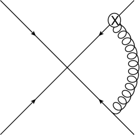
Figure 3: Counterterm graph for the mushroom diagram of figure 2$(a)$, where $\otimes$ denotes the counterterm for the gluon emission vertex from the Wilson line.

Summing up the results of the non-renormalized graph, eq. (3.12), plus the counterterm graph, eq. (3.13), and using the basis functions of eq. (2.50), one finds for the coefficient of the double pole

$$\mathcal{F}_{a,\,{\rm ren.}}^{(2,-2)} =\mathcal{F}_{a}^{(2,-2)}+\mathcal{F}_{a}^{(2,-2)\,{\rm CT}}=-\frac{1}{4}\left(\frac{g_{s}^{2}}{8\pi^{2}}\right)^{2}r(\alpha_{12})M_{0,0,0}(\alpha_{12}),$$ (3.14)

and for the single pole

$$\mathcal{F}_{a,\,{\rm ren.}}^{(2,-1)}=\mathcal{F}_{a}^{(2,-1)}+\mathcal{F}_{a}^{(2,-1)\,{\rm CT}} =-\frac{1}{4}\left(\frac{g_{s}^{2}}{8\pi^{2}}\right)^{2}r(\alpha_{12})\left[M_{1,0,0}(\alpha_{12})-2M_{0,0,0}(\alpha_{12})\right]\,,$$ (3.15)

where the explicit expressions for $M_{0,0,0}$ and $M_{1,0,0}$ can be found in appendix B. We stress that while the latter result can neatly be written in terms of basis functions, the non-renormalized kinematic function $\mathcal{F}_{a}^{(2,-1)}$ cannot. This is a general feature. We also point out that the dependence on $\ln(\mu^{2}/m^{2})$ has cancelled in the coefficient of the $1/\epsilon$ pole between eq. (3.12) and eq. (3.13), as it must do given that the infrared regulator $m$ cannot appear in the final result for the soft anomalous dimension.

We can now use these results to calculate the contribution of the entire web of figure 2 to the soft anomalous dimension. We first need the web mixing matrix, that describes how to combine the kinematic and colour parts of individual diagrams in the web. Using the algorithm of ref. [55] (reviewed here in appendix D) for the (3,1) web, we find that the combination of eq. (2.14) evaluates to

$$W_{(3,1)}=\frac{1}{2}\left(\begin{array}[]{ccc}{\cal F}(a)&{\cal F}(b)&{\cal F}(c)\end{array}\right)\left(\begin{array}[]{rrr}2&-1&-1\\ 0&1&-1\\ 0&-1&1\end{array}\right)\left(\begin{array}[]{c}C(a)\\ C(b)\\ C(c)\end{array}\right).$$ (3.16)

We have already given the colour factor of diagram $(a)$ in eq. (3.6). The colour factors of the other two diagrams are

$$C(b) =T_{1}^{b}\,T_{1}^{b}\,T_{1}^{a}\,T_{2}^{a}=C_{R_{1}}T_{1}^{a}T_{2}^{a};$$

$$C(c) =T_{1}^{a}\,T_{1}^{b}\,T_{1}^{b}\,T_{2}^{a}=C(b),$$ (3.17)

where as usual $C_{R_{i}}$ denotes a quadratic Casimir in the representation of line $i$. The fact that the colour factors of diagrams ($b$) and ($c$) are equal, and evaluate to the $C_{R_{1}}$-dependent part of diagram $(a)$, means that eq. (3.16) simplifies considerably to

$$W_{(3,1)}=\frac{1}{2}{\cal F}(a)\left[2C(a)-C(b)-C(c)\right]=-\frac{1}{2}N_{c}(T_{1}\cdot T_{2}){\cal F}(a)\,.$$ (3.18)

The single pole of eq. (3.18) contributes to the two-loop soft anomalous dimension $\Gamma^{(2)}$, as prescribed by eq. (2.1). The commutator term that converts the web into a subtracted web is zero, given that the only lower-order subwebs in the (3,1) web are the self-energy bubble, and a single gluon exchange between the two Wilson lines. As discussed in section 3.1, the colour factor of the self-energy graph is a constant, and thus commutes with all other webs. We can then immediately identify the contribution of (3,1) webs to the two-loop soft anomalous dimension to be

$$\Gamma^{(2)}\Big{|}_{(3,1)}=-4w_{(3,1)}^{(2,-1)}=\sum_{i\neq j}\frac{1}{2}N_{c}(T_{i}\cdot T_{j})\left(\frac{1}{2\pi}\right)^{2}r(\alpha_{ij})\Big{[}2M_{0,0,0}(\alpha_{ij})-M_{1,0,0}(\alpha_{ij})\Big{]},$$ (3.19)

where we have used eq. (3.15), and summed over all pairs of Wilson lines $i$ and $j$ (n.b. each pair occurs twice in the sum, given that the boomerang gluon can be on line $i$ or $j$). The result in eq. (3.19) agrees with previous calculations, in particular it can be checked that it reproduces the (non-Abelian part of the) coefficient of the single-logarithmic term in eq. (42) of ref. [7] upon relating the kinematic variables according to $\mathrm{\gamma}=\ln\alpha$.

To summarise, we have shown in detail how to adapt the exponential regulator of eq. (2.2) to the calculation of boomerang webs. We do it by simply removing this regulator for boomerang gluons, so as to be able to cleanly isolate ultraviolet singularities associated with the cusp, from those that have to do with the renormalization of the coupling. The regularization of the non-boomerang gluons at large distances is sufficient to render diagrams in which they are straddled by non-regularized boomerang gluons infrared-finite. A simplification in the calculation of the (3,1) web was that self-energy diagrams (i.e. diagrams $(b)$ and $(c)$ in figure 2) do not contribute to the final expression for the web, despite the fact that their individual colour factors and kinematic parts are non-zero. In fact, this property persists at higher perturbative orders, and thus greatly streamlines the calculation of boomerang webs at three loops and beyond. We present a proof of this result in section 4, so that we can reliably use it throughout the remainder of the paper.

Considering the contribution of the (3,1) web to the soft anomalous dimension in eq. (3.19), we note that the general structure is similar to that of non-boomerang MGEWs analysed in refs. [44, 45], namely an overall rational function $r(\alpha_{ij})$ associated with the non-boomerang gluon, multiplying a pure transcendental function. Furthermore, the latter may still be written in terms of the basis functions defined in eq. (2.50). However, while non-boomerang MGEWs are characterized by a uniform maximal weight (that is the contribution to the anomalous dimension at $n$ loops is of weight $2n-1$) the (3,1) web displays mixed (non-uniform) non-maximal weight: eq. (3.19) features both weight 2 ($M_{1,0,0}$) and weight 1 ($M_{0,0,0}$) contributions. The origin of this weightdrop can be traced back to the integration over the boomerang gluon yielding the factor $1/(1-2\epsilon)$ in eq. (3.12) (cf. a similar factor appearing in the self-energy diagram of eq. (3.4)). This weightdrop is a general characteristic of boomerang webs and is discussed further below in section 3.3 and in the context of the three-loop examples in section 5.

3.3 Kinematic factors of boomerang webs

In section 2.4, we discussed the general procedure for calculating MEGWs of refs. [44, 45], where an explicit assumption of this method was that each gluon propagates between different Wilson lines. The latter is no longer true once boomerang gluons are present, and the results of the previous two sections can be used to guide us towards a suitable generalisation of the MGEW integrand, which encompasses the new feature. Given a MGEW with $n$ gluon exchanges in total, out of which $b$ are boomerang gluons, we must modify eq. (2.4) as follows:

$$\begin{split}{\cal F}^{(n)}\left(D\right)&=\,\left(\frac{1}{2}\,g_{s}^{2}\bar{\mu}^{2\epsilon}\,\frac{\Gamma(1-\epsilon)}{4\pi^{2-\epsilon}}\right)^{n}\,\prod_{k=1}^{n-b}\Bigg{[}\int_{0}^{\infty}d\lambda_{k}\,\lambda_{k}^{-1+2\epsilon}\,{\rm e}^{-i(m-i\varepsilon)\lambda_{k}}\\ &\qquad\times\,\,\int_{0}^{1}dx_{k}\,\gamma_{k}\,\Big{(}-x_{k}^{2}-(1-x_{k})^{2}+\gamma_{k}\,x_{k}(1-x_{k})+i\varepsilon\Big{)}^{-1+\epsilon}\Bigg{]}\\ &\times\,\,\prod_{l=n-b+1}^{n}\Bigg{[}\int_{0}^{\infty}d\lambda_{l}\,\lambda_{l}^{-1+2\epsilon}\int_{0}^{1}dx_{l}\,2\left[-(2x_{l}-1)^{2}+i\varepsilon\right]^{\epsilon-1}\,\,\Bigg{]}\Theta_{D}\big{[}\left\{x_{i},\lambda_{i}\right\}\big{]}\,.\end{split}$$ (3.20)

The first two lines correspond to the $n-b$ non-boomerang gluon exchanges, and follow a similar format to eq. (2.4), including the presence of the exponential regulator. The third line contains the integrations associated with the $b$ boomerang gluons, where the exponential regulator has been removed as discussed in the previous section. Furthermore, the propagator function in each $x_{l}$ integral has been replaced with its appropriate form for $\gamma_{l}\rightarrow 2$. Finally, the third line also contains the Heaviside functions implementing the gluon orderings along the Wilson lines for a given diagram, which may potentially involve both the boomerang, and non-boomerang, gluons.

While the convergence of the integrations over the distance parameters $\lambda_{k}$ for the non-boomerang gluons ($k\leq n-b$) is clearly guaranteed by the regulating exponentials, it is less obvious from eq. (3.20) that also those for the boomerang gluons, that is, $\lambda_{l}$ for all $n-b+1\leq l\leq n$, are regulated. Closer inspection of these integrals reveals that they are in fact regulated in all cases of interest, namely so long as Wilson-line self-energy subdiagrams are excluded. One way to see this is to observe that each boomerang gluon then necessarily straddles at least one other gluon emission, be it another boomerang gluon or a non-boomerang one. Furthermore, each boomerang cluster (a subdiagram involving one or more boomerang gluons) limits the upper integration limit over some non-boomerang gluon along the Wilson line, and it also limits the lower integration limit of some (possibly another) non-boomerang gluon along the same line. Upon performing the integration over all boomerang $\lambda_{l}$ parameters first, one then necessarily hits both an upper and a lower limit of integration due to the Heaviside functions $\Theta_{D}\big{[}\left\{x_{i},\lambda_{i}\right\}\big{]}$, linking the distance parameters $\lambda_{l}$ for the boomerang gluons to those of the non-boomerang ones, $\lambda_{k}$ for $k\leq n-b$, which are in turn regularised by the exponentials. This mechanism was seen already in the context of the (3,1) web above (see in particular eq. (3.10)); we now see that it is completely general, and we will give further examples at three loops in section 5.

It is convenient to rewrite eq. (3.20) so as to expose the general properties of boomerang webs. To this end, we may introduce variable transformations analogous to eq. (2.34):

$$\lambda_{k}=(1-y_{k-1})\prod_{p=k}^{n-b}y_{p},\quad k=1,\ldots,n-b,\quad y_{0}=0,$$ (3.21)

where the product now includes the non-boomerang gluons only. One may also decouple the distance parameters $\{\lambda_{l}\}$ of the boomerang gluons from their non-boomerang counterparts by defining

$$\lambda_{l}=y_{n-b}\,\tilde{\lambda}_{l},$$ (3.22)

after which one may perform the $y_{n-b}$ integral in eq. (3.20) to obtain

$${\cal F}^{(n)}\left(D\right) =\,\kappa^{n}\,\Gamma(2n\epsilon)\prod_{k=1}^{n-b}\left[\int_{0}^{1}dx_{k}\,\gamma_{k}\,P_{\epsilon}(x_{k},\gamma_{k})\right]\prod_{l=n-b+1}^{n}\left[\int_{\frac{1}{2}}^{1}dx_{l}\,[(2x_{l}-1)^{2}]^{\epsilon-1}\right]\,\phi_{D}^{(n)}(\{x_{i}\};\epsilon),$$ (3.23)

where the kernel is now defined by

$$\phi_{D}^{(n)}(\{x_{i}\};\epsilon) =2^{b}\prod_{k=1}^{n-b-1}\left[\int_{0}^{1}dy_{k}(1-y_{k})^{-1+2\epsilon}y_{k}^{-1+2k\epsilon}\right]\prod_{l=n-b+1}^{n}\left[\int_{0}^{\infty}d\tilde{\lambda}_{l}\tilde{\lambda}_{l}^{-1+2\epsilon}\right]\Theta_{D}\big{[}\big{\{}x_{i},\tilde{\lambda}_{i},y_{i}\big{\}}\big{]},$$ (3.24)

where the $\tilde{\lambda}_{l}$ integrals are bounded by the Heaviside functions, as explained above.

The general representation of boomerang MGEWs in eq. (3.23) gives us an opportunity to recall some of the general properties of MGEWs [70, 44, 45], and then pinpoint the differences between those containing boomerang gluons and those which do not. Equation (3.23) much like its boomerang-free analogue, eq. (2.35), represents at $n$-loop order an integration over the $2n$ positions of emission and absorption of the $n$ gluons along the Wilson lines. As we have seen in the previous section, these integrals ultimately lead to a result for the subtracted web, that is a contribution to the soft anomalous dimension, taking the form of eq. (2.46), with a rational factor consisting of a factor of $r(\alpha_{ij})$ for each gluon exchange between lines $i$ and $j$, multiplying a pure transcendental function of $\{\alpha_{ij}\}$ with polylogarithmic weight $2n-1$. Equation (2.35) explains the origin of this pure, maximal weight structure: every integral over $y_{k}$ in eq. (2.38) is an integral over a $d\log$ form, with endpoint singularities regularised by $\epsilon>0$. The resulting kernel is therefore a pure function of weight $n-1$, that is, the $\epsilon^{0}$ term in its Laurent expansion is of weight $n-1$, and upon assigning $\epsilon$ weight $-1$, all the terms in the Laurent expansion have the same weight. A similar thing happens at the next stage, when the kernel is integrated with respect to the propagators in eq. (2.35). At this stage the linear denominator is generated by the propagators (see eq. (2.44)), and again, each and every integral over $x_{k}$ results in an increase of one unit in the transcendental weight. This is true for each and every diagram contributing to the web, as well as the commutators entering the subtracted web.

Consider now the analogous structure of the integration in the case of boomerang webs. In eq. (3.24) we see $n-b-1$ integrals over non-boomerang $y_{k}$ variables plus $b$ integrals over boomerang distance scales $\tilde{\lambda}_{l}$. Both are of $d\log$ form, regularized by $\epsilon>0$. Thus, again in total we have $n-1$ integrals each contributing to the weight of $\phi_{D}$. The latter must therefore still be a pure function of weight $n-1$. The differences to non-boomerang webs occur at the next step, when integrating over the kernel in eq. (3.23). First, a factor of $r(\alpha_{ij})$ is only generated by the $n-b$ non-boomerang propagator integrals over $x_{k}$. Second, while each of the latter integrals is a d$\log$ form, regularised by $\epsilon>0$, which therefore increases the weight by one unit, the remaining $b$ integrals over $x_{l}$ take a rather different form:

$$\int_{\frac{1}{2}}^{1}dx_{l}\,(2x_{l}-1)^{2\epsilon-2}\left(\ldots\right),$$ (3.25)

where the ellipsis denotes the remaining integrand, containing Heaviside functions which may depend on the $\{x_{l}\}$. Such integrals contain a potential divergence associated with the lower limit $x_{l}\rightarrow\frac{1}{2}$. This lower limit of integration corresponds to a local (instantaneous) emission and absorption of the boomerang gluon. Integration over $x_{l}$ in eq. (3.25) produces a factor of

$$\frac{1}{1-2\epsilon}$$ (3.26)

in the final expression for the kinematic function of the corresponding boomerang web diagram.

The pole at $\epsilon=\frac{1}{2}$ represents a linear power divergence. We have already seen such a factor in the self-energy web in eq. (3.4) as well as in the (3,1) web in eq. (3.12). We now see that this is a general feature of boomerang webs. We further note however that there is a qualitative difference between the above two cases. In the self-energy web, the extra factor $\left(\ldots\right)$ in eq. (3.25) is absent, so the integral only exists for $\epsilon>\frac{1}{2}$, and one must first compute it there and then analytically continue the result towards $\epsilon=0$, where it is ultimately expanded. In contrast, in the case of the (3,1) web we can see from eq. (3.11), as already discussed there, that a factor of the form $((1-x)^{-2\epsilon}-x^{-2\epsilon})$ regularises the endpoint singularity at $x=\frac{1}{2}$. It is also clear that the occurrence of this regularising factor is rather general: it appears due to the difference of the two limits of integration over the boomerang gluon $\tilde{\lambda}_{l}$ (this is $\lambda_{1}$ in eq. (3.10)), which must both coincide with the emission point of the other gluon when the boomerang gluon is contracted to a point. This would therefore be the precise form of the factor $\left(\ldots\right)$ in eq. (3.25) whenever a boomerang gluon straddles a single gluon emission. The same considerations apply more generally: whenever a boomerang gluon straddles other emissions at some position $\lambda_{0}$ on the line, both the upper and lower limit of $\tilde{\lambda}_{l}$ coincide with $\lambda_{0}$ when the boomerang gluon is shrunk to a point, namely at $x_{l}\to\frac{1}{2}$. We therefore expect that the factor $\left(\ldots\right)$ multiplying the singularity at $x_{l}=\frac{1}{2}$, would always have a Taylor expansion that begins with a linear term, $(x_{l}-\frac{1}{2})$. This factor regularises the double pole at $x_{l}=\frac{1}{2}$ and renders eq. (3.23) well-defined for any $\epsilon>0$. Of course, poles at $\epsilon\to 0$ will be generated due to end-point singularities. In addition, despite the regularising factor in eq. (3.25), the pole at $\epsilon=\frac{1}{2}$ survives. These features are already present in the example of the (3,1) web in eq. (3.12) and we shall illustrate them in more complex three-loop examples in section 5.

The implications the analysis above, and specifically the presence of the pole at $\epsilon=\frac{1}{2}$, have on the transcendental structure of the kinematic function ${\cal F}^{(n)}$ in eq. (3.23) are clear: instead of increasing the weight by one, as the usual propagator integrals $x_{k}$ in eq. (3.23) do, the $b$ boomerang integrals leave the weight unchanged in as far as the contributions arising from the leading term in the expansion of eq. (3.26) are concerned, and decrease it further in contributions arising from higher-order terms in the $\epsilon$ expansion. This implies, first, that the maximal weight attained in the relevant subtracted web is $2n-1-b$, i.e. a weight drop of one unit for every boomerang web when compared to ordinary MGEWs of the same loop order, and second, that when higher-order terms in the $\epsilon$ expansion are relevant, the subtracted boomerang web would feature mixed (non-uniform) weight. These phenomena were exemplified in the (3,1) web, which features basis functions with weights 2 and 1 (to be contrasted with the maximal weight of 3 of subtracted two-loop MGEWs, see [44, 45]). We will see further examples of this at three loops in section 5 (see a summary in table 2 there).

In order to present explicit results, it is useful to generalise the definition of a subtracted web kernel from eq. (2.46), to the case in which boomerang gluons may be present:

$$F^{(n)}_{W,\,j}\big{(}\alpha_{i}\big{)}=\prod_{k=1}^{n-b}\left[\int_{0}^{1}\,dx_{k}\,p_{0}(x_{k},\alpha_{k})\right]\,{\cal G}^{(n)}_{W,\,j}\Big{(}x_{i},q(x_{i},\alpha_{i})\Big{)}.$$ (3.27)

Here, as above, $b$ is the number of boomerang gluons, and thus the integration only includes propagator functions associated with non-boomerang exchanges. Having discussed the general kinematic properties of boomerang webs, let us now return to the decoupling property of self-energy-type diagrams discussed in the previous section, namely that web diagrams spanning two or more Wilson lines, which contain self-energy subdiagrams (such as those in figures 2$(b)$ and 2$(c)$) do not contribute to the soft anomalous dimension at any order.

4 Decoupling of self-energy diagrams at all orders

Boomerang webs at arbitrary orders in perturbation theory will contain many individual diagrams in which gluons form self-energy-like loops, without straddling one or more gluon emissions that leave the Wilson line. The aim of this section is to formally prove that such graphs do not end up contributing to the web after combination with the web mixing matrix of eq. (2.14). Put another way, if we define the exponentiated colour factors of diagrams in a given web via

$$\tilde{C}(D)=\sum_{D^{\prime}}R_{DD^{\prime}}C(D^{\prime}),$$ (4.1)

where $C(D)$ is the conventional colour factor of diagram $D$, then the exponentiated colour factor of a diagram containing a self-energy loop is zero.

To guide the proof, let us first consider a non-trivial example, namely the (2,4) web of figure 4.

Figure 4: The (2,4) web, where we have assigned replica indices to the gluons in diagrams $(g)$ and $(j)$. Although not drawn here, it is assumed that additional Wilson lines emanate from the Wilson-line cusp.

This has 12 diagrams, 6 of which – diagrams $(g)$ through $(l)$ – involve self-energy bubbles. Let us take two of the graphs, namely $(g)$ and $(j)$, and show that their exponentiated colour factors vanish. To this end, we can perform a replica analysis as in ref. [55] or appendix D, and we have labelled the gluons in the figure with appropriate replica indices $(i,j,k)$. In table 1, we show the possible hierarchies $h$ of replica indices, together with their multiplicities $M_{N}(h)$. We also show, for each diagram $D$, the colour factor of the diagram obtained from ordering the replica indices along the Wilson line (such that larger replica indices are closer to the Wilson-line vertex), labelled by ${\cal R}[D|h]$. The exponentiated colour factors of the two diagrams considered are given by eq. (D.1), and we find

$$\begin{split}\tilde{C}(g)&=\frac{C(g)}{2}-\frac{C(h)}{3}-\frac{C(i)}{6};\\ \tilde{C}(j)&=-\frac{C(g)}{3}-\frac{C(h)}{3}+\frac{2C(i)}{3}+\frac{C(j)}{2}-\frac{C(l)}{2}.\end{split}$$ (4.2)

$h$	${\cal R}[g|h]$	${\cal R}[j|h]$	$M_{N}(h)$	${\cal O}(N)$ part of $M_{N}(h)$
$i=j=k$	$C(g)$	$C(j)$	$N$	1
$i=j<k$	$C(h)$	$C(h)$	$\frac{1}{2}N(N-1)$	$-\frac{1}{2}$
$i=j>k$	$C(g)$	$C(g)$	$\frac{1}{2}N(N-1)$	$-\frac{1}{2}$
$i=k<j$	$C(h)$	$C(h)$	$\frac{1}{2}N(N-1)$	$-\frac{1}{2}$
$i=k>j$	$C(g)$	$C(g)$	$\frac{1}{2}N(N-1)$	$-\frac{1}{2}$
$j=k<i$	$C(g)$	$C(j)$	$\frac{1}{2}N(N-1)$	$-\frac{1}{2}$
$j=k>i$	$C(i)$	$C(l)$	$\frac{1}{2}N(N-1)$	$-\frac{1}{2}$
$i<j<k$	$C(i)$	$C(i)$	$\frac{1}{6}N(N-1)(N-2)$	$\frac{1}{3}$
$i<k<j$	$C(i)$	$C(i)$	$\frac{1}{6}N(N-1)(N-2)$	$\frac{1}{3}$
$j<i<k$	$C(h)$	$C(h)$	$\frac{1}{6}N(N-1)(N-2)$	$\frac{1}{3}$
$j<k<i$	$C(g)$	$C(g)$	$\frac{1}{6}N(N-1)(N-2)$	$\frac{1}{3}$
$k<i<j$	$C(h)$	$C(h)$	$\frac{1}{6}N(N-1)(N-2)$	$\frac{1}{3}$
$k<j<i$	$C(g)$	$C(g)$	$\frac{1}{6}N(N-1)(N-2)$	$\frac{1}{3}$

Table 1: Replica analysis of the (2,4) web of figure 4.

We may now use the fact that a self-energy loop contributes a factor $T_{i}^{a}T_{i}^{a}=C_{R_{i}}$ to the colour factor of any web diagram, which is diagonal in colour space. Thus, graphs which differ only by the placement of a self-energy loop on a given Wilson line have equal colour factors. For the specific web of figure 4, this implies

$$C(g)=C(h)=C(i),\qquad C(j)=C(k)=C(l).$$ (4.3)

Equation (4.2) then immediately implies

$$\tilde{C}(g)=\tilde{C}(j)=0.$$ (4.4)

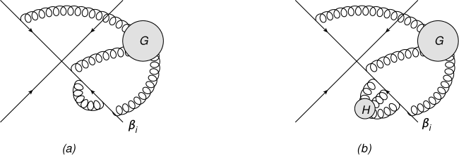
Figure 5: $(a)$ General web diagram containing a self-energy loop, where the rest of the diagram $G$ consists of a number of connected pieces; $(b)$ generalisation to include a non-trivial subdiagram $H$ in place of the self-energy loop.

In the above replica analysis (and as noted in ref. [55]), a hierarchy $h$ containing $r$ distinct replica indices has multiplicity

$${\cal M}_{N}[h(r)]=\left(\begin{array}[]{c}N\\ r\end{array}\right)=\frac{1}{r!}N(N-1)\ldots(N-r+1),$$ (4.5)

and thus contributes the following to the ${\cal O}(N)$ part of the replicated colour factor:

$${\cal M}_{N}[h(r)]\Big{|}_{{\cal O}(N)}=\frac{(-1)^{r-1}}{r}.$$ (4.6)

Now consider a general web diagram $D$ containing a self-energy loop on line $i$, as shown in figure 5($a$). Here $G$ is the rest of the graph, which must contain at least one gluon connecting to another Wilson line, and may potentially consist of a number of connected pieces. Let us assume that a hierarchy of replica indices has already been assigned to $G$, and that this has $r$ distinct indices. For a given hierarchy $h$ of replica indices for the entire diagram, we must reorder those gluons on line $i$ whose replica numbers differ. However, this reordering can never make the self-energy loop straddle another gluon emission: both endpoints of the boomerang gluon have the same replica number, and so cannot appear on opposite sides of another gluon attachment whose replica number is different. The most that can happen is that the self-energy loop as a whole is shifted along the line. According to eq. (D.1), for each hierarchy $h$, we must record the colour factor ${\cal R}[D|h]$ obtained after the reordering. The contribution to this colour factor from the self-energy loop is $C_{R_{i}}$, which is diagonal in colour space. Given that the hierarchy of replica indices for the subgraph $G$ have already been fixed, it follows that for every hierarchy $h$ (including the replica index for the self-energy loop), the reordered colour factor ${\cal R}[D|h]$ is the same, and given by

$${\cal R}[D|h]=C_{R_{i}}{\cal R}[G|h]$$ (4.7)

There are then two possibilities when inserting replica index $i$ of the self-energy loop to give the full hierarchy $h$:

1. The index $i$ is the same as one of the $r$ indices already assigned in $G$. Here the $h$ contributes with a multiplicity factor $(-1)^{r-1}/r$, from eq. (4.6). There are $r$ choices for $i$, so that the contribution to the exponentiated colour factor from all such choices is

   $$r\frac{(-1)^{r-1}}{r}C_{R_{i}}{\cal R}[G|h]=(-1)^{r-1}C_{R_{i}}{\cal R}[G|h],$$ (4.8)

   where we have used eq. (4.7) in eq. (D.1).

2. The index $i$ is distinct from the $r$ indices already ordered in $G$. Now there are $r+1$ distinct replica numbers in total in $h$, so that $h$ has a multiplicity factor $(-1)^{r}/(r+1)$. There are $r+1$ possible placings for the replica index $i$ (i.e. it may be less than or greater than any of the existing $r$ replica numbers), and thus the total contribution to the exponentiated colour factor is

   $$(r+1)\frac{(-1)^{r}}{r+1}C_{R_{i}}{\cal R}[G|h]=(-1)^{r}C_{R_{i}}{\cal R}[G|h].$$ (4.9)

Adding together eqs. (4.8) and (4.9), the total contribution to $\tilde{C}(D)$ from the hierarchy $h$ for subdiagram $G$ is

$$\left((-1)^{r-1}+(-1)^{r}\right)C_{R_{i}}{\cal R}[G|h]=0.$$ (4.10)

The full calculation of $\tilde{C}(D)$ requires a sum over all hierarchies for the full diagram. This is easily rewritten as a sum over all hierarchies, $h$, of $G$ then a sum over all assignments of $i$ for the extra gluon. Each of these sub-sums is zero by eq. (4.10), hence the required result that indeed $\tilde{C}(D)=0$.

To clarify the above proof, we can revisit the replica analysis of the (2,4) web in table 1. Considering first diagram $(g)$, the subdiagram $G$ consists of a ladder of two gluon exchanges between the two active Wilson lines. There are then three possible assignments of replica indices $j$ and $k$ to $G$. If $j=k$ (corresponding to $r=1$ distinct indices), then in assigning a replica index to the self-energy loop one may choose $i=j$ or $i\neq j$. When the index $i$ is the same as $(j,k)$ one obtains the colour factor $C(g)$, with multiplicity factor 1. Alternatively, we may have $i<j$ or $i>j$, giving colour factors $C(i)$ or $C(g)$ respectively, and each with a multiplicity factor of $-1/2$. However, $C(g)=C(i)$, so that the total contribution to the exponentiated colour factor is $C(g)\big{(}1-\frac{1}{2}-\frac{1}{2}\big{)}=0$. A similar analysis can be applied to the other possible hierarchies $j<k$ and $j>k$ for the subdiagram $G$, and also for the second diagram $(j)$ considered in table 1.

As well as the above result for self-energy loops, we can also prove a more general result. Consider replacing the self-energy loop in figure 5$(a)$ with a subdiagram $H$ consisting of more than one connected piece in general, but such that none of its gluon attachments on Wilson line $i$ straddle any gluon emissions not in $H$. Let us again label the complete diagram by $D$, containing the subdiagrams $G$ and $H$, such that $H$ is assumed to only attach to Wilson line $i$, while $G$ involves attachments to $i$ and other Wilson lines. We shall now show that the exponentiated colour factors for such diagrams vanish (a result we will use for three-loop boomerang webs in section 5). Let us assume that $r$ replica indices have been assigned to $G$, and $s$ indices to $H$, where the latter potentially overlap with the indices in $G$.

As in the previous proof, we will split the sum over all replica index hierarchies into a sum over sums, which between them cover all hierarchies. We will then show that each is zero. To do this, we define a sub-hierarchy, $\{\{r\},\{s\}\}$, of a replica hierarchy $h$ to be the separated ordering for $G$ and $H$. This is equivalent to undoing a shuffle. For example, $h=\{r_{1}<s_{1}=r_{2}<s_{2}<r_{3}\}$, has sub-hierarchy $\{\{r_{1}<r_{2}<r_{3}\},\{s_{1}<s_{2}\}\}$. Each $h$ has a unique sub-hierarchy, but many different hierarchies may give the same sub-assignment (e.g. $r_{1}<s_{1}<r_{2}<s_{2}<r_{3}$ gives the same sub-hierarchy as above). We then split the sum in eq. (4.1) according to sub-assignment:

$$\tilde{C}(D)=\sum_{{\rm all}\,h}{\cal M}_{N}[h(r,s)]\Big{|}_{{\cal O}(N)}{\cal R}[D|h]=\sum_{\{\{r\},\{s\}\}}\,\,\sum_{{\rm all}\,h\to\{\{r\},\{s\}\}}{\cal M}_{N}[h(r,s)]\Big{|}_{{\cal O}(N)}\,{\cal R}[D|h]\,,$$ (4.11)

where ${\cal R}[D|h]$ is the colour factor of the diagram obtained from $D$ after hierarchy $h$ is applied.

For a given assignment $\{s\}$ of replica indices to $H$, the subdiagram will split into a number of pieces, each of which has a colour factor proportional to the identity, as we are only considering diagrams where $H$ does not connect to any Wilson line other than $i$ and furthermore does not straddle any gluon in $G$ on line $i$. An example for $H$ is given in figure 6$(a)$, which shows a subgraph on a single Wilson line, consisting of two overlapping self-energy loops. If we assign replica indices such that $i<j$, the graph will split into two separate self-energy loops (figure 6$(b)$), each with colour factor $C_{R_{i}}\mathbb{1}$, which is different to the colour factor of figure 6$(a)$. We use the organisation of the sum in eq. (4.11), to treat the contribution for each hierarchy of $H$ separately, so in this example the hierarchies with $i=j$ are considered separately to those with $i<j$.

Figure 6: $(a)$ Generalised self-energy diagram on a single Wilson line, with replica indices $i$ and $j$; $(b)$ replica ordered version, if $i<j$.

For a fixed assignment of the $r$ replica indices to $G$ and $s$ indices in $H$, different hierarchies of the full set of replicas will potentially reorder the parts of $H$ along the Wilson line, according to the mutual ordering between the indices of $G$ and $H$. However, because both before and after this reordering none of the subdiagrams in $H$ straddle any gluon emissions in $G$ and the colour factor of the subdiagram $H$ (and its subdiagrams if present) are proportional to the identity, it follows that all choices with the same sub-hierarchy $\{\{r\},\{s\}\}$ will lead to a diagram with the same colour factor. We may express this common colour factor as the product ${\cal R}[G|\{r\}]\,{\cal R}[H|\{s\}]$, noting explicitly that it depends on the choice of the $r$ indices in $G$ and $s$ indices in $H$, but not on how they are interleaved.

Combining $H$ and $G$, we will have a total number of indices

$$n=r+s-k,\quad k\in[0,\min(r,s)]$$ (4.12)

where $k$ is the number of indices that overlap (i.e. are set equal) between $G$ and $H$. From eq. (4.6), the overall hierarchy $h$ will contribute with a multiplicity factor

$$\frac{(-1)^{n-1}}{n}=\frac{(-1)^{r+s-k-1}}{r+s-k}.$$

Returning to the expression for the exponentiated colour factor of $D$ in eq. (4.11), we have now found that the inner sum can be written as

$$\sum_{{\rm all}\,h\to\{\{r\},\{s\}\}}{\cal M}_{N}[h(r,s)]\Big{|}_{{\cal O}(N)}\,{\cal R}[D|h]\,=\,{\cal R}[G|\{r\}]\,{\cal R}[H|\{s\}]\sum_{k=0}^{\min(r,s)}N_{r,s,k}\frac{(-1)^{r+s-k-1}}{r+s-k},$$ (4.13)

where $N_{r,s,k}$ is the number of ways of assigning $r$ indices to $G$ and $s$ indices to $H$, with $k$ overlaps. To find this, first note that there are $r+s-k$ distinct indices in total. There are

$$\left(\begin{array}[]{c}r+s-k\\ k\end{array}\right)$$

ways of choosing which indices correspond to the overlapping ones. Of the $r+s-2k$ remaining indices, $(r-k)$ must be chosen to be the remaining indices of $G$ (which has $r$ distinct indices in total), for which there are

$$\left(\begin{array}[]{c}r+s-2k\\ r-k\end{array}\right)$$

possible choices. The remaining $s-k$ indices are then automatically the remaining indices in $H$, and one thus finds

$$N_{r,s,k}=\left(\begin{array}[]{c}r+s-k\\ k\end{array}\right)\left(\begin{array}[]{c}r+s-2k\\ r-k\end{array}\right).$$ (4.14)

Note that $N_{r,s,k}$ is symmetric under $r\leftrightarrow s$ as it must be. From eq. (4.13), the total contribution to the exponentiated colour factor of diagram $D$ is then

$${\cal R}[G|\{r\}]\,{\cal R}[H|\{s\}]\sum_{k=0}^{\min(r,s)}\left(\begin{array}[]{c}r+s-k\\ k\end{array}\right)\left(\begin{array}[]{c}r+s-2k\\ r-k\end{array}\right)\frac{(-1)^{r+s-k-1}}{r+s-k}.$$ (4.15)

To carry out the sum, we may write it as an infinite sum, i.e.,

$$\sum_{k=0}^{\min(r,s)}\left(\begin{array}[]{c}r+s-k\\ k\end{array}\right)\left(\begin{array}[]{c}r+s-2k\\ r-k\end{array}\right)\frac{(-1)^{r+s-k-1}}{r+s-k}$$ (4.20)

$$=\sum_{k=0}^{\min(r,s)}\frac{\Gamma(r+s-k)}{k!\Gamma(r-k+1)\Gamma(s-k+1)}(-1)^{r+s-k-1}$$

$$=\sum_{k=0}^{\infty}\frac{\Gamma(r+s-k)}{k!\Gamma(r-k+1)\Gamma(s-k+1)}(-1)^{r+s-k-1}$$ (4.21)

relying on the fact that for integer $r$ and $s$ the $\Gamma$ functions in the denominator render all terms with $k>\min(r,s)$ identically zero. Next we may consider generic values of $r$ and $s$, for which one may establish that

$$\sum_{k=0}^{\infty}\frac{\Gamma(r+s-k)}{k!\Gamma(r-k+1)\Gamma(s-k+1)}(-1)^{r+s-k-1}=(-1)^{r+s-1}\frac{\sin(\pi r)\sin(\pi s)}{\pi rs\sin(\pi(r+s))}\,,$$ (4.22)

which vanishes in the limit where $r$ and $s$ are positive integers. Thus, each assignment of $r$ replica numbers to the subdiagram $G$ and $s$ replica numbers to the subdiagram $H$ in figure 5$(b)$ leads, upon summing over all hierarchies, to a vanishing contribution to the exponentiated colour factor of the whole diagram. Hence, exponentiated colour factors of diagrams which can be split as in figure 5$(b)$ are zero.

Note that a consistency check of the above proof is that for the case $s=1$, the sum in eq. (4.15) reduces to just two terms, $k=0$ and $k=1$, yielding

$${\cal R}[G|\{r\}]\,{\cal R}[H|\{s\}]\left[(r+1)\frac{(-1)^{r}}{r+1}+r\frac{(-1)^{r-1}}{r}\right]=0,$$

as encountered in the previous proof (cf. eqs. (4.9) and (4.10)).

In summary, we have shown that graphs of the general form of figure 5$(b)$, in which $G$ and $H$ are subdiagrams consisting (in general) of any number of connected pieces, such that $H$ connects to a single line and does not straddle any emission in $G$, have vanishing exponentiated colour factors. Thus, from eq. (2.14), their kinematic parts do not contribute to the logarithm of the soft function, and so do not have to be calculated. For example, we will see in section 5 that of the 15 diagrams in the (5,1) web, only 4 have non-zero exponentiated colour factors. This greatly simplifies the calculation of boomerang webs at three-loop order, which we proceed to do in the following section.

We note that in the above proof we required that $G$ contained at least one gluon connecting to other Wilson lines. This means that the proof above does not apply to webs which consist of multiple boomerang gluons on a single line and nothing else. Indeed these pure self-energy webs are not zero (as we saw with the one-loop self-energy graph in section 3.1) and they do contribute to the soft anomalous dimension. However, because they involve just a single line, these contributions must be entirely independent of kinematic variables and we do not consider them further in this paper.

5 Boomerang webs at three-loop order

In the previous sections, we have prepared the necessary ingredients for the calculation of boomerang MGEWs. We will now focus on the explicit calculation of these webs at the three-loop order. We have seen that at two loops there is a single boomerang web, the (3,1) web. At three loops there are five: two webs involving three Wilson lines, (1,1,4) and (1,2,3) and three webs involving two lines: (3,3), (5,1), and (2,4). As before we shall not assume colour conservation amongst the Wilson lines involved, allowing for a hard interaction vertex involving more lines. The three-line webs are discussed first, in section 5.1, followed by the two-line ones in section 5.2.

5.1 Boomerang webs connecting three Wilson lines

For three-loop webs connecting three lines, the colour basis of eq. (2.26) can be written in the explicit form [58]

$$\begin{split}c_{1}^{[3,3]}&=-f^{ace}f^{bde}T_{1}^{\{a,b\}}T_{2}^{c}T_{3}^{d}=\{T_{1}^{a},T_{1}^{b}\}[T_{2}^{b},T_{2}^{c}][T_{3}^{a},T_{3}^{c}]\\ c_{2}^{[3,3]}&=-f^{cae}f^{bde}T_{1}^{a}T_{2}^{\{b,c\}}T_{3}^{d}=[T_{1}^{a},T_{1}^{b}]\{T_{2}^{b},T_{2}^{c}\}[T_{3}^{a},T_{3}^{c}]\\ c_{3}^{[3,3]}&=-f^{cbe}f^{ade}T_{1}^{a}T_{2}^{b}T_{3}^{\{c,d\}}=[T_{1}^{a},T_{1}^{b}][T_{2}^{b},T_{2}^{c}]\{T_{3}^{a},T_{3}^{c}\}\\ c_{4}^{[3,3]}&=-\frac{1}{2}if^{acd}f^{bef}f^{def}T_{1}^{a}T_{2}^{b}T_{3}^{c}=\frac{1}{2}iN_{c}f^{abc}T_{1}^{a}T_{2}^{b}T_{3}^{c}=[T_{1}^{a},T_{1}^{b}][T_{2}^{b},T_{2}^{c}][T_{3}^{a},T_{3}^{c}]\,.\end{split}$$ (5.1)

For each three-line web, the combinations of kinematic factors accompanying each colour factor have already been derived in ref. [58] using the corresponding mixing matrices. There are two distinct boomerang webs connecting three lines, namely the (1,1,4) web of figure 7, and the (1,2,3) web of figure 8. Let us consider each in turn and compute the relevant integrals.

5.1.1 The jelly-fish (1,1,4) web

The (1,1,4) web consists of twelve distinct diagrams, where six of them (diagrams $(g)$–$(l)$ in figure 7) contain self-energy loops, and are thus irrelevant according to the results of section 4.

Figure 7: The (1,1,4) web.

Following the approach of sections 2 and 3, the kinematic parts of the first six diagrams can be written as

$$\mathcal{F}_{D}(\alpha_{13},\alpha_{23},\epsilon)=\kappa^{3}\Gamma(6\epsilon)\int_{\frac{1}{2}}^{1}\frac{dx}{[(2x-1)^{2}]^{1-\epsilon}}\int_{0}^{1}dydz\,p_{\epsilon}(y,\alpha_{23})\,p_{\epsilon}(z,\alpha_{13})\phi_{D}(x,y,z;\epsilon)\,,$$ (5.2)

where $D\in\{a,b,c,d,e,f\}$, and we present the calculation and results for kernels $\phi_{D}$ in appendix E. The results $\phi_{D}(x,y,z;\epsilon)$ are presented in eqs. (E.7) through (E.12), both as hypergeometric functions depending on $x$, $y$ and $z$, with $\epsilon$ shifting the parameters away from integer values, as well as through an expansion in powers of $\epsilon$. These expressions are useful to illustrate the general discussion around eq. (3.25). Indeed, we observe that each diagram kernel consists of differences between pairs of hypergeometric functions, which vanish at $x=\frac{1}{2}$, providing a linear suppression near the lower endpoint of the $x$ integration in eq. (5.2), such that the double pole associated with the boomerang gluon propagator is regularised, rendering this integral well-defined for small positive $\epsilon$.

We further point out that the suppression of the enpoint singularity at $x=\frac{1}{2}$ can also be easily seen after the $\epsilon$ expansion of the kernel. For diagrams $D\in\{c,d,e,f\}$, where the boomerang gluon straddles a single emission, the $\epsilon$-expanded kernel $\phi_{D}(x,y,z;\epsilon)$ begins with $\sim\frac{1}{\epsilon}\ln((1-x)/x)$ providing linear suppression of the $x=\frac{1}{2}$ singularity. In turn, for diagrams $D\in\{a,b\}$, where the boomerang gluon straddles two emissions, the $\epsilon$-expanded kernel $\phi_{D}(x,y,z;\epsilon)$ begins with $\ln^{2}((1-x)/x)$ providing a quadratic suppression of this singularity.

The exponentiated colour factors for the six diagrams are [58]

$$\tilde{C}(a)=\frac{1}{2}(c_{3}^{[3,3]}-c_{4}^{[3,3]});\ \qquad\tilde{C}(b)=\frac{1}{2}(c_{3}^{[3,3]}+c_{4}^{[3,3]});$$ (5.3)

$$\tilde{C}(c)=\tilde{C}(d)=\frac{1}{2}c_{4}^{[3,3]};\ \qquad\tilde{C}(e)=\tilde{C}(f)=-\frac{1}{2}c_{4}^{[3,3]}\,,$$

where we used the basis of colour factors of eq. (5.1). The complete renormalized web can then be written in this basis as

$$\begin{split}W_{(1,1,4)}=&\,c_{3}^{[3,3]}{\cal F}_{(1,1,4);3}+c_{4}^{[3,3]}\Big{[}{\cal F}_{(1,1,4);4}+{\cal F}_{(1,1,4);4}^{\rm CT}\Big{]},\\ =&\,c_{3}^{[3,3]}\Big{[}\frac{1}{2}\big{(}{\cal F}_{a}+{\cal F}_{b}\big{)}\Big{]}+c_{4}^{[3,3]}\Big{[}\frac{1}{2}\big{(}-{\cal F}_{a}+{\cal F}_{b}+{\cal F}_{c}+{\cal F}_{d}-{\cal F}_{e}-{\cal F}_{f}\big{)}\\ &\qquad\qquad\qquad\qquad\qquad\qquad\qquad+\frac{1}{2}\big{(}{\cal F}_{c}^{\rm CT}+{\cal F}_{d}^{\rm CT}-{\cal F}_{e}^{\rm CT}-{\cal F}_{f}^{\rm CT}\big{)}\Big{]},\end{split}$$ (5.4)

where ${\cal F}_{D}^{\text{CT}}$ is the counterterm contribution associated with the renormalization of the gluon emission vertex in diagram $D$, analogous to eq. (3.13) for the (3,1) web. Note that the counterterm contributions enter with the same coefficient as the diagram they renormalize, thus removing any singularities associated with the shrinking of boomerang gluon loops to a point. As is implied from eq. (5.4), counterterm graphs are not required for diagrams $(a)$ and $(b)$ in figure 7: such a counterterm would correspond to the renormalization of a two-gluon emission vertex coupling to the Wilson line, which is not required.

Using the integrals of eq. (5.2) we immediately find the results for the kinematic functions ${\cal F}_{(1,1,4);3}$ and ${\cal F}_{(1,1,4);4}$ defined by the combinations of contributions from individual diagrams in eq. (5.4); these two are given respectively by eqs. (E.15) and (E). In turn, each of the counterterm contributions entering ${\cal F}_{(1,1,4);4}^{\text{CT}}$ consists of the factor $Z_{v}^{(1)}$ of eq. (C.4) multiplying a lower order graph, obtained by shrinking the boomerang gluon to a point. For each of the diagrams $(c)$–$(f)$ in figure 7, the lower-order diagram will be one of the members of the (1,1,2) web of figure 18, after relabelling of the Wilson lines. Indeed, the combination of graphs appearing in eq. (5.4) is precisely such as to construct the combination of kinematic factors found in the (1,1,2) web (see ref. [55]) and we may thus write

$$\begin{split}{\cal F}_{(1,1,4);4}^{\text{CT}}&(\alpha_{13},\alpha_{23},\mu^{2}/m^{2},\epsilon)=-Z_{v}^{(1)}{\cal F}_{(1,1,2)}^{(2)}(\alpha_{13},\alpha_{23})\\ =&-\frac{1}{2}\left(\frac{g_{s}^{2}}{8\pi^{2}}\right)^{3}\int_{0}^{1}dydz\,p_{0}(y,\alpha_{23})p_{0}(z,\alpha_{12})\Bigg{\{}\frac{1}{\epsilon^{2}}\ln\left(\frac{z}{y}\right)+\frac{1}{\epsilon}\bigg{[}2\text{Li}_{2}\left(-\frac{z}{y}\right)\\ &\quad-2\text{Li}_{2}\left(-\frac{y}{z}\right)+\ln\left(\frac{z}{y}\right)\left(\ln\left(q(y,\alpha_{23})q(z,\alpha_{13})\right)+2\ln\left(\frac{\mu^{2}}{m^{2}}\right)\right)\bigg{]}+\mathcal{O}(\epsilon^{0})\Bigg{\}},\end{split}$$ (5.5)

using eqs. (A.2) and (C.4).

To obtain the renormalized kinematic function multiplying $c_{4}^{[3,3]}$ in (5.4) we now sum up the unrenormalised function of eq. (E) and the counterterm contribution of eq. (5.5), obtaining

$$\begin{split}&{\cal F}_{(1,1,4);4}(\alpha_{13},\alpha_{23},\mu^{2}/m^{2},\epsilon)+{\cal F}_{(1,1,4);4}^{\rm CT}(\alpha_{13},\alpha_{23},\mu^{2}/m^{2},\epsilon)\\ =&\left(\frac{g_{s}^{2}}{8\pi^{2}}\right)^{3}\frac{1}{8}\int_{0}^{1}dydz\,p_{0}(y,\alpha_{23})p_{0}(z,\alpha_{12})\,\ln\left(\frac{z}{y}\right)\\ &\quad\Bigg{\{}-\frac{1}{\epsilon^{2}}+\frac{1}{\epsilon}\left[6+3\ln\left(yz\right)-\ln\left(q(y,\alpha_{23})q(z,\alpha_{13})\right)+\ln\left(\frac{\mu^{2}}{m^{2}}\right)\right]+\mathcal{O}(\epsilon^{0})\Bigg{\}},\end{split}$$ (5.6)

where we note the cancellation of all dilogarithms at ${\cal O}(1/\epsilon)$. With this we have completed the computation of all ingredients in the renormalized $(1,1,4)$ web of eq. (5.4).

For the contribution of this web to the soft anomalous dimension, we must combine eq. (5.4) with the commutator contributions appearing in eq. (2.1), to form the subtracted web $\overline{w}_{(1,1,4)}$ as follows:

$$\overline{w}_{(1,1,4)}^{(3,-1)}=w_{(1,1,4)}^{(3,-1)}+\frac{1}{2}\left[w^{(2,-2)},w^{(1,1)}\right]-\frac{1}{2}\left[w^{(1,0)},w^{(2,-1)}\right]-\frac{1}{2}\left[w^{(2,0)},w^{(1,-1)}\right].$$ (5.7)

Note that, as always, all $w^{(n,k)}$ entering this expression are defined including the counterterms associated with the renormalization of the gluon emission of the Wilson line.

The two lower-order webs which occur in the (1,1,4) web are the single gluon exchange web and the (3,1) web, where the latter has been calculated in section 3. The commutators of these do not yield anything proportional to the colour factor $c_{3}^{[3,3]}$. They do give a contribution to the colour factor $c_{4}^{[3,3]}$, with the kinematic function

$$\begin{split}&{\cal F}_{(1,1,4);4}^{\text{Comm}}(\alpha_{13},\alpha_{23},\mu^{2}/m^{2},\epsilon)\\ &=\frac{1}{2}\left[{\cal F}^{(2,-2)}_{(3,1)}(\alpha_{23}){\cal F}^{(1,1)}(\alpha_{13})-{\cal F}^{(2,-2)}_{(3,1)}(\alpha_{13}){\cal F}^{(1,1)}(\alpha_{23})+{\cal F}^{(2,-1)}_{(3,1)}(\alpha_{23}){\cal F}^{(1,0)}(\alpha_{13})\right.\\ &\qquad\left.-{\cal F}^{(2,-1)}_{(3,1)}(\alpha_{13}){\cal F}^{(1,0)}(\alpha_{23})-{\cal F}^{(2,0)}_{(3,1)}(\alpha_{23}){\cal F}^{(1,-1)}(\alpha_{13})+{\cal F}^{(2,0)}_{(3,1)}(\alpha_{13}){\cal F}^{(1,-1)}(\alpha_{23})\right]\\ &=\frac{1}{8\epsilon}\left(\frac{g_{s}^{2}}{8\pi^{2}}\right)^{3}\int_{0}^{1}dydz\,p_{0}(y,\alpha_{23})p_{0}(z,\alpha_{13})\Bigg{\{}\frac{1}{2}\ln^{2}q(z,\alpha_{13})-\frac{1}{2}\ln^{2}q(y,\alpha_{23})\\ &\qquad\qquad+(2+\ln(yz))\left(\ln q(y,\alpha_{23})-\ln q(z,\alpha_{13})-\ln\left(\frac{z}{y}\right)\right)-\ln\left(\frac{z}{y}\right)\ln\left(\frac{\mu^{2}}{m^{2}}\right)\Bigg{\}}.\end{split}$$ (5.8)

Note that similarly to eq. (5.6) this result is manifestly antisymmetric under the interchange of $\alpha_{23}$ and $\alpha_{13}$. This permutation symmetry is of course consistent with Bose symmetry and the fact that the colour factor $c_{4}^{[3,3]}$ in (5.1) is antisymmetric.

Similarly to eqs. (2.41, 2.46) we can write the final result for the (1,1,4) subtracted web in terms of integrals over subtracted web kernels. Specifically, we define

$$F^{(3)}_{(1,1,4);i}(\alpha_{13},\alpha_{23},\epsilon)=\int_{0}^{1}dx_{1}dx_{2}\,p_{0}(x_{1},\alpha_{13})p_{0}(x_{2},\alpha_{23})\,{\cal G}_{(1,1,4);i}^{(3)}(x_{1},x_{2},\alpha_{13},\alpha_{23})$$ (5.9)

for $i=3,4$. After adjusting for normalisation, we find ${\cal G}_{(1,1,4);3}^{(3)}$ from eq. (E.15) and ${\cal G}_{(1,1,4);4}^{(3)}$ from the sum of the $\epsilon^{-1}$ pole in eq. (5.6) and eq. (5.8):

$${\cal G}_{(1,1,4);3}^{(3)}(x_{1},x_{2},\alpha_{13},\alpha_{23}) =-\frac{4\pi^{2}}{9};$$

$${\cal G}_{(1,1,4);4}^{(3)}(x_{1},x_{2},\alpha_{13},\alpha_{23}) =\frac{1}{2}\left[4\ln\left(\frac{q(x_{2},\alpha_{23})}{x_{2}^{2}}\right)-4\ln\left(\frac{q(x_{1},\alpha_{13})}{x_{1}^{2}}\right)\right.$$ (5.10)

$$\qquad\qquad\left.-\ln^{2}\left(\frac{q(x_{2},\alpha_{23})}{x_{2}^{2}}\right)+\ln^{2}\left(\frac{q(x_{1},\alpha_{13})}{x_{1}^{2}}\right)\right].$$

Again, the antisymmetry under the interchange of $\alpha_{23}$ and $\alpha_{13}$ is manifest. The $\ln(\mu^{2}/m^{2})$ terms have cancelled in the $1/\epsilon$ pole, as they must do to ensure that the soft anomalous dimension does not depend on the regulator $m$. Carrying out the remaining integrals, we obtain the kinematic factors for the subtracted web (defined as in eq. (2.46)):

$$F^{(3)}_{(1,1,4);3}(\alpha_{13},\alpha_{23}) =-\frac{4\pi^{2}}{9}r(\alpha_{13})r(\alpha_{23})M_{0,0,0}(\alpha_{13})M_{0,0,0}(\alpha_{23});$$

$$F^{(3)}_{(1,1,4);4}(\alpha_{13},\alpha_{23}) =\frac{1}{2}r(\alpha_{13})r(\alpha_{23})\Big{[}4M_{1,0,0}(\alpha_{23})M_{0,0,0}(\alpha_{13})-4M_{1,0,0}(\alpha_{13})M_{0,0,0}(\alpha_{23})$$

$$\quad-M_{2,0,0}(\alpha_{23})M_{0,0,0}(\alpha_{13})+M_{2,0,0}(\alpha_{13})M_{0,0,0}(\alpha_{23})\Big{]}\,,$$ (5.11)

where the $M_{k,l,n}(\alpha_{ij})$ are defined in eq. (2.50). Explicit expressions for these functions and their symbols are summarised in appendix B. Note that the first result in eq. (5.11) contains an overall factor of $\pi^{2}$, which itself has a non-zero transcendental weight. It is then natural to ask whether one can rewrite this result to be purely in terms of (products of) our basis functions with purely rational coefficients. That this is indeed the case can be seen by noting that (see appendix B)

$$\frac{4\pi^{2}}{3}M_{0,0,0}(\alpha)=4M_{0,2,0}(\alpha)-M_{0,0,2}(\alpha).$$ (5.12)

Thus, one may write

$$F_{(1,1,4);3}^{(3)} =-\frac{1}{6}r(\alpha_{13})r(\alpha_{23})\Big{[}\Big{(}4M_{0,2,0}(\alpha_{13})-M_{0,0,2}(\alpha_{13})\Big{)}M_{0,0,0}(\alpha_{23})$$

$$\quad+M_{0,0,0}(\alpha_{13})\Big{(}4M_{0,2,0}(\alpha_{23})-M_{0,0,2}(\alpha_{23})\Big{)}\Big{]},$$ (5.13)

where we have made the symmetry of the web under the interchange of lines 1 and 2 manifest. We see once again the same general pattern previously seen in MGEWs and in the (3,1) web in section 3.2: the subtracted web kinematic function takes the form of a rational function consisting of one factor of $r(\alpha_{ij})$ for each gluon which connects distinct Wilson lines $i$ and $j$, multiplied by a pure transcendental function. The latter consists of a sum of products of polylogarithmic functions of individual $\alpha_{ij}$. The latter are again drawn from the basis of $M_{k,l,n}(\alpha_{ij})$ proposed in ref. [45].

We further note that as in the case of the (3,1) web – and in contrast to non-boomerang MGEWs – the polylogarithmic function in eq. (5.11) is of mixed, non-maximal weight, here weight 3 and weight 4, while the soft anomalous dimension at three loops receives contributions starting at weight 5. We will see a similar mixed, non-maximal weight structure across all boomerang webs.

5.1.2 The (1,2,3) web

Next, we consider the (1,2,3) web of figure 8, consisting of six diagrams. However, four of these (diagrams $(c)$–$(f)$) contain self-energy loops, and thus do not contribute to the logarithm of the soft function, using the results of section 4.

Figure 8: The (1,2,3) web.

From ref. [58], the exponentiated colour factors of diagrams $(a)$ and $(b)$ are

$$\tilde{C}(a)=-\frac{1}{2}c_{4}^{[3,3]}\quad{\rm and}\quad\tilde{C}(b)=\frac{1}{2}c_{4}^{[3,3]}.$$ (5.14)

Therefore, the renormalized web is given by

$$\begin{split}W_{(1,2,3)}&=\,c_{4}^{[3,3]}\Big{[}{\cal F}_{(1,2,3);4}+{\cal F}_{(1,2,3);4}^{\rm CT}\Big{]}\\ &=\,c_{4}^{[3,3]}\Big{[}-\frac{1}{2}\big{(}{\cal F}_{a}-{\cal F}_{b}\big{)}-\frac{1}{2}\big{(}{\cal F}_{a}^{\rm CT}-{\cal F}_{b}^{\rm CT}\big{)}\Big{]}.\end{split}$$ (5.15)

Using similar methods to the (1,1,4) web, we find that the kinematic parts of these diagrams are given by

$$\mathcal{F}_{D}(\alpha_{12},\alpha_{23},\epsilon)=\kappa^{3}\Gamma(6\epsilon)\frac{1}{\epsilon}\frac{1}{1-2\epsilon}\int_{0}^{1}dydz\,y^{2\epsilon}p_{\epsilon}(y,\alpha_{23})p_{\epsilon}(z,\alpha_{12})\phi_{D}(y,z),$$ (5.16)

where

$$\begin{split}\phi_{a}(y,z)&=\frac{1}{2\epsilon}\left(\frac{1-y}{z}\right)^{2\epsilon}{{}_{2}}F_{1}\left(6\epsilon,2\epsilon;1+2\epsilon;-\frac{1-y}{z}\right)\\ &=\frac{1}{2\epsilon}+\ln\left(\frac{1-y}{z}\right)+\left\{\ln^{2}\left(\frac{1-y}{z}\right)+6\text{Li}_{2}\left(-\frac{1-y}{z}\right)\right\}\epsilon+\mathcal{O}(\epsilon^{2});\\ \phi_{b}(y,z)&=\frac{1}{4\epsilon}\left(\frac{z}{1-y}\right)^{4\epsilon}{{}_{2}}F_{1}\left(6\epsilon,4\epsilon;1+4\epsilon;-\frac{z}{1-y}\right)\\ &=\frac{1}{4\epsilon}+\ln\left(\frac{z}{1-y}\right)+\left\{2\ln^{2}\left(\frac{z}{1-y}\right)+6\text{Li}_{2}\left(-\frac{z}{1-y}\right)\right\}\epsilon+\mathcal{O}(\epsilon^{2})\,,\end{split}$$ (5.17)

and where ${{}_{2}}F_{1}(a,b;c;z)$ is the Gauss hypergeometric function. The integrals corresponding to the boomerang gluon have already been performed here, generating the pole at $\epsilon=\frac{1}{2}$ in eq. (5.16). To these, we must add the ultraviolet counterterm graphs, ${\cal F}_{a}^{\rm CT}$ and ${\cal F}_{b}^{\rm CT}$, associated with renormalization of the gluon emission vertex in graphs $(a)$ and $(b)$ respectively. As for the (1,1,4) web, the counterterms construct the (1,1,2) web of eq. (A.2), where line $2$ in figure 8 is the one having two gluon attachments. The resulting counterterm contribution in eq. (5.15) is

$$\begin{split}{\cal F}_{(1,2,3);4}^{\rm CT}&(\alpha_{12},\alpha_{23},\mu^{2}/m^{2},\epsilon)=-\frac{1}{2}Z_{v}^{(1)}{\cal F}^{(2)}_{(1,1,2)}(\alpha_{12},\alpha_{23},\epsilon)\\ =&\ \frac{1}{4}\left(\frac{g_{s}^{2}}{8\pi^{2}}\right)^{3}\int_{0}^{1}dydz\,p_{0}(y,\alpha_{23})p_{0}(z,\alpha_{12})\Bigg{\{}\frac{1}{\epsilon^{2}}\ln\left(\frac{z}{y}\right)+\frac{1}{\epsilon}\Bigg{[}2\text{Li}_{2}\left(-\frac{z}{y}\right)\\ &-2\text{Li}_{2}\left(-\frac{y}{z}\right)+\ln\left(\frac{z}{y}\right)\left(\ln\left(q(y,\alpha_{23})q(z,\alpha_{12})\right)+2\ln\left(\frac{\mu^{2}}{m^{2}}\right)\right)\Bigg{]}+\mathcal{O}(\epsilon^{0})\Bigg{\}},\end{split}$$ (5.18)

using eq. (C.4). Combining this with the results from eq. (5.17) gives the final result for the kinematic function multiplying $c_{4}^{[3,3]}$ in the renormalized (1,2,3) web in eq. (5.15) to be

$$\begin{split}&{\cal F}_{(1,2,3);4}(\alpha_{12},\alpha_{23},\mu^{2}/m^{2},\epsilon)+{\cal F}_{(1,2,3);4}^{\rm CT}(\alpha_{12},\alpha_{23},\mu^{2}/m^{2},\epsilon)\\ =&\ \frac{1}{48}\left(\frac{g_{s}^{2}}{8\pi^{2}}\right)^{3}\int_{0}^{1}dydz\,p_{0}(y,\alpha_{23})p_{0}(z,\alpha_{12})\,\Bigg{\{}\frac{1}{\epsilon^{3}}\\ &\quad+\frac{1}{\epsilon^{2}}\left[2+3\ln\left(\frac{\mu^{2}}{m^{2}}\right)+\ln\left(q(y,\alpha_{23})q(z,\alpha_{12})\right]-2\ln(y)+4\ln(z)\right]\\ &\quad+\frac{1}{2\epsilon}\left[8+\frac{13\pi^{2}}{2}+40\ln(y)-32\ln(z)+\ln^{2}\left(q(y,\alpha_{23})q(z,\alpha_{12})\right)-4\ln^{2}(y)\right.\\ &\qquad+32\ln(y)\ln(1-y)-16\ln(y)\ln(z)-8\ln^{2}(z)\\ &\qquad+4\ln\left(q(y,\alpha_{23})q(z,\alpha_{12})\right)\left(1-\ln(y)+2\ln(z)\right)\\ &\qquad\left.+3\ln\left(\frac{\mu^{2}}{m^{2}}\right)\left(4+2\ln\left(q(y,\alpha_{23})q(z,\alpha_{12})\right)+4\ln(y)+3\ln\left(\frac{\mu^{2}}{m^{2}}\right)\right)\right]+{\cal O}(\epsilon^{0}).\end{split}$$ (5.19)

Once again the dilogarithms have cancelled to this order in $\epsilon$ in the renormalised result.

In order to obtain the corresponding contribution of this web to the soft anomalous dimension, the $(1,2,3)$ subtracted web, we must now add to eq. (5.19) the commutator contributions involving lower-order webs. As is clear from figure 8, the relevant lower-order webs include the single gluon exchange (one-loop) diagram, and the (3,1) web of figure 2 and we find

$$\overline{w}_{(1,2,3)}^{(3,-1)}=w_{(1,2,3)}^{(3,-1)}\,+\,c_{4}^{[3,3]}{\cal F}^{\rm Comm}_{(1,2,3);4}(\alpha_{12},\alpha_{23},\mu^{2}/m^{2},\epsilon),$$ (5.20)

where

$$\begin{split}{\cal F}^{\rm Comm}_{(1,2,3);4}&(\alpha_{12},\alpha_{23},\mu^{2}/m^{2},\epsilon)\\ =\,&\frac{1}{2\epsilon}\left(-{\cal F}^{(1,1)}(\alpha_{12}){\cal F}^{(2,-2)}_{(1,3)}(\alpha_{23})-{\cal F}^{(1,0)}(\alpha_{12}){\cal F}^{(2,-1)}_{(1,3)}(\alpha_{23})+{\cal F}^{(2,0)}_{(1,3)}(\alpha_{23}){\cal F}^{(1,-1)}(\alpha_{12})\right)\\ =\,&-\frac{1}{32\epsilon}\left(\frac{g_{s}^{2}}{8\pi^{2}}\right)^{3}\int_{0}^{1}dydz\,p_{0}(y,\alpha_{23})p_{0}(z,\alpha_{12})\\ &\quad\times\bigg{[}8+\frac{13\pi^{2}}{6}+4\ln(q(y,\alpha_{23}))-4\ln(q(z,\alpha_{12}))-\ln^{2}(q(y,\alpha_{23}))\\ &\qquad\qquad+\ln^{2}(q(z,\alpha_{12}))+2\ln(q(y,\alpha_{23}))\ln(q(z,\alpha_{12}))+8\ln(y)+4\ln^{2}(y)\\ &\qquad\qquad+4\ln(q(y,\alpha_{23}))\ln(y)-4\ln(q(z,\alpha_{12}))\ln(y)\\ &\qquad\qquad+\ln\left(\frac{\mu^{2}}{m^{2}}\right)\left(4+2\ln\left(q(y,\alpha_{23})q(z,\alpha_{12})\right)+4\ln(y)+3\ln\left(\frac{\mu^{2}}{m^{2}}\right)\right)\bigg{]}.\end{split}$$ (5.21)

Upon adding this to the $1/\epsilon$ term of eq. (5.19), as expected, all dependence on the regulator $m$ cancels and the integrated subtracted web is given by

$$F_{(1,2,3);4}^{(3)}(\alpha_{12},\alpha_{23})=\int_{0}^{1}dx_{1}dx_{2}\,p_{0}(x_{1},\alpha_{12})p_{0}(x_{2},\alpha_{23})\,{\cal G}_{(1,2,3);4}^{(3)}(x_{1},x_{2},\alpha_{12},\alpha_{23})$$ (5.22)

where the subtracted web kernel is given by

$${\cal G}^{(3)}_{(1,2,3);4}(x_{1},x_{2},\alpha_{12},\alpha_{23})=\, \frac{1}{6}\left[-8-4\ln\left(\frac{q(x_{2},\alpha_{23})}{x_{2}^{2}}\right)+8\ln\left(\frac{q(x_{1},\alpha_{12})}{x_{1}^{2}}\right)\right.$$

$$\qquad+2\ln^{2}\left(\frac{q(x_{2},\alpha_{23})}{x_{2}^{2}}\right)-\ln^{2}\left(\frac{q(x_{1},\alpha_{12})}{x_{1}^{2}}\right)-16\ln^{2}\left(\frac{x_{2}}{1-x_{2}}\right)$$

$$\qquad\left.-2\ln\left(\frac{q(x_{1},\alpha_{12})}{x_{1}^{2}}\right)\ln\left(\frac{q(x_{2},\alpha_{23})}{x_{2}^{2}}\right)\right],$$ (5.23)

so that the integrated contribution to the soft anomalous dimension is

$$F^{(3)}_{(1,2,3);4}(\alpha_{12},\alpha_{23}) =\frac{1}{6}r(\alpha_{12})r(\alpha_{23})\Big{\{}-8M_{0,0,0}(\alpha_{12})M_{0,0,0}(\alpha_{23})$$

$$-4M_{0,0,0}(\alpha_{12})M_{1,0,0}(\alpha_{23})+8M_{1,0,0}(\alpha_{12})M_{0,0,0}(\alpha_{23})$$

$$+2M_{0,0,0}(\alpha_{12})M_{2,0,0}(\alpha_{23})-M_{2,0,0}(\alpha_{12})M_{0,0,0}(\alpha_{23})$$

$$-16M_{0,0,0}(\alpha_{12})M_{0,2,0}(\alpha_{23})-2M_{1,0,0}(\alpha_{12})M_{1,0,0}(\alpha_{23})\Big{\}}\,,$$ (5.24)

where explicit expressions for the functions $M_{k,l,n}(\alpha_{ij})$ are summarised in appendix B. We observe again the same pattern described following eq. (5.11). Also the (1,2,3) web can be expressed in terms of the previously-defined basis functions (see eq. (2.50)), and similarly to the (1,1,4) web we see mixed, non-maximal weight. We note that in eq. (5.24) the weight ranges from 4 all the way down to 2.

5.2 Boomerang webs connecting two Wilson lines

Having calculated all boomerang MGEWs connecting three Wilson lines, we now turn our attention to those connecting two lines. Without loss of generality, we will take the labels of the lines to be 1 and 2. As explained in ref. [45], if the Wilson lines are not in a colour singlet state (as will be the case in general if the lines 1 and 2 are chosen out of total of $L>2$ Wilson lines), the effective vertex formalism generates two independent colour structures, which we label using our standard notation as

$$\begin{split}c_{1}^{[3,2]}&=\frac{N_{c}^{2}}{4}T_{1}\cdot T_{2}\\ c_{2}^{[3,2]}&=-\frac{1}{4}f^{cbd}f^{ace}\{T_{1}^{b},T_{1}^{a}\}\,\{T_{2}^{d},T_{2}^{e}\}.\end{split}$$ (5.25)

Of these two colour factors, the second contains symmetrised combinations of colour generators, whereas the first does not. These observations will be useful when considering collinear reduction later on.

A further simplification occurs in the two-line webs considered here compared to the three-line ones described in the previous section. This is the fact that no commutators of lower-order webs can arise, owing to the fact that all the relevant one- and two-loop subdiagrams form webs with colour factors proportional to $T_{1}\cdot T_{2}$, which are hence mutually commuting. Thus, the contribution of each web to the anomalous dimension in eq. (2.1) – the subtracted web – simply corresponds to the single pole of that web.

In the following sections we consider in turn the three boomerang MGEWs connecting two lines at three loops, the (3,3), (5,1) and (2,4) webs, compute their contribution to the soft anomalous dimension, and comment on how they manifest the general properties discussed above.

5.2.1 The (3,3) web

The (3,3) web is shown in figure 9, and contains nine diagrams. However, eight of these contain self-energy loops, and thus do not contribute to the soft anomalous dimension, using the results of section 4.

Figure 9: The (3,3) web.

The contribution of the entire web is then simply

$$W_{(3,3)}=\tilde{C}(a)\,\left({\cal F}_{a}+{\cal F}_{a}^{\rm CT}\right),$$ (5.26)

where $\tilde{C}(a)$ is the exponentiated colour factor of diagram $(a)$, ${\cal F}_{a}$ its kinematic part before renormalization, while ${\cal F}_{a}^{\rm CT}$ is the corresponding counterterm contribution. The exponentiated colour factor is found to be

$$\begin{split}\tilde{C}(a)&=C(a)-\frac{1}{2}\Big{(}C(b)+C(c)+C(d)+C(e)+C(f)+C(i)\Big{)}\\ &\qquad\quad\,\,+\frac{1}{3}\Big{(}C(g)+C(h)+2C(i)+2C(f)\Big{)}\\ &=c_{1}^{[3,2]},\end{split}$$ (5.27)

where the second line follows after performing the appropriate colour algebra, with $c_{1}^{[3,2]}$ as defined in eq. (5.25).

Applying the Feynman rules similarly to the previous webs, one finds

$${\cal F}_{a}(\alpha_{12})=\frac{\kappa^{3}\Gamma(6\epsilon)}{\epsilon^{2}(1-2\epsilon)^{2}}\int_{0}^{1}dy[y(1-y)]^{2\epsilon}p_{\epsilon}(y,\alpha_{12}).$$ (5.28)

Note that we see explicitly the presence of a double pole at $\epsilon=\frac{1}{2}$ associated with the power divergence of the boomerang loop. The double pole is to be expected given that there are two independent boomerang gluons, one on each Wilson line. Expanding the result yields

$$\begin{split}{\cal F}_{a}\left(\alpha_{12}\right)&=-\left(\frac{g_{s}^{2}}{8\pi^{2}}\right)^{3}\int_{0}^{1}dyp_{0}(y,\alpha_{12})\Bigg{\{}\frac{1}{6\epsilon^{3}}+\frac{1}{6\epsilon^{2}}\bigg{[}4+\ln q(y,\alpha_{12})+4\ln y+3\ln\Big{(}\frac{\mu^{2}}{m^{2}}\Big{)}\bigg{]}\\ &+\frac{1}{12\epsilon}\bigg{[}24+32\ln y+8\ln q(y,\alpha_{12})+\frac{13}{2}\pi^{2}+\ln^{2}q(y,\alpha_{12})+8\ln q(y,\alpha_{12})\ln y+8\ln^{2}y\\ &+8\ln(1-y)\ln y+\ln\Big{(}\frac{\mu^{2}}{m^{2}}\Big{)}\Big{(}6\ln q(y,\alpha_{12})+24\ln(y)+24\Big{)}+9\ln^{2}\Big{(}\frac{\mu^{2}}{m^{2}}\Big{)}\bigg{]}+\mathcal{O}(\epsilon^{0})\Bigg{\}}.\end{split}$$ (5.29)

One must combine this with counterterm contributions, and as is evident from figure 9$(a)$ there are three possibilities. One can shrink both boomerang gluon loops to a point, in which case one obtains the one-loop single gluon exchange web dressed by two counterterms. Or, one can shrink only the upper or lower boomerang gluon loops, recovering the (3,1) web dressed by one counterterm. The full counterterm contribution to the web is then

$$\begin{split}{\cal F}_{a}^{\rm CT}(\alpha_{12})&=(Z_{v}^{(1)})^{2}\mathcal{F}^{(1)}_{(1,1)}(\alpha_{12})+2Z_{v}^{(1)}{\cal F}^{(3)}_{(3,1)}(\alpha_{12})\\ =&\left(\frac{g_{s}^{2}}{8\pi^{2}}\right)^{3}\int_{0}^{1}dyp_{0}(y,\alpha_{12})\Bigg{\{}\frac{1}{\epsilon^{2}}\bigg{[}1+\ln y+\frac{1}{2}\ln\Big{(}\frac{\mu^{2}}{m^{2}}\Big{)}\bigg{]}\\ &+\frac{1}{\epsilon}\bigg{[}2+2\ln y+\ln q(y,\alpha_{12})+\frac{13}{24}\pi^{2}+\ln q(y,\alpha_{12})\ln y+\ln^{2}y\\ &+\ln\Big{(}\frac{\mu^{2}}{m^{2}}\Big{)}\Big{(}\frac{1}{2}\ln q(y,\alpha_{12})+2\ln y+2\Big{)}+\frac{3}{4}\ln^{2}\Big{(}\frac{\mu^{2}}{m^{2}}\Big{)}\bigg{]}+\mathcal{O}(\epsilon^{0})\Bigg{\}}\,.\end{split}$$ (5.30)

There are no lower-order webs one can use to form commutator structures, and thus summing eqs. (5.29, 5.30) leads directly to the contribution of this web to the soft anomalous dimension:

$$F^{(3)}_{(3,3);1}(\alpha_{12})=\int_{0}^{1}dx_{1}p_{0}(x_{1},\alpha_{12}){\cal G}_{(3,3);1}(x_{1},\alpha_{12}),$$ (5.31)

where we have defined the subtracted web kernel

$${\cal G}_{(3,3);1}(x_{1},\alpha_{12}) =-\frac{2}{3}\left[\ln^{2}\left(\frac{q(x_{1},\alpha_{12})}{x_{1}^{2}}\right)-4\ln\left(\frac{q(x_{1},\alpha_{12})}{x_{1}^{2}}\right)-4\ln^{2}\left(\frac{x_{1}}{1-x_{1}}\right)\right]\,.$$ (5.32)

The integrated subtracted web can then be written in terms of the basis functions of eq. (2.50) as

$$F^{(3)}_{(3,3);1}(\alpha_{12}) =-\frac{2}{3}r(\alpha_{12})\Big{[}M_{2,0,0}(\alpha_{12})-4M_{1,0,0}(\alpha_{12})-4M_{0,2,0}(\alpha_{12})\Big{]}\,,$$ (5.33)

where explicit expressions for the functions $M_{k,l,n}(\alpha_{ij})$ are summarised in appendix B. We see again the same pattern described following eq. (5.11): the (3,3) web can also be expressed in terms of the previously-defined basis functions, and similarly to other boomerang webs it features mixed, non-maximal weights, in this case, weights 3 and 2.

5.2.2 The (5,1) web

Next, we consider the (5,1) web, consisting of two boomerang gluons on one Wilson line, and a single gluon emitted from the same line that lands on another. We represent this web compactly as in figure 10.

Figure 10: The (5,1) web in a compact representation. Note that in any given diagram in this web there is just one non-boomerang emission. Labels attached to the gluons correspond to the diagram obtained by placing the gluon as shown, and connecting it with a second Wilson line.

There are three configurations of the boomerang gluons, and the non-boomerang gluon can be in any of the places shown, where each of these constitutes a different diagram in the web. Thus, there are fifteen diagrams in total.

By the results of section 4, the only diagrams which end up contributing to the web (i.e. which do not contain self-energy loops) are $(c)$, $(g)$, $(h)$ and $(i)$. Furthermore, we find the exponentiated colour factors to be

$$\tilde{C}(c)=\tilde{C}(g)=\tilde{C}(i)=c_{1}^{[3,2]},\quad\qquad\tilde{C}(h)=2c_{1}^{[3,2]}.$$ (5.34)

Thus, the renormalised web including counterterm contributions may be expressed as

$$W_{(5,1)}= \,c_{1}^{[3,2]}\Big{[}\mathcal{F}_{(5,1);1}+\mathcal{F}_{(5,1);1}^{\rm CT}\Big{]}$$ (5.35)

$$= \,c_{1}^{[3,2]}\Big{[}{\cal F}_{c}+{\cal F}_{g}+2{\cal F}_{h}+{\cal F}_{i}+{\cal F}_{c}^{\rm CT}+{\cal F}_{g}^{\rm CT}+2{\cal F}_{h}^{\rm CT}+{\cal F}_{i}^{\rm CT}\Big{]}.$$

Using eq. (2.30) we may write the kinematic function of each of the four surviving diagrams as

$${\cal F}_{D}(\alpha_{12}) =g_{s}^{2}\bar{\mu}^{2\epsilon}{\cal N}\beta_{1}\cdot\beta_{2}\int_{0}^{\infty}dudv\left[-(\beta_{1}u-\beta_{2}v)^{2}\right]^{-1+\epsilon}\!\exp\left[-im\left(u\sqrt{\beta_{1}^{2}}+v\sqrt{\beta_{2}^{2}}\right)\right]\mathcal{B}_{D}^{[0,\infty]}(u)$$ (5.36)

where the function $\mathcal{B}_{D}^{[0,\infty]}(u)$ represents the two-loop subdiagram consisting of boomerang gluons with their emission and absorption positions – whose order depends on the specific diagram $D$ considered – integrated along the $\beta_{1}$ Wilson line over the entire range $[0,\infty]$ without any regulators. Applying similar methods to above, the kinematic functions may be brought to the following form:

$$\mathcal{F}_{D}(\alpha_{12})=\kappa^{3}\frac{\Gamma(6\epsilon)}{2\epsilon^{2}}\int^{1}_{0}dx\,dy\,dz\,p_{\epsilon}(z,\alpha_{12})z^{4\epsilon}(2x-1)^{2\epsilon-2}(2y-1)^{2\epsilon-2}\phi_{D}(x,y)\theta\Big{(}x>\frac{1}{2}\Big{)}\theta\Big{(}y>\frac{1}{2}\Big{)},$$ (5.37)

where

$$\begin{split}\phi_{c}(x,y)=\,&x^{-2\epsilon}y^{-2\epsilon}\left[1-\left(\frac{y}{1-y}\right)^{4\epsilon}\right]\left[1-\left(\frac{1-y}{y}\right)^{2\epsilon}\left(\frac{x}{1-x}\right)^{2\epsilon}\right]\,\theta(x>y),\\ \phi_{g}(x,y)=\,&(1-x)^{-2\epsilon}y^{-2\epsilon}\left[1-\left(\frac{x}{1-x}\right)^{2\epsilon}\right]\left[1-\left(\frac{y}{1-y}\right)^{4\epsilon}\left(\frac{1-x}{x}\right)^{2\epsilon}\right]\theta(x<y)\\ &+(1-x)^{-2\epsilon}y^{-2\epsilon}\left[1-\left(\frac{y}{1-y}\right)^{2\epsilon}\right]^{2}\,\theta(x>y),\\ \phi_{h}(x,y)=\,&x^{-2\epsilon}y^{-2\epsilon}\left[1-\left(\frac{x}{1-x}\right)^{2\epsilon}\right]^{2}\,\theta(x<y)\\ &+(1-x)^{-2\epsilon}(1-y)^{-2\epsilon}\left[1-\left(\frac{1-y}{y}\right)^{2\epsilon}\right]^{2}\,\theta(x>y),\\ \phi_{i}(x,y)=\,&(1-x)^{-2\epsilon}y^{-2\epsilon}\left[1-\left(\frac{1-x}{x}\right)^{2\epsilon}\right]^{2}\,\theta(x<y)\\ &+(1-x)^{-2\epsilon}y^{-2\epsilon}\left[1-\left(\frac{1-y}{y}\right)^{2\epsilon}\right]\left[1-\left(\frac{1-x}{x}\right)^{4\epsilon}\left(\frac{y}{1-y}\right)^{2\epsilon}\right]\,\theta(x>y).\end{split}$$ (5.38)

Importantly, as discussed on general grounds in section 3.3, the integral in eq. (5.37) exists for any $\epsilon>0$. Specifically, we observe that the functions $\phi_{D}(x,y)$ provide linear suppression in $(x-\frac{1}{2})$ whenever $x=\frac{1}{2}$ is a limit of integration and similarly for $y$, so the double poles in $\mathcal{F}_{D}(\alpha_{12})$ associated with the boomerang gluon propagators are always accompanied by a regularising factor, such that the integral is well defined for small positive values of $\epsilon$.

After adding together all contributions in the combination of eq. (5.35), one may carry out the $x$ and $y$ integrals and expand in $\epsilon$, obtaining

$$\begin{split}\mathcal{F}_{(5,1);1}(\alpha_{12})&=\kappa^{3}\frac{\Gamma(6\epsilon)}{2\epsilon^{2}}\frac{1}{2\epsilon-1}\left[\frac{1}{4\epsilon-1}+\frac{\Gamma(2\epsilon-1)\Gamma(2\epsilon+1)}{\Gamma(4\epsilon)}\right]\int^{1}_{0}dz\,p_{\epsilon}(z,\alpha_{12})z^{4\epsilon}\\ &=-\left(\frac{g_{s}^{2}}{8\pi^{2}}\right)^{3}\frac{1}{12\epsilon^{3}}\Bigg{[}3+\Big{(}14+9\ln\Big{(}\frac{\mu^{2}}{m^{2}}\Big{)}\Big{)}\epsilon\\ &\quad+\Big{(}52+\frac{23\pi^{2}}{3}+42\ln\Big{(}\frac{\mu^{2}}{m^{2}}\Big{)}+\frac{27}{2}\ln^{2}\Big{(}\frac{\mu^{2}}{m^{2}}\Big{)}\Big{)}\epsilon^{2}+\ldots\Bigg{]}\int^{1}_{0}dz\,p_{\epsilon}(z,\alpha_{12})z^{4\epsilon}.\end{split}$$ (5.39)

According to eq. (5.35), we must now combine $\mathcal{F}_{(5,1);1}$ with counterterms for the ultraviolet subdivergences associated with shrinking the boomerang gluons to a point. To remove all divergences, we may write a renormalization factor $Z_{v}$ for the gluon emission vertex from the Wilson line to two loops, where the one-loop $Z_{v}^{(1)}$ was computed in appendix C (see eq. (C.4)) and the two-loop one, $Z_{v}^{(2)}$, will be determined below. The renormalization of this web is described in fig. 11, which shows the four contributing diagrams $(c)$, $(g)$,$(h)$ and $(i)$ along with the counterterm contributions arising upon contracting one or both boomerang gluons to a point.

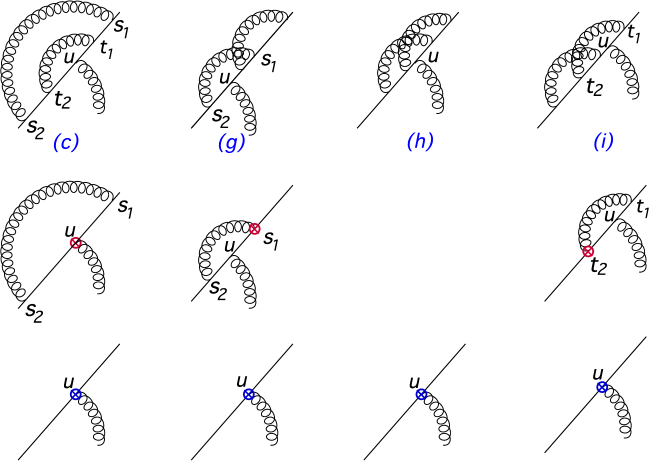
Figure 11: Renormalization of the (5,1) web. Upper row: the boomerang gluon subdiagram in diagrams $(c)$, $(g)$, $(h)$ and $(i)$; Second row: one-loop counterterm contributions to the above diagrams associated with shrinking the innermost boomerang gluon to a point; Third row: two-loop counterterm contributions to the above diagrams associated with simultaneously shrinking both boomerang gluons to a point.

In diagram $(c)$, a one-loop counterterm is required to compensate for the subdivergence associated with shrinking the innermost boomerang gluon to the emission vertex of the non-boomerang gluon at point $u$, going to the second line in fig. 11. The remaining diagram after this contraction is the mushroom graph of figure 2$(a)$, which was computed in section 3.2. An additional renormalization is required to compensate for the divergence associated with shrinking both gluons to a point, going to the third row in fig. 11. The remaining diagram is simply the one gluon exchange diagram. Similarly, one- and two-loop counterterms are required for diagrams $(g)$ and $(i)$, with the only difference to the above being that now the first boomerang gluon being shrunk renormalizes one of the vertices of the second, rather than the non-boomerang emission vertex. Finally, diagram $(h)$ has no one-loop subdivergences, as each of the boomerang gluons straddles two emission vertices, but it does require a two-loop counterterm corresponding to shrinking both boomerang gluons simultaneously to a point.

As implied by the above description, the required counterterm contributions can be all identified considering the boomerang subdiagrams in fig. 11, without reference to the integration over $u$ nor the other Wilson line. We therefore proceed to compute these considering the pole terms in the integrand of eq. (5.36). To this end we introduce an upper limit on the furthest boomerang gluon attachment along the Wilson line, which we denote by $u_{\max}$, and consider the poles arising in $\mathcal{B}_{i}^{[0,u_{\max}]}(u)$ for each of the contributing diagrams. For diagram $(c)$ we find

$$\begin{split}\mathcal{B}_{c}^{[0,u_{\max}]}(u)=\,&\bar{\mu}^{4\epsilon}(-\beta_{1}^{2})^{2\epsilon}g_{s}^{4}\mathcal{N}^{2}\int^{u}_{0}ds_{2}\int_{s_{2}}^{u}dt_{2}\int^{u_{\max}}_{u}ds_{1}\int_{u}^{s_{1}}dt_{1}\,((s_{1}-s_{2})^{2})^{\epsilon-1}((t_{1}-t_{2})^{2})^{\epsilon-1}\\ =\,&\Big{(}\frac{g_{s}^{2}}{4\pi^{2}}\Big{)}^{2}\bigg{\{}\frac{1}{8\,\epsilon^{2}}+\frac{1}{4\,\epsilon}\Big{[}1+2\gamma_{E}+2\,\text{ln}\Big{(}\frac{\sqrt{-\beta_{1}^{2}}\mu(u_{\max}-u)u}{u_{\max}}\Big{)}\Big{]}+\mathcal{O}(\epsilon^{0})\bigg{\}},\end{split}$$ (5.40)

where in the second line we performed the four integrations and expanded in $\epsilon$, discarding finite terms. Similarly, for the remaining diagrams we find

$$\mathcal{B}_{g}^{[0,u_{\max}]}(u)=\, \Big{(}\frac{g_{s}^{2}}{4\pi^{2}}\Big{)}^{2}\bigg{\{}\frac{1}{8\,\epsilon^{2}}+\frac{1}{2\,\epsilon}\Big{[}1+\gamma_{E}+\text{ln}\Big{(}\frac{\sqrt{-\beta_{1}^{2}}\mu(u_{\max}-u)u}{u_{\max}}\Big{)}\Big{]}+\mathcal{O}(\epsilon^{0})\bigg{\}};$$

$$\mathcal{B}_{h}^{[0,u_{\max}]}=\, \Big{(}\frac{g_{s}^{2}}{4\pi^{2}}\Big{)}^{2}\bigg{\{}\frac{1}{4\,\epsilon}+\mathcal{O}(\epsilon^{0})\bigg{\}};$$

$$\mathcal{B}_{i}^{[0,u_{\max}]}(u)=\, \Big{(}\frac{g_{s}^{2}}{4\pi^{2}}\Big{)}^{2}\bigg{\{}\frac{1}{8\,\epsilon^{2}}+\frac{1}{2\,\epsilon}\Big{[}1+\gamma_{E}+\text{ln}\Big{(}\frac{\sqrt{-\beta_{1}^{2}}\mu(u_{\max}-u)u}{u_{\max}}\Big{)}\Big{]}+\mathcal{O}(\epsilon^{0})\bigg{\}}.$$ (5.41)

Note that diagram $(h)$, being free of one-loop subdivergences, does not have a double pole, nor does its single-pole carry any dependence on the position of the non-boomerang attachment $u$ and the cutoff $u_{\max}$.

Next, consider the counterterm contributions removing the one-loop subdivergences in diagrams $(c)$, $(g)$ and $(i)$ described by the second row in fig. 11. These three diagrams are all the same: they simply correspond to the one-loop counterterm $Z_{v}^{(1)}$ of eq. (C.4) times

$$\begin{split}{\cal B}_{M}^{[0,u_{\max}]}(u)=\,&-\bar{\mu}^{2\epsilon}(-\beta_{1}^{2})^{\epsilon}g_{s}^{2}\mathcal{N}\int^{u_{\max}}_{u}ds_{1}\int^{u}_{0}ds_{2}((s_{1}-s_{2})^{2})^{\epsilon-1}\\ =\,&\,\bar{\mu}^{2\epsilon}(-\beta_{1}^{2})^{\epsilon}g_{s}^{2}\mathcal{N}\frac{u_{\max}^{2\epsilon}-(u_{\max}-u)^{2\epsilon}-u^{2\epsilon}}{2\epsilon(1-2\epsilon)},\end{split}$$ (5.42)

where the subscript $M$ indicates that this function forms the integrand of the mushroom diagram, that is inserting ${\cal B}_{M}^{[0,u_{\max}]}(u)$ into eq. (5.36) and sending $u_{\max}\to\infty$, one recovers the mushroom diagram of section 3.2. Upon expanding eq. (5.42) in $\epsilon$ and multiplying by $Z_{v}^{(1)}$ of eq. (C.4) we obtain:

$$Z_{v}^{(1)}{\cal B}_{M}^{[0,u_{\max}]}(u)=\Big{(}\frac{g_{s}^{2}}{4\pi^{2}}\Big{)}^{2}\bigg{\{}-\frac{1}{4\epsilon^{2}}-\frac{1}{2\epsilon}\Big{[}1+\gamma_{E}+\text{ln}\Big{(}\frac{\sqrt{-\beta_{1}^{2}}\mu(u_{\max}-u)u}{u_{\max}}\Big{)}\Big{]}+\mathcal{O}(\epsilon^{0})\bigg{\}}.$$ (5.43)

To complete the renormalization of the web we proceed to determine the relevant two-loop counterterm by requiring that the sum of all contributions to the web, weighted by the appropriate exponentiated colour factors displayed in the second line of eq. (5.35), is ultraviolet finite:

$$\begin{split}&\Big{(}\mathcal{B}_{c}^{[0,u_{\max}]}(u)+Z_{v}^{(1)}{\cal B}_{M}^{[0,u_{\max}]}(u)+Z_{v(c)}^{(2)}\Big{)}+\Big{(}\mathcal{B}_{g}^{[0,u_{\max}]}(u)+Z_{v}^{(1)}{\cal B}_{M}^{[0,u_{\max}]}(u)+Z_{v(g)}^{(2)}\Big{)}\\ &+2\Big{(}\mathcal{B}_{h}^{[0,u_{\max}]}(u)+Z_{v(h)}^{(2)}\Big{)}+\Big{(}\mathcal{B}_{i}^{[0,u_{\max}]}(u)+Z_{v}^{(1)}{\cal B}_{M}^{[0,u_{\max}]}(u)+Z_{v(i)}^{(2)}\Big{)}=\mathcal{O}(\epsilon^{0}),\end{split}$$ (5.44)

It is straightforward to verify that for each of the three diagrams $(c)$, $(g)$ and $(i)$ the logarithmic dependence on the position of the non-boomerang attachment $u$ and the cutoff $u_{\max}$ cancels with the corresponding $Z_{v}^{(1)}{\cal B}_{M}^{[0,u_{\max}]}(u)$ counterterm. Ultraviolet finiteness of the sum of diagrams in eq. (5.44) fixes the two-loop vertex renormalization factor associated with multiple gluon exchange graphs to be

$$\begin{split}Z_{v({\rm MGE})}^{(2)}\equiv Z_{v(c)}^{(2)}+Z_{v(g)}^{(2)}+2Z_{v(h)}^{(2)}+Z_{v(i)}^{(2)}=&\Big{(}\frac{g_{s}^{2}}{4\pi^{2}}\Big{)}^{2}\bigg{\{}\frac{3}{8\,\epsilon^{2}}-\frac{1}{4\,\epsilon}\bigg{\}}.\end{split}$$ (5.45)

The total contribution to the web from the second-order counterterm may be written as $Z_{v({\rm MGE})}^{(2)}$ multiplying the one-gluon exchange web:

$$\begin{split}Z_{v({\rm MGE})}^{(2)}\mathcal{F}^{(1)}_{(1,1)}&=\left(\frac{g_{s}^{2}}{8\pi^{2}}\right)^{3}\int_{0}^{1}dzp_{\epsilon}(z,\alpha_{12})\left\{\frac{1}{\epsilon^{2}}\left[2+\frac{3}{2}\ln z+\frac{3}{4}\ln\left(\frac{\mu^{2}}{m^{2}}\right)\right]+\frac{1}{\epsilon}\left[3+\frac{3\pi^{2}}{4}\right.\right.\\ &\left.\left.+3\ln z+\frac{3}{2}\ln^{2}z+\ln\left(\frac{\mu^{2}}{m^{2}}\right)\left(\frac{7}{2}+3\ln z\right)+\frac{9}{8}\ln^{2}\left(\frac{\mu^{2}}{m^{2}}\right)\right]\right\}.\end{split}$$ (5.46)

The total renormalized web is now given by

$$W_{(5,1)}=c_{1}^{[3,2]}\Big{[}{\cal F}_{c}+{\cal F}_{g}+2{\cal F}_{h}+{\cal F}_{i}+3Z_{v}^{(1)}{\cal F}_{M}+Z_{v({\rm MGE})}^{(2)}\mathcal{F}^{(1)}_{(1,1)}\Big{]},$$ (5.47)

where ${\cal F}_{M}$ denotes the mushroom graph of figure 2$(a)$. As in other two-line webs no additional subtraction of commutators is necessary and thus, the contribution of the (5,1) web to the soft anomalous dimension is directly given by the single-pole contribution to eq. (5.47). Combining all contributions leads to

$$F^{(3)}_{(5,1);1}(\alpha_{12})=\int_{0}^{1}dx_{1}p_{0}(x_{1},\alpha_{12}){\cal G}^{(3)}_{(5,1);1}(x_{1},\alpha_{12}),$$ (5.48)

where the appropriate web kernel is

$${\cal G}^{(3)}_{(5,1);1}(x_{1},\alpha_{12}) =-8\left[\frac{4}{3}-\frac{\pi^{2}}{9}-\frac{5}{6}\ln\left(\frac{q(x_{1},\alpha_{12})}{x_{1}^{2}}\right)+\frac{1}{8}\ln^{2}\left(\frac{q(x_{1},\alpha_{12})}{x_{1}^{2}}\right)\right].$$ (5.49)

Finally, performing the integration over $x_{1}$ we readily obtain the result in terms of the basis functions $M_{k,l,n}(\alpha_{ij})$ of eq. (2.50):

$$F^{(3)}_{(5,1);1}(\alpha_{12})=-8r(\alpha_{12}) \left[\frac{4}{3}M_{0,0,0}(\alpha_{12})-\frac{1}{3}M_{0,2,0}(\alpha_{12})+\frac{1}{12}M_{0,0,2}(\alpha_{12})-\frac{5}{6}M_{1,0,0}(\alpha_{12})\right.$$

$$\left.\quad+\frac{1}{8}M_{2,0,0}(\alpha_{12})\right].$$ (5.50)

We confirm once more the pattern described following eq. (5.11). Indeed, the (5,1) web can also be expressed in terms of these basis functions, and similarly to other boomerang webs it features mixed, non-maximal weights, here weights 3, 2 and 1.

5.2.3 The (2,4) web

The last remaining boomerang web is the (2,4) web of figure 4 where, as already discussed, only diagrams $(a)$ through $(f)$ will contribute to the final result. Applying a replica analysis to obtain the web mixing matrix, we find (after applying colour algebra) that the corresponding exponentiated colour factors are given by

$$\tilde{C}(a) =-\frac{1}{2}c_{1}^{[3,2]}+c_{2}^{[3,2]};$$

$$\tilde{C}(b) =-\frac{3}{2}c_{1}^{[3,2]}+c_{2}^{[3,2]};$$

$$\tilde{C}(c) =\tilde{C}(d)=0$$

$$\tilde{C}(e) =\tilde{C}(f)=-c_{1}^{[3,2]},$$ (5.51)

so that the contribution of the entire renormalised web is given by

$$W_{(2,4)}= \,c^{[3,2]}_{1}\Big{[}{\cal F}_{(2,4);1}+{\cal F}_{(2,4);1}^{\rm CT}\Big{]}+c^{[3,2]}_{2}\Big{[}{\cal F}_{(2,4);2}\Big{]}$$ (5.52)

$$= -c^{[3,2]}_{1}\left(\frac{1}{2}{\cal F}_{a}+\frac{3}{2}{\cal F}_{b}+{\cal F}_{e}+{\cal F}_{f}+{\cal F}_{e}^{\rm CT}+{\cal F}_{f}^{\rm CT}\right)+c^{[3,2]}_{2}\left({\cal F}_{a}+{\cal F}_{b}\right)\,,$$

As indicated in the second line, ${\cal F}_{(2,4);1}^{\rm CT}$ is included because diagrams $(e)$ and $(f)$ must be supplemented by graphs in which the one-loop vertex counterterm of appendix C dresses the two-loop crossed gluon web of figure 19, whose kinematic factor can be found in eqs. (A.3, A.4). This gives

$${\cal F}_{(2,4);1}^{\rm CT}=-2Z_{v}^{(1)}{\cal F}_{X}.$$ (5.53)

Using the calculational approach adopted for the other boomerang webs, we find that the kinematic part of each diagram $D\in\{a,b,e,f\}$ in figure 4 can be written as

$${\cal F}_{D}(\alpha_{12})=\kappa^{3}\frac{\Gamma(6\epsilon)}{\epsilon(1-2\epsilon)}\int_{0}^{1}dy\,dz\,p_{\epsilon}(y,\alpha_{12})p_{\epsilon}(z,\alpha_{12})\phi_{D}(y,z;\alpha_{12})\,,$$ (5.54)

where we have already performed the integration over the boomerang gluon. Considering first diagram $(a)$ we find

$$\begin{split}\phi_{a}(y,z;\alpha_{12})=(1-y)^{2\epsilon}\int_{0}^{1}dw\,w^{4\epsilon-1}(1-w)^{2\epsilon-1}&\bigg{[}1-\bigg{(}1-\frac{1-w}{w}\frac{1-z}{1-y}\bigg{)}^{2\epsilon}\bigg{]}\\ &\times\theta\bigg{(}\frac{1-w}{w}<\frac{y}{z}\bigg{)}\theta\bigg{(}\frac{1-w}{w}<\frac{1-y}{1-z}\bigg{)}.\end{split}$$ (5.55)

Making the change of variable to:

$$q=\frac{1-w}{w},$$ (5.56)

eq. (5.55) becomes:

$$\phi_{a}(y,z;\alpha_{12})=(1-y)^{2\epsilon}\int_{0}^{\infty}dq\hskip 2.84544ptq^{2\epsilon-1}(1+q)^{-6\epsilon}\bigg{[}1-\bigg{(}1-\frac{1-z}{1-y}q\bigg{)}^{2\epsilon}\bigg{]}\theta\bigg{(}q<\frac{y}{z}\bigg{)}\theta\bigg{(}q<\frac{1-y}{1-z}\bigg{)}\,,$$ (5.57)

which can be integrated to give

$$\begin{split}\phi_{a}&(y,z;\alpha_{12})=\frac{(1-y)^{2\epsilon}}{2\epsilon}\times\\ &\Bigg{\{}\Big{(}\frac{y}{z}\Big{)}^{2\epsilon}\theta(z>y)\Bigg{[}{}_{2}F_{1}\left(2\epsilon,6\epsilon;1+2\epsilon;-\frac{y}{z}\right)-F_{1}\left(2\epsilon,6\epsilon,-2\epsilon,1+2\epsilon;-\frac{y}{z},\frac{y(1-z)}{z(1-y)}\right)\Bigg{]}\,+\\ &\Big{(}\frac{1-y}{1-z}\Big{)}^{2\epsilon}\theta(y>z)\Bigg{[}{}_{2}F_{1}\left(2\epsilon,6\epsilon;1+2\epsilon;-\frac{1-y}{1-z}\right)-\frac{\Gamma^{2}(1+2\epsilon)}{\Gamma(1+4\epsilon)}{{}_{2}}F_{1}\left(2\epsilon,6\epsilon;1+4\epsilon;-\frac{1-y}{1-z}\right)\Bigg{]}\Bigg{\}}.\end{split}$$ (5.58)

Here ${{}_{2}}F_{1}(a,b;c;z)$ is the Gauss hypergeometric function, and $F_{1}(a,b,c,d;x,y)$ the Appell $F_{1}$ function. We may expand the former in $\epsilon$ using the HypExp package in Mathematica [75, 76]. We explain how to expand the Appell function in appendix F.1, such that after expansion in $\epsilon$ eq. (5.58) assumes the form

$$\phi_{a}(y,z;\alpha_{12})=2\epsilon\,\,\text{Li}_{2}\Big{(}\frac{z}{y}\frac{1-y}{1-z}\Big{)}\,\theta(y>z)+2\epsilon\,\zeta_{2}\theta(z>y)+{\cal O}(\epsilon^{2})\,.$$ (5.59)

Next we note that owing to the symmetry of the propagator functions in (5.54), we are free to transform the integration parameters according to $y\rightarrow 1-y$ and $z\rightarrow 1-z$, in any of the terms. Using this freedom we eliminate the $\theta(z>y)$ component, shifting the $\zeta_{2}$ term to the $\theta(y>z)$ component, obtaining

$$\phi_{a}(y,z;\alpha_{12})=\epsilon\,\bigg{\{}2\,\zeta_{2}+2\,\text{Li}_{2}\Big{(}\frac{z}{y}\frac{1-y}{1-z}\Big{)}\bigg{\}}\,\theta(y>z)+{\cal O}(\epsilon^{2}).$$ (5.60)

Similarly, the kinematic parts of diagrams $(b)$, $(e)$ and $(f)$ in figure 4 can be written in the form of eq. (5.54) with the kernels

$$\phi_{D}(y,z;\alpha_{12}) =(1-y)^{2\epsilon}\int_{0}^{\infty}dq\,q^{2\epsilon-1}(1+q)^{-6\epsilon}\theta\bigg{(}q>\frac{y}{z}\bigg{)}\theta\left(q<\frac{1-y}{1-z}\right)\,\,\psi_{D}\left(\displaystyle{\frac{1-z}{1-y}q}\right)$$ (5.61)

where

$$\begin{split}\psi_{b}(Q)&=1-\psi_{f}(Q);\qquad\psi_{e}(Q)=Q^{2\epsilon}-\psi_{b}(Q);\qquad\psi_{f}(Q)=\left(1-Q\right)^{2\epsilon}\,.\end{split}$$ (5.62)

The corresponding $\epsilon$-expanded kernels are given by

$$\phi_{b}(y,z;\alpha_{12})= \,\epsilon\,\bigg{\{}2\,\zeta_{2}-2\,\text{Li}_{2}\Big{(}\frac{z}{y}\frac{1-y}{1-z}\Big{)}\bigg{\}}\,\theta(y>z)+{\cal O}(\epsilon^{2});$$ (5.63)

$$\phi_{e}(y,z;\alpha_{12})= \,\bigg{\{}\text{ln}\Big{(}\frac{y}{z}\frac{1-z}{1-y}\Big{)}+\Big{[}\frac{1}{2}\text{ln}^{2}\Big{(}\frac{1-z}{1-y}\Big{)}-\frac{1}{2}\text{ln}^{2}\Big{(}\frac{z^{2}}{y^{2}}\frac{1-y}{1-z}\Big{)}+2\,\text{ln}\Big{(}\frac{y}{z}\frac{1-z}{1-y}\Big{)}\text{ln}(1-z)$$

$$-2\,\zeta_{2}+6\,\text{Li}_{2}\Big{(}-\frac{1-z}{1-y}\Big{)}-6\,\text{Li}_{2}\Big{(}-\frac{z}{y}\Big{)}+2\,\text{Li}_{2}\Big{(}\frac{z}{y}\frac{1-y}{1-z}\Big{)}\Big{]}\epsilon\,\bigg{\}}\,\theta(y>z)+{\cal O}(\epsilon^{2});$$

$$\phi_{f}(y,z;\alpha_{12})= \,\bigg{\{}\text{ln}\Big{(}\frac{y}{z}\frac{1-z}{1-y}\Big{)}+\Big{[}\text{ln}^{2}\Big{(}\frac{1-z}{1-y}\Big{)}-\text{ln}^{2}\Big{(}\frac{z}{y}\Big{)}+2\,\text{ln}\Big{(}\frac{y}{z}\frac{1-z}{1-y}\Big{)}\text{ln}(1-z)-2\,\zeta_{2}$$

$$+6\,\text{Li}_{2}\Big{(}-\frac{1-z}{1-y}\Big{)}-6\,\text{Li}_{2}\Big{(}-\frac{z}{y}\Big{)}+2\,\text{Li}_{2}\Big{(}\frac{z}{y}\frac{1-y}{1-z}\Big{)}\Big{]}\epsilon\,\bigg{\}}\,\theta(y>z)+{\cal O}(\epsilon^{2}).$$

The combination of kinematic factors appearing in eq. (5.52) for the colour factor $c_{1}^{[3,2]}$ then evaluates to

$$\begin{split}&{\cal F}_{(2,4);1}(\alpha_{12})=-\left(\frac{g_{s}^{2}}{8\pi^{2}}\right)^{3}\int_{0}^{1}dy\,dz\,p_{0}(y,\alpha_{12})p_{0}(z,\alpha_{12})\theta(y>z)\\ &\times\left\{\frac{1}{6}\left[-12{\rm Li}_{2}\left(-\frac{1-z}{1-y}\right)+12{\rm Li}_{2}\left(-\frac{z}{y}\right)-2{\rm Li}_{2}\left(\frac{z(1-y)}{y(1-z)}\right)+2\ln\left(\frac{z(1-y)}{y(1-z)}\right)\ln\left(\frac{q(y,\alpha_{12})}{y^{2}}\right)\right.\right.\\ &\left.\left.\quad-2\ln\left(\frac{y}{1-y}\right)\ln\left(\frac{q(z,\alpha_{12})}{z^{2}}\right)-2\ln\left(\frac{1-z}{z}\right)\log\left(\frac{q(z,\alpha_{12})}{(1-z)^{2}}\right)-6\ln\left(\frac{y}{1-y}\right)\ln\left(\frac{1-z}{z}\right)\right.\right.\\ &\left.\left.\quad-4\ln\left(\frac{y(1-z)}{z(1-y)}\right)-12\ln z\ln\left(\frac{y(1-z)}{z(1-y)}\right)-\ln^{2}\left(\frac{y}{1-y}\right)-9\ln^{2}\left(\frac{1-z}{z}\right)\right]\right.\\ &\left.\quad-\ln\left(\frac{\mu^{2}}{m^{2}}\right)\ln\left(\frac{y(1-z)}{z(1-y)}\right)\right\}\frac{1}{\epsilon}+{\cal O}(\epsilon^{0}).\end{split}$$ (5.64)

Furthermore, the counterterm contribution amounts to

$$\begin{split}{\cal F}_{(2,4);1}^{\rm CT}(\alpha_{12})&=-\frac{1}{2}\left(\frac{g_{s}^{2}}{8\pi^{2}}\right)^{3}\int_{0}^{1}dy\,dz\,p_{0}(y,\alpha_{12})p_{0}(z,\alpha_{12})\theta(y>z)\left\{\ln\left(\frac{y(1-z)}{z(1-y)}\right)\left[2\ln\left(\frac{\mu^{2}}{m^{2}}\right)\right.\right.\\ &\left.\left.+\ln\left(\frac{q(y,\alpha_{12})}{y^{2}}\right)+\ln\left(\frac{q(z,\alpha_{12})}{z^{2}}\right)+2\ln(yz)\right]+4{\rm Li}_{2}\left(-\frac{1-z}{1-y}\right)-4{\rm Li}_{2}\left(-\frac{z}{y}\right)\right.\\ &\left.+\ln^{2}\left(\frac{1-z}{1-y}\right)-\ln^{2}\left(\frac{z}{y}\right)\right\}\frac{1}{\epsilon}+{\cal O}(\epsilon^{0}).\end{split}$$ (5.65)

Using the fact that there are no lower-order contributions that form non-zero commutators in eq. (2.1), the ${\cal O}(\epsilon^{-1})$ coefficient of the renormalized (2,4) web directly determine its contribution to the soft anomalous dimension. Putting things together in the combination of eq. (5.52), we find the integrals multiplying the two colour structures $c_{i}^{[3,2]}$ for $i=1,2$ to be

$$F_{(2,4);i}^{(3)}(\alpha_{12})=\int_{0}^{1}dy\int_{0}^{1}dz\,p_{0}(y,\alpha_{12})\,p_{0}(z,\alpha_{12})\,\theta(y>z)\,{\cal G}_{(2,4);i}^{(3)}(y,z,\alpha_{12})\,,$$ (5.66)

where we displayed the overall Heaviside function restricting the integration range, and where

$${\cal G}^{(3)}_{(2,4);1}(y,z,\alpha_{12}) =\frac{4}{3}\bigg{[}2\,\text{Li}_{2}\Big{(}\frac{z}{y}\frac{1-y}{1-z}\Big{)}+4\,\text{ln}\Big{(}\frac{y}{1-y}\Big{)}-\text{ln}\Big{(}\frac{y}{1-y}\Big{)}\text{ln}\Big{(}\frac{q(y,\alpha_{12})}{y^{2}}\Big{)}-2\,\text{ln}^{2}\Big{(}\frac{y}{1-y}\Big{)}$$

$$+4\,\text{ln}\Big{(}\frac{1-z}{z}\Big{)}-\text{ln}\Big{(}\frac{1-z}{z}\Big{)}\text{ln}\Big{(}\frac{q(z,\alpha_{12})}{(1-z)^{2}}\Big{)}-\text{ln}\Big{(}\frac{y}{1-y}\Big{)}\text{ln}\Big{(}\frac{q(z,\alpha_{12})}{z^{2}}\Big{)}$$

$$+\text{ln}\Big{(}\frac{z}{1-z}\Big{)}\text{ln}\Big{(}\frac{q(y,\alpha_{12})}{y^{2}}\Big{)}\bigg{]};$$

$${\cal G}^{(3)}_{(2,4);2}(y,z,\alpha_{12}) =-\frac{16}{3}\zeta_{2}\,.$$ (5.67)

The second kernel can be straightforwardly integrated over $y$ and $z$ and written in terms of the basis functions of eq. (2.50) as

$$F^{(3)}_{(2,4);2}(\alpha_{12})=-\frac{4}{9}r^{2}(\alpha_{12})\pi^{2}M_{0,0,0}^{2}(\alpha_{12})=-\frac{4}{9}r^{2}(\alpha_{12})\Big{(}6M_{0,2,1}(\alpha_{12})-M_{0,0,3}(\alpha_{12})\Big{)}\,.$$ (5.68)

The integration of the first kernel in eq. (5.67), however, is not immediately interpretable in terms of basis functions. Firstly, it contains dilogarithms involving the parameters $y$ and $z$, which are not part of the integrand of eq. (2.50), consisting exclusively of powers of logarithms. The webs previously calculated in this paper and in refs. [44, 45] contained dilogarithms at intermediate stages, but these completely cancelled at the level of the subtracted web integrand. Here this is not the case, and we have furthermore found no variable transformation (or dilogarithm identity) that removes the dilogarithms from eq. (5.67). Secondly, there is a remaining Heaviside function in eq. (5.67), which also does not appear in the definition of eq. (2.50). It thus appears that our previously conjectured basis of functions is incomplete. However, this conclusion is premature and incorrect. Remarkably, the kernel of eq. (5.67) may be integrated fully analytically and found to respect the basis of eq. (2.50) after all. In appendix F.2 we show how this works in detail. The final result reads

$$\begin{split}F^{(3)}_{(2,4);1}(\alpha_{12})&=\frac{4}{3}r^{2}(\alpha_{12})\Big{[}8M_{0,1,1}(\alpha_{12})-4M_{1,1,1}(\alpha_{12})-3M_{0,2,1}(\alpha_{12})-\frac{1}{6}\,M_{0,0,3}(\alpha_{12})\Big{]}\,,\end{split}$$ (5.69)

featuring weight 4 as well as weight 3 contributions.

We have now calculated all multiple-gluon exchange boomerang webs up to three-loop order, and shown that they conform with the expected functional form: an overall rational function consisting of powers of $r({\alpha_{ij}})$ for any non-boomerang exchange between lines $i$ and $j$, multiplying a pure transcendental function. The latter may be expressed in terms of sums of products of our $M_{k,l,n}(\alpha_{ij})$ basis functions, each dependent on a single $\alpha_{ij}$ and having a restricted symbol alphabet, eq. (2.47). We found one salient difference compared to non-boomerang MGEWs: while MGEWs without boomerang gluons have uniform, maximal weight (weight 5 for subtracted webs at three loops), boomerang ones have mixed, non-maximal weight. Table 2 presents the weights occurring in each case:

web	boomerangs	weights
(1,1,4)  $c^{[3,3]}_{3}$	1	4
(1,1,4)  $c^{[3,3]}_{4}$	1	4,3
(1,2,3)  $c^{[3,3]}_{4}$	1	4,3,2
(3,3)  $c^{[3,2]}_{1}$	2	3,2
(5,1)  $c^{[3,2]}_{1}$	2	3,2,1
(2,4)  $c^{[3,2]}_{2}$	1	4
(2,4)  $c^{[3,2]}_{1}$	1	4,3

Table 2: Transcendental weights in the kinematic functions of three-loop webs. The left column specifies the web and the colour factor component using the bases in eqs. (5.1) and (5.25), the middle column presents the number of boomerang gluons, and the right one the weights of the transcendental functions entering the anomalous dimension.

the fact that the maximal weight occurring reduces by one unit with each additional boomerang gluon, is expected based on the observation in section 3.3, namely that for each boomerang gluon, there is one integration, over $x_{l}$ in eq. (3.23), which instead of increasing the weight by one unit as in non-boomerang webs, generates a factor of $1/(1-2\epsilon)$, which reflects a power divergence due to an instantaneous interaction. At leading order in the $\epsilon$ expansion this readily translates into a weight drop compared to the non-boomerang case, and furthermore, when subleading powers in $\epsilon$ hit higher-order pole terms in the web kernel, further lower weight terms emerge.

As discussed in section 2.3, a further consistency check on higher-loop webs is that a subset of the information in a given web can be obtained from webs connecting a greater number of Wilson lines, through the process of collinear reduction. We discuss how this applies to the boomerang webs calculated in this paper in the following section.

6 Collinear reduction for boomerang webs

In section 2, we reviewed how kinematic factors have been previously obtained for boomerang-free MGEWs [55, 57, 58, 44, 45]. In such cases, it was possible to perform an additional (albeit partial) cross-check of the final results for web kinematic factors, using the process of collinear reduction [45]. Roughly speaking, this states that one may take a web connecting $n$ Wilson lines, and obtain kinematic results pertaining to webs connecting $m<n$ lines, by identifying the 4-velocities of two or more Wilson lines in the original web. In carrying out such a procedure, gluon emissions from different Wilson lines may end up on the same line, and we must then reinterpret the colour indices of such emissions appropriately. To this end, the effective vertex formalism reviewed here in section 2.3 becomes useful: eq. (2.25) implies that there is no natural ordering of effective vertices if more than one of them occurs on a given Wilson line. Thus, as far as the ordering of vertices is concerned, it is similar to the case where they occur on different Wilson lines. To explore the converse of this, imagine a web in which two Wilson lines $l_{1}$ and $l_{2}$ contain a single vertex each, which we may write as $V_{K_{1}}^{(l_{1})}$ and $V_{K_{2}}^{(l_{2})}$ respectively. The collinear reduction process then consists of the following steps:

1. One sets the 4-velocities $\beta_{1}$ and $\beta_{2}$ to be equal (hence the term “collinear”).

2. One identifies the partonic colour indices of the generators in the two vertices as living in the same (single) colour space.

3. One symmetrises over the colour factors of the two vertices, as in eq. (2.25).

4. One must include symmetry factors present in the obtained web, that are missing in the original web.

This procedure generalises straightforwardly to any number of effective vertices, and was already used in ref. [45], where it provided a highly non-trivial check of non-boomerang MGEWs at three-loop order. Note that not all information in the fewer-line webs can be obtained by collinear reduction. Due to the symmetrisation over multiple vertices, the fully antisymmetric colour part of a given web cannot be generated. This is precisely the contribution in which there is a fully connected colour factor on each individual Wilson line, namely that arising from having at most a single effective vertex on each line. For example, for three-line webs collinear reduction may yield the components involving $c_{i}^{[3,3]}$ for $i=1$ through $3$ in eq. (5.1), which contain two $C_{2,1}$ effective vertices (defined in eq. (2.23)) on line $i$, but not $c_{4}^{[3,3]}$, which is fully antisymmetric. Similarly for two-line webs collinear reduction may yield the $c_{2}^{[3,2]}$ component defined in eq. (5.25), but not the $c_{1}^{[3,2]}$ one.

It is possible to use a similar collinear reduction procedure to check some of the results of this paper. However, the presence of boomerang gluons creates additional complications, which were not necessary to consider in ref. [45]. At the outset, in computing non-boomerang MGEWs using collinear reduction, the collinear limit $\beta_{i}=\beta_{j}$ simply amounts to identifying $\alpha_{ik}=\alpha_{jk}$ in the kinematic function of the original web. In turn, in computing boomerang webs, the collinear limit also involves taking $\alpha_{ij}\to-1$ for the boomerang gluon itself. In this limit $r(\alpha_{ij})$ of eq. (2.45) diverges and the basis functions $M_{k,l,n}(\alpha_{ij})$ become complex, so it is not a priori clear that the collinear limit exists. To better understand the problem we first consider the relation between the single-gluon exchange (1,1) web diagram and the self-energy one upon taking the collinear limit. We will subsequently explain how the problem is resolved in boomerang webs in which boomerang gluons straddle one or more emissions along the Wilson line. We will demonstrate the application of the collinear reduction procedure in the rather non-trivial example of the (1,1,4) web in section 6.2.

6.1 The collinear limit of the (1,1) web

In this section, we consider the (1,1) web of figure 12($a$) and use it to analyse the collinear limit. Upon identifying the two Wilson lines $i$ and $j$, we obtain the self-energy diagram of figure 12($b$), whose integral was computed in section 3.1.

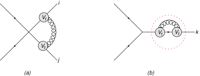
Figure 12: ($a$) The (1,1) web, which features a 1-gluon emission vertex on each line; ($b$) collinear reduction of Wilson lines $i$ and $j$ to make a self-energy web on the single line $i$.

The kinematic factor for the (1,1) web is given in eq. (A.1),

$$\mathcal{F}^{(1)}(\alpha_{ij},\epsilon)\,=\,\kappa\Gamma(2\epsilon)\int_{0}^{1}dxp_{\epsilon}(x,\alpha_{ij})=\frac{\kappa}{\epsilon}\,\frac{1+\alpha_{ij}^{2}}{1-\alpha_{ij}^{2}}\ln(\alpha_{ij})+\,{\cal O}(\epsilon^{0})\,,$$ (6.1)

where in the second equality we substituted for $r(\alpha_{ij})$ using eq. (2.45) and expanded in $\epsilon$, keeping only the leading-order term. Taking the collinear limit to obtain figure 12($b$), one identifies $\beta_{i}=\beta_{j}$, which from eq. (2.5) implies

$$\gamma_{ij}\rightarrow 2,\quad\alpha_{ij}\rightarrow-1.$$ (6.2)

One could therefore expect that the self-energy web would be given by the $\alpha_{ij}\rightarrow-1$ limit of eq. (6.1), that is

$$\frac{1}{2}\lim_{\alpha_{ij}\rightarrow-1}\mathcal{F}^{(1)}(\alpha_{ij},\epsilon)\,=\,\frac{1}{2}\frac{\kappa}{\epsilon}\lim_{\alpha_{ij}\rightarrow-1}\,\frac{1+\alpha_{ij}^{2}}{1-\alpha_{ij}^{2}}\ln(\alpha_{ij})+\cdots\,=\,\frac{1}{2}\frac{\kappa}{\epsilon}\lim_{\alpha_{ij}\rightarrow-1}\,\frac{i\pi}{1+\alpha_{ij}}+\cdots,$$ (6.3)

where the factor of $1/2$ originates from the symmetrisation of the colour generators. Perhaps surprisingly, we see that the kinematic limit required for the collinear reduction is ill-defined, whereas the result we are expecting to reproduce – the self-energy factor of eq. (3.5) – is perfectly well-behaved.

To see what has gone wrong, we may examine the kinematic factor for the (1,1) web in more detail. Following the procedures outlined in section 2, one finds (cf. eq. (3.2))

$${\cal F}_{(1,1)}^{(1)}(\alpha_{ij}) =g_{s}^{2}\bar{\mu}^{2\epsilon}{\cal N}\beta_{i}\cdot\beta_{j}\int_{0}^{\infty}ds\int_{0}^{\infty}dt\left[-(s\beta_{i}-t\beta_{j})^{2}+i\varepsilon\right]^{\epsilon-1}\,e^{-im\left(s\sqrt{\beta_{i}^{2}}+t\sqrt{\beta_{j}^{2}-i\varepsilon}\right)},\,$$ (6.4)

where $s$ and $t$ are distance variables for the gluon attachments on lines $i$ and $j$ respectively. Transforming according to eqs. (2.31, 2.32), eq. (6.4) can be rewritten as

$${\cal F}_{(1,1)}^{(1)}(\alpha_{ij}) =\kappa\gamma_{ij}\int_{0}^{\infty}d\lambda\lambda^{2\epsilon-1}e^{-\lambda}\int_{0}^{1}dx\left[x^{2}+(1-x)^{2}-\gamma_{ij}x(1-x)\right]^{\epsilon-1}\,$$

$$=-\kappa\Gamma(2\epsilon)\left(\alpha_{ij}+\frac{1}{\alpha_{ij}}\right)\int_{0}^{1}dx\left[x^{2}+(1-x)^{2}+\left(\alpha_{ij}+\frac{1}{\alpha_{ij}}\right)x(1-x)\right]^{\epsilon-1},$$ (6.5)

where the $\lambda$ integral was carried out as previously. In general kinematics one may subsequently perform the integration over $x$ using the factorization property of the expression in the square brackets ($q(x,\alpha)$ in eq. (2.42)) yielding the hypergeometric functions in eq. (A.1) corresponding to the two poles at

$$x_{\rm poles}=\left\{\frac{1}{1-\alpha_{ij}},\frac{\alpha_{ij}}{\alpha_{ij}-1}\right\}.$$ (6.6)

Since we are dealing with an analytic function of $\alpha_{ij}$ we may start with real $0<\alpha_{ij}<1$, corresponding to space-like kinematics (say $\beta_{i}$ incoming and $\beta_{j}$ outgoing) to ensure that both poles in (6.6) are outwith the integration domain $x\in[0,1]$, and subsequently analytically continue to the required kinematic point (for time-like kinematics $\alpha_{ij}$ is located just above the cut on the negative real axis). Note that this computation, and eq. (6.1) in particular, is consistent with expanding under the integral about $\epsilon=0$, and integrating term by term.

In performing the collinear reduction of eq. (6.5), one must take the limit $\alpha_{ij}\rightarrow-1$, and include a factor of 1/2 from symmetrisation of the gluon vertices. The relevant limit of the (1,1) web is then

$$\begin{split}&\frac{1}{2}\lim_{\alpha_{ij}\to-1+i\varepsilon}{\cal F}_{(1,1)}^{(1)}(\alpha_{ij})\\ &=-\kappa\Gamma(2\epsilon)\frac{1}{2}\lim_{\alpha_{ij}\to-1+i\varepsilon}\left(\alpha_{ij}+\frac{1}{\alpha_{ij}}\right)\int_{0}^{1}dx\left[x^{2}+(1-x)^{2}+\left(\alpha_{ij}+\frac{1}{\alpha_{ij}}\right)x(1-x)\right]^{\epsilon-1}\,.\end{split}$$ (6.7)

This limit may be compared with the direct computation of the self-energy web integral in eq. (3.4), which yields

$$2\kappa\Gamma(2\epsilon)\int_{1/2}^{1}\frac{dx}{\left[(2x-1)^{2}\right]^{1-\epsilon}}=2\kappa\Gamma(2\epsilon)\frac{1}{2}\frac{1}{2\epsilon-1}\,.$$ (6.8)

We have already seen in eq. (6.3) that the two fail to agree at leading order in $\epsilon$. Having discussed the pole structure of eq. (6.5) we clearly see the origin of the problem: while for generic kinematics we may expand in $\epsilon$ under the integral near $\epsilon=0$, upon considering the special point $\alpha_{ij}=-1$ the two poles in eq. (6.6) coincide leading to a double pole at $x=\frac{1}{2}$, which is not integrable near $\epsilon=0$; it requires instead $\epsilon>\frac{1}{2}$, followed by analytical continuation in $\epsilon$, before an expansion can be performed. It is therefore not surprising that the result we obtained for general kinematic in (6.1) is incompatible with the special case of $\alpha_{ij}=-1$.

The issue we encountered in eq. (6.3) boils down to an obstruction in performing analytic continuation of the general kinematic result in $\alpha_{ij}$, computed as an expansion in $\epsilon$, to the strict collinear limit where $\alpha_{ij}=-1$, where the function has a branch point. Indeed, adhering to the $i\varepsilon$ prescription, the collinear limit in eq. (6.7) is itself well-defined, and furthermore, is equal to the self-energy web in eq. (6.7), as we now show. Taking the limit under the integral in eq. (6.7) for $\epsilon>\frac{1}{2}$ we arrive at

$$\begin{split}&\frac{1}{2}\lim_{\alpha_{ij}\to-1+i\varepsilon}{\cal F}_{(1,1)}^{(1)}(\alpha_{ij})=\kappa\Gamma(2\epsilon)\int_{0}^{1}\frac{dx}{\left[(2x-1)^{2}-i\delta\right]^{1-\epsilon}}\\ &=2\kappa\Gamma(2\epsilon)\left\{\frac{1}{4}(-i\delta)^{\epsilon-\frac{1}{2}}\frac{\sqrt{\pi}\Gamma(\frac{1}{2}-\epsilon)}{\Gamma(1-\epsilon)}+\frac{1}{2}\frac{1}{2\epsilon-1}\,\,{}_{2}F_{1}\left(\frac{1}{2}-\epsilon,1-\epsilon,\frac{3}{2}-\epsilon,i\delta\right)\right\}\\ &\xrightarrow[\delta\to 0^{+}]{}2\kappa\Gamma(2\epsilon)\frac{1}{2}\frac{1}{2\epsilon-1}\,,\end{split}$$ (6.9)

where at the first step we conveniently account for the prescription using a new small parameter $\delta>0$, in the second we evaluate the integral exactly as a function of $\delta$ and in the final stage consider the limit $\delta\to 0^{+}$. Of course this limit is taken with $\epsilon>\frac{1}{2}$, where the first term vanishes while the hypergeometric function in the second reduces to 1. We thus observe that the collinear limit of the (1,1) web does indeed reproduce the self-energy web result of eq. (6.8) as a function of $\epsilon$.

With this example we have reassured ourselves that the collinear limit of webs can be consistently taken also when it gives rise to boomerang webs. We have seen that a subtle situation arises in the collinear limit $\alpha_{ij}\to-1$, in which the two singularities in eq. (6.6) coincide, potentially prohibiting an expansion about $\epsilon=0$ prior to integration over $x$. In eq. (6.9) we have overcome this by keeping the $i\delta$ prescription prior to integrating over $x$, in which case the result of the direct computation (eq. (6.8)) is exactly recovered from the collinear limit.

Next we turn our attention to the question of how to obtain subtracted web results for boomerang webs from final results for (subtracted) webs with a larger number of lines by taking collinear limits. Importantly, in this case the expansion in $\epsilon$ for the originally-computed web has already been done (recall that the subtracted web is defined in eq. (2.19) by considering the coefficient of $\epsilon^{-1}$), violating the proper order of limits we adhered to above. We have already seen in eq. (6.3) that the self-energy diagram cannot be recovered in this way from the (1,1) web. Nevertheless, in the following section we will show that the limit $\alpha_{ij}\to-1$ can actually be taken to determine boomerang webs in which (as we have seen) all boomerang gluons necessarily straddle at least one extra emission along the Wilson line. To this end one must not consider the collinear limit of individual subtracted webs, but instead identify the combination of subtracted webs forming together the boomerang web of interest in the collinear limit. Upon considering this combination the limit exists and is bound to reproduce the result of the direct computation.

6.2 Collinear reduction into boomerang webs

To begin, we would like to explain the qualitative difference there is between the hopeless attempt to recover the self-energy web from the $\epsilon$-expanded (1,1) web, along the lines of eq. (6.3), and the well-defined collinear-reduction procedure into boomerang webs where boomerang gluons necessarily straddle other emissions along the Wilson line. As shown above, the self-energy web requires setting $\epsilon>\frac{1}{2}$ when the integration is performed, owing to the double pole in eq. (6.8), which explains why the $\alpha_{ij}\to-1$ limit of the (1,1) web does not commute with the $\epsilon$ expansion. In contrast, as discussed in section 3.3, and demonstrated in several examples in section 5 (see specifically the discussion following eq. (5.2) regarding the (1,1,4) web and following eq. (5.38) regarding the (5,1) web) non-self-energy boomerang webs, where each boomerang gluon straddles other emissions, have the key property described following eq. (3.25) where the integrand features an extra suppression factor $\sim(x_{l}-\frac{1}{2})$, regularising the double pole at $x_{l}=\frac{1}{2}$, and rendering the integral in eq. (3.23) well-defined for small positive values of $\epsilon$. In such webs then, an expansion in $\epsilon$ will be valid (provided of course logarithmic end-point singularities are properly regularised by $\epsilon>0$). It is therefore expected that such boomerang webs could be reproduced order-by-order in the $\epsilon$-expansion by considering collinear limits of non-boomerang webs, by taking the $\alpha_{ij}\to-1$ limit. Specifically, this can be done directly for the subtracted web.

Having cleared the conceptual issue, let us now show how to apply the collinear reduction procedure in practice, by considering three-line boomerang webs. For a given three-line web $W$, we must find webs connecting four Wilson lines that can produce the diagrams contained in $W$ upon identifying two of the Wilson lines. Furthermore, as shown in ref. [45], in the language of effective connected vertices of ref. [58], the process of merging the two lines involves symmetrisation of the order of the effective vertices which are now placed on a single line. This implies that the specific colour components of a given web which may be recovered upon applying collinear reduction are those where at least one of the lines features two or more effective vertices.

Our first and central example is the (1,1,4) web of figure 7. We will show that its colour component $c^{[3,3]}_{3}$, whose corresponding kinematic function was determined through a direct calculation in the previous section (see eq. (5.11)), may be derived through the collinear reduction of non-boomerang four-line MGEWs computed in ref. [44]. The basic observation is that the colour structure $c^{[3,3]}_{3}$ defined in eq. (5.1) may be expressed in two different ways using connected multiple-gluon-emission effective colour matrices as follows:

$$c^{[3,3]}_{3} =-T_{1}^{a}T_{2}^{b}\left\{T_{3}^{c},\,C_{3,2}^{ac,b}(3)\right\}\,,$$ (6.10a)

$$c^{[3,3]}_{3} =T_{1}^{a}T_{2}^{b}\left\{C_{2,1}^{be}(3),\,C_{2,1}^{ea}(3)\right\}\,,$$ (6.10b)

where the double- and triple-gluon-emission matrices, defined in eqs. (2.23) and (2.24), are always placed on Wilson line $3$, inside an anticommutator. Therefore, in total four gluons are emitted from this line, out of which one pair is contracted to form the boomerang gluon, as relevant to the (1,1,4) web of figure 7.

To determine which four-line webs contribute to the $c^{[3,3]}_{3}$ component of the (1,1,4) web upon applying collinear reduction, consider placing one of the two colour matrices appearing in the anticommutators in eq. (6.10) on a fourth Wilson line instead. It is straightforward to see that the corresponding four-line web would be of the (1,1,1,3) type upon using eq. (6.10a) and of the (1,1,2,2) type upon using eq. (6.10b). Furthermore, in each of these cases there are two distinct choices for the colour operator to be placed on line $4$. These considerations imply that in order to obtain the complete $c^{[3,3]}_{3}$ component of the (1,1,4) web upon taking the collinear limit $3||4$, one needs to sum up the four four-line webs shown in figures 13 and 14: the former presents the contributions of $w_{1113}(\alpha_{14},\alpha_{24},\alpha_{34})$ and $w_{1131}(\alpha_{13},\alpha_{23},\alpha_{34})$, while the latter depicts the two instances of the (1,1,2,2) web, namely $w_{1122}(\alpha_{24},\alpha_{34},\alpha_{13})$ and $w_{1122}(\alpha_{14},\alpha_{34},\alpha_{23})$, all of which contribute to $c^{[3,3]}_{3}$ when the lines $3$ and $4$ are identified.

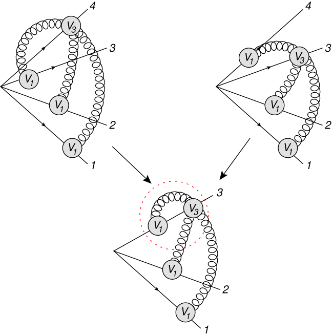
Figure 13: Two different (1,1,1,3)-type webs $w_{1113}(\alpha_{14},\alpha_{24},\alpha_{34})$ (top left) and $w_{1113}(\alpha_{13},\alpha_{23},\alpha_{34})$ (top right), give a contribution to the (1,1,4) web in the limit that lines 3 and 4 are collinear. The red dashed circle indicates the symmetric contribution will be taken.

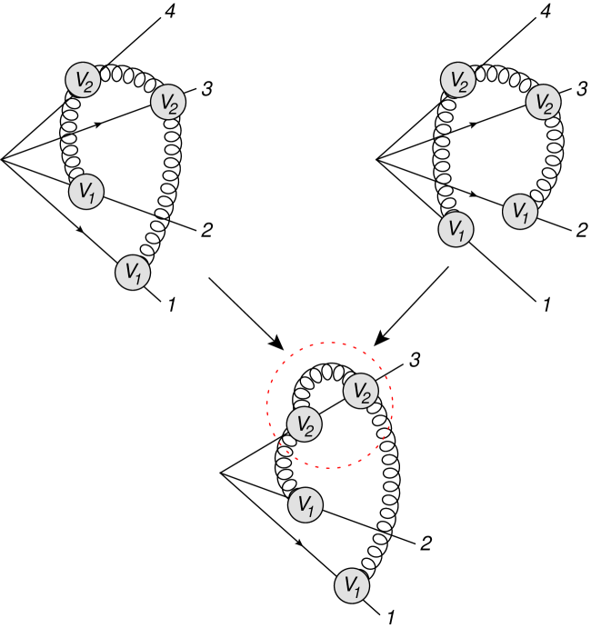
Figure 14: Two different (1,1,2,2) webs $w_{1122}(\alpha_{24},\alpha_{34},\alpha_{13})$ (top left) and $w_{1122}(\alpha_{14},\alpha_{34},\alpha_{23})$ (top right), give a contribution to the (1,1,4) web in the limit that lines 3 and 4 are collinear. The red dashed circle indicates the symmetric contribution regarding the relative position of the two $V_{2}$ vertices along line 3 is taken.

We will now examine taking the limit in more detail. We first note that the collinear limit can only be consistently taken after summing up the four contributions above. Indeed, as we shall see, each of the four separate webs features singularities such as those in eq. (6.1), owing to the fact that $r(\alpha_{ij})$ of eq. (2.45) diverges and the basis functions $M_{k,l,n}(\alpha_{ij})$ become complex in the limit where the would-be-boomerang gluon $\alpha_{ij}\to-1$. We will therefore postpone taking the limit $\alpha_{ij}\to-1$ until we have added all four contributions. Nonetheless, for clarity we consider the four webs in turn.

Let us begin by considering the (1,1,1,3) of figure 15, which is shown in terms of effective vertices in figure 13 (top left).

Figure 15: The (1,1,1,3) web.

According to refs. [44, 45], the integrated subtracted (1,1,1,3) web can be written as

$$\overline{w}^{(3,-1)}_{(1,1,1,3)}\left(\alpha_{14},\alpha_{24},\alpha_{34}\right) = -\frac{1}{6}\,T_{1}^{a}T_{2}^{b}T_{3}^{c}T_{4}^{d}\,\left(\frac{1}{4\pi}\right)^{3}r(\alpha_{14})\,r(\alpha_{24})\,r(\alpha_{34})$$ (6.11)

$$\times\,\Big{[}f^{ade}f^{ebc}\,G_{(1,1,1,3)}\left(\alpha_{14},\alpha_{24},\alpha_{34}\right)+f^{ace}f^{ebd}\,G_{(1,1,1,3)}\left(\alpha_{24},\alpha_{14},\alpha_{34}\right)\Big{]}\,,$$

where

$$\begin{split}&G_{(1,1,1,3)}\left(a_{1},a_{2},a_{3}\right)\,=\,\frac{1}{2}\,M_{2,0,0}(a_{1})M_{0,0,0}(a_{2})M_{0,0,0}(a_{3})\\ &+\,\frac{1}{2}\,M_{2,0,0}(a_{3})M_{0,0,0}(a_{1})M_{0,0,0}(a_{2})-\,M_{2,0,0}(a_{2})M_{0,0,0}(a_{1})M_{0,0,0}(a_{3})\\ &+\,M_{0,0,0}(a_{1})M_{1,0,0}(a_{2})M_{1,0,0}(a_{3})+\,M_{0,0,0}(a_{3})M_{1,0,0}(a_{1})M_{1,0,0}(a_{2})\\ &-\,2\,M_{0,0,0}(a_{2})M_{1,0,0}(a_{1})M_{1,0,0}(a_{3})\,.\end{split}$$ (6.12)

We will now take the collinear limit, beginning with the colour factors. We identify line 4 with line 3 and symmetrise:

$$\begin{split}T_{1}^{a}T_{2}^{b}T_{3}^{c}T_{4}^{d}f^{ade}f^{ebc}\underset{3||4}{\longrightarrow}T_{1}^{a}T_{2}^{b}\frac{1}{2}\{T_{3}^{c},T_{3}^{d}\}f^{ade}f^{ebc}=\frac{1}{2}[T_{1}^{a},T_{1}^{b}][T_{2}^{b},T_{2}^{c}]\{T_{3}^{a},T_{3}^{c}\}=\frac{1}{2}c_{3}^{[3,3]},\\ T_{1}^{a}T_{2}^{b}T_{3}^{c}T_{4}^{d}f^{ace}f^{ebd}\underset{3||4}{\longrightarrow}T_{1}^{a}T_{2}^{b}\frac{1}{2}\{T_{3}^{c},T_{3}^{d}\}f^{ace}f^{ebd}=\frac{1}{2}[T_{1}^{a},T_{1}^{b}][T_{2}^{b},T_{2}^{c}]\{T_{3}^{a},T_{3}^{c}\}=\frac{1}{2}c_{3}^{[3,3]}.\end{split}$$ (6.13)

Identifying lines 3 and 4 in the $\alpha$-variables and defining $\alpha=\alpha_{33}$, we find

$$\begin{split}\overline{w}_{(1,1,1,3)}^{(3,-1)}(\alpha_{14},\alpha_{24},\alpha_{34})\underset{3||4}{\longrightarrow}&-\frac{1}{12}c_{3}^{[3,3]}\left(\frac{1}{4\pi}\right)^{3}r(\alpha_{13})r(\alpha_{23})r(\alpha)\\ &\times\Big{[}G_{(1,1,1,3)}\left(\alpha_{13},\alpha_{23},\alpha\right)+G_{(1,1,1,3)}\left(\alpha_{23},\alpha_{13},\alpha\right)\Big{]}\,,\end{split}$$ (6.14)

where it is understood that the limit $\alpha\to-1$ will be taken once all the contributions are collected.

As shown in figure 13 (top right), we must also consider the (1,1,3,1) web, where three gluons are emitted form line 3. We may readily write the result as $\overline{w}_{(1,1,1,3)}(\alpha_{13},\alpha_{23},\alpha_{34})$ as it corresponds to the (1,1,1,3) web considered above with lines 3 and 4 swapped. Repeating the steps above yields

$$\begin{split}\overline{w}_{(1,1,3,1)}^{(3,-1)}(\alpha_{13},\alpha_{23},\alpha_{34})\underset{3||4}{\longrightarrow}&-\frac{1}{12}c_{3}^{[3,3]}\left(\frac{1}{4\pi}\right)^{3}r(\alpha_{13})r(\alpha_{23})r(\alpha)\\ &\times\Big{[}G_{(1,1,1,3)}\left(\alpha_{13},\alpha_{23},\alpha\right)+G_{(1,1,1,3)}\left(\alpha_{23},\alpha_{13},\alpha\right)\Big{]},\end{split}$$ (6.15)

which is the same contribution as eq. (6.14).

Figure 16: The (1,1,2,2) web.

Next, we must consider the (1,1,2,2) web of figure 16, shown with effective vertices in figure 14, top-left. The subtracted web is given by a permutation of the (1,2,2,1) web [44, 45]:

$$\overline{w}^{(3,-1)}_{(1,1,2,2)}\left(\alpha_{14},\alpha_{34},\alpha_{23}\right) = \frac{1}{6}\,f^{ade}f^{ebc}T_{1}^{a}T_{2}^{b}T_{3}^{c}T_{4}^{d}\,\,\left(\frac{1}{4\pi}\right)^{3}r(\alpha_{12})\,r(\alpha_{23})\,r(\alpha_{34})$$ (6.16)

$$\hskip 56.9055pt\times\,G_{(1,1,2,2)}\left(\alpha_{14},\alpha_{34},\alpha_{23}\right)\,,$$

where

$$\begin{split}&G_{(1,1,2,2)}\left(a_{1},a_{2},a_{3}\right)\,=\,-\,\frac{1}{2}\,M_{2,0,0}(a_{1})M_{0,0,0}(a_{2})M_{0,0,0}(a_{3})\\ &-\,\frac{1}{2}\,M_{2,0,0}(a_{3})M_{0,0,0}(a_{1})M_{0,0,0}(a_{2})+M_{2,0,0}(a_{2})M_{0,0,0}(a_{1})M_{0,0,0}(a_{3})\\ &-\,M_{0,0,0}(a_{1})M_{1,0,0}(a_{2})M_{1,0,0}(a_{3})-M_{0,0,0}(a_{3})M_{1,0,0}(a_{1})M_{1,0,0}(a_{2})\\ &+\,2\,M_{0,0,0}(a_{2})M_{1,0,0}(a_{1})M_{1,0,0}(a_{3})-4\,M_{0,2,0}(a_{2})M_{0,0,0}(a_{1})M_{0,0,0}(a_{3})\,.\end{split}$$ (6.17)

Note the second argument in this function, $a_{2}$, corresponds to the $\alpha$ between the two lines with two gluons attached; this is the gluon which is due to become a boomerang. The result is symmetric between $a_{1}$ and $a_{3}$. Using eq. (6.13), we find

$$\begin{split}\overline{w}_{(1,1,2,2)}^{(3,-1)}(\alpha_{14},\alpha_{34},\alpha_{23})\underset{3||4}{\longrightarrow}&\,\,\frac{1}{12}c_{3}^{[3,3]}\left(\frac{1}{4\pi}\right)^{3}r(\alpha_{13})r(\alpha_{23})r(\alpha)G_{(1,1,2,2)}\left(\alpha_{13},\alpha,\alpha_{23}\right).\end{split}$$ (6.18)

The second (1,1,2,2) web is a different permutation of the (1,2,2,1) web in refs. [44, 45] which corresponds to $\overline{w}_{1122}(\alpha_{13},\alpha_{34},\alpha_{24})$ (figure 14). Repeating the steps above gives

$$\begin{split}\overline{w}_{(1,1,2,2)}^{(3,-1)}(\alpha_{13},\alpha_{34},\alpha_{24})\underset{3||4}{\longrightarrow}&\,\,\frac{1}{12}c_{3}^{[3,3]}\left(\frac{1}{4\pi}\right)^{3}r(\alpha_{13})r(\alpha_{23})r(\alpha)G_{(1,1,2,2)}\left(\alpha_{13},\alpha,\alpha_{23}\right).\end{split}$$ (6.19)

Finally, the (1,1,4) web should be obtained by 1/2 the sum of the four contributions in eqs. (6.14), (6.15), (6.18) and (6.19). The factor of 1/2 is due following step 4 in the rules at the start of this section, reflecting the fact that the (1,1,4) web has higher symmetry than the original webs, since the ends of the boomerang gluon now attach to the same Wilson line. The collinear reduction procedure thus gives

$$\begin{split}\overline{w}^{(3,-1)}_{(1,1,4);3}=\,&\frac{1}{2}\,\lim_{3||4}\Bigg{\{}\overline{w}^{(3,-1)}_{(1,1,1,3)}\left(\alpha_{14},\alpha_{24},\alpha_{34}\right)+\overline{w}_{(1,1,3,1)}^{(3,-1)}(\alpha_{13},\alpha_{23},\alpha_{34})\\ &\hskip 50.0pt+\overline{w}_{(1,1,2,2)}^{(3,-1)}(\alpha_{14},\alpha_{34},\alpha_{23})+\overline{w}_{(1,1,2,2)}^{(3,-1)}(\alpha_{13},\alpha_{34},\alpha_{24})\Bigg{\}}\\ =\,&\frac{1}{2}\,\lim_{\alpha\to-1}\Bigg{\{}-\frac{1}{6}c_{3}^{[3,3]}\left(\frac{1}{4\pi}\right)^{3}r(\alpha_{13})r(\alpha_{23})r(\alpha)\\ &\qquad\qquad\times\Big{[}G_{(1,1,1,3)}\left(\alpha_{13},\alpha_{23},\alpha\right)+G_{(1,1,1,3)}\left(\alpha_{23},\alpha_{13},\alpha\right)-G_{(1,1,2,2)}\left(\alpha_{13},\alpha,\alpha_{23}\right)\Big{]}\Bigg{\}}\\ =\,&\frac{1}{2}\,\lim_{\alpha\to-1}\left\{-\frac{2}{3}c_{3}^{[3,3]}\left(\frac{1}{4\pi}\right)^{3}r(\alpha_{13})r(\alpha_{23})r(\alpha)M_{0,0,0}(\alpha_{13})M_{000}(\alpha_{23})M_{0,2,0}(\alpha)\right\}\\ =\,&-c_{3}^{[3,3]}\left(\frac{1}{4\pi}\right)^{3}\frac{4\pi^{2}}{9}r(\alpha_{13})r(\alpha_{23})M_{0,0,0}(\alpha_{13})M_{0,0,0}(\alpha_{23})\,,\end{split}$$ (6.20)

where in the second step we inserted the expressions for the kinematic functions $G_{(1,1,1,3)}$ and $G_{(1,1,2,2)}$ from eqs. (6.12) and (6.17) in terms of basis functions, observing a remarkable cancellation of all terms except for the one containing $M_{0,2,0}(\alpha)$, and in the last step we have taken the limit $\alpha\to-1$, using

$$\lim_{\alpha\to-1}r(\alpha)\,M_{0,2,0}(\alpha)=\lim_{\alpha\to-1}\frac{1+\alpha^{2}}{1-\alpha^{2}}\left(\frac{2}{3}\log^{3}(\alpha)+4\zeta_{2}\ln(\alpha)\right)=\frac{4}{3}\pi^{2}\,.$$ (6.21)

Note that the two terms in the brackets conspire to cancel the singularity, yielding together a finite, real limit.

In summary we observe here multiple cancellations of potential singularities emanating from the pole of $r(\alpha)$, which is realised in the sum of webs in eq. (6.20) both through the cancellation of a host of terms containing the basis functions $M_{0,0,0}(\alpha)$, $M_{1,0,0}(\alpha)$ and $M_{2,0,0}(\alpha)$ and through the finite limit of the remaining $r(\alpha)M_{0,2,0}(\alpha)$ term. The final result in eq. (6.20) exactly matches the $c_{3}^{[3,3]}$ contribution to the (1,1,4) web of eq. (5.11) obtained by a direct computation (see appendix E, with the result given in eq. (E.15) there).

As already discussed above, it is not possible to reproduce the fully antisymmetric colour factor $c_{4}^{[3,3]}$ by collinear reduction. Thus, this contribution to the (1,1,4) web cannot be checked by this procedure. Furthermore, the (1,2,3) boomerang web – which only has a $c_{4}^{[3,3]}$ term – is also unobtainable.

Next, let us consider the two-line webs of section 5.2. Of the three boomerang-web examples considered there, the (3,3), (5,1) and (2,4), only the last has a component that is accessible through collinear reduction, namely its contribution involving the $c_{2}^{[3,2]}$ colour factor of eq. (5.25), which involves anticommutators. All other contributions of these two-line webs are proportional to $c_{1}^{[3,2]}$ and are thus unobtainable through collinear reduction.

The $c_{2}^{[3,2]}$ contribution to the (2,4) web was computed directly in eq. (5.68). Using the notation of eq. (2.22) and the basis functions in appendix B, the result can be expressed as:

$$\overline{w}^{(3,-1)}_{(2,4);2}(\alpha_{13})=\,\left(\frac{1}{4\pi}\right)^{3}\,c_{2}^{[3,2]}F^{(3)}_{(2,4);2}(\alpha_{13})\,=-\left(\frac{1}{4\pi}\right)^{3}\,c_{2}^{[3,2]}\,\frac{4}{9}\pi^{2}\Big{(}r(\alpha_{13})M_{0,0,0}(\alpha_{13})\Big{)}^{2}\,,$$ (6.22)

where the colour factor is defined in eq. (5.25) and for later convenience we renamed the Wilson lines as 1 and 3.

Let us now compare this to the collinear reduction of the (1,1,4) web, i.e. starting with the final result in eq. (6.20) and considering the limit $1||2$. Let us first examine the colour factor $c_{3}^{[3,3]}$ defined in eq. (5.1). We find that upon merging the lines 1 and 2, it becomes

$$c_{3}^{[3,3]}=-f^{cbe}f^{ade}T_{1}^{a}T_{2}^{b}T_{3}^{\{c,d\}}\,\to\,-f^{cbe}f^{ade}\frac{1}{2}T_{1}^{\{a,b\}}T_{3}^{\{c,d\}}=2c_{2}^{[3,2]}\,,$$ (6.23)

where in the final step we used the definition in eq. (5.25). Upon applying collinear reduction to the (1,1,4) web of eq. (6.20) we must account for the extra symmetry of the (2,4) web due to the fact that the two non-boomerang gluons connect the same two Wilson lines (but distinct lines in the original (1,1,4) web) by including an extra factor $1/2$. We thus obtain,

$$\begin{split}\overline{w}^{(3,-1)}_{(2,4);2}(\alpha_{13})\,&=\,\frac{1}{2}\lim_{1||2}\overline{w}^{(3,-1)}_{(1,1,4);3}(\alpha_{13},\alpha_{23})\\ \,&=\,\frac{1}{2}\lim_{1||2}\Bigg{\{}-c_{3}^{[3,3]}\left(\frac{1}{4\pi}\right)^{3}\frac{4\pi^{2}}{9}r(\alpha_{13})r(\alpha_{23})M_{0,0,0}(\alpha_{13})M_{0,0,0}(\alpha_{23})\Bigg{\}}\,\\ \,&=\,-c_{2}^{[3,2]}\left(\frac{1}{4\pi}\right)^{3}\frac{4\pi^{2}}{9}\Big{(}r(\alpha_{13})M_{0,0,0}(\alpha_{13})\Big{)}^{2}\,,\end{split}$$ (6.24)

where in the final step we just used the reduced colour structure from eq. (6.23) and identified $\alpha_{23}=\alpha_{13}$. In this case, no $\alpha$ variable tends to $-1$, as no new boomerang gluon is generated, so the limit is straightforward to take. Evidently eq. (6.24) agrees with the direct computation in eq. (6.22), thus providing an additional check of the computations.

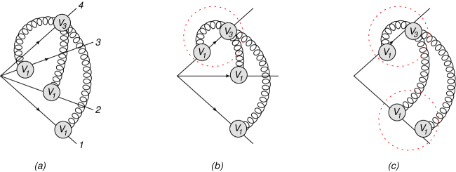
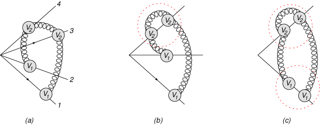
Figure 17: Upper diagrams: (a) Effective vertex diagram for the (1,1,1,3) web; (b) Contribution to the (1,1,4) web obtained from collinear reduction of (a); (c) Contribution to the (2,4) web obtained from collinear reduction of (b). The red circle denotes symmetrisation of vertices. Lower diagrams: The same starting with the 1122 web.

To conclude this section it is useful to take another look at the collinear reduction process we have just completed, in which two consecutive collinear limits have been applied, first getting the $c_{3}^{[3,3]}$ component of the (1,1,4) web by taking $3||4$, and then getting the $c_{2}^{[3,2]}$ component of the (2,4) web by further taking $1||2$. This process is summarised diagrammatically in figure 17 using the effective vertex formalism. The basic feature of this example of collinear reduction, is what is described by eq. (6.10), namely that the very same colour structure of three-line webs emerges upon merging different configurations of effective vertices. Of course the same follows for the two-line colour structure $c^{[3,2]}_{2}$, which can be expressed in two different ways as

$$c^{[3,2]}_{2} =-\frac{1}{4}\left\{T_{1}^{a},T_{1}^{b}\right\}\left\{T_{3}^{c},\,C_{3,2}^{ac,b}(3)\right\}\,,$$ (6.25a)

$$c^{[3,2]}_{2} =\frac{1}{4}\left\{T_{1}^{a},T_{1}^{b}\right\}\left\{C_{2,1}^{be}(3),\,C_{2,1}^{ea}(3)\right\}\,.$$ (6.25b)

This interesting example therefore illustrates both the over-completeness of the colour basis of eq. (2.26) when used to express boomerang webs and the non-trivial structure of the relations between webs spanning a different number of Wilson lines.

7 Discussion

In this paper, we have have taken another step towards the calculation of the multiparton soft anomalous dimension for massive Wilson lines at three-loop order, continuing the programme of work developed in refs. [55, 57, 58, 44, 45]. In our approach, the logarithm of the soft function is calculated directly in terms of Feynman diagrams known as (multiparton) webs. In this work we have focused specifically on what we call boomerang webs, containing multiple gluon exchanges where at least one gluon has both its endpoints on the same Wilson line. As in previous work on Multiple Gluon Expchange Webs (MGEWs), we set up the calculation in configuration space, and introduced a suitable exponential infrared regulator in order to isolate the ultraviolet divergences associated with the vertex where the Wilson lines meet. The latter are evaluated using dimensional regularization. We have classified all boomerang webs through three-loop order, addressed new aspects of regularization and renormalization that arise in this class of webs and provided explicit results for their contributions to the soft anomalous dimension.

Beyond the significance of the results as components of the three-loop massive soft anomalous dimension, our study highlights several interesting aspects of webs and multi-loop computations. First, we find that self-energy diagrams, including arbitrary clusters of such, completely decouple from other boomerang webs. Boomerang webs which span two or more Wilson lines, include a priori both self-energy subdiagrams and diagrams where the boomerang gluons straddle one or more emission vertices connecting to other Wilson lines. However, we have proven in full generality (section 4) that only the latter type contribute. That is, all web diagrams containing self-energy subdiagrams have a vanishing exponentiated colour factor. This clearly simplifies the computation of such webs, since only a subset of the diagrams need to be computed. Furthermore, the boomerang gluons in these diagrams do not require any infrared regulator: their regularization is guaranteed by that associated with the non-boomerang gluons which they straddle. This is shown in section 3.3 and illustrated in a variety of examples in section 5.

Our proof for the complete decoupling of self-energy diagrams from multi-line boomerang webs utilises the replica trick and relies on the combinatorial properties of the web mixing matrix, as well as the colour algebra (namely that self-energy-type subdiagrams are diagonal in colour space). These general observations suggest that there may be further interesting insights to be gained about the structure of web mixing matrices, and also about what happens when one combines their combinatorial properties with the known colour algebra of a non-Abelian gauge theory. Recently, the calculation of these matrices was systematically extended to the four-loop order [65, 66], so there is clear scope for further progress in this area.

A significant part of our study here has been dedicated to the properties of the kinematic functions arising in boomerang webs. Our findings are consistent with the conjecture [45, 44] that MGEWs spanning several Wilson lines are expressible as sums of products of harmonic polylogarithms of individual cusp angles $\alpha_{ij}$, multiplied by a unique rational function $r(\alpha_{ij})=\frac{1+\alpha_{ij}^{2}}{1-\alpha_{ij}^{2}}$ for every gluon exchange between the lines $i$ and $j$. As reviewed in section 2.4, the appearance of these functions can be most easily understood in configuration space, where a suitable choice of variables leads to factorization of the gluon propagator, and the integral can be recast in a $d\log$ form. This was first noted in the context of the angle-dependent cusp anomalous dimension [70], and then conjectured to apply to any MGEW [45, 44]. The fact that the dependence on several kinematic variables does not lead to new types of singularities is a highly non-trivial feature, which is special to MGEWs. Moreover, as reviewed here in section 2.5, MGEWs were conjectured to be expressible in terms of a restricted class of harmonic polylogarithms, defined (see eq. (2.50)) through a single integral over a product of three types of logarithms [45]. In this paper we extended the class of webs for which this conjecture was tested. We found that while the main properties still hold, namely boomerang webs are still expressible as sums of products of the same basis of functions, one salient feature is lost, namely boomerang webs are no more functions of uniform, maximal transcendental weight. Instead, they always display a weight-drop of at least one unit for every boomerang gluon (with no rational factor) and furthermore, often feature mixed weight, as summarised in Table 2.

The mechanism leading to the weight-drop and the mixed weight is analysed in some detail in section 3.3. This may be of broader interest, well beyond the context of webs, because a general understanding of transcendental weight in perturbative computations is lacking. In particular, while it has been observed that certain quantities in ${\cal N}=4$ Super-Yang-Mills (SYM) feature uniform, maximal weight, and moreover are equal to the maximal weight terms on the corresponding quantities in QCD, these properties are not general, and the underlying mathematical reasons for these relations and for the complex mixed-weight structure in QCD, remain elusive. Nevertheless, from the perspective of comparing results in different gauge theories it is not surprising to see that non-boomerang MGEWs have uniform maximal weight, while boomerang webs feature a weight-drop and mixed weight. Indeed, only the latter contribute to the renormalization of the coupling, thus affecting the QCD result, while not the ${\cal N}=4$ SYM one.

Our finding that, despite the mixed weight, boomerang webs can still be expressed in terms of the same basis of functions provides further evidence that the conjecture above holds for all MGEWs. This is interesting because it is already known that going beyond MGEWs, the basis of transcendental functions must be extended (and likewise the set of rational functions they accompany) as seen explicitly in the calculation of the angle-dependent cusp anomalous dimension in QCD at three loops [9, 8], and in QED [10] at four loops.

In section 6, we have generalised and applied the collinear reduction procedure developed in ref. [45], motivated by the effective vertex formalism of ref. [58]. First we have seen that collinear limits generating boomerang gluons involve taking the limit $\alpha_{ij}\to-1$, which may be rather subtle in dimensional regularization. For the self-energy web, the direct computation requires $\epsilon>\frac{1}{2}$, and it therefore cannot be recovered from the expanded (1,1) web. We have then seen that in boomerang webs, in which boomerang gluons straddle other emissions along the Wilson line, order-by-order treatment in $\epsilon$ is in fact possible, as all singularities are regularised by small positive values of $\epsilon$. This guarantees the validity in principle of the collinear reduction process.

Next we examined the non-trivial example of the (1,1,4) web, demonstrating that it can be recovered from results for non-boomerang four-line webs. Specifically, we have shown that upon considering the complete set of four-line webs (specifically, the (1,1,1,3), (1,1,3,1) webs and two instances of the (1,1,2,2) web) whose collinear limit contribute to the (1,1,4) web, the limit exists, and through a rather intricate set of cancellations, reproduces the result of the direct calculation. This provides a strong check of our results.

The fact that different four-line webs, with different compositions of effective colour vertices contribute together is an interesting feature, which is a reflection of the fact that the basis in eq. (2.26) becomes over-complete when contracting pairs of adjoint indices of different effective colour vertices on the same line, as needed when forming boomerang webs. While we showed that collinear reduction may be used to compute (or check) certain components of boomerang webs, we stress that this procedure does not constrain those contributions to lower-line webs involving a fully antisymmetric colour factor, such as e.g. $c_{4}^{[3,3]}$ in eq. (5.1) or $c_{1}^{[3,2]}$ in eq. (5.25), and thus cannot be generally used as a replacement of direct computations.

Work towards calculating the remaining contributions to the soft anomalous dimension is ongoing, using a range of different techniques. In this paper, we have completed another subset of the remaining calculations while also proving a general result on the decoupling of self-energy diagrams and deepening our understanding of the analytic structure of webs and their collinear limits.

Appendix A Results for lower-order webs

Here, we collect some useful results for one- and two-loop webs, obtained in refs. [44, 45] using the approach described in section 2. First, there is the single gluon exchange web connecting lines $i$ and $j$ at one-loop order. This web has a colour factor $c^{[1,2]}=T_{1}\cdot T_{2}$ and a kinematic factor

$$\begin{split}\mathcal{F}^{(1)}(\alpha_{12},\mu^{2}/m^{2},\epsilon)\,&=\,\kappa\Gamma(2\epsilon)\int_{0}^{1}dxp_{\epsilon}(x,\alpha_{12})\\ \,&=\,\kappa\Gamma(2\epsilon)\,\frac{r(\alpha_{12})}{\epsilon}\left({}_{2}F_{1}\left(1,2\epsilon,1+\epsilon,\frac{\alpha_{12}}{1+\alpha_{12}}\right)-{}_{2}F_{1}\left(1,2\epsilon,1+\epsilon,\frac{1}{1+\alpha_{12}}\right)\right)\\ \,&=\,\kappa\Gamma(2\epsilon)\,2r(\alpha_{12})\ln(\alpha_{12})+\,{\cal O}(\epsilon^{0})\,\\ \,&=\,-\frac{g_{s}^{2}}{16\pi^{2}}\,\frac{2}{\epsilon}\,r(\alpha_{12})\,\ln(\alpha_{12})\,+\,{\cal O}(\epsilon^{0})\,,\end{split}$$ (A.1)

where in the first line we used $p_{\epsilon}(x,\alpha)$ of eq. (2.42), in the second we performed the integral keeping the exact $\epsilon$ dependence in terms of Gauss hypergeometric functions, and expressed the rational function using $r(\alpha)$ of eq. (2.45) and in the third and fourth lines we expanded in $\epsilon$ keeping only the singular term. Higher-order terms, ${\cal O}(\epsilon^{k})$ for $k\geq 0$, will be needed for the renormalization of higher-order webs. These follow simply from expansion of the propagator function $p_{\epsilon}$ under the integral in the first line of (A.1) according to eq. (2.43), or alternatively from the $\epsilon$ expansion of the hypergeometric functions in the second line of eq. (A.1).

Next, consider the two-loop three-line (1,1,2) web of figure 18.

Figure 18: The (1,1,2) web.

This web contributes through a single connected colour factor proportional to the structure constant $f^{abc}$. Considering a (1,1,2) web with two attachments on line $3$ and single attachments on each of the lines $1$ and $2$, the colour factor is $c^{[2,3]}=\frac{1}{2}if^{abc}T_{1}^{a}T_{2}^{b}T_{3}^{c}$ and the corresponding kinematic factor (for the non-subtracted web) is (see ref. [44])

$$\begin{split}\mathcal{F}_{(1,1,2)}^{(2)}(\alpha_{13},\alpha_{23})&=\kappa^{2}\Gamma(4\epsilon)\frac{1}{2\epsilon}\int_{0}^{1}dydz\,p_{\epsilon}(y,\alpha_{23})p_{\epsilon}(z,\alpha_{13})\\ &\qquad\left\{\left(\frac{z}{y}\right)^{2\epsilon}{{}_{2}}F_{1}\left(4\epsilon,2\epsilon;1+2\epsilon;-\frac{z}{y}\right)-\left(\frac{y}{z}\right)^{2\epsilon}{{}_{2}}F_{1}\left(4\epsilon,2\epsilon;1+2\epsilon;-\frac{y}{z}\right)\right\}\\ &=2\kappa^{2}\Gamma(4\epsilon)\int_{0}^{1}dydz\,p_{\epsilon}(z,\alpha_{13})p_{\epsilon}(y,\alpha_{23})\Big{[}\ln\left(\frac{z}{y}\right)+\,\epsilon\,\Big{\{}4\text{Li}_{2}\left(-\frac{z}{y}\right)\\ &\quad+\ln^{2}\left(\frac{z}{y}\right)+\frac{\pi^{2}}{3}\Big{\}}+\mathcal{O}(\epsilon^{2})\Big{]}.\end{split}$$ (A.2)

Finally, let us consider the two-loop two-line web consisting of two gluons exchanged between lines $1$ and $2$. This web has two diagrams, but only one of them, with the gluons crossed (see figure 19), has a non-vanishing exponentiated colour factor $c^{[2,2]}=\frac{N_{c}}{2}\,T_{1}\cdot T_{2}$. The corresponding kinematic factor was computed long ago [7]. In our notations it is reported in eq. (4.7) in [45] and it reads:

$$\mathcal{F}^{(2,-1)}_{X}=\kappa^{2}\Gamma(4\epsilon)\int_{0}^{1}dy\,dz\,p_{0}(y,\alpha_{12})p_{0}(z,\alpha_{12})\text{ln}\Big{(}\frac{1-z}{1-y}\frac{y}{z}\Big{)}\theta(y>z),$$ (A.3)

at ${\cal O}(\epsilon^{-1})$ and

$$\begin{split}\mathcal{F}^{(2,0)}_{X}&=\kappa^{2}\Gamma(4\epsilon)\int_{0}^{1}dydz\,p_{0}(y,\alpha_{12})p_{0}(z,\alpha_{12})\Big{[}\text{ln}^{2}\Big{(}\frac{1-z}{1-y}\Big{)}-\text{ln}^{2}\Big{(}\frac{z}{y}\Big{)}-4\,\text{Li}_{2}\Big{(}-\frac{z}{y}\Big{)}\\ &+4\text{Li}_{2}\Big{(}-\frac{1-z}{1-y}\Big{)}+\text{ln}\Big{(}\frac{1-z}{1-y}\frac{y}{z}\Big{)}\text{ln}\big{(}q(y,\alpha_{12})q(z,\alpha_{12})\big{)}\Big{]}\theta(y>z).\end{split}$$ (A.4)

and ${\cal O}(\epsilon^{0})$.

Figure 19: The (2,2) web: the crossed-gluon diagram denoted by $X$ in the text is the only diagram in the (2,2) web with a non-zero exponentiated colour factor.

Appendix B Basis functions and their symbols

In this appendix, we present explicit forms for the basis functions of eq. (2.50), together with their symbols, as taken from ref. [45]. We only include the functions up to weight 4, as higher-weights do not appear in the webs computed here at ${\cal O}(1/\epsilon)$. We refer the reader to ref. [45] for a more complete list.

For the functions themselves, we have

• Weight one.

  $$\begin{split}M_{0,0,0}(\alpha)\,=\,2\log(\alpha)\,.\end{split}$$ (B.1)

• Weight two.

  $$\begin{split}M_{1,0,0}(\alpha)\,=\,2\,\text{Li}_{2}(\alpha^{2})+4\log(\alpha)\log\left(1-\alpha^{2}\right)-2\log^{2}(\alpha)-2\,\zeta_{2}.\end{split}$$ (B.2)

• Weight three.

  $$\begin{split}M_{0,0,2}(\alpha)\,=\,\frac{8}{3}\log^{3}(\alpha)\,,\end{split}$$ (B.3)

  $$\begin{split}M_{0,1,1}(\alpha)\,=\,2\,\text{Li}_{3}(\alpha^{2})-2\log(\alpha)\bigg{[}\text{Li}_{2}(\alpha^{2})+\frac{\log^{2}(\alpha)}{3}+\zeta_{2}\bigg{]}-2\,\zeta_{3}\,,\end{split}$$ (B.4)

  $$\begin{split}M_{0,2,0}(\alpha)\,=\,\frac{2}{3}\log^{3}(\alpha)+4\,\zeta_{2}\,\log(\alpha)\,,\end{split}$$ (B.5)

  $$\begin{split}M_{2,0,0}(\alpha)&=-\,4\,\bigg{[}\text{Li}_{3}(\alpha^{2})+2\text{Li}_{3}\left(1-\alpha^{2}\right)\bigg{]}-8\log\left(1-\alpha^{2}\right)\log^{2}(\alpha)\\ &+\,\frac{8}{3}\,\log^{3}(\alpha)+8\,\zeta_{2}\,\log(\alpha)+4\,\zeta_{3}\,.\end{split}$$ (B.6)

• Weight four.

  $$\begin{split}M_{3,0,0}(\alpha)&=\,12\,\bigg{[}\text{Li}_{4}(\alpha^{2})-4\,\text{Li}_{4}\left(1-\alpha^{2}\right)\bigg{]}-24\,S_{2,2}(\alpha^{2})\\ &-\,24\,\log\left(1-\alpha^{2}\right)\,\text{Li}_{3}(\alpha^{2})-24\,\log^{2}\left(1-\alpha^{2}\right)\,\log^{2}(\alpha)\\ &+\,16\,\log\left(1-\alpha^{2}\right)\,\log^{3}(\alpha)-\,4\,\log^{4}(\alpha)\\ &-\,24\,\zeta_{2}\,\log(\alpha)\,\log\left[\frac{\alpha}{\left(1-\alpha^{2}\right)^{2}}\right]\\ &+\,24\,\zeta_{3}\,\log\left[\alpha\left(1-\alpha^{2}\right)\right]-\,6\,\zeta_{4}\,,\end{split}$$ (B.7)

  $$\begin{split}M_{1,2,0}(\alpha)&=\,4\,\text{Li}_{4}(\alpha^{2})-4\,\log(\alpha)\,\text{Li}_{3}(\alpha^{2})+2\,\log^{2}(\alpha)\,\text{Li}_{2}(\alpha^{2})\\ &+\,\frac{4}{3}\,\log^{3}(\alpha)\,\log\left(1-\alpha^{2}\right)-\,\frac{2}{3}\,\log^{4}(\alpha)\\ &+\,\zeta_{2}\,\Big{[}8\,\log(\alpha)\log\left(1-\alpha^{2}\right)+4\,\text{Li}_{2}(\alpha^{2})-6\,\log^{2}(\alpha)\Big{]}\\ &+\,4\,\zeta_{3}\,\log(\alpha)-14\,\zeta_{4}\,,\end{split}$$ (B.8)

  $$\begin{split}M_{1,0,2}(\alpha)&=\,4\,\text{Li}_{4}(\alpha^{2})-8\,\log(\alpha)\,\text{Li}_{3}(\alpha^{2})+8\,\log^{2}(\alpha)\,\text{Li}_{2}(\alpha^{2})\\ &+\frac{16}{3}\,\log^{3}(\alpha)\,\log\left(1-\alpha^{2}\right)-\,\frac{4}{3}\,\log^{4}(\alpha)-4\,\zeta_{4}\,,\end{split}$$ (B.9)

  $$\begin{split}M_{1,1,1}(\alpha)&=-\,4\,\text{Li}_{4}(\alpha^{2})+4\,S_{2,2}(\alpha^{2})+2\,\log\left[\alpha\left(1-\alpha^{2}\right)^{2}\right]\,\text{Li}_{3}(\alpha^{2})\\ &+\,4\,\log(\alpha)\,\text{Li}_{3}\left(1-\alpha^{2}\right)\\ &-\,\frac{4}{3}\,\log^{2}(\alpha)\,\log\left(1-\alpha^{2}\right)\bigg{[}\log(\alpha)-3\,\log\left(1-\alpha^{2}\right)\bigg{]}\\ &-\,8\,\zeta_{2}\,\log(\alpha)\log(1-\alpha^{2})-2\,\zeta_{3}\,\log\left[\alpha\left(1-\alpha^{2}\right)^{2}\right]+3\,\zeta_{4}\,,\end{split}$$ (B.10)

  $$M_{0,2,1}(\alpha) =\frac{2}{3}\pi^{2}\log^{2}(\alpha)+\frac{2}{3}\log^{4}(\alpha)\,,$$ (B.11)

  $$M_{0,0,3}(\alpha) =4\log^{4}(\alpha)\,.$$ (B.12)

One can easily check that

$$M_{0,2,1}(\alpha)=\frac{1}{2}M_{0,0,0}(\alpha)M_{0,2,0}(\alpha)$$ (B.13)

which is one example of the relations in eq. (2.51). The symbol of each function may be found in table 3.

$M_{k,l,n}(\alpha)$
w	Name	symbol
1	$M_{0,0,0}$	$2\,(\otimes\alpha)$
2	$M_{1,0,0}$	$-4\,\alpha\otimes\eta$
3	$M_{0,0,2}$	$16\,\alpha\otimes\alpha\otimes\alpha$
	$M_{0,1,1}$	$-4\,\alpha\otimes\eta\otimes\alpha$
	$M_{0,2,0}$	$4\,\alpha\otimes\alpha\otimes\alpha$
	$M_{2,0,0}$	$16\,\alpha\otimes\eta\otimes\eta$
4	$M_{1,0,2}$	$-32\,\alpha\otimes\alpha\otimes\alpha\otimes\eta$
	$M_{1,1,1}$	$-16\,\alpha\otimes\alpha\otimes\alpha\otimes\alpha+8\,\alpha\otimes\eta\otimes\alpha\otimes\eta+8\,\alpha\otimes\eta\otimes\eta\otimes\alpha$
	$M_{1,2,0}$	$-8\,\alpha\otimes\alpha\otimes\alpha\otimes\eta-8\,\alpha\otimes\eta\otimes\alpha\otimes\alpha$
	$M_{3,0,0}$	$-96\,\alpha\otimes\eta\otimes\eta\otimes\eta$
	$M_{0,2,1}$	$16\,\alpha\otimes\alpha\otimes\alpha\otimes\alpha$
	$M_{0,0,3}$	$96\,\alpha\otimes\alpha\otimes\alpha\otimes\alpha$

Table 3: Symbols of the all linearly independent functions of the MGEW basis of eq. (2.50) up to weight $4$.

Appendix C Gluon emission vertex counterterm

In this appendix, we calculate the counterterm for the vertex coupling a gluon to a Wilson line. Consider the diagram of figure 20, which shows a gluon being emitted from a Wilson line at distance parameter $u$, dressed by a boomerang gluon whose endpoints have distances $s$ and $t$. To identify the singularity associated with the boomerang gluon we must integrate over $s$ and $t$, keeping $u$ fixed.

Figure 20: Diagram used for the calculation of the vertex counterterm, where $\beta$ is the 4-velocity of the Wilson line, and $\mu$ the Lorentz index of the emitted gluon.

Applying the Feynman rules of eqs. (2.27, 2.29), but removing the exponential regulator for the boomerang gluon as discussed in section 3.2, we obtain

$$ig_{s}\,\mu^{\epsilon}\,T_{1}^{b}T_{1}^{a}T_{1}^{b}\beta^{\mu}\int_{0}^{\infty}due^{-imu\sqrt{\beta^{2}-i\varepsilon}}I(u),$$ (C.1)

where

$$I(u) ={\cal N}g_{s}^{2}\mu^{2\epsilon}\,\beta^{2}\int_{0}^{u}ds\int_{u}^{\infty}dt\left[-(t\beta-s\beta)^{2}\right]^{\epsilon-1}$$

$$=-{\cal N}g_{s}^{2}\mu^{2\epsilon}\,(-\beta^{2})^{\epsilon}\int_{0}^{u}ds\int_{u}^{\infty}dt\,(t-s)^{2\epsilon-2}$$

$$=-{\cal N}g_{s}^{2}\mu^{2\epsilon}\,(-\beta^{2})^{\epsilon}u^{2\epsilon}\frac{1}{2\epsilon\,(1-2\epsilon)}\,,$$ (C.2)

where in the last line we performed the integrals over $s$ and $t$ assuming $0<\epsilon<\frac{1}{2}$. We conclude that upon neglecting terms of ${\cal O}(\epsilon^{0})$ and above, eq. (C.1) assumes the form of a usual emission vertex from a Wilson line, multiplied by the factor

$$-\frac{g_{s}^{2}}{8\pi^{2}\epsilon}\,\left(C_{R_{1}}-\frac{1}{2}N_{c}\right)+{\cal O}(\epsilon^{0})\,,$$ (C.3)

where we manipulated the colour factor in eq. (C.1) as in eq. (3.6). Equation (C.3) represents the singularity associated with shrinking the boomerang gluon surrounding the emission vertex to a point. To remove this local singularity, we must introduce a pure counterterm that is the negative of this result, i.e.

$$Z_{v}=1+Z_{v}^{(1)}\left(C_{R_{1}}-\frac{1}{2}N_{c}\right)+\ldots\,,\qquad\quad Z_{v}^{(1)}=+\frac{g_{s}^{2}}{8\pi^{2}\epsilon}\,\,\,,$$ (C.4)

where the subscript $v$ stands for the gluon-emission vertex.

Appendix D Calculation of web mixing matrices

In this appendix we review the replica-trick based algorithm developed in ref. [55] for calculating the web mixing matrix of eq. (2.14) for a given web. This algorithm is also heavily used in section 4 to prove that self-energy graphs do not contribute in the overall expression for a boomerang web.

Given a web $W$, we may separate its soft gluon part (i.e. the part of the diagrams remaining after the Wilson lines are removed) into a set of $n_{c}$ connected pieces. We now consider a theory in which there are $N$ non-interacting copies of the gluon fields, which may connect with the same Wilson lines. Then one may associate a replica index $i\in[1,N]$ with each connected subdiagram, such that these are completely independent. The exponentiated colour factor of eq. (4.1) for a given diagram $D$ is then obtained as follows:

1. One considers a particular hierarchy $h$ of the $n_{c}$ replica number assignments for all connected pieces of $D$.

2. For each $h$, one reorders the gluon attachments on each Wilson line, so that replica indices are increasing (they may be equal, but not ever decrease) along the direction of the appropriate 4-velocity $\beta_{i}$. This reordering leads to a new diagram, whose colour factor is labelled by ${\cal R}[D|h]$ in ref. [55].

3. The contribution to the colour factor in the replicated theory from each ordering is defined to be

   $$M_{N}(h){\cal R}[D|h],$$

   where $M_{N}(h)$ is the multiplicity of the hierarchy $h$ (we will see an example in what follows).

4. Finally, one must sum over all possible hierarchies, and take the ${\cal O}(N)$ part of the total colour factor thus obtained:

   $$\tilde{C}(D)=\left[\sum_{h}M_{N}(h){\cal R}[D|h]\right]_{{\cal O}(N)}.$$ (D.1)

As an illustration of this procedure, let us consider the (1,1,2) web of figure 18. This has two connected pieces (each a single gluon exchange), so that $n_{c}=2$. Assigning replica indices $i$ and $j$ to them, there are three possible hierarchies $h$, which are listed in table 4 along with their multiplicities $M_{N}(h)$.

$h$	${\cal R}[a|h]$	${\cal R}[b|h]$	$M_{N}(h)$	${\cal O}(N)$ part of $M_{N}(h)$
$i=j$	$C(a)$	$C(b)$	$N$	1
$i<j$	$C(a)$	$C(a)$	$\frac{1}{2}N(N-1)$	$-\frac{1}{2}$
$i>j$	$C(b)$	$C(b)$	$\frac{1}{2}N(N-1)$	$-\frac{1}{2}$

Table 4: Replica analysis of the (1,1,2) web of figure 18.

Now consider diagram $(a)$. If the replica indices are equal, then reordering of the gluons according to their replica indices has no effect, so that the same diagram is obtained. For the hierarchy $i<j$, the gluons are already correctly ordered according to replica index, so that again the same diagram is obtained. Finally, for the hierarchy $i>j$, the gluons get reordered, producing diagram $(b)$. Adding the colour factors for each hierarchy weighted according to multiplicity, one obtains

$$\tilde{C}(a)=C(a)-\frac{1}{2}\left(C(a)+C(b)\right)=\frac{1}{2}\left(C(a)-C(b)\right).$$ (D.2)

Repeating this analysis for diagram $(b)$, one obtains the web mixing matrix (from eq. (4.1))

$$R_{(1,1,2)}=\frac{1}{2}\left(\begin{array}[]{rr}1&-1\\ -1&1\end{array}\right).$$ (D.3)

Further examples of this technique can be found throughout section 4.

Appendix E Calculation of the (1,1,4) web

Here we present the calculation of the (1,1,4) web integrals in section 5.1.1. Considering the 12 diagrams in fig. 7, only the first six, denoted $(a)$ through $(f)$, enter eq. (5.4), while the remaining six involve self-energy subdiagrams. Our goal here is to compute the kinematic functions ${\cal F}_{D}$ for diagrams $D=a$ through $f$. Specifically, we wish to express these functions as in eq. (5.2) so our first task will be to determine the integration kernels $\phi_{D}$ for these diagrams. We will illustrate the method using diagram $(a)$ shown in figure 21 and then present the final results for the others.

Figure 21: Diagram $(a)$ of the (1,1,4) web of fig. 7. The parameters indicating the position of each gluon emission and absorption along the lines are indicated by $s_{i}$ and $t_{i}$ for $i=1$ to $3$.

As explained in the main text, the exponential regulator of eq. (2.29) is used on all but the boomerang gluon attachments, leading to the following integral for diagram $(a)$:

$$\begin{split}\mathcal{F}_{a}(\alpha_{13},\alpha_{23})=\,&g_{s}^{6}\bar{\mu}^{6\epsilon}\mathcal{N}^{3}(\beta_{1}\cdot\beta_{3})(\beta_{2}\cdot\beta_{3})\beta_{3}^{2}\int_{0}^{\infty}ds_{1}ds_{2}ds_{3}dt_{1}dt_{2}dt_{3}\\ &(-(s_{1}\beta_{3}-t_{1}\beta_{1})^{2}+i\varepsilon)^{\epsilon-1}(-(s_{2}\beta_{3}-t_{2}\beta_{2})^{2}+i\varepsilon)^{\epsilon-1}(-(s_{3}\beta_{3}-t_{3}\beta_{3})^{2}+i\varepsilon)^{\epsilon-1}\\ &e^{-im(s_{1}+s_{2})\sqrt{\beta_{3}^{2}-i\varepsilon}-imt_{1}\sqrt{\beta_{1}^{2}-i\varepsilon}-imt_{2}\sqrt{\beta_{2}^{2}-i\varepsilon}}\theta(s_{3}>s_{1})\theta(s_{1}>s_{2})\theta(s_{2}>t_{3})\end{split}$$ (E.1)

where $\mathcal{N}$ is defined in eq. (2.28) and for brevity we do not indicate the dependence of $\mathcal{F}_{a}$ on $\bar{\mu}^{2}/m^{2}$ and $\epsilon$ as arguments. Let us begin by noting (see figure 21) that all $s_{i}$ variables run along line $3$ while the $t_{i}$ variables each runs along the respective line $i$, and thus we rescale the variables according to $s_{i}\sqrt{\beta_{3}^{2}-i\varepsilon}=\sigma_{i}$ and $t_{i}\sqrt{\beta_{i}^{2}-i\varepsilon}=\tau_{i}$ to get:

$$\begin{split}\mathcal{F}_{a}(\alpha_{13},\alpha_{23})=\,&g_{s}^{6}\bar{\mu}^{6\epsilon}\mathcal{N}^{3}\frac{\gamma_{13}\gamma_{23}}{4}\int_{0}^{\infty}d\sigma_{1}d\sigma_{2}d\sigma_{3}d\tau_{1}d\tau_{2}d\tau_{3}\,\,\theta(\sigma_{3}>\sigma_{1})\theta(\sigma_{1}>\sigma_{2})\theta(\sigma_{2}>\tau_{3})\\ &(-\sigma_{1}^{2}-\tau_{1}^{2}+\gamma_{13}\sigma_{1}\tau_{1}+i\varepsilon)^{\epsilon-1}(-\sigma_{2}^{2}-\tau_{2}^{2}+\gamma_{23}\sigma_{2}\tau_{2}+i\varepsilon)^{\epsilon-1}\\ &(-\sigma_{3}^{2}-\tau_{3}^{2}+2\sigma_{3}\tau_{3}+i\varepsilon)^{\epsilon-1}e^{-im(\sigma_{1}+\sigma_{2}+\tau_{1}+\tau_{2})}\,.\end{split}$$ (E.2)

Now we perform a change of variables, $\lambda_{i}=\sigma_{i}+\tau_{i}$, for $i=1$ through $3$ along with

$$z=\frac{\sigma_{1}}{\sigma_{1}+\tau_{1}},\qquad y=\frac{\sigma_{2}}{\sigma_{2}+\tau_{2}},\qquad x=\frac{\sigma_{3}}{\sigma_{3}+\tau_{3}}\,.$$

Next we perform the integral over the boomerang parameter $\lambda_{3}$ to obtain

$$\begin{split}\mathcal{F}_{a}(\alpha_{13},\alpha_{23})=\,&-g_{s}^{6}\bar{\mu}^{6\epsilon}\mathcal{N}^{3}\frac{\gamma_{13}\gamma_{23}}{4}\frac{e^{3i\pi\epsilon}}{2\epsilon}\int_{0}^{\infty}d\lambda_{1}d\lambda_{2}\int_{0}^{1}dxdydz\ \lambda_{1}^{2\epsilon-1}\lambda_{2}^{2\epsilon-1}\\ &\quad((2x-1)^{2})^{\epsilon-1}P_{\epsilon}(y,\gamma_{23})P_{\epsilon}(z,\gamma_{13})\,\,e^{-im(\lambda_{1}+\lambda_{2})}\\ &\quad\left[\left(\frac{y\lambda_{2}}{1-x}\right)^{2\epsilon}-\left(\frac{z\lambda_{1}}{x}\right)^{2\epsilon}\right]\theta(\lambda_{1}z>\lambda_{2}y)\theta(\lambda_{2}xy>\lambda_{1}z(1-x)).\end{split}$$ (E.3)

We can now combine the remaining length parameters of the exponentially regulated gluons,

$$\lambda=\lambda_{1}+\lambda_{2} w=\frac{\lambda_{1}}{\lambda_{1}+\lambda_{2}}$$

and perform the integral over $\lambda$ to obtain

$$\begin{split}\mathcal{F}_{a}(\alpha_{13},\alpha_{23})=&-g_{s}^{6}\left(\frac{\bar{\mu}^{2}}{m^{2}}\right)^{3\epsilon}\mathcal{N}^{3}\frac{\Gamma(6\epsilon)}{8\epsilon}\int_{0}^{1}dwdydz\int_{\frac{1}{2}}^{1}dx\\ &\quad\left[\left(\frac{(1-w)y}{1-x}\right)^{2\epsilon}-\left(\frac{wz}{x}\right)^{2\epsilon}\right]w^{2\epsilon-1}(1-w)^{2\epsilon-1}((2x-1)^{2})^{\epsilon-1}\\ &\quad p_{\epsilon}(y,\gamma_{23})p_{\epsilon}(z,\gamma_{13})\theta\left(\frac{w}{1-w}>\frac{y}{z}\right)\theta\left(\frac{y}{z}\frac{x}{1-x}>\frac{w}{1-w}\right)\\ =&\ \kappa^{3}\Gamma(6\epsilon)\int_{0}^{1}dydz\int_{\frac{1}{2}}^{1}dx\,((2x-1)^{2})^{\epsilon-1}p_{\epsilon}(y,\gamma_{23})p_{\epsilon}(z,\gamma_{13})\phi_{a}(x,y,z;\epsilon)\,.\end{split}$$ (E.4)

Here we have defined the kernel $\phi_{a}$ as:

$$\begin{split}\phi_{a}(x,y,z;\epsilon)=\,-\frac{1}{\epsilon}\,&\int_{0}^{1}dw\left[\left(\frac{x}{wz}\right)^{-2\epsilon}-\left(\frac{1-x}{(1-w)y}\right)^{-2\epsilon}\right]w^{2\epsilon-1}(1-w)^{2\epsilon-1}\\ &\quad\theta\left(\frac{w}{1-w}>\frac{y}{z}\right)\theta\left(\frac{y}{z}\frac{x}{1-x}>\frac{w}{1-w}\right)\\ =\,-\frac{1}{\epsilon}\,&\int_{0}^{1}dw\left[\left(\frac{x}{z}\right)^{-2\epsilon}w^{4\epsilon-1}(1-w)^{2\epsilon-1}-\left(\frac{1-x}{y}\right)^{-2\epsilon}w^{2\epsilon-1}(1-w)^{4\epsilon-1}\right]\\ &\quad\theta\left(\frac{w}{1-w}>\frac{y}{z}\right)\theta\left(\frac{y}{z}\frac{x}{1-x}>\frac{w}{1-w}\right).\end{split}$$ (E.5)

Upon changing the integration variable to $u=\frac{w}{1-w}$, the integral becomes:

$$\begin{split}\phi_{a}(x,y,z;\epsilon)=&\,-\frac{1}{\epsilon}\,\left(\frac{x}{z}\right)^{-2\epsilon}\!\int_{\frac{y}{z}}^{\frac{y}{z}\frac{x}{1-x}}du{u}^{4\epsilon-1}(1+{u})^{-6\epsilon}-\frac{1}{\epsilon}\left(\frac{1-x}{y}\right)^{-2\epsilon}\!\int_{\frac{y}{z}}^{\frac{y}{z}\frac{x}{1-x}}du{u}^{2\epsilon-1}(1+{u})^{-6\epsilon}\\ =&\,-\frac{1}{\epsilon}\,\left(\frac{x}{z}\right)^{-2\epsilon}\Bigg{\{}\int_{0}^{\frac{y}{z}\frac{x}{1-x}}du\,{u}^{4\epsilon-1}(1+{u})^{-6\epsilon}-\int_{0}^{\frac{y}{z}}du\,{u}^{4\epsilon-1}(1+{u})^{-6\epsilon}\Bigg{\}}\\ &\,+\frac{1}{\epsilon}\,\left(\frac{1-x}{y}\right)^{-2\epsilon}\Bigg{\{}\int_{0}^{\frac{y}{z}\frac{x}{1-x}}du\,{u}^{2\epsilon-1}(1+{u})^{-6\epsilon}-\int_{0}^{\frac{y}{z}}du\,{u}^{2\epsilon-1}(1+{u})^{-6\epsilon}\Bigg{\}}.\end{split}$$ (E.6)

We can then perform this integral over ${u}$ and expand in $\epsilon$ to find:

$$\begin{split}&\phi_{a}(x,y,z;\epsilon)=\\ &=-\frac{1}{4\epsilon^{2}}\left(\frac{y^{2}}{xz}\right)^{2\epsilon}\left[\left(\frac{x}{1-x}\right)^{4\epsilon}\!{{}_{2}}F_{1}\left(6\epsilon,4\epsilon;1+4\epsilon;-\frac{y}{z}\frac{x}{1-x}\right)-{{}_{2}}F_{1}\left(6\epsilon,4\epsilon;1+4\epsilon;-\frac{y}{z}\right)\right]\\ &+\frac{1}{2\epsilon^{2}}\left(\frac{y^{2}}{(1-x)z}\right)^{2\epsilon}\left[\left(\frac{x}{1-x}\right)^{2\epsilon}\!{{}_{2}}F_{1}\left(6\epsilon,2\epsilon;1+2\epsilon;-\frac{y}{z}\frac{x}{1-x}\right)-{{}_{2}}F_{1}\left(6\epsilon,2\epsilon;1+2\epsilon;-\frac{y}{z}\right)\right]\\ &=\ln^{2}\Big{(}\frac{x}{1-x}\Big{)}-\,\epsilon\,\Bigg{\{}12\text{Li}_{3}\left(-\frac{y}{z}\right)-12\text{Li}_{3}\left(-\frac{xy}{(1-x)z}\right)\\ &\qquad\qquad+12\ln\left(\frac{x}{1-x}\right)\text{Li}_{2}\left(-\frac{y}{z}\right)+2\ln^{2}\Big{(}\frac{x}{1-x}\Big{)}\ln\left(\frac{z(1-x)}{y^{2}}\right)\Bigg{\}}+{\cal O}(\epsilon^{2}).\end{split}$$ (E.7)

We now follow the same method to obtain results for the remaining diagrams $(b)$ to $(f)$ of the $(1,1,4)$ web. The respective kernels read:

$$\begin{split}&\phi_{b}(x,y,z;\epsilon)=\\ &=-\frac{1}{2\epsilon^{2}}\left(\frac{y^{2}}{xz}\right)^{2\epsilon}\left[{{}_{2}}F_{1}\left(6\epsilon,2\epsilon;1+2\epsilon;-\frac{y}{z}\right)-\left(\frac{1-x}{x}\right)^{2\epsilon}{{}_{2}}F_{1}\left(6\epsilon,2\epsilon;1+2\epsilon;-\frac{y}{z}\frac{1-x}{x}\right)\right]\\ &+\frac{1}{4\epsilon^{2}}\left(\frac{y^{2}}{(1-x)z}\right)^{2\epsilon}\left[{{}_{2}}F_{1}\left(6\epsilon,4\epsilon;1+4\epsilon;-\frac{y}{z}\right)-\!\left(\frac{x}{1-x}\right)^{4\epsilon}\!{{}_{2}}F_{1}\left(6\epsilon,4\epsilon;1+4\epsilon;-\frac{y}{z}\frac{1-x}{x}\right)\right]\\ &=\ln^{2}\Big{(}\frac{x}{1-x}\Big{)}-\,\epsilon\,\Bigg{\{}12\text{Li}_{3}\left(-\frac{z}{y}\right)-12\text{Li}_{3}\left(-\frac{xz}{(1-x)y}\right)\\ &\qquad\qquad+12\ln\left(\frac{x}{1-x}\right)\text{Li}_{2}\left(-\frac{z}{y}\right)+2\ln^{2}\Big{(}\frac{x}{1-x}\Big{)}\ln\left(\frac{y(1-x)}{z^{2}}\right)\Bigg{\}}+{\cal O}(\epsilon^{2});\end{split}$$ (E.8)

$$\begin{split}&\phi_{c}(x,y,z;\epsilon)=\\ &=\frac{1}{4\epsilon^{2}}\left(\frac{y^{2}}{xz}\right)^{2\epsilon}\left[2\,{{}_{2}}F_{1}\left(6\epsilon,2\epsilon;1+2\epsilon;-\frac{y}{z}\right)-2\left(\frac{1-x}{x}\right)^{2\epsilon}{{}_{2}}F_{1}\left(6\epsilon,2\epsilon;1+2\epsilon;-\frac{y}{z}\frac{1-x}{x}\right)\right.\\ &\qquad\qquad\qquad\left.+\left(\frac{1-x}{x}\right)^{2\epsilon}{{}_{2}}F_{1}\left(6\epsilon,4\epsilon;1+4\epsilon;-\frac{y}{z}\frac{1-x}{x}\right)-{{}_{2}}F_{1}\left(6\epsilon,4\epsilon;1+4\epsilon;-\frac{y}{z}\right)\right]\\ &=\frac{1}{2\epsilon}\ln\Big{(}\frac{x}{1-x}\Big{)}+\frac{1}{2}\ln\Big{(}\frac{x}{1-x}\Big{)}\ln\Big{(}\frac{(1-x)y^{4}}{x^{3}z^{2}}\Big{)}\\ &\quad-\,\epsilon\,\Bigg{\{}12\text{Li}_{3}\left(-\frac{(1-x)y}{xz}\right)-12\text{Li}_{3}\left(-\frac{y}{z}\right)-\frac{1}{3}\ln^{3}\left(\frac{x}{1-x}\right)\\ &\qquad\qquad\qquad-\ln\left(\frac{x}{1-x}\right)\ln\left(\frac{xz}{y^{2}}\right)\ln\left(\frac{x^{2}z}{y^{2}(1-x)}\right)\Bigg{\}}+{\cal O}(\epsilon^{2});\end{split}$$ (E.9)

$$\begin{split}&\phi_{d}(x,y,z;\epsilon)=\\ &=\frac{1}{4\epsilon^{2}}\left(\frac{y^{2}}{z(1-x)}\right)^{2\epsilon}\left[2\,{{}_{2}}F_{1}\left(6\epsilon,2\epsilon;1+2\epsilon;-\frac{y}{z}\right)-2\left(\frac{1-x}{x}\right)^{4\epsilon}{{}_{2}}F_{1}\left(6\epsilon,2\epsilon;1+2\epsilon;-\frac{y}{z}\frac{1-x}{x}\right)\right.\\ &\qquad\qquad\qquad\left.+\left(\frac{1-x}{x}\right)^{4\epsilon}{{}_{2}}F_{1}\left(6\epsilon,4\epsilon;1+4\epsilon;-\frac{y}{z}\frac{1-x}{x}\right)-{{}_{2}}F_{1}\left(6\epsilon,4\epsilon;1+4\epsilon;-\frac{y}{z}\right)\right]\\ &=\frac{1}{\epsilon}\ln\Big{(}\frac{x}{1-x}\Big{)}+2\ln\Big{(}\frac{x}{1-x}\Big{)}\ln\Big{(}\frac{y^{2}}{xz}\Big{)}-\,\epsilon\,\Bigg{\{}12\text{Li}_{3}\left(-\frac{(1-x)y}{xz}\right)\\ &\quad-12\text{Li}_{3}\left(-\frac{y}{z}\right)-\frac{2}{3}\ln^{3}\left(\frac{x}{1-x}\right)-2\ln\left(\frac{x}{1-x}\right)\ln^{2}\left(\frac{xz}{y^{2}}\right)\Bigg{\}}+{\cal O}(\epsilon^{2});\end{split}$$ (E.10)

$$\begin{split}&\phi_{e}(x,y,z;\epsilon)=\\ &=\frac{1}{4\epsilon^{2}}\left(\frac{z^{2}}{y(1-x)}\right)^{2\epsilon}\left[2\,{{}_{2}}F_{1}\left(6\epsilon,2\epsilon;1+2\epsilon;-\frac{z}{y}\right)-2\left(\frac{1-x}{x}\right)^{4\epsilon}{{}_{2}}F_{1}\left(6\epsilon,2\epsilon;1+2\epsilon;-\frac{z}{y}\frac{1-x}{x}\right)\right.\\ &\qquad\qquad\qquad\left.+\left(\frac{1-x}{x}\right)^{4\epsilon}{{}_{2}}F_{1}\left(6\epsilon,4\epsilon;1+4\epsilon;-\frac{z}{y}\frac{1-x}{x}\right)-{{}_{2}}F_{1}\left(6\epsilon,4\epsilon;1+4\epsilon;-\frac{z}{y}\right)\right]\\ &=\frac{1}{\epsilon}\ln\Big{(}\frac{x}{1-x}\Big{)}+2\ln\Big{(}\frac{x}{1-x}\Big{)}\ln\Big{(}\frac{z^{2}}{xy}\Big{)}-\,\epsilon\,\Bigg{\{}12\text{Li}_{3}\left(-\frac{(1-x)z}{xy}\right)-12\text{Li}_{3}\left(-\frac{z}{y}\right)\\ &\qquad\qquad\qquad-\frac{2}{3}\ln^{3}\left(\frac{x}{1-x}\right)-2\ln\left(\frac{x}{1-x}\right)\ln^{2}\left(\frac{xy}{z^{2}}\right)\Bigg{\}}+{\cal O}(\epsilon^{2});\end{split}$$ (E.11)

$$\begin{split}&\phi_{f}(x,y,z;\epsilon)=\\ &=\frac{1}{4\epsilon^{2}}\left(\frac{z^{2}}{xy}\right)^{2\epsilon}\left[2\,{{}_{2}}F_{1}\left(6\epsilon,2\epsilon;1+2\epsilon;-\frac{z}{y}\right)-2\left(\frac{1-x}{x}\right)^{2\epsilon}{{}_{2}}F_{1}\left(6\epsilon,2\epsilon;1+2\epsilon;-\frac{z}{y}\frac{1-x}{x}\right)\right.\\ &\qquad\qquad\qquad\left.+\left(\frac{1-x}{x}\right)^{2\epsilon}{{}_{2}}F_{1}\left(6\epsilon,4\epsilon;1+4\epsilon;-\frac{z}{y}\frac{1-x}{x}\right)-{{}_{2}}F_{1}\left(6\epsilon,4\epsilon;1+4\epsilon;-\frac{z}{y}\right)\right]\\ &=\frac{1}{2\epsilon}\ln\Big{(}\frac{x}{1-x}\Big{)}+\frac{1}{2}\ln\Big{(}\frac{x}{1-x}\Big{)}\ln\Big{(}\frac{(1-x)z^{4}}{x^{3}y^{2}}\Big{)}-\,\epsilon\,\Bigg{\{}12\text{Li}_{3}\left(-\frac{(1-x)z}{xy}\right)-12\text{Li}_{3}\left(-\frac{z}{y}\right)\\ &\qquad\qquad\qquad-\frac{1}{3}\ln^{3}\left(\frac{x}{1-x}\right)-\ln\left(\frac{x}{1-x}\right)\ln\left(\frac{xy}{z^{2}}\right)\ln\left(\frac{x^{2}y}{z^{2}(1-x)}\right)\Bigg{\}}+{\cal O}(\epsilon^{2}).\end{split}$$ (E.12)

It is important to note that the overall degree of divergence in $\epsilon$ of $\phi_{a}$ and $\phi_{b}$ is lower than that of the remaining diagrams: this is related to the fact that the latter diagrams are composed of two subdiagrams that may be shrunk to the origin separately, while the former can only be shrunk upon taking all gluons to the origin simultaneously. One can also see that each of the $\phi_{D}$ functions vanish at $x=\frac{1}{2}$. This is an example of the general behaviour of the $x_{l}$ integral for a boomergang gluon which straddle one or more other gluon emissions, as discussed around eq. (3.25).

According to eq. (5.4), the contribution to the colour factor $c_{3}^{[3,3]}$ requires the combination

$$\phi_{3}=\frac{1}{2}\left[\phi_{a}+\phi_{b}\right],$$

such that expanding the results of eqs. (E.7) and (E.8) gives the coefficient of $\epsilon^{-1}$ to be

$$\mathcal{F}_{(1,1,4);3}^{(3,-1)}(\alpha_{13},\alpha_{23}) =-\frac{1}{6}\left(\frac{g_{s}^{2}}{8\pi^{2}}\right)^{3}\int_{\frac{1}{2}}^{1}dx\ln^{2}\left(\frac{x}{1-x}\right)[2x-1]^{-2}\int_{0}^{1}dydz\,p_{0}(y,\alpha_{23})p_{0}(z,\alpha_{13}).$$ (E.13)

Using the result

$$\int_{\frac{1}{2}}^{1}dx\ln^{2}\left(\frac{x}{1-x}\right)[2x-1]^{-2}=\frac{\pi^{2}}{3},$$ (E.14)

one obtains

$$\mathcal{F}_{(1,1,4);3}^{(3,-1)}(\alpha_{13},\alpha_{23}) =-\frac{\pi^{2}}{18}\left(\frac{g_{s}^{2}}{8\pi^{2}}\right)^{3}\int_{0}^{1}dydz\,p_{0}(y,\alpha_{23})p_{0}(z,\alpha_{13}).$$ (E.15)

Next, we consider the kinematic contribution to the colour factor $c_{4}^{[3,3]}$, for which eq. (5.3) dictates we need the combination

$$\phi_{4}(x,y,z;\epsilon) =\frac{1}{2}\left[-\phi_{a}+\phi_{b}+\phi_{c}+\phi_{d}-\phi_{e}-\phi_{f}\right]$$

$$=-\frac{9}{2}\ln\left(\frac{x}{1-x}\right)\ln\left(\frac{z}{y}\right)+\frac{1}{2}B(x,y,z)\epsilon+{\cal O}(\epsilon^{2}),$$ (E.16)

where we have expanded in $\epsilon$ in the second line and defined

$$B(x,y,z) =\ln\left(\frac{y}{z}\right)\left(3\ln^{2}\left(\frac{x}{1-x}\right)-9\ln\left(\frac{x}{1-x}\right)\ln\left(\frac{x^{2}}{yz}\right)-2\ln^{2}\left(\frac{y}{z}\right)-2\pi^{2}\right)$$

$$\qquad+12\ln\left(\frac{x}{1-x}\right)\left(\text{Li}_{2}\left(-\frac{y}{z}\right)-\text{Li}_{2}\left(-\frac{z}{y}\right)\right)$$ (E.17)

$$\qquad-12\left(\text{Li}_{3}\left(-\frac{(1-x)y}{xz}\right)-\text{Li}_{3}\left(-\frac{(1-x)z}{xy}\right)\right).$$

This can be simplified further using relations between dilogarithms, but we leave it in this form to keep the antisymmetry between $y$ and $z$ manifest. $\phi_{4}$ enters the unrenormalized kinematic factor accompanying $c_{4}^{[3,3]}$ through the integral

$$\mathcal{F}^{(3)}_{(1,1,4);4}(\alpha_{13},\alpha_{23})=\kappa^{3}\Gamma(6\epsilon)\int_{\frac{1}{2}}^{1}dx\int_{0}^{1}dydz[(2x-1)^{2}]^{\epsilon-1}p_{\epsilon}(y,\alpha_{23})p_{\epsilon}(z,\alpha_{13})\phi_{4}(x,y,z;\epsilon).$$ (E.18)

One can check that $\lim_{x\to\frac{1}{2}}B(x,y,z)=0$ and hence the singularity at $x=\frac{1}{2}$ is integrable for $\epsilon>0$ and we find

$$\mathcal{F}^{(3)}_{(1,1,4);4} (\alpha_{13},\alpha_{23})$$

$$= \,\kappa^{3}\Gamma(6\epsilon)\int_{0}^{1}dydzp_{\epsilon}(y,\alpha_{23})p_{\epsilon}(z,\alpha_{13})$$

$$\quad\times\left[-\frac{9}{4\epsilon}\ln\left(\frac{z}{y}\right)-6\text{Li}_{2}\left(-\frac{z}{y}\right)+6\text{Li}_{2}\left(-\frac{y}{z}\right)-\frac{9}{4}\ln\left(\frac{z}{y}\right)(2+\ln(yz))+{\cal O}(\epsilon)\right]$$

$$=\, \left(\frac{g_{s}^{2}}{8\pi^{2}}\right)^{3}\int_{0}^{1}dydz\,p_{0}(y,\alpha_{23})p_{0}(z,\alpha_{13})$$ (E.19)

$$\quad\times\left[\frac{3}{8\epsilon^{2}}\ln\left(\frac{z}{y}\right)+\frac{1}{8\epsilon}\left(8\text{Li}_{2}\left(-\frac{z}{y}\right)-8\text{Li}_{2}\left(-\frac{y}{z}\right)\right.\right.$$

$$\qquad\left.\left.+3\ln\left(\frac{z}{y}\right)\left(2+\ln(yz)+\ln\left(q(y,\alpha_{23})q(z,\alpha_{13})\right)+3\ln\left(\frac{\mu^{2}}{m^{2}}\right)\right)\right)\right]+{\cal O}(\epsilon^{0}).$$

We note that the antisymmetry between $y$ and $z$ remains manifest in this expression.

Appendix F Steps in the calculation of the (2,4) web

The calculation of the (2,4) web is presented in section 5.2.3. Here we collect some intermediate results, first considering the expansion of the Appell $F_{1}$ function appearing in eq. (5.58) (appendix F.1) and then evaluating the polylogarithmic integrals in eq. (5.66) (appendix F.2).

F.1 Expansion of the Appell $F_{1}$ function entering the (2,4) web

Here, we explain how to expand the Appell $F_{1}$ function appearing in eq. (5.58), as a series in the dimensional regularisation parameter $\epsilon$. Starting with the well-known one-dimensional integral representation

$$F_{1}(a,b,b^{\prime},c;x,y)=\frac{\Gamma(c)}{\Gamma(a)\Gamma(c-a)}\int_{0}^{1}du\frac{u^{a-1}(1-u)^{c-a-1}}{(1-ux)^{b}(1-uy)^{b^{\prime}}},$$ (F.1)

one has

$$F_{1}(2\epsilon,6\epsilon,-2\epsilon,1+2\epsilon;x,y)=\frac{\Gamma(1+2\epsilon)}{\Gamma(2\epsilon)\Gamma(1)}\int_{0}^{1}du\frac{u^{2\epsilon-1}}{(1-ux)^{6\epsilon}(1-uy)^{-2\epsilon}}.$$ (F.2)

Application of the Feynman parameter trick

$$\frac{1}{A^{\alpha}B^{\beta}}=\frac{\Gamma(\alpha+\beta)}{\Gamma(\alpha)\Gamma(\beta)}\int_{0}^{1}dt\frac{t^{\alpha-1}(1-t)^{\beta-1}}{(At+B(1-t))^{\alpha+\beta}}$$ (F.3)

gives

$$\begin{split}F_{1}(2\epsilon,6\epsilon,-2\epsilon,1+2\epsilon;x,y)=\frac{\Gamma(1+2\epsilon)\Gamma(4\epsilon)}{\Gamma(2\epsilon)\Gamma(-2\epsilon)\Gamma(6\epsilon)}&\int_{0}^{1}dt\hskip 2.84544ptt^{-2\epsilon-1}(1-t)^{6\epsilon-1}\int_{0}^{1}du\\ &u^{2\epsilon-1}[1-u(ty+(1-t)x)]^{-4\epsilon}.\end{split}$$ (F.4)

The $u$ integral produces a hypergeometric function, which can be expanded in $\epsilon$ using HypExp, such that one obtains

$$\begin{split}F_{1}(2\epsilon,6\epsilon,-2\epsilon,1+2\epsilon;x,y)&=\frac{1}{2\epsilon}\frac{\Gamma(1+2\epsilon)\Gamma(4\epsilon)}{\Gamma(2\epsilon)\Gamma(-2\epsilon)\Gamma(6\epsilon)}\int_{0}^{1}dt\hskip 2.84544ptt^{-2\epsilon-1}(1-t)^{6\epsilon-1}\\ &+4\epsilon\frac{\Gamma(1+2\epsilon)\Gamma(4\epsilon)}{\Gamma(2\epsilon)\Gamma(-2\epsilon)\Gamma(6\epsilon)}\int_{0}^{1}dt\hskip 2.84544ptt^{-2\epsilon-1}(1-t)^{6\epsilon-1}\text{Li}_{2}(Q)+\cdots\end{split}$$ (F.5)

where

$$Q=ty+(1-t)x.$$ (F.6)

The integral in the first term in eq. (F.5) yields a complete beta function. For the second term, the $t$ integral produces a pole in $\epsilon$ for $t\rightarrow 0,1$, in which cases the argument of the dilogarithm reduces to $y$ and $x$ respectively. One then obtains

$$F_{1}(2\epsilon,6\epsilon,-2\epsilon,1+2\epsilon,x,y)=1-\epsilon^{2}\Big{(}4\text{Li}_{2}(y)-12\text{Li}_{2}(x)\Big{)}+{\cal O}(\epsilon^{3}).$$ (F.7)

F.2 Evaluation of the (2,4) web polylogarithmic integrals

Our task in this appendix is to explicitly evaluate the $y$ and $z$ integrals in eq. (5.66) with the kernel of ${\cal G}^{(3)}_{(2,4);1}(y,z,\alpha_{12})$ given in eq. (5.67). As these integrals do not directly lend themselves to the form of eq. (2.50), we will first evaluate them in terms of Goncharov polylogarithms, and then show that the result can be expressed in terms of the basis functions.

As a first step, one may straightforwardly integrate those terms in the kernel ${\cal G}^{(3)}_{(2,4);1}$ that depend only upon $y$ or $z$ individually (where the transformation $z\rightarrow 1-z$, $y\rightarrow 1-y$ is useful in the latter case). One then obtains

$$F^{(3)}_{(2,4);1}(\alpha_{12}) =\frac{4}{3}\bigg{\{}r^{2}(\alpha_{12})\Big{[}8M_{0,1,1}(\alpha_{12})-2M_{1,1,1}(\alpha_{12})-2M_{0,2,1}(\alpha_{12})\Big{]}+I(\alpha_{12})\bigg{\}},$$ (F.8)

where we have denoted the remaining integrals $I(\alpha)=I_{1}(\alpha)+I_{2}(\alpha)+I_{3}(\alpha)$ with

$$I_{1}(\alpha) =2\int_{0}^{1}dy\,dz\,p_{0}(y,\alpha)p_{0}(z,\alpha)\text{Li}_{2}\Big{(}\frac{z}{y}\frac{1-y}{1-z}\Big{)}\theta(y>z)$$

$$I_{2}(\alpha) =\int_{0}^{1}dy\,dz\,p_{0}(y,\alpha)p_{0}(z,\alpha)\text{ln}\Big{(}\frac{z}{1-z}\Big{)}\text{ln}\Big{(}\frac{q(y,\alpha)}{y^{2}}\Big{)}\theta(y>z)$$

$$I_{3}(\alpha) =-\int_{0}^{1}dy\,dz\,p_{0}(y,\alpha)p_{0}(z,\alpha)\text{ln}\Big{(}\frac{y}{1-y}\Big{)}\text{ln}\Big{(}\frac{q(z,\alpha)}{z^{2}}\Big{)}\theta(y>z).$$ (F.9)

To calculate $I_{1}$, we may first rewrite the dilogarithm function as a Goncharov polylogarithm [77]:

$$\text{Li}_{2}\Big{(}\frac{z}{y}\frac{1-y}{1-z}\Big{)}=-\text{G}_{0,1}\Big{(}\frac{z}{y}\frac{1-y}{1-z}\Big{)}.$$ (F.10)

The right-hand side has a non-trivial function of $y$ and $z$ in the final argument, and one may replace this with a sum of simpler Goncharov polylogarithms involving only $y$ or $z$ [78]:

$$\begin{split}\text{Li}_{2}\Big{(}\frac{z}{y}\frac{1-y}{1-z}\Big{)}=&-\text{G}_{1}(y)\big{(}\text{G}_{0}(z)-\text{G}_{1}(z)\big{)}+\text{G}_{0}(y)\big{(}\text{G}_{0}(z)-\text{G}_{1}(z)\big{)}-\text{G}_{0,0}(y)\\ &-\text{G}_{0,0}(z)+\text{G}_{0,1}(z)+\text{G}_{0,z}(y)+\text{G}_{1,0}(y)+\text{G}_{1,0}(z)\\ &-\text{G}_{1,1}(z)-\text{G}_{1,z}(y)+2\,\zeta_{2}-i\pi\big{(}\text{G}_{1}(y)+\text{G}_{0}(z)-\text{G}_{0}(y)-\text{G}_{1}(z)\big{)}.\end{split}$$ (F.11)

Having rewritten the dilogarithm according to eq. (F.11), we may use partial fractioning to rewrite the propagator functions in eq. (F.9) to be linear in the integration variable, as in eq. (2.44). Each term in the integral can now be carried out using standard methods, and one finds

$$\begin{split}I_{1}(\alpha)=\,&\,2r^{2}(\alpha)\bigg{[}-\frac{\pi^{4}}{36}-2\text{G}_{0}(\alpha)\zeta_{3}-\pi^{2}\Big{(}\frac{2}{3}\text{G}_{0,-1}(\alpha)+\frac{2}{3}\text{G}_{0,1}(\alpha)\Big{)}+8\text{G}_{0,-1,-1,0}(\alpha)\\ &-8\text{G}_{0,-1,0,0}(\alpha)+8\text{G}_{0,-1,1,0}(\alpha)-8\text{G}_{0,0,-1,0}(\alpha)-8\text{G}_{0,0,1,0}(\alpha)\\ &+8\text{G}_{0,1,-1,0}(\alpha)-8\text{G}_{0,1,0,0}(\alpha)+8\text{G}_{0,1,1,0}(\alpha)\bigg{]}\,.\end{split}$$ (F.12)

For the other integrals in eq. (F.9), one may apply similar techniques to obtain

$$\text{ln}\Big{(}\frac{z}{1-z}\Big{)}\text{ln}\Big{(}\frac{q(y,\alpha)}{y^{2}}\Big{)}=\, \big{(}\text{G}_{0}(z)-\text{G}_{1}(z)\big{)}\bigg{(}\text{G}_{{1}/({1-\alpha})}(y)+\text{G}_{{\alpha}/({\alpha-1})}(y)-2\,\text{G}_{0}(y)\bigg{)},$$ (F.13)

and similarly for $y\leftrightarrow z$. We then find

$$\begin{split}I_{2}(\alpha)+I_{3}(\alpha)=\,&r^{2}(\alpha)\bigg{[}-\zeta_{4}+8\,\zeta_{3}\Big{(}\text{G}_{-1}(\alpha)+\text{G}_{1}(\alpha)\Big{)}\\ &+8\zeta_{2}\Big{(}\text{G}_{-1,0}(\alpha)+2\text{G}_{0,-1}(\alpha)-\text{G}_{0,0}(\alpha)+2\text{G}_{0,1}(\alpha)+\text{G}_{1,0}(\alpha)\Big{)}\\ &-16\text{G}_{-1,0,-1,0}(\alpha)+16\text{G}_{-1,0,0,0}(\alpha)-16\text{G}_{-1,0,1,0}(\alpha)-32\text{G}_{0,-1,-1,0}(\alpha)\\ &+32\text{G}_{0,-1,0,0}(\alpha)-32\text{G}_{0,-1,1,0}(\alpha)+48\text{G}_{0,0,-1,0}(\alpha)-32\text{G}_{0,0,0,0}(\alpha)\\ &+48\text{G}_{0,0,1,0}(\alpha)-32\text{G}_{0,1,-1,0}(\alpha)+32\text{G}_{0,1,0,0}(\alpha)-32\text{G}_{0,1,1,0}(\alpha)\\ &-16\text{G}_{1,0,-1,0}(\alpha)+16\text{G}_{1,0,0,0}(\alpha)-16\text{G}_{1,0,1,0}(\alpha)\bigg{]}\,,\end{split}$$ (F.14)

so that the total contribution from all integrals in eq. (F.9) is

$$\begin{split}I(\alpha)=\,&r^{2}(\alpha)\Big{[}-6\,\zeta_{4}+4\,\zeta_{3}\Big{(}2\text{G}_{-1}(\alpha)+2\text{G}_{1}(\alpha)-\text{G}_{0}(\alpha)\Big{)}\\ &+8\zeta_{2}\Big{(}\text{G}_{-1,0}(\alpha)+\text{G}_{0,-1}(\alpha)-\text{G}_{0,0}(\alpha)+\text{G}_{0,1}(\alpha)+\text{G}_{1,0}(\alpha)\Big{)}\\ &-16\text{G}_{-1,0,-1,0}(\alpha)+16\text{G}_{-1,0,0,0}(\alpha)-16\text{G}_{-1,0,1,0}(\alpha)-16\text{G}_{0,-1,-1,0}(\alpha)\\ &+16\text{G}_{0,-1,0,0}(\alpha)-16\text{G}_{0,-1,1,0}(\alpha)+32\text{G}_{0,0,-1,0}(\alpha)-32\text{G}_{0,0,0,0}(\alpha)\\ &+32\text{G}_{0,0,1,0}(\alpha)-16\text{G}_{0,1,-1,0}(\alpha)+16\text{G}_{0,1,0,0}(\alpha)-16\text{G}_{0,1,1,0}(\alpha)\\ &-16\text{G}_{1,0,-1,0}(\alpha)+16\text{G}_{1,0,0,0}(\alpha)-16\text{G}_{1,0,1,0}(\alpha)\Big{]}\,.\end{split}$$ (F.15)

To express this result in terms of basis functions, we may take its symbol, obtaining

$$\mathcal{S}\Big{(}\frac{I(\alpha)}{r^{2}(\alpha)}\Big{)}=-16\,\alpha\otimes\eta\otimes\alpha\otimes\eta-16\,\alpha\otimes\eta\otimes\eta\otimes\alpha,$$ (F.16)

where $\eta$ has been defined in eq. (2.47). Comparing this with the symbols of the basis functions in table 3, we construct the ansatz

$$\begin{split}I(\alpha)=\,&r^{2}(\alpha)\Big{[}A\,M_{0,0,0}^{4}(\alpha)+B\,M_{0,0,0}(\alpha)M_{0,0,2}(\alpha)+C\,M_{0,0,0}(\alpha)M_{0,2,0}(\alpha)-2\,M_{1,1,1}(\alpha)\Big{]}\,.\end{split}$$ (F.17)

Fitting the coefficients using the expressions for the basis functions given in appendix B we find

$$A=-\frac{1}{24},\quad B=0,\quad C=-\frac{1}{2}\,.$$ (F.18)

The final result in eq. (5.69) follows upon substituting the coefficients eq. (F.18) into eq. (F.17) and using the latter in eq. (F.8) along with the relations in eqs. (B.13) and (B.12).

References

- [1] A. M. Polyakov, “Gauge Fields as Rings of Glue,” Nucl. Phys. B164 (1980) 171–188.
- [2] I. Y. Arefeva, “Quantum contour field equations,” Phys. Lett. B93 (1980) 347–353.
- [3] V. S. Dotsenko and S. N. Vergeles, “Renormalizability of Phase Factors in the Nonabelian Gauge Theory,” Nucl. Phys. B169 (1980) 527.
- [4] R. A. Brandt, F. Neri, and M.-a. Sato, “Renormalization of Loop Functions for All Loops,” Phys. Rev. D24 (1981) 879.
- [5] G. P. Korchemsky and A. V. Radyushkin, “Loop space formalism and renormalization group for the infrared asymptotics of QCD,” Phys. Lett. B171 (1986) 459–467.
- [6] G. Korchemsky and A. Radyushkin, “Infrared asymptotics of perturbative QCD: Renormalization properties of the wilson loops in higher orders of perturbation theory,” Sov. J. Nucl. Phys. 44 (1986) 877.
- [7] G. Korchemsky and A. Radyushkin, “Renormalization of the Wilson Loops Beyond the Leading Order,” Nucl. Phys. B283 (1987) 342–364.
- [8] A. Grozin, J. M. Henn, G. P. Korchemsky, and P. Marquard, “The three-loop cusp anomalous dimension in QCD and its supersymmetric extensions,” JHEP 01 (2016) 140, 1510.07803.
- [9] A. Grozin, J. M. Henn, G. P. Korchemsky, and P. Marquard, “Three Loop Cusp Anomalous Dimension in QCD,” Phys. Rev. Lett. 114 (2015), no. 6, 062006, 1409.0023.
- [10] R. Brüser, C. Dlapa, J. M. Henn, and K. Yan, “Full Angle Dependence of the Four-Loop Cusp Anomalous Dimension in QED,” Phys. Rev. Lett. 126 (2021), no. 2, 021601, 2007.04851.
- [11] G. P. Korchemsky, “On Near forward high-energy scattering in QCD,” Phys. Lett. B325 (1994) 459–466, hep-ph/9311294.
- [12] I. Korchemskaya and G. Korchemsky, “Evolution equation for gluon Regge trajectory,” Phys. Lett. B387 (1996) 346–354, hep-ph/9607229.
- [13] I. Korchemskaya and G. Korchemsky, “High-energy scattering in QCD and cross singularities of Wilson loops,” Nucl. Phys. B437 (1995) 127–162, hep-ph/9409446.
- [14] S. Catani and M. H. Seymour, “A general algorithm for calculating jet cross sections in NLO QCD,” Nucl. Phys. B485 (1997) 291–419, hep-ph/9605323.
- [15] S. Catani, “The Singular behavior of QCD amplitudes at two loop order,” Phys. Lett. B427 (1998) 161–171, hep-ph/9802439.
- [16] G. F. Sterman and M. E. Tejeda-Yeomans, “Multi-loop amplitudes and resummation,” Phys. Lett. B552 (2003) 48–56, hep-ph/0210130.
- [17] L. J. Dixon, L. Magnea, and G. Sterman, “Universal structure of subleading infrared poles in gauge theory amplitudes,” JHEP 08 (2008) 022, 0805.3515.
- [18] N. Kidonakis, G. Oderda, and G. F. Sterman, “Evolution of color exchange in QCD hard scattering,” Nucl. Phys. B531 (1998) 365–402, hep-ph/9803241.
- [19] R. Bonciani, S. Catani, M. L. Mangano, and P. Nason, “Sudakov resummation of multiparton QCD cross-sections,” Phys. Lett. B575 (2003) 268–278, hep-ph/0307035.
- [20] Yu. L. Dokshitzer and G. Marchesini, “Soft gluons at large angles in hadron collisions,” JHEP 01 (2006) 007, hep-ph/0509078.
- [21] S. M. Aybat, L. J. Dixon, and G. F. Sterman, “The two-loop soft anomalous dimension matrix and resummation at next-to-next-to leading pole,” Phys. Rev. D74 (2006) 074004, hep-ph/0607309.
- [22] E. Gardi and L. Magnea, “Factorization constraints for soft anomalous dimensions in QCD scattering amplitudes,” JHEP 0903 (2009) 079, 0901.1091.
- [23] T. Becher and M. Neubert, “Infrared singularities of scattering amplitudes in perturbative QCD,” Phys. Rev. Lett. 102 (2009) 162001, 0901.0722.
- [24] T. Becher and M. Neubert, “On the Structure of Infrared Singularities of Gauge-Theory Amplitudes,” JHEP 06 (2009) 081, 0903.1126.
- [25] E. Gardi and L. Magnea, “Infrared singularities in QCD amplitudes,” Nuovo Cim. 032C (2009) 137–157, 0908.3273.
- [26] L. J. Dixon, “Matter Dependence of the Three-Loop Soft Anomalous Dimension Matrix,” Phys. Rev. D79 (2009) 091501, 0901.3414.
- [27] L. J. Dixon, E. Gardi, and L. Magnea, “On soft singularities at three loops and beyond,” JHEP 02 (2010) 081, 0910.3653.
- [28] V. Del Duca, C. Duhr, E. Gardi, L. Magnea, and C. D. White, “An infrared approach to Reggeization,” Phys. Rev. D85 (2012) 071104, 1108.5947.
- [29] V. Del Duca, C. Duhr, E. Gardi, L. Magnea, and C. D. White, “The Infrared structure of gauge theory amplitudes in the high-energy limit,” JHEP 1112 (2011) 021, 1109.3581.
- [30] S. Caron-Huot, “When does the gluon reggeize?,” JHEP 05 (2015) 093, 1309.6521.
- [31] V. Ahrens, M. Neubert, and L. Vernazza, “Structure of Infrared Singularities of Gauge-Theory Amplitudes at Three and Four Loops,” JHEP 1209 (2012) 138, 1208.4847.
- [32] S. G. Naculich, H. Nastase, and H. J. Schnitzer, “All-loop infrared-divergent behavior of most-subleading-color gauge-theory amplitudes,” JHEP 1304 (2013) 114, 1301.2234.
- [33] O. Erdoğan and G. Sterman, “Ultraviolet divergences and factorization for coordinate-space amplitudes,” Phys. Rev. D91 (2015), no. 6, 065033, 1411.4588.
- [34] T. Gehrmann, E. W. N. Glover, T. Huber, N. Ikizlerli, and C. Studerus, “Calculation of the quark and gluon form factors to three loops in QCD,” JHEP 06 (2010) 094, 1004.3653.
- [35] B. Agarwal, A. von Manteuffel, E. Panzer, and R. M. Schabinger, “Four-loop collinear anomalous dimensions in QCD and N=4 super Yang-Mills,” Phys. Lett. B 820 (2021) 136503, 2102.09725.
- [36] N. Kidonakis, “Two-loop soft anomalous dimensions and NNLL resummation for heavy quark production,” Phys. Rev. Lett. 102 (2009) 232003, 0903.2561.
- [37] A. Mitov, G. Sterman, and I. Sung, “The Massive Soft Anomalous Dimension Matrix at Two Loops,” Phys. Rev. D79 (2009) 094015, 0903.3241.
- [38] T. Becher and M. Neubert, “Infrared singularities of QCD amplitudes with massive partons,” Phys. Rev. D79 (2009) 125004, 0904.1021.
- [39] M. Beneke, P. Falgari, and C. Schwinn, “Soft radiation in heavy-particle pair production: all- order colour structure and two-loop anomalous dimension,” Nucl. Phys. B828 (2010) 69–101, 0907.1443.
- [40] M. Czakon, A. Mitov, and G. F. Sterman, “Threshold Resummation for Top-Pair Hadroproduction to Next-to-Next-to-Leading Log,” Phys. Rev. D80 (2009) 074017, 0907.1790.
- [41] A. Ferroglia, M. Neubert, B. D. Pecjak, and L. L. Yang, “Two-loop divergences of massive scattering amplitudes in non-abelian gauge theories,” JHEP 11 (2009) 062, 0908.3676.
- [42] J.-y. Chiu, A. Fuhrer, R. Kelley, and A. V. Manohar, “Factorization Structure of Gauge Theory Amplitudes and Application to Hard Scattering Processes at the LHC,” Phys. Rev. D80 (2009) 094013, 0909.0012.
- [43] A. Mitov, G. F. Sterman, and I. Sung, “Computation of the Soft Anomalous Dimension Matrix in Coordinate Space,” Phys. Rev. D82 (2010) 034020, 1005.4646.
- [44] E. Gardi, “From Webs to Polylogarithms,” JHEP 1404 (2014) 044, 1310.5268.
- [45] G. Falcioni, E. Gardi, M. Harley, L. Magnea, and C. D. White, “Multiple Gluon Exchange Webs,” JHEP 10 (2014) 10, 1407.3477.
- [46] J. M. Henn, A. V. Smirnov, and V. A. Smirnov, “Analytic results for planar three-loop four-point integrals from a Knizhnik-Zamolodchikov equation,” JHEP 07 (2013) 128, 1306.2799.
- [47] Ø. Almelid, C. Duhr, and E. Gardi, “Three-loop corrections to the soft anomalous dimension in multileg scattering,” Phys. Rev. Lett. 117 (2016), no. 17, 172002, 1507.00047.
- [48] E. Gardi, Ø. Almelid, and C. Duhr, “Long-distance singularities in multi-leg scattering amplitudes,” PoS LL2016 (2016) 058, 1606.05697.
- [49] Ø. Almelid, C. Duhr, E. Gardi, A. McLeod, and C. D. White, “Bootstrapping the QCD soft anomalous dimension,” JHEP 09 (2017) 073, 1706.10162.
- [50] J. G. M. Gatheral, “Exponentiation of eikonal cross-sections in nonabelian gauge theories,” Phys. Lett. B133 (1983) 90.
- [51] J. Frenkel and J. C. Taylor, “Nonabelian eikonal exponentiation,” Nucl. Phys. B246 (1984) 231.
- [52] G. F. Sterman, “Infrared divergences in perturbative QCD. (talk),” AIP Conf. Proc. 22–40.
- [53] A. Mitov, G. Sterman, and I. Sung, “Diagrammatic Exponentiation for Products of Wilson Lines,” Phys. Rev. D82 (2010) 096010, 1008.0099.
- [54] E. Laenen, G. Stavenga, and C. D. White, “Path integral approach to eikonal and next-to-eikonal exponentiation,” JHEP 03 (2009) 054, 0811.2067.
- [55] E. Gardi, E. Laenen, G. Stavenga, and C. D. White, “Webs in multiparton scattering using the replica trick,” JHEP 1011 (2010) 155, 1008.0098.
- [56] E. Gardi and C. D. White, “General properties of multiparton webs: Proofs from combinatorics,” JHEP 1103 (2011) 079, 1102.0756.
- [57] E. Gardi, J. M. Smillie, and C. D. White, “On the renormalization of multiparton webs,” JHEP 1109 (2011) 114, 1108.1357.
- [58] E. Gardi, J. M. Smillie, and C. D. White, “The Non-Abelian Exponentiation theorem for multiple Wilson lines,” JHEP 06 (2013) 088, 1304.7040.
- [59] A. A. Vladimirov, “Generating function for web diagrams,” Phys. Rev. D90 (2014), no. 6, 066007, 1406.6253.
- [60] A. A. Vladimirov, “Exponentiation for products of Wilson lines within the generating function approach,” JHEP 06 (2015) 120, 1501.03316.
- [61] A. Vladimirov, “Soft factors for double parton scattering at NNLO,” JHEP 12 (2016) 038, 1608.04920.
- [62] A. A. Vladimirov, “Correspondence between Soft and Rapidity Anomalous Dimensions,” Phys. Rev. Lett. 118 (2017), no. 6, 062001, 1610.05791.
- [63] A. Vladimirov, “Structure of rapidity divergences in multi-parton scattering soft factors,” JHEP 04 (2018) 045, 1707.07606.
- [64] C. D. White, “An Introduction to Webs,” J. Phys. G43 (2016), no. 3, 033002, 1507.02167.
- [65] N. Agarwal, A. Danish, L. Magnea, S. Pal, and A. Tripathi, “Multiparton webs beyond three loops,” JHEP 05 (2020) 128, 2003.09714.
- [66] N. Agarwal, L. Magnea, S. Pal, and A. Tripathi, “Cwebs beyond three loops in multiparton amplitudes,” JHEP 03 (2021) 188, 2102.03598.
- [67] M. Dukes, E. Gardi, E. Steingrimsson, and C. D. White, “Web worlds, web-colouring matrices, and web-mixing matrices,” J. Comb. Theory Ser. A 120 (2013) 1012–1037, 1301.6576.
- [68] M. Dukes, E. Gardi, H. McAslan, D. J. Scott, and C. D. White, “Webs and Posets,” JHEP 01 (2014) 024, 1310.3127.
- [69] M. Dukes and C. D. White, “Web matrices: structural properties and generating combinatorial identities,” 1603.01589.
- [70] J. M. Henn and T. Huber, “The four-loop cusp anomalous dimension in 4 super Yang-Mills and analytic integration techniques for Wilson line integrals,” JHEP 09 (2013) 147, 1304.6418.
- [71] A. Goncharov, “A simple construction of Grassmannian polylogarithms,” 0908.2238.
- [72] A. B. Goncharov, M. Spradlin, C. Vergu, and A. Volovich, “Classical Polylogarithms for Amplitudes and Wilson Loops,” Phys.Rev.Lett. 105 (2010) 151605, 1006.5703.
- [73] C. Duhr, H. Gangl, and J. R. Rhodes, “From polygons and symbols to polylogarithmic functions,” JHEP 1210 (2012) 075, 1110.0458.
- [74] C. Duhr, “Hopf algebras, coproducts and symbols: an application to Higgs boson amplitudes,” JHEP 1208 (2012) 043, 1203.0454.
- [75] T. Huber and D. Maitre, “HypExp: A Mathematica package for expanding hypergeometric functions around integer-valued parameters,” Comput. Phys. Commun. 175 (2006) 122–144, hep-ph/0507094.
- [76] T. Huber and D. Maitre, “HypExp 2, Expanding Hypergeometric Functions about Half-Integer Parameters,” Comput. Phys. Commun. 178 (2008) 755–776, 0708.2443.
- [77] A. B. Goncharov, “Multiple polylogarithms, cyclotomy and modular complexes,” Math. Res. Lett. 5 (1998) 497–516, 1105.2076.
- [78] C. Duhr and F. Dulat, “PolyLogTools — polylogs for the masses,” JHEP 08 (2019) 135, 1904.07279.