Petra and Aravena

Solving security-constrained OPF

Solving realistic security-constrained optimal power flow problems

Cosmin Petra Lawrence Livermore National Laboratory, petra1@llnl.gov Ignacio Aravena Lawrence Livermore National Laboratory, aravenasolis1@llnl.gov

We present a decomposition approach for obtaining good feasible solutions for the security-constrained alternating-current optimal power flow (SCACOPF) problem at an industrial scale and under real-world time and computational limits. The approach aims at complementing the existing body of literature on bounding the problem via convex relaxations. It was designed for the participation in ARPA-E’s Grid Optimization (GO) Competition Challenge 1. The challenge focused on a near-real-time version of the SCACOPF problem where a base case operating point is optimized taking into account possible single-element contingencies, after which the system adapts its operating point following the response of automatic frequency drop controllers and voltage regulators. Our solution approach for this problem relies on state-of-the-art nonlinear programming algorithms and employs nonconvex relaxations for complementarity constraints, a specialized two-stage decomposition technique with sparse approximations of recourse terms, and contingency ranking and pre-screening. The paper also outlines the salient features of our implementation, such as fast model functions and derivatives evaluation, warm-starting strategies, and asynchronous parallelism. We discuss the results of the independent benchmark of our approach done by ARPA-E’s GO team in Challenge 1, which found that our methodology consistently produces high quality solutions across a wide range of network sizes and difficulty. Finally, we conclude by outlining potential extensions and improvements of our methodology.

optimal power flow, computational optimization, nonlinear programming, large-scale optimization

1 Motivation

Industry practices for power systems scheduling and operation rely upon optimization tools that were designed and specialized for conventional networks. In these networks, roughly speaking, large-scale generators inject power into the bulk transmission system, then the transmission system transport the power to step down substations, from which distribution grids draw power in order to deliver it to final consumers. Emerging technologies disrupt this conventional model at several levels, among them: (i) intermittent resources (wind and solar generation) make current security and reliability requirements inadequate, (ii) distributed generation can reverse the direction of power flows, and (iii) storage and demand response allow reshaping demand, moving it both in time (batteries) and space (electric vehicles). Existing optimization tools do not acknowledge the characteristics of these emerging technologies in modern power grids, leading to multiple problems ranging from computational performance (solution time) to incomplete pricing, with potential consequences that can affect from short-term security and resilience, up to long-term adequacy.

These challenges have inspired an important stream of research over the last decade, most prominently in the study of convex relaxations for the optimal power flow problem (see (Molzahn and Hiskens 2019) and references therein). Convex relaxations have nice theoretical properties. They offer a global bound on the solution quality and, whenever the solution to a convex relaxation is found to be feasible for the original problem, such solution is guaranteed to be a global optimum. At the same time, convex relaxations have a major practical disadvantage: they often have solutions that are infeasible for the original problem, and reconstructing a feasible solution to the original problem starting from the relaxation solution may be as complex as finding a good solution from scratch. This practical disadvantage has prevented the direct use of convex relaxations by power system operators. Furthermore, such feasible operating point should be secure, in the sense that the system should be able to continue operating under any credible contingency event, without losing balance or falling towards a blackout (NERC 2020). The optimization problem collecting all the aforementioned considerations is known as the security-constrained alternating current optimal power flow (SCACOPF) problem and its importance cannot be overstated; it is solved (in the sense of finding a feasible point) by almost every power system operator worldwide, on a daily basis, as part of tasks ranging from short-term planning (unit commitment, economic dispatch) up to long-term adequacy assessment (reliability studies, expansion planning). Solving SCACOPF accurately is a critical function upon which depend the reliability, security and efficiency of power systems, as well as the correct functioning of other critical infrastructure dependent on electricity.

In this paper we present a scalable method for computing good feasible solutions to the SCACOPF problem. Our aim is to complement the recent literature on convex relaxations for the optimal power flow problem, as well as, to present a solution approach that can be readily used by power system operators in their daily operations.

The proposed method exploits state-of-the-art computational optimization and parallel computing, while observing solution time requirements and computational resources currently available to system operators. The method was designed within the scope of ARPA-E’s Grid Optimization (GO) Competition – Challenge 1, part of a wider initiative by the U.S. government agency to spur development of new, modern and innovative software for the modernized grid. Our method was independently tested during Challenge 1 using synthetic and real power grids, with sizes ranging from 1 000 up to 30 000 buses, that is, up to the size of the largest networks for which SCACOPF needs to be solved worldwide. It provided satisfactory results in all cases, finding the best-known solution in most of them and coming very close to the best-known solution in all other cases.

The rest of this paper is organized as follows. Section 2 reviews the state-of-the-art in methods for SCACOPF with focus on methods capable of finding feasible solution in a realistic setting. Section 3 presents the SCACOPF formulation used in Challenge 1 as well as our reformulation, approximations, and relaxations of the complicating aspects of the problem. Section 4 presents our solution approach, based on decomposition ideas, relaxation and feasibility recovery, and sparse approximations for recourse functions. Section 5 outlines our computational implementation and reviews important considerations when solving these problems in practice. Section 6 summarizes our numerical experiments conducted during Challenge 1. Conclusions and directions for further research are presented in Section 7.

2 State-of-the-art and contributions

The study of the optimal power flow problem (OPF) dates back, at least, to the 1960’s, with the first formulation of the problem being proposed in (Carpentier 1962), following fear of branch overloadings overlooked by simpler economic dispatch procedures based on marginal generation costs and loss coefficients (Carpentier 1979a). The importance of security was recognized as early as methods for this problem began to be developed; as J. Carpentier (France) noted “…the general failure of 19 December 1973 lasted only 3h but caused a loss of production for the country estimated to be at least the equivalent of 50 years’ savings through economic dispatch …” (sic). This stark comparison between potential societal loses and energy cost savings, especially when considering that the probability of failure of a typical power line over a year is 0.6% (Ekisheva and Gugel 2015), motivated the study and the incorporation of security constraints in OPF problems by the late 1970’s.

The first approaches to SCACOPF were based on finding solutions to the Karush-Kuhn-Tucker conditions of SCACOPF using diverse approximations for gradients and Hessians within first- and second-order methods (Cory and Henser 1972, Alsac and Stott 1974). These approaches proven effective for small systems, but were unable to scale to utility-scale power grids. Other methods based on simplification of the power flow equations, such as their linear (Stott and Hobson 1978) or quadratic approximation (Carpentier 1979b), and sequential evaluation of base case and contingency subproblems, achieve better scalability at the cost of accuracy and suboptimality. Nevertheless, the comparative advantages of the latter methods with respect to existing industry tools for near-real-time generator dispatch (at the time) led to their early adoption by a few power system operators, such as the New York Power Pool (Elacqua and Corey 1982).

Subsequent advances in the area during the 80’s came from the adoption of formal decomposition techniques in SCACOPF, which permitted more detailed SCACOPF models. In particular, Benders decomposition was employed to solve a simplified SCACOPF (linearized, real power only) with corrective actions (i.e., dispatch decisions in contingency subproblems) exactly (Pereira et al. 1985), a work that was later extended to the full non-linear SCACOPF problem using the generalized Benders decomposition (Monticelli et al. 1987), though this extension does not guarantee convergence because of non-convexity of contingency subproblems. During this decade most industrial implementations were based on linear programming technology (Alsac et al. 1990), which was much more mature than nonlinear programming (NLP) technology at that point. Only by the end of the decade, non-linear programming techniques became competitive alternatives to construct SCACOPF algorithms that could scale up to the requirements of the industry (Papalexopoulos et al. 1989).

Despite continuing progress in the subsequent years, by the mid-90’s there were still several challenges that needed to be addressed both in the formulation and solution of the SCACOPF problem (Momoh et al. 1997). One of these challenges is the nonconvex nature of the problem, which prevents its direct use in computing electricity prices (dual variables of the problem) and prevents guaranteeing global optimality. Operators have resorted to convex (mostly linear) approximations of SCACOPF to compute prices and to obtain global solutions for the approximation; recovering feasible solutions for the original SCACOPF problem in postprocessing steps. The nonconvexity challenge, however, remains unsolved and an area of intensive research until now. Other challenges observed were mainly computational: incorporating additional restrictions into the the problem, scaling to larger interconnected networks, and improving solution speed for the use of SCACOPF engines in near-real-time operations. These additional restrictions for SCACOPF correspond to either (i) more detailed models for the physics of the power grid, such as transient stability requirements for the transition between base and contingencies, as later captured in (Bruno et al. 2002) and (Yuan et al. 2003), or (ii) restrictions imposed by the limitations of control systems and system operators, such as a limit on the number of corrective actions that can be taken between the base case and any given contingency, as studied later in (Capitanescu and Wehenkel 2011) and (Phan and Sun 2015).

Parallel computing has demonstrated promising results for solving the aforementioned scalability and speed challenges of SCACOPF in a systematic fashion. The first parallel computing approach to SCACOPF (Rodrigues et al. 1994) used a linear approximation of the problem and it was based on decomposing the computations required to run a dual simplex method with constraint generation. In Qiu et al. (2005) and  Petra et al. (2014b, a) the nonlinear SCACOPF problem is solved in parallel by decomposing the linear algebra of interior point methods. More recent parallel computing approaches, such as (Liu et al. 2013), decompose the SCACOPF problem at the level of the formulation, usually separating the problem into base case and contingency subproblems. Subproblems are solved using off-the-shelf nonlinear programming packages such as Ipopt (Wätcher and Biegler 2006), and coordination among subproblems is achieved through a first-order optimization method, in a very similar fashion to earlier work in the area (Pereira et al. 1985).

Two key observations can further improve the scalability and speed of virtually any SCACOPF engine. First, in real instances, only a handful of the (possibly) thousands of contingencies of a system are severe enough to induce changes to the base case solution. Typical SCACOPF industrial implementations will rank contingencies based on certain severity index and will optimize only considering the contingencies above a certain threshold, an approach that depends on well-defined indexes and requires significant parameter tuning. A different idea is to search directly for a subset of contingencies such that solving SCACOPF with the subset is (almost) equivalent to solving the full SCACOPF problem. Bouffard et al. (2005) proposes to find such subset by looking at dual values for balance constraints in contingencies, whereas (Capitanescu et al. 2007) proposes to do so looking at the primal violations incurred in contingency constraints when ignoring them. The second observation is that, in large real networks, contingencies mostly affect nearby elements, while most of the network is not severely disrupted. Karoui et al. (2008) exploits this observation to develop approximation models for contingency subproblems, where areas nearby the failed element(s) are modeled in full detail, whereas the rest of the system is reduced to radial equivalent circuits, effectively reducing the size and complexity of contingency subproblems. Parallel computing, contingency subset selection and contingency subproblem approximation were later use in tandem in the algorithm proposed in (Platbrood et al. 2014), which was able to find a good feasible solution to the problem for a 9 241-bus system with 12 000 contingencies in 1 hour.

In parallel to these developments, second-order cone programming (Jabr 2006) and semidefinite programming (Bai et al. 2008) relaxations for the optimal power flow problem started to be investigated as potential alternatives to solve the inability of existing methods to achieve globally optimal solutions and compute equilibrium prices (whenever they exist). The approach show promise, with many of the usual (small) test cases of the literature being solved globally for these technique for the first time in (Lavaei and Low 2012). This work also presented sufficient conditions for achieving zero duality gap in general networks. Several new relaxations and strengthening techniques for existing relaxations have been proposed over the years, and the area remains a very active field of research (Molzahn and Hiskens 2019). Convex relaxations, however, have rarely been studied in the context of full SCACOPF problems. In one of theses studies, Madani et al. (2016) evaluates the use of the semidefinite programming relaxation for solving SCACOPF and proposes a penalization technique to recover feasible solutions whenever the rank-1 condition is not satisfied. A major shortcoming of the approach, as of any known convex relaxation of OPF, lies on the necessity of this feasibility recovery step, which loses the global optimality guarantees of the relaxation, and that is not trivial to carry out, in general, without moving far away from the solution found by the relaxation. These concerns have so far prevented the deployment of convex relaxations of SCACOPF in industrial implementations.

Recent studies in SCACOPF have focused on improving the representation and tractability of realistic coupling constraints between the base case and contingencies (Dvorkin et al. 2018, Velloso et al. 2020), which permits not only optimizing the base case solution to make it secure, but also optimize the primary response of generators to contingencies. At the same time, novel machine learning techniques have begun to be proposed and theoretically validated for SCACOPF (Venzke and Chatzivasileiadis 2021), opening the door for future progress in the area, as is required by the evolving needs of power grids.

Our contributions to this vast body of literature are twofold. We first propose an efficient decomposition approach to solve SCACOPF in near-real-time for real-sized power systems, considering the action of frequency drop control and voltage regulators as recourse actions (ARPA-E GO Comp. 2019). Our approach employs relaxations and feasibility recovery in order to handle the non-smoothness of automatic controller actions, and a sparse and an optimistic approximation for recourse terms corresponding to penalizations for infeasibilities in contingency subproblems. It differs from previous approaches in that it does not require tens of passes over the list of contingencies, such as (Pereira et al. 1985), Liu et al. (2013), but only a 2 or 3, which is as much as an operator can afford during near-real-time operations.

Second, we detail an implementation of our approach using state-of-the-art nonlinear programming and parallel computing techniques, which permit the solution of full ACOPF problems for all contingencies, as opposed to the compressions used in the literature (Karoui et al. 2008, Platbrood et al. 2014), which can lead to misrepresentation of the effects of contingencies of the system (namely, global effects of contingencies due to automatic action of drop frequency controllers). Our methodology allows us to effectively compute good SCACOPF solutions for systems with up to 70 000 buses and 20 0000 contingencies in 15 minutes, that is, its capabilities exceed the needs of any current system operator worldwide, solving the computational challenges required to bring SCACOPF to real time operations.

3 SCACOPF formulations

Challenge 1 posed a near-real-time version of SCACOPF (ARPA-E GO Comp. 2019): finding the lowest cost generator production levels that would satisfy consumer demand for a base case (where all power equipment is available), so that operational constraints can be satisfied even if a contingency (sudden loss of certain equipment) were to happen, while taking into account the actions of automatic controllers, e.g., frequency drop control and voltage regulators, in response to contingencies. In this section we first present an stylized version of such formulation of SCACOPF, highlighting its most important features and complicating constraints. Then, we present and justify our smooth reformulation of the problem, with particular attention to the modeling of automatic controllers. Regarding notation, unless indicated otherwise, we use lowercase letters for variables, uppercase letters for parameters, and calligraphic letters for sets.

3.1 ARPA-E GO Challenge 1 official SCACOPF formulation

Let $\mathcal{K}=\{k_{0},k_{1},\ldots,k_{K}\}$ be the set of indices of power flow cases in SCACOPF, $k_{0}$ corresponding to the base case and $k_{1},\ldots,k_{K}$ corresponding to contingencies. We consider that each contingency correspond to either the loss of a single generating unit or a single power line, a criterion known as N-1 security in technical literature. In this setting, we formulate SACOPF as follows.

Constraints (1) impose bounds on bus (node) voltages $v_{n,k}$ at all buses $n\in\mathcal{N}$,

$$\underline{V}_{n,k}\leq v_{n,k}\leq\overline{V}_{n,k}~{}~{}\forall n\in\mathcal{N},k\in\mathcal{K},$$ (1)

which can correspond to either normal operation bounds for the base case $k=k_{0}$, or emergency bounds for contingencies $k\neq k_{0}$, with $\underline{V}_{n,k}\leq\underline{V}_{n,k_{0}}$ and $\overline{V}_{n,k_{0}}\leq\overline{V}_{n,k}$ for any $n\in\mathcal{N},k\in\mathcal{K}\setminus\{k_{0}\}$.

Constraints (2) and (3) impose bounds on active power injection $p_{g,k}$ and reactive power injection $q_{g,k}$ for all generators $g\in\mathcal{G}^{k}$,

$$\underline{P}_{g}\leq p_{g,k}\leq\overline{P}_{g}~{}~{}\forall g\in\mathcal{G}^{k},k\in\mathcal{K},$$ (2)

$$\underline{Q}_{g}\leq q_{g,k}\leq\overline{Q}_{g}~{}~{}\forall g\in\mathcal{G}^{k},k\in\mathcal{K},$$ (3)

where $\mathcal{G}^{k}\subseteq\mathcal{G}^{k_{0}}$ for any $k\in\mathcal{K}\setminus\{k_{0}\}$, that is, generators available in a contingency $k$ are the same as those available in the base case, minus the failed generators.

Constraints (4) – (6) model the power flows entering the origin terminal $o$ of branch (edge) $e\in\mathcal{E}^{k}$ in terms its series conductance $G_{e}$, series susceptance $B_{e}$, charging susceptance $B^{CH}_{e}$, thermal rating $R^{k}_{e}$, and origin $o(e)\in\mathcal{N}$ and destination $d(e)\in\mathcal{N}$ bus voltage magnitudes $v_{o(e),k},v_{d(e),k}$ and angles $\theta_{o(e),k},\theta_{d(e),k}$, in power flow case $k\in\mathcal{K}$, in the following fashion:

$$p_{e,o,k}~{} =G_{e}v_{o(e),k}-G_{e}\,\cos\big{(}\theta_{o(e),k}-\theta_{d(e),k}\big{)}\,v_{o(e),k}\,v_{d(e),k}~{}-$$

$$\quad B_{e}\,\sin\big{(}\theta_{o(e),k}-\theta_{d(e),k}\big{)}\,v_{o(e),k}\,v_{d(e),k}~{}~{}\forall e\in\mathcal{E}^{k},k\in\mathcal{K},$$ (4)

$$q_{e,o,k}~{} =-\big{(}B_{e}+B_{e}^{CH}/2\big{)}\,v_{o(e),k}^{2}+B_{e}\,\cos\big{(}\theta_{o(e),k}-\theta_{d(e),k}\big{)}\,v_{o(e),k}\,v_{d(e),k}~{}-$$

$$\quad G_{e}\,\sin\big{(}\theta_{o(e),k}-\theta_{d(e),k}\big{)}\,v_{o(e),k}\,v_{d(e),k}~{}~{}\forall e\in\mathcal{E}^{k},k\in\mathcal{K},$$ (5)

$$\sqrt{p_{e,o,k}^{2}+q_{e,o,k}^{2}}\leq R_{e,k}v_{o(e),k}+\sigma_{e,o,k},~{}\sigma_{e,o,k}\geq 0~{}~{}\forall e\in\mathcal{E}^{k},k\in\mathcal{K}.$$ (6)

Constraints (4) define the active power flow $p_{e,o,k}$ entering terminal $o$, constraints (5) define the reactive power flow $q_{e,o,k}$ entering terminal $o$, and constraints (6) enforces the thermal limits of the branch, allowing for violations through the slack variable $\sigma_{e,o,k}$. Similar to the case of generators, we have that $\mathcal{E}^{k}\subseteq\mathcal{E}^{k_{0}}$, and similar to the case of buses, $R_{e,k}\geq R_{e,k_{0}}$, for any $k\in\mathcal{K}\setminus\{k_{0}\}$. Power flows entering the destination terminal $d$ are defined in an analogous fashion, i.e., interchanging $o$ and $d$ in constraints (4) – (6).

Constraints (7) – (9), below, model the active and reactive power balance at each bus of the grid $n\in\mathcal{N}$, under every power flow case $k\in\mathcal{K}$.

$$\sum_{g\in\mathcal{G}^{k}(n)}p_{g,k}-P^{D}_{n}-G^{SH}_{n}v_{n,k}^{2}-\sum_{\begin{subarray}{c}e\in\mathcal{E}^{k}:\\ o(e)=n\end{subarray}}p_{e,o,k}-\sum_{\begin{subarray}{c}e\in\mathcal{E}^{k}:\\ d(e)=n\end{subarray}}p_{e,d,k}=\sigma^{P+}_{n,k}-\sigma^{P-}_{n,k}~{}~{}\forall n\in\mathcal{N},k\in\mathcal{K}$$ (7)

$$\sum_{g\in\mathcal{G}^{k}(n)}q_{g,k}-Q^{D}_{n}+B^{SH}_{n}v_{n,k}^{2}-\sum_{\begin{subarray}{c}e\in\mathcal{E}^{k}:\\ o(e)=n\end{subarray}}q_{e,o,k}-\sum_{\begin{subarray}{c}e\in\mathcal{E}^{k}:\\ d(e)=n\end{subarray}}q_{e,d,k}=\sigma^{Q+}_{n,k}-\sigma^{Q-}_{n,k}~{}~{}\forall n\in\mathcal{N},k\in\mathcal{K}$$ (8)

$$\sigma^{P+}_{n,k},\sigma^{P-}_{n,k},\sigma^{Q+}_{n,k},\sigma^{Q-}_{n,k}\geq 0~{}~{}\forall n\in N,k\in\mathcal{K}$$ (9)

Here, active power balance constraints (7) account for (i) active power injections of all generators $g$ at bus $n$, denoted as $\mathcal{G}^{k}(n)$, (ii) active demand from consumers $P^{D}_{n}$, (iii) shunt conductance $G^{SH}_{n}$, and (iv) power injected to branches $e\in\mathcal{E}^{k}$ whose origin or destination terminals connect to bus $n$. Violations of power balance are allowed through the slacks $\sigma^{P+}_{n,k}$ and $\sigma^{P-}_{n,k}$, which are forced to be nonnegative by constraints (9). Reactive power balance constraints (8) are defined in an analogous fashion, with $Q^{D}_{n}$ corresponding to reactive demand from consumers and $B^{SH}_{n}$ corresponding to shunt admittance, at bus $n$.

In the near-real-time version of SCACOPF of Grid Optimization Competition (2019), contingencies originate on external events to the system (e.g., a tree falling down on a power line) while the system is operated in its base case condition. Following the contingency event, the power system adjusts – departing from its base case condition – according to the actions taken by automatic control systems (frequency drop control and voltage regulators) until reaching a new quasi-stationary point which we model as the contingency power flow constraints presented above (constraints (1) – (9) for $k\in\mathcal{K}\setminus\{k_{0}\}$). This dynamic adjustment process couples the base case conditions with the contingency conditions. The SCACOPF model captures this coupling as follows.

The frequency drop control constraints following a contingency event are modeled as:

$$p_{g,k}+\rho^{+}_{g,k}-\rho^{-}_{g,k}=p_{g,k_{0}}+A_{g}\delta_{k}~{}~{}\forall g\in\mathcal{G}^{k},k\in\mathcal{K}\setminus\{k_{0}\},$$ (10)

$$0\leq\rho^{+}_{g,k}\perp\overline{P}_{g}-p_{g,k}\geq 0~{}~{}\forall g\in\mathcal{G}^{k},k\in\mathcal{K}\setminus\{k_{0}\},$$ (11)

$$0\leq\rho^{-}_{g,k}\perp p_{g,k}-\underline{P}_{g}\geq 0~{}~{}\forall g\in\mathcal{G}^{k},k\in\mathcal{K}\setminus\{k_{0}\}.$$ (12)

Given a contingency $k\in\mathcal{K}\setminus\{k_{0}\}$, the active power injected by generator $g\in\mathcal{G}^{k}$ to the power system is proportional to a system-wide signal $\delta_{k}$ (emulating frequency deviation), with proportionality constant $A_{g}\geq 0$. This proportional control action is saturated at the technical limits for production of generator $g$, which is accomplished by the use of the slack variables $\rho^{+}_{g,k}$ and $\rho^{-}_{g,k}$ (corresponding to over saturation above and below), and the complementarity constraints (11) and (12), which model saturation at the upper and lower limits, respectively.

Similarly, the behavior of regulators of generators following a contingency event is modeled as:

$$\nu^{+}_{n,k}-\nu^{-}_{n,k}=v_{n,k}-v_{n,k_{0}}~{}~{}\forall n\in\mathcal{N}^{k},k\in\mathcal{K}\setminus\{k_{0}\}$$ (13)

$$0\leq\nu^{-}_{n,k}\perp\overline{Q}_{g}-q_{g,k}\geq 0~{}~{}\forall g\in\mathcal{G}^{k}(n),n\in\mathcal{N}^{k},k\in\mathcal{K}\setminus\{k_{0}\}$$ (14)

$$0\leq\nu^{+}_{n,k}\perp q_{g,k}-\underline{Q}_{g}\geq 0~{}~{}\forall g\in\mathcal{G}^{k}(n),n\in\mathcal{N}^{k},k\in\mathcal{K}\setminus\{k_{0}\},$$ (15)

where $\mathcal{N}^{k}:=\{n\in\mathcal{N}\mid\mathcal{G}^{k}(n)\neq\emptyset\}$ is the set of buses with generators connected to them (where voltage is controlled). In a contingency event $k\in\mathcal{K}\setminus\{k_{0}\}$, generator $g\in\mathcal{G}^{k}(n)$ regulates its active power injection trying to maintain the base case voltage magnitude at bus $n$. If the voltage cannot be maintained, and there is decrease (increase) in the contingency voltage, the generator must be injecting its maximum (minimum) reactive power to the network. This saturated control actions is modeled using the slacks variables $\nu^{-}_{n,k}$ and $\nu^{+}_{n,k}$ (corresponding to voltage decreases and increases in contingency $k$ with respect to the base case), and the complementarity constraints (14) and (15), which model reactive injection in cases of voltage decrease and increase, respectively.

The objective function of SCACOPF can be cast as equation (16),

$$\min_{\begin{subarray}{c}p,q,v,\theta\\ \nu,\rho\end{subarray}}{}{} \sum_{g\in\mathcal{G}^{k_{0}}}f_{g}(p_{g,k_{0}})+\sum_{e\in\mathcal{E}^{k_{0}}}\left(\gamma^{S}(\sigma_{e,o,k_{0}})+\gamma^{S}(\sigma_{e,o,k_{0}})\right)+$$ (16)

$$\sum_{n\in\mathcal{N}}\left(\gamma^{P}(\sigma^{P+}_{n,k_{0}})+\gamma^{P}(\sigma^{P-}_{n,k_{0}})+\gamma^{Q}(\sigma^{Q+}_{n,k_{0}})+\gamma^{Q}(\sigma^{Q-}_{n,k_{0}})\right)+$$

$$\frac{1}{|\mathcal{K}|-1}~{}\sum_{k\in\mathcal{K}\setminus\{k_{0}\}}\Bigg{(}\sum_{e\in\mathcal{E}^{k}}\left(\gamma^{S}(\sigma_{e,o,k})+\gamma^{S}(\sigma_{e,o,k})\right)+$$

$$\qquad\sum_{n\in\mathcal{N}}\left(\gamma^{P}(\sigma^{P+}_{n,k})+\gamma^{P}(\sigma^{P-}_{n,k})+\gamma^{Q}(\sigma^{Q+}_{n,k})+\gamma^{Q}(\sigma^{Q-}_{n,k})\right)\Bigg{)}$$

where $f_{g}$ is the piecewise linear convex cost function of generator $g\in\mathcal{G}^{k_{0}}$, $\gamma^{S}$ is the piecewise linear convex penalty function that determines how much it costs to overload a branch, and $\gamma^{P}$ and $\gamma^{Q}$ are the piecewise linear convex penalty functions that determine how much it costs to incur in active ($P$) and reactive ($Q$) power imbalances. The objective function, thus, accounts for generators’ cost, overload and imbalance penalties in the base case, and overload and imbalance penalties in contingencies.

3.2 SCACOPF (approximate) re-formulation

Our approach to SCACOPF is based on decomposing the problem (1) – (16) into base case and contingency subproblems, iterating between them until an acceptable solution is found. As such, our approach requires efficient methods for solving both the base case and contingency subproblems, for which we resort to interior point methods (Wätcher and Biegler 2006). This design choice imposes the limitation that we cannot include (directly) non-smooth expressions in our formulation. The model in the previous section includes non-smooth expressions in constraints (6), (11), (12), (14) and (15). At the same time, in order to meet the performance necessary for our method to be effective, we need to simplify every aspect of the formulation that can be simplified without compromising solution quality. In what follows we detail and justify the reformulations, relaxations and approximations to problem (1) – (16) used in our approach to deal with the aforementioned challenges.

We reformulate the non-smooth thermal limits constraints (6) simply squaring both sides of the inequality, which yields

$$p_{e,o,k}^{2}+q_{e,o,k}^{2}\leq(R_{e,k}v_{o(e),k}+\sigma_{e,o,k})^{2}~{}~{}\forall e\in\mathcal{E}^{k},k\in\mathcal{K}.$$ (17)

Whereas constraint (17) is nonconvex, it should be noted that when used within a log-barrier algorithm, it will be added to the objective of each barrier subproblem as

$$\log\left((R_{e,k}v_{o(e),k}+\sigma_{e,o,k})^{2}-p_{e,o,k}^{2}-q_{e,o,k}^{2}\right)$$

which is a convex expression and, in fact, a self-concordant barrier function for the second-order cone (Boyd and Vandenberghe 2004).

The non-smoothness due to complementarity relations in constraints (11), (12), (14), and (15) pose a more considerable challenge. Existing smooth formulations, such as the Fischer–Burmeister function (Chen et al. 2008) – which replaces a complementarity relation $0\leq x\perp y\geq 0$ by $\phi(x,y)=\sqrt{x^{2}+y^{2}}-x-y=0$, or by its squared (smooth) version $\phi(x,y)^{2}=0$ – were initially probed as an alternative but were ultimately abandoned due to frequent numerical issues when optimizing over near $(0,0)$. Convex relaxations of these constraints were also investigated. In particular, let us define the sets

$$\mathcal{C}^{p}_{g,k} =\{(p_{g,k_{0}},p_{g,k},\delta_{k})\in[\underline{P}_{g},\overline{P}_{g}]\times[\underline{P}_{g},\overline{P}_{g}]\times[\underline{\Delta},\overline{\Delta}]\mid\exists(\rho^{+}_{g,k},\rho^{-}_{g,k})\in\mathbb{R}^{2}_{+}:\eqref{eq:drop_control},\eqref{eq:drop_control_up_saturation},\eqref{eq:drop_control_down_saturation}\},$$

$$\mathcal{C}^{v}_{n,g,k} =\{(v_{n,k_{0}},v_{n,k},q_{g,k})\in[\underline{V}_{n,k_{0}},\overline{V}_{n,k_{0}}]\times[\underline{V}_{n,k},\overline{V}_{n,k}]\times[\underline{Q}_{g},\overline{Q}_{g}]\mid\exists(\nu^{+}_{n,k},\nu^{-}_{n,k})\in\mathbb{R}^{2}_{+}:\eqref{eq:v_regulator_diff},\eqref{eq:v_regulator_up},\eqref{eq:v_regulator_down}\},$$

where $\underline{\Delta}$ and $\overline{\Delta}$ are bounds on $\delta_{k}$ for any $k$ (which can be computed via interval algebra, for example). Sketches for these sets are presented in Fig. 1. We note that both $\mathcal{C}^{p}_{g,k}$ and $\mathcal{C}^{v}_{n,g,k}$ have polyhedral convex hulls, which can be easily described as convex combinations of, at most, 8 extreme points. This approach, while numerically stable, leads to very loose relaxations, for which there no incentive in the objective for the optimal to remain near a feasible point and was ultimately abandoned due to the impossibility of recovering good feasible solutions from it.

(a)

(b)

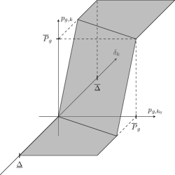
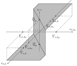
Figure 1: Feasible sets of coupling constraints. (a) corresponds to the feasible set $\mathcal{C}^{p}_{g,k}$ of constraints (10) – (12) in the space of $p_{g,k_{0}}$, $\delta_{k}$, and $p_{g,k}$. (b) corresponds to the feasible set $\mathcal{C}^{v}_{n,g,k}$ of constraints (13) – (15) in the space of $v_{n,k_{0}}$, $v_{n,k}$, and $q_{g,k}$, plotted with the origin at $(v_{n,k_{0}}=1,v_{n,k}=1,q_{g,k}=0)$ for clarity.

Finally, we opted for relaxing complementarity relations in constraints (11), (12), (14) and (15) by replacing $0\leq x\perp y\geq 0$ by $x\geq 0$, $y\geq 0$, and $x\cdot y\leq\epsilon\cdot(\overline{X}-\underline{X})\cdot(\overline{Y}-\underline{Y})$, where $\epsilon$ is a small constant (e.g., $\epsilon=10^{-4}$) and $\underline{X},\overline{X}$ and $\underline{Y},\overline{Y}$ are bounds for $x$ and $y$. This approach can be thought as the middle ground between ill-conditioned smooth equivalents and well-conditioned but loose convex approximations. The non-convex relaxation keeps numerical issues under control (in the worst case, one can simply increase $\epsilon$), while providing almost-feasible solutions, suitable for approximate evaluations within our iterative decomposition procedure for SCACOPF.

Regarding simplifications applied to the formulation of SCACOPF, we note that piecewise linear penalty functions $\gamma^{S},\gamma^{P}$, and $\gamma^{Q}$, nonetheless simple from a theoretical perspective, have a detrimental performance impact, which is due to two main factors. First, these terms are abundant (they are required multiple times for every bus and branch in the power grid) and each of them requires an auxiliary variable and handful of linear constraints to be expressed in a smooth fashion, significantly enlarging the size of the problem to what it would be its size otherwise (approximately by 30%). Secondly, the large slopes of these penalty functions towards large slacks (5 orders of magnitude larger than other terms in the gradient of the objective function and the Jacobian of the constraints (Grid Optimization Competition 2019)) can cause numerical issues whenever they are active (have a positive value). Following these observations, we replaced these penalties functions by quadratic approximations of the form $\tilde{\gamma}(x)=a_{1}x+a_{2}x^{2}$, where $a_{1}$ and $a_{2}$ are computed so as to match the slope of the $\gamma$ functions at the origin and at the beginning of their second bin (corresponding to small slacks). These approximations can be placed directly in the objective avoiding extra variables and constraints. At the same time, our selection of their coefficients prevents the aforementioned numerical issues, without degradation of solution quality in our computational experiments.

4 Decomposition approach

We design our decomposition approach to SCACOPF with the computational and time limitations present in real power grid operations, which were emulated in the GO Competition – Challenge 1: up to 144 parallel processors and either 10 minutes (near-real-time operations) or 45 minutes (offline) maximum elapsed time. Under these restrictions, we can only afford to evaluate contingencies (in parallel) a couple of times (less than 10 for most realistic systems) in order to derive preventive actions in the base case to ensure security constraints are met. These limiting factors on the number of iterations we can perform, along with the non-convexity of subproblems, drove us away from traditional decomposition approaches such as (generalized) Benders and ADMM methods, which typically require tens of iterations to arrive at a good solution. Instead, we develop a specialized approach that derives preventive actions to meet security constraints based on computationally affordable approximations for contingency penalty terms (third and fourth lines in the objective function (16)). We emphasize that our approach is designed to provide good feasible solutions, which do not necessarily satisfy accurately the (local) optimality conditions for problem (1) – (16). Solutions produced by our approach can later be compared against convex relaxations of (1) – (16) (e.g., second-order cone relaxation of base case only) if a quality guarantee is required.

This section presents our decomposition approach for SCACOPF in terms of the subproblems involved, feasibility recovery for contingencies, update rules and our contingency pre-screening methodology, which will become the building blocks for our SCACOPF solver. The particular assembly of these blocks in the asynchronous parallel computing implementation of our SCACOPF solver is discussed later in section 5.

4.1 Subproblems’ formulation

We decompose (1) – (16) – with the approximations described in the preceding section – by stages, leading to a first-stage master subproblem, corresponding to the base case plus penalties coming from the contingencies, and many second-stage subproblems, corresponding to contingencies. We formulate the first-stage master subproblem as

$$\min_{p,q,v,\theta,\sigma}{}{} \sum_{g\in\mathcal{G}^{k_{0}}}f_{g}(p_{g,k_{0}})+\sum_{e\in\mathcal{E}^{k_{0}}}\left(\tilde{\gamma}^{S}(\sigma_{e,o,k_{0}})+\tilde{\gamma}^{S}(\sigma_{e,o,k_{0}})\right)+$$ (18)

$$\sum_{n\in\mathcal{N}}\left(\tilde{\gamma}^{P}(\sigma^{P+}_{n,k_{0}})+\tilde{\gamma}^{P}(\sigma^{P-}_{n,k_{0}})+\tilde{\gamma}^{Q}(\sigma^{Q+}_{n,k_{0}})+\tilde{\gamma}^{Q}(\sigma^{Q-}_{n,k_{0}})\right)+$$

$$\frac{1}{|\mathcal{K}|-1}~{}\sum_{k\in\mathcal{K}\setminus\{k_{0}\}}r_{k}(\boldsymbol{p}_{k_{0}},\boldsymbol{v}_{k_{0}})$$

s.t. $$\eqref{eq:voltage_bounds}\,\text{--}\,\eqref{eq:balance_slacks_nn}:k=k_{0}.$$

where $r_{k}$ are recourse functions corresponding to the objective contributions of second-stage subproblems, i.e., penalties for not abiding with security constraints. Furthermore, the second-stage contingency subproblems that define the functions $r_{k}$ are formulated as

$$r_{j}(\boldsymbol{p}_{k_{0}},\boldsymbol{v}_{k_{0}})=$$ (19)

$$\min_{\begin{subarray}{c}p,q,v,\theta\\ \sigma,\nu,\rho\end{subarray}}{}{} \sum_{e\in\mathcal{E}^{j}}\left(\tilde{\gamma}^{S}(\sigma_{e,o,j})+\tilde{\gamma}^{S}(\sigma_{e,o,j})\right)+$$

$$\sum_{n\in\mathcal{N}}\left(\tilde{\gamma}^{P}(\sigma^{P+}_{n,j})+\tilde{\gamma}^{P}(\sigma^{P-}_{n,j})+\tilde{\gamma}^{Q}(\sigma^{Q+}_{n,j})+\tilde{\gamma}^{Q}(\sigma^{Q-}_{n,j})\right)$$

s.t. $$\eqref{eq:voltage_bounds}\,\text{--}\,\eqref{eq:balance_slacks_nn},\eqref{eq:drop_control},\eqref{eq:v_regulator_diff}:k=j,$$

$$0\leq\rho^{+}_{g,j},\,\rho^{+}_{g,j}\cdot(\overline{P}_{g}-p_{g,j})\leq\epsilon\cdot A_{g}\overline{\Delta}\cdot(\overline{P}_{g}-\underline{P}_{g})~{}~{}\forall g\in\mathcal{G}^{j},$$

$$0\leq\rho^{-}_{g,j},\,\rho^{-}_{g,j}\cdot(p_{g,j}-\underline{P}_{g})\leq\epsilon\cdot-A_{g}\underline{\Delta}\cdot(\overline{P}_{g}-\underline{P}_{g})~{}~{}\forall g\in\mathcal{G}^{j},$$

$$0\leq\nu^{-}_{j,k},\,\nu^{-}_{j,k}\cdot(\overline{Q}_{g}-q_{g,j})\leq\epsilon\cdot(\overline{V}_{n,j}-\underline{V}_{n,k_{0}})\cdot(\overline{Q}_{g}-\underline{Q}_{g})~{}~{}\forall g\in\mathcal{G}^{j}(n),n\in\mathcal{N}^{j},$$

$$0\leq\nu^{+}_{j,k},\,\nu^{+}_{j,k}\cdot(q_{g,j}-\underline{Q}_{g})\leq\epsilon\cdot(\overline{V}_{n,k_{0}}-\underline{V}_{n,j})\cdot(\overline{Q}_{g}-\underline{Q}_{g})~{}~{}\forall g\in\mathcal{G}^{j}(n),n\in\mathcal{N}^{j},$$

for all $j\in\mathcal{K}\setminus\{k_{0}\}$.

We observe that the master subproblem (18) and the contingency subproblems (19) share the main OPF structure but are different in two key aspects: (i) subproblem (19) does not take production cost into consideration, and (ii) subproblem (19) is further restricted by the (approximate) drop frequency control and voltage regulator constraints. Despite these additional constraints subproblem (19) will be feasible as long as $(\boldsymbol{p}_{k_{0}},\boldsymbol{v}_{k_{0}})$ is feasible for (18) to construct a feasible solution it suffices to take $\boldsymbol{p}_{j}=\boldsymbol{p}_{k_{0}}$ and $\boldsymbol{v}_{j}=\boldsymbol{v}_{k_{0}}$, and compute values for the remaining variables accordingly. Such solution would be feasible even for $\epsilon=0$, satisfying constraints (10) – (15) exactly, nevertheless this solution tends to be bad due to significant activation of power balance slacks which result in large penalties. The next subsection examines how to recover good feasible solutions for contingency subproblems (19) satisfying constraints (10) – (15) exactly.

4.2 Feasibility recovery for contingency subproblems

There are two situations under which we may require a fully feasible contingency solution: (i) a system operator would like to study how the system would respond to a certain contingency or (ii) we need a better estimate for the contingency penalties because the relaxation (19) is lose, and further decreasing $\epsilon$ is time consuming and prone to numerical issues. We handle these situations by, first, solving the relaxed contingency subproblem (19) with $\epsilon>0$ and then crushing the approximate solution onto the exact feasible set according to the procedure outlined below.

Let $(\boldsymbol{\tilde{p}}_{j},\boldsymbol{\tilde{q}}_{j})$ be an solution to problem (19) with $\epsilon>0$ for certain $j\in\mathcal{K}\setminus\{k_{0}\}$, and let

$$\min_{\begin{subarray}{c}p,q,v,\theta\\ \sigma,\nu,\rho\end{subarray}}{}{} \sum_{e\in\mathcal{E}^{j}}\left(\tilde{\gamma}^{S}(\sigma_{e,o,j})+\tilde{\gamma}^{S}(\sigma_{e,o,j})\right)+$$ (20)

$$\sum_{n\in\mathcal{N}}\left(\tilde{\gamma}^{P}(\sigma^{P+}_{n,j})+\tilde{\gamma}^{P}(\sigma^{P-}_{n,j})+\tilde{\gamma}^{Q}(\sigma^{Q+}_{n,j})+\tilde{\gamma}^{Q}(\sigma^{Q-}_{n,j})\right)$$

s.t. $$\eqref{eq:voltage_bounds}\,\text{--}\,\eqref{eq:balance_slacks_nn}:k=j$$

be a canvas for the restricted contingency subproblem, which will be modified during the crushing procedure. Additionally, let’s define the function $\Delta_{j}:\Omega\rightarrow\mathbb{R}$ where $\Omega=\big{\{}(x,\boldsymbol{p}_{k_{0}})\in\mathbb{R}\times[\boldsymbol{\underline{P}},\boldsymbol{\overline{P}}]\big{|}\sum_{g\in\mathcal{G}^{j}:A_{g}>0}(\underline{P}_{g}-p_{g,k_{0}})<x<\sum_{g\in\mathcal{G}^{j}:A_{g}>0}(\overline{P}_{g}-p_{g,k_{0}})\big{\}}$ as

$$\Delta_{j}\left(x,\boldsymbol{p}_{k_{0}}\right):={} \Bigg{\{}\delta_{j}\in\mathbb{R}~{}\Big{|}~{}\exists(\boldsymbol{p}_{j},\boldsymbol{\rho}^{+}_{j},\boldsymbol{\rho}^{-}_{j})\in\mathbb{R}^{3|\mathcal{G}^{j}|}~{}\text{s.t.}~{}$$

$$\eqref{eq:drop_control}\text{--}\eqref{eq:drop_control_down_saturation}:k=j,~{}\sum_{g\in\mathcal{G}^{j}:A_{g}>0}(p_{g,j}-p_{g,k_{0}})=x\Bigg{\}}.$$

In words, $\Delta_{j}$ returns the value of $\delta_{j}$ that would cause an increase/decrease of production $x$ in contingency $j$ with respect to a base case production set point $\boldsymbol{p}_{k_{0}}$. In practice, this function can be implemented with a for loop over the generators in $\mathcal{G}^{j}$, performing a line search over $\delta_{k}$ ($x$ can be computed in a straightforward fashion from $\delta_{k}$ and $\boldsymbol{p}_{k_{0}}$).

Then, we proceed as follows. We formulate the restricted (canvas) contingency subproblem (20). In order to satisfy the frequency drop constraints, (10) – (12), we modify the restricted subproblem as indicated Alg. 1. In the same fashion, in order to satisfy the voltage regulation constraints, (13) – (15), we further modify the restricted subproblem following Alg. 2. Finally, we solve the modified restricted contingency subproblem to obtain a solution satisfying all contingency $j$’s constraints in the original SCACOPF problem. This procedure can be repeated for all contingencies to generate a complete feasible solution to SCACOPF.

Input: base case solution $\boldsymbol{p}_{k_{0}}$, approximate contingency solution $\boldsymbol{\tilde{p}}_{j}$.

compute $\hat{\delta}_{j}:=\Delta_{j}\big{(}\sum_{g\in\mathcal{G}^{j}}\tilde{p}_{g,j},\boldsymbol{p}_{k_{0}}\big{)}$;

compute $\hat{p}_{g}:=\max\{\min\{p_{g,k_{0}}+A_{g}\hat{\delta}_{j},\overline{P}_{g}\},\underline{P}_{g}\}$ for all $g\in\mathcal{G}^{j}$ ;

if $\hat{\delta}_{j}\geq 0$ then

       let $\check{\mathcal{G}}=\{g\in\mathcal{G}^{j}|\hat{p}_{g}=\overline{P}\}$ and compute $\underline{D}=\max_{g\in\check{\mathcal{G}}}(\overline{P}_{g}-p_{g,k_{0}})/A_{g}$ ;

       let $\hat{\mathcal{G}}=\{g\in\mathcal{G}^{j}|\hat{p}_{g}<\overline{P}\}$ and compute $\overline{D}=\min_{g\in\hat{\mathcal{G}}}(\overline{P}_{g}-p_{g,k_{0}})/A_{g}$ ;

       with problem (20) do

             fix $p_{g,j}=\overline{P}_{g}$ for all $g\in\check{\mathcal{G}}$ ;

             set bounds $\underline{D}\leq\delta_{j}\leq\overline{D}$ ;

             add constraints $p_{g,j}=p_{g,k_{0}}+A_{g}\delta_{j}~{}~{}\forall g\in\hat{G}$ ;

            

       end

      

else

       let $\check{\mathcal{G}}=\{g\in\mathcal{G}^{j}|\hat{p}_{g}>\underline{P}\}$ and compute $\underline{D}=\max_{g\in\check{\mathcal{G}}}(\underline{P}_{g}-p_{g,k_{0}})/A_{g}$ ;

       let $\hat{\mathcal{G}}=\{g\in\mathcal{G}^{j}|\hat{p}_{g}=\underline{P}\}$ and compute $\overline{D}=\min_{g\in\hat{\mathcal{G}}}(\underline{P}_{g}-p_{g,k_{0}})/A_{g}$ ;

       with problem (20) do

             fix $p_{g,j}=\overline{P}_{g}$ for all $g\in\hat{\mathcal{G}}$ ;

             set bounds $\underline{D}\leq\delta_{j}\leq\overline{D}$ ;

             add constraints $p_{g,j}=p_{g,k_{0}}+A_{g}\delta_{j}~{}~{}\forall g\in\check{G}$ ;

            

       end

      

end if

Algorithm 1 Crushing procedure for frequency drop control constraints (10) – (12).

Input: base case solution $\boldsymbol{v}_{k_{0}}$, approximate contingency solution $\boldsymbol{\tilde{q}}_{j}$, tolerance $\epsilon^{q}$.

for $n\in\mathcal{N}^{j}$ do

       compute $\hat{\eta}=\big{(}\sum_{g\in\mathcal{G}^{j}(n)}\tilde{g}_{g,j}\big{)}/\big{(}\sum_{g\in\mathcal{G}^{j}(n)}(\overline{Q}_{g}-\underline{Q}_{g})\big{)}$ ;

       with problem (20) do

             if $\hat{\eta}<\epsilon^{q}$ then

                   fix $q_{g,j}=\underline{Q}_{g}$ for all $g\in\mathcal{G}^{j}(n)$ ;

                   set bounds $v_{n,k_{0}}\leq v_{n,j}\leq\overline{V}_{n,j}$ ;

                  

             else if $\epsilon^{q}\leq\hat{\eta}\leq 1-\epsilon^{q}$ then

                   fix $v_{n,j}=v_{n,k_{0}}$ ;

                  

             else

                   fix $q_{g,j}=\overline{Q}_{g}$ for all $g\in\mathcal{G}^{j}(n)$ ;

                   set bounds $\overline{V}_{n,j}\leq v_{n,j}\leq v_{n,k_{0}}$ ;

                  

             end if

            

       end

      

end for

Algorithm 2 Crushing procedure for voltage regulators’ constraints (13) – (15).

4.3 Recourse functions approximation and surrogate block-incremental algorithm

The key idea of our approach for handling contingencies is to approximate the recourse functions $r_{k}$ in the base case subproblem (18) via low-dimensional surrogates that can be, both, handled easily by nonlinear programming solvers and updated easily after a subset of the contingencies is evaluated. Specifically, for generator contingencies $\mathcal{K}^{\mathcal{G}}\subset\mathcal{K}$ we propose the surrogate

$$\tilde{r}_{k}\left(p_{g(k),k_{0}},q_{g(k),k_{0}}\right)=P_{k}\cdot\left(p_{g(k),k_{0}}^{2}+q_{g(k),k_{0}}^{2}\right)^{2}$$

where $g(k)=\mathcal{G}^{k_{0}}\setminus\mathcal{G}^{k}$, that is, $g(k)$ is the failing generator in contingency $k\in\mathcal{K}^{\mathcal{G}}$ and $P_{k}\geq 0$ is a constant to be determined. This surrogate was inspired by three observations. First, the economics of SCACOPF (generation cost) drive the solution towards a very limited subset of the feasible space (essentially, following merit order) where most generators that are producing do so at their upper capacity limit. Second, within this subset, penalties for contingencies tend to decrease whenever the quantity injected by the failing generator is decreased (in the limit, if the generator injects zero MVA to the network, the contingency has no effect whatsoever on the network). Third, the penalty decrease with the injection is typically very steep and local. Trying to emulate the phenomena in the prior observations, the proposed surrogate penalizes the fourth power of the apparent power of the failing generator, pushing the base case towards a more risk averse solution with a rapidly increasing penalty. We compute $P_{k}$ from one evaluation of $r_{k}(\boldsymbol{p}_{k_{0}},\boldsymbol{v}_{k_{0}})$ as $P_{k}:=r_{k}\big{(}\boldsymbol{p}_{k_{0}},\boldsymbol{v}_{k_{0}}\big{)}/\big{(}p_{g(k),k_{0}}^{2}+q_{g(k),k_{0}}^{2}\big{)}^{2}$, so that $\tilde{r}_{k}\big{(}p_{g(k),k_{0}},q_{g(k),k_{0}}\big{)}=r_{k}\big{(}\boldsymbol{p}_{k_{0}},\boldsymbol{v}_{k_{0}}\big{)}$ and $\tilde{r}_{k}\big{(}0,0\big{)}=0$.

We follow the same reasoning for branches (power lines and transformers) and penalize the apparent power entering the failing branch at the terminal where it is the highest, for all branch contingencies $k\in\mathcal{K}^{\mathcal{E}}$. These surrogates produce good feasible solutions to the SCACOPF problem (1) – (16) using Alg. 3 followed by a round of feasibility recovery to obtain contingency solutions.

Input: maximum number of iterations $T$, recourse penalty tolerance $\epsilon^{r}$

set $P_{k}:=0$ for all $k\in\mathcal{k}\setminus\{k_{0}\}$ ;

for $t=1:T$ do

       solve base case subproblem (18) with surrogate recourse ;

       select a block of contingencies $\mathcal{K}^{t}\subseteq(\mathcal{K}\setminus\{k_{0}\})$ ;

       solve contingency subproblem (19) for all $k\in\mathcal{K}^{t}$ ;

       update $P_{k}:=r_{k}\big{(}\boldsymbol{p}_{k_{0}},\boldsymbol{v}_{k_{0}}\big{)}/\big{(}p_{g(k),k_{0}}^{2}+q_{g(k),k_{0}}^{2}\big{)}^{2}$ for all $k\in\mathcal{K}^{t}\cap\mathcal{K}^{\mathcal{G}}$ ;

       update $P_{k}:=r_{k}\big{(}\boldsymbol{p}_{k_{0}},\boldsymbol{v}_{k_{0}}\big{)}/\big{(}p_{e(k),i,k_{0}}^{2}+q_{e(k),i,k_{0}}^{2}\big{)}^{2}$ for all $k\in\mathcal{K}^{t}\cap\mathcal{K}^{\mathcal{E}}$, where $i=\argmax_{j\in\{o(e),d(e)\}}p_{e(k),j,k_{0}}^{2}+q_{e(k),j,k_{0}}^{2}$ ;

       if (19) evaluated & $r_{k}\big{(}\boldsymbol{p}_{k_{0}},\boldsymbol{v}_{k_{0}}\big{)}<\epsilon^{r}$ for all $k\in\mathcal{K}^{t}$ then

            break ;

       end if

      

end for

return current base case solution ;

Algorithm 3 Surrogate block-incremental algorithm for SCACOPF.

Algorithm 3 is easily parallelizable (evaluation of contingency subproblems), it allows for (almost) arbitrary selection of blocks of contingencies to evaluate at each iteration, and it allows for asynchronous updates, that is, in a parallel computing setting we can solve the base case continuously and update the surrogates as new contingency evaluations are completed. On the selection of contingency blocks, reasonably, we would like to start evaluating contingencies that are likely to have a large impact on the problem. How to find these contingencies quickly and limit their impact early on is the topic of the next subsection.

4.4 Contingency pre-screening

Our initial approach to ranking contingencies and selecting a subset of likely impactful contingencies was based on machine learning methodologies. This approach, whereas promising in general, failed to provide a good ranking or classification of contingencies, its main problem being the difficulty of generalizing machine learning models to networks that have not been seen before in the training datasets (Yang and Oren 2019). Other methodologies from the literature required extensive calculations, which were not practical for near-real-time settings (Capitanescu et al. 2007, Fliscounakis et al. 2013). Instead, we use intuitive selection rules, cheap to compute and with good generalization: we select the $S^{\mathcal{G}}$ largest generator failures and $S^{\mathcal{E}}$ largest branch failures (in terms of the elements’ capacities), with $S^{\mathcal{G}}+S^{\mathcal{E}}$ smaller or equal to the number of parallel processors available for contingency evaluations. This procedure tends to produce some false positives (contingencies that look impactful but are not) but almost no false negative (contingencies that look harmless but are impactful), both situations easily remediable by exploiting parallel computing.

5 Computational and implementation aspects

We designed our software framework, gollnlp, with software re-usability in mind. To this end, we developed a lightweight model specification library that allows a modular composition of the various algebraic ACOPF and SCACOPF models instantiated by our solution approach. These developments and underlying high-performance computing aspects are discussed in detail in Section 5.1. Furthermore, the gollnlp framework has a solver-agnostic back-end that allows switching between different NLP solvers. At the moment we support Ipopt (Wätcher and Biegler 2006) and HiOp (Petra 2019). We performed a couple of customizations specific to Ipopt for the purpose of improving robustness and reduce computational cost. These are further elaborated in Section 5.3.

In order to obtain a good computational parallelization efficiency of the decomposition approach presented in Section 4, we implemented a nonblocking/asynchronous parallel evaluation engine for performing the computational analysis of the contingency subproblems and for building their recourse evaluations presented in Sections 4.1–4.3. The implementation is based on the Message Passing Interface (MPI) and is presented in Section 5.2

5.1 Model evaluation library

The specification of SCACOPF problem (1) – (16) is done via lightweight C++ library that evaluates the objective and constraints functions, and their first and second order derivatives, as required by the underlying NLP solvers. Both the functions and their derivatives defining the problem (1) – (16) are “hand-coded” in C++. The specification library is modular in the sense it can assemble and manipulate generic NLPs such as ACOPF, as well instantiate the NLPs in the low level format of supported NLP solvers, from existing objective and constraint C++ classes. The objective can be formed by an arbitrary number of additive objective terms, such as generation cost, penalties, various recourse approximations, primal regularization terms, etc. The constraints of the NLP is simply a list of (sparse) constraints of blocks of constraints. The library supports instantiating SCACOPF problems containing a base case ACOPF block and multiple contingencies blocks and is aware of the underlying problem structure; however, our computational methodology does not use this feature since our optimization-based decomposition approach instantiates the first-stage master and second-stage contingency blocks as separate problems (with the contingency subproblem being parameterized by the first-stage’s coupling variables).

Ipopt and HiOp NLP solvers require function values and gradient values as double arrays. The Jacobian of the constraints and the Hessian of the Lagragian are evaluated as sparse matrices in triplet format. The assembly and repeated evaluation of the sparse derivatives throughout the NLP solver iterations may easily take a high computational cost because of the high cost associated with (random) lookups (i.e., locating and accessing a given entry) in a sparse matrix. These lookups occur every time when a objective or constraint blocks update the derivative matrix with their (sparse) contribution and have non-trivial complexity (meaning greater than $O(1)$) in general. We circumvent this by adding a one-time preprocessing step that for each objective or constraint block builds an array of pointers to the block’s nonzeros in the sparse derivative. During this preprocessing step, we sort the nonzeros based on their row and column indexes and remove duplicate entries. Consequently, the time complexity of the preprocessing step is $O(\zeta log\zeta)$ and the space requirements are $\zeta$, where $\zeta$ is the sum of the number of nonzeros of each objective or constraint block. On the other hand, we achieve $O(1)$ random access to the nonzero entries of the sparse derivative; this enables derivative evaluation at O($\zeta$) time complexity and amortizes the cost of the preprocessing step over over the course of NLP solver iterations. As a result, the evaluation of NLP consistently requires a very small fraction ($<1\%$) of the total computational cost.

5.2 Parallel computations

As mentioned in Section 4, the contingency subproblems (19) can be solved independently, in parallel, for a given solution of the master subproblem (18). The obvious parallelization approach, usually known as master–worker parallelization, is to dedicate a small subset of the computing units to the first-stage subproblem and the rest to the contingency subproblems. Each time all the contingencies are evaluated, the workers send the recourse approximations to the master unit, which in turn resolves the first-stage problem and dispatches the solution to the worker units, effectively starting a new iteration of the algorithm.

This above simple parallel programming model suffers from a couple important drawbacks. Computational load imbalance is significant, being caused by the considerable variation across the wall-clock (solution) times for the contingency subproblems in the worker units. This is especially pervasive when end-of-iteration synchronization between master and worker units is enforced. An extreme, but quite frequent, consequence of this limitation manifests in a considerable number of worker computing units sit idle for extended amount of time waiting for a couple tardy workers to finish contingency evaluations. The second limitation of a simple master–worker model would be caused by the fact that all worker units sit idle while the master unit solves the first-stage subproblem. Finally, the master unit(s) performs significant bookkeeping, file operations, and communication with the workers; as a result, the master unit may use only a subset of its compute cycles to solve the first-stage subproblem. We remark that this results in a domino effect, as it will delay not only the first-stage solution but will also keep all the workers idle for longer.

We address the above limitations by using a more involved master–solver–worker parallel programming model, in which, one of the compute units is solely assigned to solving the first-stage subproblem (hence the name solver). This allows the master unit to be dedicated to algorithm control loops, file input/out, and communication. We employ a distributed memory programming model that results in the master, solver, and workers units to run in independent processes; MPI is used for (inter-process) communication. Furthermore, the communication uses only nonblocking MPI calls, more specifically, only MPI_Isend and MPI_Irecv. While this choice complicates the implementation significantly because the completion of each message needs to be checked periodically, it has the important benefit of overlapping communication with computations. This is especially relevant to master, which otherwise will be unable to timely handle the algorithm control loops and the communication in the same time.

The worker and the solver units engage in communication only with the master. The master decides the apportionment of contingencies subproblems to worker processes and schedules only one contingency at a time per worker process, which is paramount to ensure good load balancing across the workers. The contingency subproblems are initially prioritized based on the rankings found in the pre-screening of Section 4.4; later on, the contingencies found to have high penalties are rescheduled for reevaluation/re-approximation. The master–worker conversation comprises of predefined basic actions: (i) master asks worker to evaluate a contingency, (ii) worker provides contingency recourse approximation to the master, and (iii) initialization and finalization. On the other hand, the master–solver conversation is quite simple and it involves only solve “start” and “completion” actions. In general, the master instructs the solver process to reevaluate first-stage subproblem once it receives a few high-penalty contingency recourse approximations from the workers. We remark that the solver process solves the base case problem without forcing the master or worker processes to sit idle; instead, these processes can continue evaluating and approximating contingencies. Under a strict computational budget, this approach can increase the number of evaluated contingencies by more than $250\%$ over plain master–worker parallelization paradigms. The downside of our approach is that the master subproblem is updated with recourse approximations asynchronously and possibly is using outdated recourse approximations built around first-stage set points from previous iterations. The convergence of such asynchronous solver–worker scheme is problematic, especially for non-convex problems such as SCACOPF. The use of recourse surrogates based on the fourth power of the apparent power (instead of using similar quadratic surrogates) has shown a considerable stabilization effect on the convergence the asynchronous algorithm in our extensive numerical experiments. We believe that this is likely caused by the fact that the steep fourth order surrogates serve as an effective proximal point term on the first-stage variables. Future work will be dedicated to further investigate and develop globally convergent variants of this asynchronous solver–worker method.

5.3 Other implementation details

Since a great reduction of computational cost is obtained from warm-starting, we elaborate on our experience with warm-starting interior-point methods when resolving the first-stage and the contingency subproblems. In our computational scheme, the first-stage subproblem can be warm-started efficiently, for $50-80\%$ reduction in the computational cost, by reusing the primal-dual solution occurring during the previous first-stage solve for a log barrier parameter around $10^{-5}$. For the contingency subproblems, the best overall performance is obtained when only a primal restart is done using the solution from the first-stage problem. For these subproblems primal-dual restarts tends to give less benefits, regardless of using solutions from the previously solved contingency subproblem or from the first-stage subproblem. This is mainly because a nontrivial number of contingencies converge very slowly when using primal-dual restarts. To some extent, this also applies when solving the feasibility recovery subproblems, described in Section 4.2.

Given the large size and the considerable number of contingencies of the SCACOPF problem solved, the number of NLP subproblems that needs to be solved can be as high as 100 000, each of 2 000 0000 variables and constraints. In this large-scale computational regime, the possibility of unexpected software failures cannot be dismissed. Surprisingly, we experienced only a couple of nontrivial issues because Ipopt is extremely robust. A repeated issue, among these, was an occasional solver divergence or convergence to a locally infeasible point when solving the contingency subproblems. The issue tends to occur when solving the feasibility recovery contingency subproblems. We could not find a sound explanation for it since the problems are provably feasible and we alleviate these issues by adding small quadratic regularization terms in the objective for the voltages and angles. By far the most troubling issue we ran into was that MPI worker processes occasionally seemed to hang and – on rare occasions – to crash with SIGBUS or SIGSEGV signals, depending on the platform and/or compilers. This issue is aggravated because a crash in one MPI process would cause all the MPI processes to stop execution as per the MPI standard. The apparent source of the hang or crash was the combination of Ipopt and the HSL MA57 linear solver, but we could not find the cause of the abnormal runtime behavior. We addressed this with a three-pronged approach. First we modified Ipopt to throw an exception when the linear solver unexpectedly requires a large memory reallocation; we handled this instructing Ipopt to switching to MA27 linear solver and resolve the problem. The second freeze and/or crash mitigation approach was to set an alarm (a.k.a. a timeout SIGALRM signal) before each call to the MA57 faulty function and whenever the alarm signal was generated (meaning that MA57 faulty function takes an unexpectedly long time), we modified Ipopt to throw an exception; in which case, gollnlp instructs Ipopt to use MA27 on resolve. Interceptions of signals associated with the runtime crash were also implemented as last resort, to prevent MPI processes from failing.

6 Numerical results

During the course of Challenge 1, the performance of gollnlp was evaluated independently by the organizers of the GO competition using synthetic and real SCACOPF instances. In this section we focus on two aspects of the results of those experiments. First, we explore the qualitative differences between an ACOPF solution and the SCACOPF solution found by our method, for a realistic synthetic instance, and explain how such SCACOPF solution is achieved. Second, we provide a summary of the comparative performance of gollnlp in the Final Event of Challenge 1.

6.1 ACOPF vs gollnlp’s SCACOPF solution

We compare two approaches for scheduling power system operations: (i) ACOPF, that is, we solve the plain ACOPF problem and then evaluate its performance including contingencies, and (ii) SCACOPF, e.g., solving SCACOPF using gollnlp. For this comparison, we use the synthetic version of the Western Electricity Coordinating Council (WECC) developed by Birchfield et al. (2017), which we augmented with frequency drop control parameterd derived from Challenge 1 instances, stricter branch capacities based on simulations over 12 representative load cases, and randomly generated contingencies. The resulting instance has 10 000 buses, 12 707 branches, 2 485 generators, 10 000 contingencies, and 4 899 consumers totalling 133.1 GW of load.

Figure 2 presents a depiction of the base case solution of ACOPF (a) and the difference on the base case solutions between SCACOPF and ACOPF (b). ACOPF schedules production minimizing base case operating cost only, thereby, setting the cheapest generator to operate at their capacity, which tends to concentrate power generation. SCACOPF, in contrasts, spreads out production – as can be seen in Fig. 2(b) – in order to hedge against failures. gollnlp achieves this hedging strategy starting from the ACOPF solution and progressively adding approximate recourse terms penalizing activity on elements that might fail. The mechanism at work can be appreciated in Fig. 3. The ACOPF solution evaluated for a transformer contingency shows a large imbalance (Fig. 3(b)) because a generator behind the transformer is dispatched at capacity in the base case and cannot reduce its power output post-contingency due to frequency drop control constraints. gollnlp adds a recourse term penalizing the flow over the failing transformer, which in turn rewards a reduction in the base case dispatch of the generator behind the transformer in the SCACOPF solution with respect to ACOPF solution (Fig. 3(a)). As a result of this dispatch reduction, the imbalance in the post-contingency state of SCACOPF decreases significantly (more than 100MW) with respect to that of ACOPF, as can be seen in Fig. 3(c). This example illustrates how our non-convex relaxation of the coupling constraints along with our recourse approximation serve to effectively characterize and hedge against contingencies in SCACOPF.

(a)

(b)

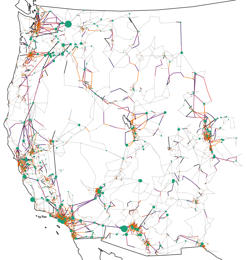
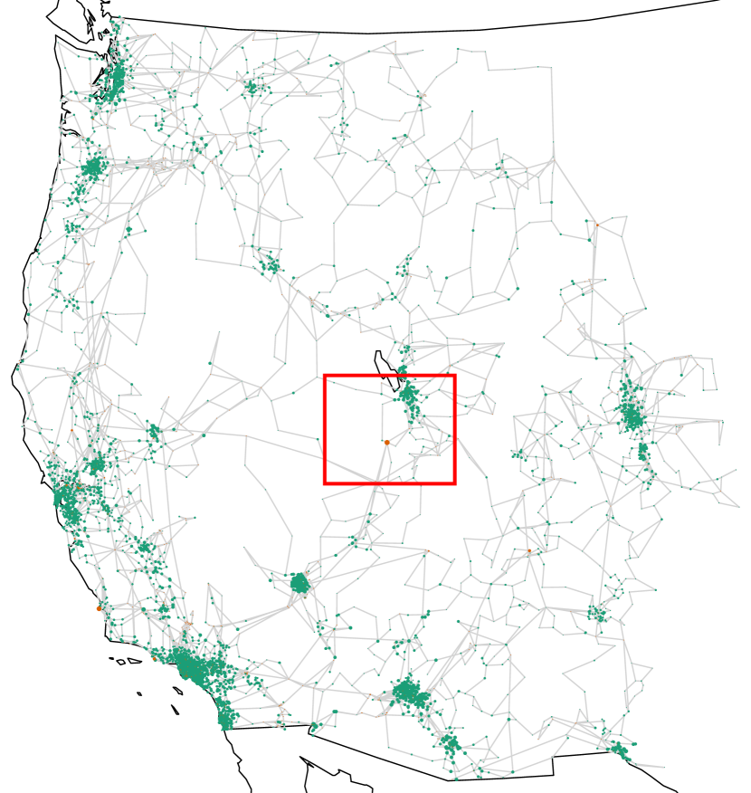
Figure 2: Synthetic WECC network color coded with ACOPF and SCACOPF base case solutions. Part (a) presents the ACOPF base case solution. Vertices correspond to substations, colored green for substations injecting active power (generators) and orange for substations withdrawing active power, with their area being proportional to the injected/withdrawn active power. Edges corresponds to groups of lines between substations. They are colored according to remaining power margin at the solution, the darker the color the smaller the margin to congestion. Part (b) presents the injection/withdraw differences between SCACOPF and ACOPF. For vertices, green indicates an increase in injection, orange indicates a decrease in injection, and the area of each vertex is proportional to the injection difference. No information encoded for edges. The red box delimits an area of interest, depicted in detail in Fig. LABEL:fig:zomm_box_contingency.

(a)

(b)

(c)

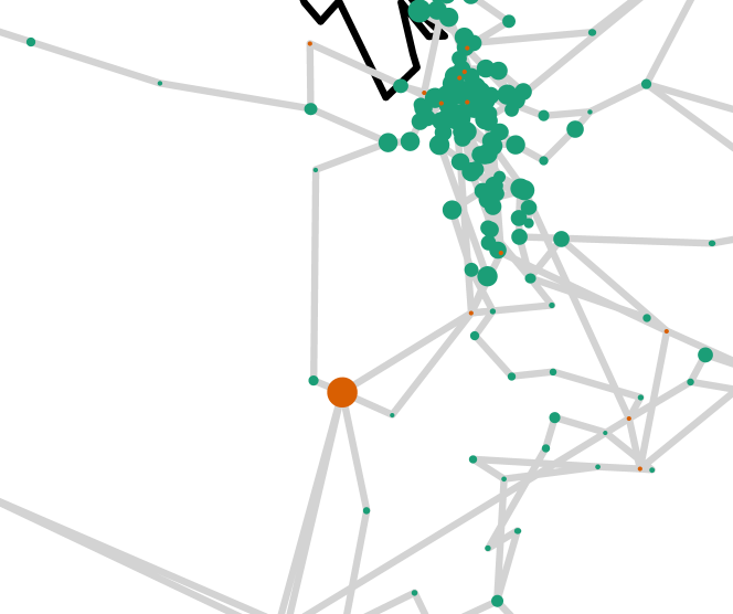
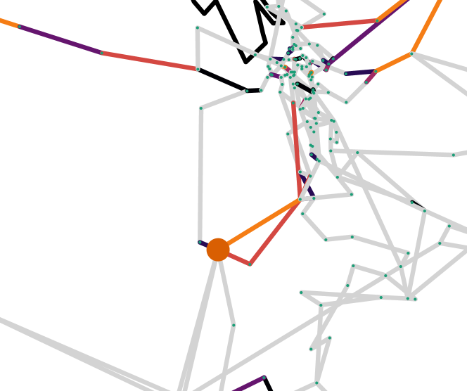
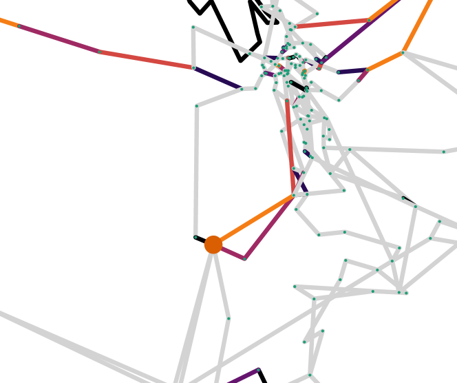
Figure 3: Differences in base case and contingency solution between ACOPF and SCACOPF for synthetic WECC network. Part (a) zooms in to the area delimited with a red box in Fig. 2.(c). Part (b) presents the post-contingency solution of ACOPF for the failure of a transformer at substation “DELTA 2” at the center of the plot. Orange vertices indicate positive active imbalances (production shedding) green vertices indicate negative imbalances (load shedding), with their area being proportional to the imbalance amount. Edges colored as in Fig. 2.(a). Part (c) presents the post-contingency solution of SCACOPF for the same contingency, color coded in the same fashion as (b).

6.2 Benchmarking

Our approach was benchmarked against other competing approaches in the Final Event of Challenge 1 (Grid Optimization Competition 2020), over 17 synthetic network models with 20 scenarios each, 10 scenarios corresponding to Division 1 with a time limit of 10 minutes, and the other 10 scenarios corresponding to Division 2 with a time limit of 45 minutes. All competing approaches ran on the same platform, consisting of 6 nodes equipped with 2 Intel Xeon E5-2670 v3 (24 cores per node) and 64 GB of RAM per node, intended to represent the computational resources currently in use by power system operators. We would like to remark that gollnlp is not bound to these hardware specifications and it has been deployed from personal laptops up to hundred of nodes of high-end supercomputers, such as Summit at Oak Ridge National Laboratory.

Figures 4 and 5 present our aggregate performance for each network in Division 1 and Division 2, respectively, against the best 50% objective values in each division for each network, among those able to obtain feasible solutions. As can be observed, our approach consistently obtained the best or very close to the best known feasible solution across a wide range of system sizes and in both Division 1 and Division 2.

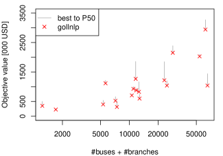
Figure 4: Comparative performance of gollnlp in Division 1 of Challenge 1. Plot presents ranges of geometric mean objective value for every synthetic network tested in the Final Event (lower is better).

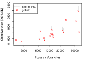
Figure 5: Comparative performance of gollnlp in Division 2 of Challenge 1. Plot presents ranges of geometric mean objective value for every synthetic network tested in the Final Event (lower is better).

7 Conclusions

We have presented a computational approach for obtaining good feasible solutions to the SCACOPF problem at real-world scale and under real-world time limits. Our method relies on state-of-the-art non-linear programming algorithms and it uses non-convex relaxations of complementarity constraints, two-stage decomposition with sparse approximations of recourse terms, and asynchronous parallelism, in order to compute SCACOPF base case solutions that hedge against contingencies. The method was benchmarked independently and found to consistently produce high quality solutions across a wide range of network sizes and difficulty, thereby providing an effective complement to the extensive literature on bounding via convex relaxations.

Future work will investigate the efficient use of emerging computing hardware accelerators (e.g., GPUs) for SCACOPF problems, as well as its global solution using branch-and-bound techniques that integrate convex relaxations and strengthening with the present work.

Endnotes

1. 1 Specifically, we do not present the models for transformer branches and switched shunts, the models for piecewise linear costs and penalty functions, and we do not consider multiple areas when presenting the model for frequency drop control, nor the case where these controllers may have negative constants. The complete model can be found in (Sec. 3 ARPA-E GO Comp. 2019).
2. 2 The Final Event also included 3 industry network models with 4 scenarios each. We do not include statistics on those networks in the paper as detailed results on those networks remain confidential.

8 Acknowledgments

This work performed under the auspices of the U.S. Department of Energy by Lawrence Livermore National Laboratory under Contract DE-AC52-07NA27344.

This document was prepared as an account of work sponsored by an agency of the United States government. Neither the United States government nor Lawrence Livermore National Security, LLC, nor any of their employees makes any warranty, expressed or implied, or assumes any legal liability or responsibility for the accuracy, completeness, or usefulness of any information, apparatus, product, or process disclosed, or represents that its use would not infringe privately owned rights. Reference herein to any specific commercial product, process, or service by trade name, trademark, manufacturer, or otherwise does not necessarily constitute or imply its endorsement, recommendation, or favoring by the United States government or Lawrence Livermore National Security, LLC. The views and opinions of authors expressed herein do not necessarily state or reflect those of the United States government or Lawrence Livermore National Security, LLC, and shall not be used for advertising or product endorsement purposes.

References

- Alsac et al. (1990) Alsac O, Bright J, Prais M, Stott B (1990) Further developments in lp-based optimal power flow. IEEE Transactions on Power Systems 5(3):697–711.
- Alsac and Stott (1974) Alsac O, Stott B (1974) Optimal load flow with steady-state security. IEEE Transactions on Power Apparatus and Systems PAS-93(3):745–751.
- Bai et al. (2008) Bai X, Wei H, Fujisawa K, Wang Y (2008) Semidefinite programming for optimal power flow problems. International Journal of Electrical Power & Energy Systems 30(6):383 – 392, ISSN 0142-0615.
- Birchfield et al. (2017) Birchfield AB, Xu T, Gegner KM, Shetye KS, Overbye TJ (2017) Activsg10k: 10000-bus synthetic grid on footprint of western united states. URL https://electricgrids.engr.tamu.edu/electric-grid-test-cases/activsg10k/, accessed 2021-02-25.
- Bouffard et al. (2005) Bouffard F, Galiana F, Arroyo JM (2005) Economic dispatch with security using nonlinear programming. XV Power Systems Computation Conference, 1–7.
- Boyd and Vandenberghe (2004) Boyd S, Vandenberghe L (2004) Convex Optimization (Cambridge University Press).
- Bruno et al. (2002) Bruno S, De Tuglie E, La Scala M (2002) Transient security dispatch for the concurrent optimization of plural postulated contingencies. IEEE Transactions on Power Systems 17(3):707–714.
- Capitanescu et al. (2007) Capitanescu F, Glavic M, Ernst D, Wehenkel L (2007) Contingency filtering techniques for preventive security-constrained optimal power flow. IEEE Transactions on Power Systems 22(4):1690–1697.
- Capitanescu and Wehenkel (2011) Capitanescu F, Wehenkel L (2011) Redispatching active and reactive powers using a limited number of control actions. IEEE Transactions on Power Systems 26(3):1221–1230.
- Carpentier (1962) Carpentier J (1962) Contribution a l’etude du dispatching économic. Bulletin de la Societé Française des Électriciens, 431 – 434, number vol. III in 8.
- Carpentier (1979a) Carpentier J (1979a) Optimal power flows. International Journal of Electrical Power & Energy Systems 1(1):3 – 15, ISSN 0142-0615.
- Carpentier (1979b) Carpentier J (1979b) Optimal voltage scheduling and control in large power systems. IFAC Proceedings Volumes 12(5, Part 2):210 – 216, ISSN 1474-6670, symposium on Computer Applications in Large Scale Power Systems Volume 2, New Dehli, India, 16-19 August.
- Chen et al. (2008) Chen JS, Sun D, Sun J (2008) The sc1 property of the squared norm of the soc fischer–burmeister function. Operations Research Letters 36(3):385 – 392.
- Cory and Henser (1972) Cory B, Henser P (1972) Economic dispatch with security using nonlinear programming. IV Power Systems Computation Conference, 1–12.
- Dvorkin et al. (2018) Dvorkin Y, Henneaux P, Kirschen DS, Pandžić H (2018) Optimizing primary response in preventive security-constrained optimal power flow. IEEE Systems Journal 12(1):414–423.
- Ekisheva and Gugel (2015) Ekisheva S, Gugel H (2015) North American AC circuit outage rates and durations in assessment of transmission system reliability and availability. 2015 IEEE Power Energy Society General Meeting, 1–5.
- Elacqua and Corey (1982) Elacqua AJ, Corey SL (1982) Security constrained dispatch at the new york power pool. IEEE Transactions on Power Apparatus and Systems PAS-101(8):2876–2884.
- Fliscounakis et al. (2013) Fliscounakis S, Panciatici P, Capitanescu F, Wehenkel L (2013) Contingency ranking with respect to overloads in very large power systems taking into account uncertainty, preventive, and corrective actions. IEEE Transactions on Power Systems 28(4):4909–4917.
- Grid Optimization Competition (2019) Grid Optimization Competition (2019) Scopf problem formulation: Challenge 1. Available at: https://gocompetition.energy.gov/challenges/challenge-1/formulation.
- Grid Optimization Competition (2020) Grid Optimization Competition (2020) Leaderboard - challenge 1 - final event. Available at: https://gocompetition.energy.gov/challenges/challenge-1/leaderboards-final-event.
- Jabr (2006) Jabr RA (2006) Radial distribution load flow using conic programming. IEEE Transactions on Power Systems 21(3):1458–1459.
- Karoui et al. (2008) Karoui K, Crisciu H, Stubbe M, Szekut A (2008) Large scale security constrained optimal power flow. Power Systems Computation Conference, 1–7.
- Lavaei and Low (2012) Lavaei J, Low SH (2012) Zero duality gap in optimal power flow problem. IEEE Transactions on Power Systems 27(1):92–107.
- Liu et al. (2013) Liu L, Khodaei A, Yin W, Han Z (2013) A distribute parallel approach for big data scale optimal power flow with security constraints. 2013 IEEE International Conference on Smart Grid Communications (SmartGridComm), 774–778.
- Madani et al. (2016) Madani R, Ashraphijuo M, Lavaei J (2016) Promises of conic relaxation for contingency-constrained optimal power flow problem. IEEE Transactions on Power Systems 31(2):1297–1307.
- Molzahn and Hiskens (2019) Molzahn DK, Hiskens IA (2019) A Survey of Relaxations and Approximations of the Power Flow Equations.
- Momoh et al. (1997) Momoh JA, Koessler RJ, Bond MS, Stott B, Sun D, Papalexopoulos A, Ristanovic P (1997) Challenges to optimal power flow. IEEE Transactions on Power Systems 12(1):444–455.
- Monticelli et al. (1987) Monticelli A, Pereira MVF, Granville S (1987) Security-constrained optimal power flow with post-contingency corrective rescheduling. IEEE Transactions on Power Systems 2(1):175–180.
- North America Electric Reliability Corporation (2020) (NERC) North America Electric Reliability Corporation (NERC) (2020) Reliability standards for the bulk electric systems of north america. Available at: https://www.nerc.com/pa/Stand/Pages/default.aspx.
- Papalexopoulos et al. (1989) Papalexopoulos AD, Imparato CF, Wu FF (1989) Large-scale optimal power flow: effects of initialization, decoupling and discretization. IEEE Transactions on Power Systems 4(2):748–759.
- Pereira et al. (1985) Pereira M, Monticelli A, Pinto L (1985) Security-constrained dispatch with corrective rescheduling. IFAC Proceedings Volumes 18(7):333 – 340, ISSN 1474-6670, iFAC Symposium on Planning and Operation of Electric Energy Systems., Rio de Janeiro, Brazil, 22-25 July.
- Petra (2019) Petra CG (2019) A memory-distributed quasi-Newton solver for nlps with a small number of general constraints. Journal of Parallel and Distributed Computing 133:337–348, ISSN 0743-7315.
- Petra et al. (2014a) Petra CG, Schenk O, Anitescu M (2014a) Real-time stochastic optimization of complex energy systems on high performance computers. Computing in Science and Engineering 99:1–9, ISSN 1521-9615.
- Petra et al. (2014b) Petra CG, Schenk O, Lubin M, Gärtner K (2014b) An augmented incomplete factorization approach for computing the Schur complement in stochastic optimization. SIAM Journal on Scientific Computing 36(2):C139–C162.
- Phan and Sun (2015) Phan DT, Sun XA (2015) Minimal impact corrective actions in security-constrained optimal power flow via sparsity regularization. IEEE Transactions on Power Systems 30(4):1947–1956.
- Platbrood et al. (2014) Platbrood L, Capitanescu F, Merckx C, Crisciu H, Wehenkel L (2014) A generic approach for solving nonlinear-discrete security-constrained optimal power flow problems in large-scale systems. IEEE Transactions on Power Systems 29(3):1194–1203.
- Qiu et al. (2005) Qiu W, Flueck AJ, Tu F (2005) A parallel algorithm for security constrained optimal power flow with an interior point method. IEEE Power Engineering Society General Meeting, 2005, 447–453 Vol. 1.
- Rodrigues et al. (1994) Rodrigues M, Saavedra OR, Monticelli A (1994) Asynchronous programming model for the concurrent solution of the sc-acopf problem. IEEE Transactions on Power Systems 9(4):2021–2027.
- STFC Rutherford Appleton Laboratory (2015) STFC Rutherford Appleton Laboratory (2015) HSL. A collection of Fortran codes for large scale scientific computation. Available at: https://www.hsl.rl.ac.uk/ipopt/.
- Stott and Hobson (1978) Stott B, Hobson E (1978) Power system security control calculations using linear programming, part i. IEEE Transactions on Power Apparatus and Systems PAS-97(5):1713–1720.
- Velloso et al. (2020) Velloso A, Van Hentenryck P, Johnson E (2020) An exact and scalable problem decomposition for security-constrained optimal power flow. Power Systems Computation Conference, 1–8.
- Venzke and Chatzivasileiadis (2021) Venzke A, Chatzivasileiadis S (2021) Verification of neural network behaviour: Formal guarantees for power system applications. IEEE Transactions on Smart Grid 12(1):383–397.
- Wätcher and Biegler (2006) Wätcher A, Biegler L (2006) On the implementation of an interior-point filter line-search algorithm for large-scale nonlinear programming. Mathematical Programming 106(1):25–57.
- Yang and Oren (2019) Yang Z, Oren S (2019) Line selection and algorithm selection for transmission switching by machine learning methods. 2019 IEEE Milan PowerTech, 1–6.
- Yuan et al. (2003) Yuan Y, Kubokawa J, Sasaki H (2003) A solution of optimal power flow with multicontingency transient stability constraints. IEEE Transactions on Power Systems 18(3):1094–1102.