Phase diagram and Higgs phases of 3D lattice SU($N_{c}$) gauge theories
with multiparameter scalar potentials

Abstract

We consider three-dimensional lattice SU($N_{c}$) gauge theories with degenerate multicomponent ($N_{f}>1$) complex scalar fields that transform under the fundamental representation of the gauge SU($N_{c}$) group and of the global U($N_{f}$) invariance group, interacting with the most general quartic potential compatible with the global (flavor) and gauge (color) symmetries. We investigate the phase diagrams, identifying the low-temperature Higgs phases and their global and gauge symmetries, and the critical behaviors along the different transition lines. In particular, we address the role of the quartic scalar potential, which determines the Higgs phases and the corresponding symmetry-breaking patterns. Our study is based on the analysis of the minimum-energy configurations and on numerical Monte Carlo simulations. Moreover, we investigate whether some of the transitions observed in the lattice model can be related to the behavior of the renormalization-group flow of the continuum field theory with the same symmetries and field content around its stable charged fixed points. For $N_{c}=2$, numerical results are consistent with the existence of charged critical behaviors for $N_{f}>N_{f}^{\star}$, with $20<N_{f}^{\star}<40$.

I Introduction

Gauge symmetries provide a unifying theme of contemporary theoretical physics, describing the dynamics of the Standard Model of fundamental interactions Wilson-74 ; ZJ-book ; Weinberg-book and critical phenomena in condensed matter physics Wegner-71 ; Anderson-book ; Sachdev-19 . The interplay between local gauge and global symmetries is a crucial determinant of the different phases occurring in gauge models GG-72 ; OS-78 ; FS-79 ; DRS-80 ; BN-87 and of the thermal and quantum transitions between them BPV-19 ; BPV-20-su ; BPV-20-on .

We address these issues in three-dimensional (3D) lattice scalar gauge theories with SU($N_{c}$) gauge invariance (we name it color gauge symmetry) and U($N_{f}$) global (flavor) invariance. The multicomponent scalar fields ($N_{f}>1$) transform under the fundamental representation of both groups. We extend earlier results BPV-19 ; BPV-20-su , considering the most general quartic scalar potential compatible with the SU($N_{c}$) gauge symmetry and the global U($N_{f}$) flavor symmetry. In this extended model, different low-temperature Higgs phases emerge when varying the potential parameters. We determine the phase diagrams, focusing, in particular, on the nature of the low-temperature Higgs phases GG-72 ; FS-79 ; BN-87 , and of the phase transitions that separate the different phases, which are related to the spontaneous breaking of the global symmetry. All these properties depend on the parameters of the quartic scalar potential and on the numbers of colors and flavors, $N_{c}$ and $N_{f}$, respectively. In particular, the phase diagrams for $N_{c}=2$ and $N_{c}>2$ are qualitatively different, because of the presence of an enlarged global symmetry for $N_{c}=2$ in the absence of the scalar potential BPV-19 ; BPV-20-su . Moreover, the phase behavior differs for $N_{f}<N_{c}$, $N_{f}=N_{c}$, and $N_{f}>N_{c}$. In particular, distinct low-temperature Higgs phases, associated with different gauge-symmetry breaking patterns, exist only when $N_{f}\geq N_{c}$. We mention that similar studies have been reported for SU($N_{c}$) scalar gauge models in which the scalar fields transform under the adjoint representation of the gauge group SSST-19 ; SPSS-20 ; BFPV-21-3d .

We only consider the case $N_{f}>1$. The 3D SU(2) gauge theory coupled to a single scalar SU(2) doublet ($N_{f}=1$ in our notation) has been much investigated, due to its relevance for the finite-temperature electroweak phase transition Nadkarni:1989na ; Kajantie:1993ag ; Buchmuller:1994qy ; Kajantie:1996mn ; Hart:1996ac . We only mention that the phase diagram of the single-flavor model shows only a single phase OS-78 ; FS-79 ; DRS-80 , indeed the high- and low-temperature regions turn out to be analytically connected.

An important issue in the present context is the relation between the statistical gauge model and the corresponding field theory, i.e., the field theory with the same field content and the same gauge and global symmetries. In particular, one would like to identify the continuous transitions that can be described by a charged fixed point (FP) of the renormalization-group (RG) flow of the continuum SU($N_{c}$) gauge field theory, i.e., with a nonzero gauge-coupling value at the FP. At present, for 3D scalar models, this identification has been done only for Abelian gauge theories BPV-21-nc ; BPV-20-hc . No analogous result has been yet reported in the literature for non-Abelian gauge models. In this work we address this issue in the context of scalar SU($N_{c}$) gauge models. Close to four dimensions, stable charged FPs exist for any $N_{c}$ and sufficiently large $N_{f}$. We numerically investigate this issue for $N_{c}=2$. Finite-size scaling (FSS) analyses of Monte Carlo (MC) simulations allow us to identify continuous transitions for $N_{f}=40$. They become of first order in the infinite-gauge coupling limit, in which gauge fields can be integrated out. This suggests that SU(2) gauge fields play a role at the transition and thus it seems natural to associate them with the charged field-theory FP. Since no continuous transition is found for $N_{f}=20$, our results suggest that 3D charged critical behaviors for $N_{c}=2$ develop for $N_{f}>N^{\star}_{f}$, with $20<N^{\star}_{f}<40$.

The paper is organized as follows. In Sec. II we define the lattice SU($N_{c}$) gauge model with $N_{f}$ scalar fields in the fundamental representation. In Sec. III we introduce the observables and discuss their FSS behavior, which will be at the basis of our numerical analyses. In Sec. IV we discuss the structure of the Higgs phases that emerge from an analysis of the mininum-potential configurations, and characterize their global and gauge symmetry-breaking patterns. In Sec. V we discuss the RG flow of the continuum SU($N_{c}$) gauge theories with a multiflavor scalar field and U($N_{f}$) global symmetry, identifying a stable charged FP for large $N_{f}$ at any fixed $N_{c}$ close to four dimensions. In Sec. VI we discuss the possible phase diagrams in the space of the Hamiltonian parameters and of the temperature, for the three cases $N_{f}<N_{c}$, $N_{f}=N_{c}$, and $N_{f}>N_{c}$ emerged in Sec. IV. In Sec. VII we present a numerical study for $N_{c}=2$ and $N_{f}=2,20,40$. We perform a FSS analysis of MC data, to verify the theoretical predictions. Finally, in Sec. VIII we summarize and draw our conclusions. A short discussion of the model for infinite gauge coupling is given in App. A. Some details on the MC simulations and numerical analyses are reported in App. B.

II Lattice SU($N_{c}$) gauge models with multiflavor scalar fields

We consider lattice scalar gauge models with SU($N_{c}$) local invariance defined on cubic lattices of linear size $L$ with periodic boundary conditions. The fundamental fields are complex matrices $\Phi^{af}_{\bm{x}}$, with $a=1,...,N_{c}$ (color index) and $f=1,...,N_{f}$ (flavor index), defined on the lattice sites and ${\rm SU}(N_{c})$ matrices $U_{{\bm{x}},\mu}$ defined on the lattice links. The partition function is

$$Z=\sum_{\{\Phi,U\}}e^{-\beta H}\,,\qquad\beta=1/T\,,$$ (1)

$$H=H_{K}(\Phi,U)+H_{V}(\Phi)+H_{G}(U)\,,$$ (2)

where $H$ is the sum of the scalar-field kinetic term $H_{K}$, of the local scalar potential $H_{V}$, and of the pure-gauge Hamiltonian $H_{G}$. As usual, we set the lattice spacing equal to one, so that all lengths are measured in units of the lattice spacing. The kinetic term $H_{K}$ is given by

$$H_{K}(\Phi,U)=-JN_{f}\sum_{{\bm{x}},\mu}{\rm Re}\,{\rm Tr}\,\Phi_{\bm{x}}^{\dagger}\,U_{{\bm{x}},\mu}\,\Phi_{{\bm{x}}+\hat{\mu}}^{\phantom{\dagger}}\,.$$ (3)

In the following we set $J=1$, so that energies are measured in units of $J$. The second term $H_{V}$ is

$$H_{V}(\Phi)=\sum_{\bm{x}}V(\Phi_{\bm{x}})\,,$$ (4)

$$V(\Phi)={r\over 2}\,{\rm Tr}\,\Phi^{\dagger}\Phi+{u\over 4}\left({\rm Tr}\,\Phi^{\dagger}\Phi\right)^{2}+{v\over 4}\,{\rm Tr}\,(\Phi^{\dagger}\Phi)^{2}\,.$$

The potential $V(\Phi)$ is the most general quartic polynomial that is symmetric under [U($N_{f}$)$\otimes$U($N_{c}$)]/U(1) transformations. For $v=0$ the symmetry of the scalar potential enlarges to O($M$) with $M=2N_{f}\,N_{c}$. Finally, we define Wilson-74

$$H_{G}(U)=-{\gamma\over N_{c}}\sum_{{\bm{x}},\mu>\nu}{\rm Re}\,{\rm Tr}\,\Pi_{{\bm{x}},\mu\nu}\,,$$ (5)

$$\Pi_{{\bm{x}},\mu\nu}=U_{{\bm{x}},\mu}\,U_{{\bm{x}}+\hat{\mu},\nu}\,U_{{\bm{x}}+\hat{\nu},\mu}^{\dagger}\,U_{{\bm{x}},\nu}^{\dagger}\,,$$

where the parameter $\gamma$ plays the role of inverse gauge coupling.

The Hamiltonian $H$ is invariant under local SU($N_{c}$) and global U($N_{f}$) transformations. Under these transformations, the scalar field transforms under the fundamental representation of both groups. Note that U($N_{f}$) is not a simple group and thus we may separately consider SU($N_{f})$ and U(1) transformations, that correspond to $\Phi^{af}\to\sum_{g}V^{fg}\Phi^{ag}$, $V\in$ SU($N_{f}$), and $\Phi^{af}\to e^{i\alpha}\Phi^{ag}$, $\alpha\in[0,2\pi)$, respectively. Note that, since the diagonal matrix with entries $e^{i2\pi/N_{c}}$ is an SU($N_{c}$) matrix, $\alpha$ can be restricted to $[0,2\pi/N_{c})$ and the global symmetry group is more precisely U$(N_{f})/\mathbb{Z}_{N_{c}}$.

In this study we consider fixed-length fields satisfying

$${\rm Tr}\,\Phi_{\bm{x}}^{\dagger}\Phi_{\bm{x}}^{\phantom{\dagger}}=1\,$$ (6)

and the lattice Hamiltonian

$$H=-N_{f}\sum_{{\bm{x}},\mu}{\rm Re}\,{\rm Tr}\,\Phi_{\bm{x}}^{\dagger}\,U_{{\bm{x}},\mu}\,\Phi_{{\bm{x}}+\hat{\mu}}^{\phantom{\dagger}}$$ (7)

$$\quad+{v\over 4}\sum_{\bm{x}}{\rm Tr}\,(\Phi_{\bm{x}}^{\dagger}\Phi_{\bm{x}})^{2}-{\gamma\over N_{c}}\sum_{{\bm{x}},\mu>\nu}{\rm Re}\,{\rm Tr}\,\Pi_{{\bm{x}},\mu\nu}\,.$$

This model can be formally obtained from the general one by considering the limit $u\to\infty$ keeping the ratio $r/u=-1$ fixed. We expect it to have the same features of models with generic values of $r$ and $u$.

III Observables, order parameter and finite-size scaling

In our simulations we compute the energy density and the specific heat, defined as

$$E=-\frac{1}{3{\cal V}}\langle H\rangle\,,\quad C_{V}=\frac{1}{\cal V}\left(\langle H^{2}\rangle-\langle H\rangle^{2}\right)\,,\quad$$ (8)

where ${\cal V}=L^{3}$ is the volume of the lattice.

To study the breaking of the global U($N_{f}$) symmetry, we monitor correlation functions of the gauge-invariant bilinear operator

$$A_{\bm{x}}^{fg}=\sum_{a}{\bar{\Phi}}_{\bm{x}}^{af}\Phi_{\bm{x}}^{ag}\,,\qquad Q_{\bm{x}}^{fg}=A_{\bm{x}}^{fg}-{1\over N_{f}}\delta^{fg}\,,$$ (9)

which is invariant under the U(1) global transformations and satisfies ${\rm Tr}\,A_{\bm{x}}=1$ and ${\rm Tr}\,Q_{\bm{x}}=0$, because of the fixed-length constraint ${\rm Tr}\,\Phi^{\dagger}\Phi=1$. We define its two-point correlation function (since we use periodic boundary conditions, translation invariance holds)

$$G({\bm{x}}-{\bm{y}})=\langle{\rm Tr}\,Q_{\bm{x}}Q_{\bm{y}}\rangle\,,$$ (10)

the corresponding susceptibility $\chi=\sum_{\bm{x}}G({\bm{x}})$, and the second-moment correlation length

$$\xi^{2}={1\over 4\sin^{2}(\pi/L)}{\widetilde{G}({\bm{0}})-\widetilde{G}({\bm{p}}_{m})\over\widetilde{G}({\bm{p}}_{m})}\,,$$ (11)

where ${\bm{p}}_{m}=(2\pi/L,0,0)$ and $\widetilde{G}({\bm{p}})=\sum_{{\bm{x}}}e^{i{\bm{p}}\cdot{\bm{x}}}G({\bm{x}})$ is the Fourier transform of $G({\bm{x}})$.

To monitor the breaking of the U(1) global symmetry, we consider gauge-invariant operators that transform nontrivially under these transformations. For $N_{c}=2$, we consider the bilinear operator

$$Y_{\bm{x}}^{fg}=\epsilon^{ab}\,\Phi_{\bm{x}}^{af}\,\Phi_{\bm{x}}^{bg}\,,$$ (12)

where $\epsilon^{ab}$ is the completely antisymmetric tensor in the color space, with $\epsilon^{12}=1$. For $N_{f}=2$, $Y_{\bm{x}}^{fg}$ is equivalent to the determinant of $\Phi_{\bm{x}}$:

$$Y_{\bm{x}}^{fg}=\epsilon^{fg}D_{\bm{x}}\,,\;\;D_{\bm{x}}\equiv{\rm det}\,\Phi_{\bm{x}}\,,\quad{\rm for}\;N_{c}=N_{f}=2\,.$$ (13)

We define the corresponding two-point correlation function

$$G_{Y}({\bm{x}}-{\bm{y}})=\langle\,{\rm Tr}\,Y_{\bm{x}}^{\dagger}Y_{\bm{y}}\rangle\,,$$ (14)

the susceptibility $\chi_{Y}=\sum_{\bm{x}}G_{Y}({\bm{x}})$ and the second-moment correlation length $\xi_{Y}$ as in Eq. (11). For $N_{c}=N_{f}=2$, $G_{Y}$ can be written as

$$G_{Y}({\bm{x}}-{\bm{y}})=2\langle\,\bar{D}_{\bm{x}}D_{\bm{y}}\rangle\,.$$ (15)

In our numerical study we also consider the Binder parameter

$$U=\frac{\langle\mu_{2}^{2}\rangle}{\langle\mu_{2}\rangle^{2}}\,,\qquad\mu_{2}=\frac{1}{{\cal V}^{2}}\sum_{{\bm{x}},{\bm{y}}}{\rm Tr}\,Q_{\bm{x}}Q_{\bm{y}}\,,$$ (16)

and the ratio

$$R_{\xi}=\xi/L\,.$$ (17)

Analogous quantities $U_{Y}$ and $R_{\xi,Y}$ can be defined using the correlations of the operator $Y$ defined in Eq. (12).

At a continuous phase transition, any RG invariant ratio $R$, such as the Binder parameters $U$ and $U_{Y}$ or the ratios $R_{\xi}$ and $R_{\xi,Y}$, scales as PV-02

$$R(\beta,L)=f_{R}(X)+L^{-\omega}g_{R}(X)+\ldots\,,$$ (18)

where

$$X=(\beta-\beta_{c})L^{1/\nu}\,.$$ (19)

The function $f_{R}(X)$ is universal up to a multiplicative rescaling of its argument, $\nu$ is the correlation-length critical exponent, and $\omega$ is the exponent associated with the leading irrelevant operator. In particular, $R^{*}\equiv f_{R}(0)$ is universal, depending only on the boundary conditions and aspect ratio of the lattice. Since $R_{\xi}$ defined in Eq. (17) is an increasing function of $\beta$, we can combine the RG predictions for $U$ and $R_{\xi}$ to obtain

$$U(\beta,L)=F(R_{\xi})+O(L^{-\omega})\,,$$ (20)

where $F$ now depends on the universality class, boundary conditions, and lattice shape, without any nonuniversal multiplicative factor. Eq. (20) is particularly convenient because it allows one to test universality-class predictions without requiring a tuning of nonuniversal parameters.

The Binder parameter $U$ is also useful to identify weak first-order transitions, when large lattice sizes are required to observe a finite latent heat and bimodal energy distributions. Indeed, while $U$ is bounded as $L\to\infty$ at a continuous transition, at a first-order transition its maximum $U_{\rm max}$ increases as the volume CLB-86 ; VRSB-93 ; CPPV-04 , i.e.,

$$U_{\rm max}=a{\cal V}+O(1)\,,\qquad{\cal V}=L^{3}\,.$$ (21)

Therefore, $U$ has a qualitatively different scaling behavior for first- and second-order transitions. The absence of a data collapse in plots of $U$ versus $R_{\xi}$ may be considered as an early indication of the first-order nature of the transition PV-19 . We also recall that, according to the standard phenomenological theory CLB-86 , the maximum value $C_{\rm max}(L)$ of the specific heat at first-order transitions is expected to asymptotically increases as

$$C_{\rm max}(L)={\cal V}\left[{1\over 4}\Delta_{h}^{2}+O(1/{\cal V})\right]\,,$$ (22)

where $\Delta_{h}$ is the latent heat, defined as $\Delta_{h}=E(\beta\to\beta_{c}^{+})-E(\beta\to\beta_{c}^{-})$. Moreover the $\beta$ values at the maximum of the specific heat converge to the transition point as $\beta_{{\rm max},C}(L)-\beta_{c}\approx c\,{\cal V}^{-1}$.

IV Low-temperature Higgs phases

The lattice gauge models we consider may have different Higgs phases associated with different symmetry-breaking patterns. They are determined by the minima of the scalar potential

$$V(\Phi)={v\over 4}{\rm Tr}\,(\Phi^{\dagger}\Phi)^{2}\,.$$ (23)

In this section we discuss the main properties of these phases, which depend on the parameter $v$, the number of colors $N_{c}$ and of flavors $N_{f}$. It is worth noting that this discussion applies to generic $D$-dimensional systems, therefore also to $D=4$ space-time systems that may be relevant in the context of high-energy physics.

IV.1 Configurations in the zero-temperature limit

For $\beta\to\infty$, the relevant configurations are those that minimize $V(\Phi)$. To determine the minima, we use the singular-value decomposition that allows us to rewrite the field $\Phi$ as

$$\Phi^{af}=\sum_{bg}C^{ab}W^{bg}F^{gf}\,,$$ (24)

where $C\in{\rm U}(N_{c})$ and $F\in{\rm U}(N_{f})$ are unitary matrices, and $W$ is an $N_{c}\times N_{f}$ rectangular matrix. Its nondiagonal elements vanish ($W^{ij}=0$ for $i\not=j$), while the diagonal elements are real and nonnegative, $W^{ii}=w_{i}>0$ ($i=1,...,q$),

$$q={\rm Min}[N_{f},N_{c}]\,.$$ (25)

Substituting the expression (24) in $V(\Phi)$, we obtain

$$V(\Phi)=\frac{v}{4}\sum_{i=1}^{q}w_{i}^{4}\ .$$ (26)

A straightforward minimization of this expression, subject to the constraint

$$\hbox{Tr}\,\Phi^{\dagger}\Phi=\sum_{i=1}^{q}w_{i}^{2}=1\,,$$ (27)

gives two different solutions, that depend on the sign of $v$:

(I) $$w_{1}=1\,,\quad w_{2}=...=w_{q}=0\,,\quad{\rm for}\;v<0\,,\qquad$$ (28)

(II) $$w_{1}=\ldots=w_{q}={1/\sqrt{q}}\,,\quad{\rm for}\;v>0\,.\quad$$ (29)

Analogous results hold for the general potential (4). If we perform the substitution (24), we obtain the potential of a $q$-component model with cubic anisotropy

$$V(\Phi)=\frac{r}{2}\left(\sum_{i}w_{i}^{2}\right)+\frac{u}{4}\left(\sum_{i}w_{i}^{2}\right)^{2}+\frac{v}{4}\left(\sum_{i}w_{i}^{4}\right)\,.$$ (30)

The minimum of the potential is $w_{1}=\ldots w_{q}=0$ for $r>0$. It corresponds to the diagonally ordered state $w_{1}=\ldots=w_{q}>0$ for $r<0$ and $v>0$ (and $u+v/q>0$ for stability), and to the axis-aligned state $w_{1}>0$, $w_{2}=\ldots=w_{q}=0$, for $r<0$ and $v<0$ (and $u+v>0$ for stability).

For solutions of type (I), we can rewrite the field as

$$\Phi^{af}=s^{a}z^{f}\,,$$ (31)

where $s$ and $z$ are unit-length complex vectors of dimension $N_{c}$ and $N_{f}$, respectively, satisfying $\bar{\bm{s}}\cdot{\bm{s}}=1$ and $\bar{\bm{z}}\cdot{\bm{z}}=1$.

For solutions of type (II), we have instead

$$\Phi^{af}={1\over\sqrt{q}}\sum_{k=1}^{q}C^{ak}F^{kf}.$$ (32)

This expression can be further simplified, parameterizing $\Phi$ in terms of a single unitary matrix. If $N_{f}\geq N_{c}$, thus $q=N_{c}$, we can rewrite Eq. (32) as

$$\Phi^{af}={1\over\sqrt{N_{c}}}\sum_{g=1}^{N_{f}}\widehat{C}^{ag}F^{gf}\,,$$ (33)

where $\widehat{C}=C\oplus I_{N_{f}-N_{c}}$ is an $N_{f}$-dimensional unitary matrix ($I_{p}$ is the $p$-dimensional identity matrix). Since $\widehat{C}$ is a unitary matrix, we can express $\Phi$ in terms of a single unitary matrix $F^{\prime}=\widehat{C}F$, i.e., we can set $C=I$ in Eq. (32). Due to gauge invariance, $F$ is an element of U($N_{f}$)/SU($N_{c}$).

If $N_{f}\leq N_{c}$, thus $q=N_{f}$, we can repeat the same argument to show that one can set

$$F=I\,,\qquad\Phi^{af}=q^{-1/2}\,C^{af}\,,$$ (34)

without loss of generality. Then, we can use the SU($N_{c}$) gauge transformations to further simplify the expression of $\Phi^{af}$, obtaining

$$\Phi^{af}={1\over\sqrt{N_{f}}}\,\phi\,\delta^{af}\,,$$ (35)

where $\phi$ is a phase satisfying $|\phi|=1$. For $N_{f}<N_{c}$, the phase $\phi$ can be eliminated by performing an appropriate SU($N_{c}$) gauge transformation BPV-19 ; BPV-20-su . Indeed, let us define the SU$(N_{c})$ matrix $V=\hbox{diag }(g_{1},\ldots,g_{N_{c}})$ with $g_{a}=\phi$ for $1\leq a\leq N_{f}$, $g_{a}=\phi^{-N_{f}}$ for $a=N_{f}+1$, and $g_{a}=1$ for $a>N_{f}+1$. Then, we have

$$\Phi^{af}={1\over\sqrt{N_{f}}}\,\phi\,\delta^{af}={1\over\sqrt{N_{f}}}\sum_{ab}V^{ab}\delta^{bf}.$$ (36)

Therefore, for $N_{f}<N_{c}$ a representative of the mininum configurations is simply

$$\Phi^{af}={1\over\sqrt{N_{f}}}\,\delta^{af}\,.$$ (37)

To distinguish the nature of the zero-temperature configurations, one can use the bilinear operator $A_{\bm{x}}$ defined in Eq. (9). If the field is parametrized as in Eq. (24), we have

$$\hbox{Tr}\,A^{2}=\sum_{i=1}^{q}w_{i}^{4},$$ (38)

so that

$$\hbox{(I)}\;\;\hbox{Tr}\,A^{2}=1,\qquad\hbox{(II)}\;\;\hbox{Tr}\,A^{2}={1\over q}\,,$$ (39)

for solutions of type (I) and (II), respectively.

We now discuss the large-$\beta$ behavior of the gauge fields. If we minimize the kinetic term (3), we obtain

$$\Phi_{\bm{x}}=U_{{\bm{x}},\mu}\Phi_{{\bm{x}}+\hat{\mu}}\,.$$ (40)

Repeated applications of this relation along a plaquette lead to the equation $\Phi_{\bm{x}}=\Pi_{\bm{x}}\Phi_{\bm{x}}$. For minimum configurations of type (I), using Eq. (31), we have

$$s_{\bm{x}}^{a}=\sum_{b}\Pi_{\bm{x}}^{ab}s_{\bm{x}}^{b}\,,$$ (41)

i.e., $\Pi_{\bm{x}}$ has necessarily a unit eigenvalue. Thus, for $\beta\to\infty$ there is still a residual dynamics of the gauge fields, leading to a pure SU($N_{c}-1$) gauge model with Hamiltonian $H_{G}(U)$. If the relevant configurations are those of type (II), see Eq. (29), $\Pi_{\bm{x}}$ has $q$ unit eigenvalues, which further reduce the dynamics of the gauge fields. In particular, for $N_{f}\geq N_{c}$, $\Pi_{\bm{x}}=1$ and the gauge variables are gauge equivalent to the trivial configuration, i.e. $U_{{\bm{x}},\mu}=V_{\bm{x}}^{\dagger}V_{{\bm{x}}+\hat{\mu}}$ where $V_{\bm{x}}\in$ SU($N_{c}$). This is true in a finite volume too, since the same argument can be used to prove that also Polyakov loops winding around the lattice converge to the identity as $\beta\to\infty$.

In our discussion we have assumed that the relevant scalar-field configurations in the large-$\beta$ limit are only determined by the potential term $S_{V}(\Phi)$, as long as $v\neq 0$. We show in App. A that this occurs for $\gamma=0$ and $N_{c}=2$, but we expect this to be a general result, as in the case of the analogous model in which the scalar fields transform in the adjoint representation of the gauge group (see the appendix of Ref. BFPV-21-3d ). For $v=0$ the minimum configurations are determined by the minima of the kinetic term $S_{K}(\Phi,U)$. For $N_{c}\geq 3$ numerical results BPV-19 ; BPV-20-su show that the relevant configurations correspond to solution (I), so that the fields can be parametrized as in Eq. (31). This implies that the behavior is the same as for $v<0$. For $N_{c}=2$, the large-$\beta$ behavior for $v=0$ differs from that for $v\neq 0$, because of the global symmetry enlargement, as discussed in the Appendix of Ref. BPV-20-su and in the Appendix A of this work.

IV.2 The model for $v<0$

For $v<0$ the relevant minimum configurations take the form (31). Modulo gauge transformations, they are invariant under $\hbox{U}(1)\oplus\hbox{U}(N_{f}-1)$ transformations, leading to the global-symmetry breaking pattern

$$\hbox{U}(N_{f})\to\hbox{U}(1)\oplus\hbox{U}(N_{f}-1).$$ (42)

We can also determine the gauge-symmetry breaking pattern, i.e., the residual gauge symmetry of the minimum-potential configurations, once $\Phi^{af}$ has been fixed—as the gauge symmetry cannot be spontaneously broken, this is only possible by adding a suitable gauge fixing. We obtain

$${\rm SU}(N_{c})\to{\rm SU}(N_{c}-1)\,,$$ (43)

independently of the flavor number $N_{f}$.

The symmetry-breaking pattern (42) is the same as in the CP${}^{N_{f}-1}$ model. Thus, if the gauge dynamics is not relevant at the transition, for $v<0$ we expect the non-Abelian gauge model with U($N_{f}$) global symmetry and the CP${}^{N_{f}-1}$ model to have the same critical behavior, for any $N_{c}$. The correspondence between the two models can also be established by noting that the relevant order parameter at the transition is the bilinear combination $A_{\bm{x}}$ defined in Eq. (9). For minimum configurations, it takes the form

$$A_{\bm{x}}^{fg}=\bar{z}_{\bm{x}}^{f}z_{\bm{x}}^{g}\,,$$ (44)

i.e., it represents a local projector onto a one-dimensional space. If we assume that the critical behavior of the gauge model is only determined by the fluctuations of the order parameter $A_{\bm{x}}$ that preserve the minimum-energy structure (44), the effective scalar model that describes the critical fluctuations can be identified with the CP${}^{N_{f}-1}$ model. Indeed, the standard nearest-neighbor CP^N-1 action is the simplest action for a local projector $P^{\alpha\beta}_{\bm{x}}$:

$$H_{\rm CP}=-J\sum_{{\bm{x}},\mu}\hbox{Tr}\,P_{\bm{x}}P_{{\bm{x}}+\hat{\mu}}\,,\qquad P_{\bm{x}}^{\alpha\beta}=\bar{\varphi}_{\bm{x}}^{\alpha}\varphi_{\bm{x}}^{\beta}\,,$$ (45)

where $\varphi^{\alpha}_{\bm{x}}$ is a unit complex vector. We recall that only for $N=2$ does the 3D CP^N-1 model (45) undergo a continuous transition, which belongs to the O(3) universality class. For $N\geq 3$, the model undergoes first-order transitions PV-19 ; PV-19-AH3d ; PV-20-ln , in agreement with a general Landau-Ginzburg-Wilson (LGW) argument PV-19 . Note, however, that in some models that are expected to have the same critical behavior as the CP^N-1 model and that undergo transitions with the same symmetry breaking pattern, numerical studies favor a continuous transition also for $N=3$, see, e.g., Refs. KS-12 ; NCSOS-11 ; NCSOS-13 . The LGW argument assumes that gauge fields do not play a role at the transition. If instead gauge fields become critical, continuous transitions with symmetry breaking pattern (42) are possible. These are controlled by the charged FP of the Abelian-Higgs field theory MZ-03 ; IZMHS-19 . This occurs for $N>N^{\star}$ with $N^{\star}=7(2)$ in the 3D lattice Abelian-Higgs model with noncompact gauge fields BPV-21-nc .

As we have already discussed, since U($N_{f}$) is not simple, we can separately break the SU($N_{f}$) and U(1) subgroups. For $v<0$, Eq. (42) implies that we can only observe the breaking of the SU($N_{f}$) group. The U(1) subgroup is unbroken in the whole low-temperature phase.

IV.3 The model for $v>0$

The critical behavior is more complex for $v>0$, as we must distinguish three different cases: $N_{f}<N_{c}$, $N_{f}=N_{c}$, and $N_{f}>N_{c}$. For $N_{f}\leq N_{c}$, the minimum-potential configurations take the form

$$\Phi^{af}={1\over\sqrt{q}}\,\delta^{af}\,,\quad{\rm for}\;N_{f}<N_{c}\,,$$ (46)

$$\Phi^{af}={1\over\sqrt{q}}\,\delta^{af}\phi\,,\quad\phi\in{\rm U}(1)\,,\quad{\rm for}\;N_{f}=N_{c}\,.$$

In these cases, we do not expect to observe transitions controlled by the bilinear operator $Q$ defined in Eq. (9). Indeed, $Q$ vanishes trivially for the configurations given in Eq. (46). A stronger argument is provided by the analysis of the global-symmetry breaking pattern. The global invariance group of the ordered phase is given by the transformations $B\in\hbox{U}(N_{f})$ such that

$$\sum_{g}B^{fg}\Phi^{ag}=\sum_{b}V^{ab}\Phi^{bf}\,,$$ (47)

for some SU($N_{c}$) matrix $V$. For $N_{f}=N_{c}$, using Eq. (46), we obtain $B=V$, i.e., the global invariance group is the SU($N_{f}$) subgroup. Therefore, for $N_{f}=N_{c}$, the global symmetry-breaking pattern is

$$\hbox{U}(N_{f})\to\hbox{SU}(N_{f})\,.$$ (48)

Thus, transitions associated with the breaking of the U(1) invariance are possible.

For $N_{f}<N_{c}$, $B$ can be any unitary matrix. Indeed, if we take $V=B\oplus V_{2}$, where $V_{2}$ is any unitary matrix of dimension $N_{c}-N_{f}$, such that the product of the determinants of $B$ and $V_{2}$ is 1, Eq. (47) is satisifed. Therefore, for $N_{f}<N_{c}$ any U($N_{f}$) transformation leaves the minimum-potential configurations invariant. Thus, there is no global symmetry breaking, and therefore no transition is expected.

When $N_{f}>N_{c}$, the minimum-potential configurations take the form

$$\Phi^{af}={1\over\sqrt{N_{c}}}\,F^{af}\,,\qquad F\in{\rm U}(N_{f})\,.$$ (49)

Moreover, see the discussion following Eq. (41), gauge configurations are trivial. As before, we assume that in the ordered phase the relevant fluctuations are those that preserve this structure. Therefore, the field $\Phi^{af}_{\bm{x}}$ can be parameterized as in Eq. (49), with a site-dependent unitary matrix $F_{\bm{x}}$, and we can set $U_{{\bm{x}},\mu}=V_{\bm{x}}^{\dagger}V_{{\bm{x}}+\hat{\mu}}$ with $V_{\bm{x}}\in{\rm SU}(N_{c})$. Substituting this parameterization in the kinetic term of the Hamiltonian we obtain

$$H_{K}=-{N_{f}\over N_{c}}\sum_{{\bm{x}}\mu}{\rm Re}\,\hbox{Tr}\,(F^{\dagger}_{\bm{x}}\widehat{V}_{\bm{x}}^{{\dagger}}Y\widehat{V}_{{\bm{x}}+\hat{\mu}}F_{{\bm{x}}+\hat{\mu}})\,,$$ (50)

where $Y=I_{N_{c}}\oplus 0$ is an $N_{f}\times N_{f}$ diagonal matrix in which the first $N_{c}$ elements are 1 and the other $N_{f}-N_{c}$ elements are 0, and $\widehat{V}=V\oplus I_{N_{f}-N_{c}}$. This action is invariant under the global transformations $F_{\bm{x}}\to F_{\bm{x}}M$, with $M\in\mathrm{U}(N_{f})$, and under the local transformations

$$F_{\bm{x}}\to W_{\bm{x}}F_{\bm{x}}\,,\quad\widehat{V}_{\bm{x}}\to\widehat{V}_{\bm{x}}G_{\bm{x}}\,,$$ (51)

$$W_{\bm{x}}=W^{(1)}_{\bm{x}}\oplus W^{(2)}_{\bm{x}}\,,\quad G_{\bm{x}}=W^{(1)}_{\bm{x}}\oplus I_{N_{f}-N_{c}}\,,$$

where $W^{(1)}_{\bm{x}}\in\mathrm{SU}(N_{c})$, $W^{(2)}_{\bm{x}}\in\mathrm{U}(N_{f}-N_{c})$ ($F_{\bm{x}}$ is unitary so that $F^{{\dagger}}_{\bm{x}}F_{\bm{x}}=I_{N_{f}}$). The global symmetry of the effective model that describes the critical fluctuations is therefore

$$\frac{\mathrm{SU}(N_{f})}{\mathrm{SU}(N_{c})\otimes\mathrm{SU}(N_{f}-N_{c})}\ ,$$ (52)

which corresponds to the global symmetry-breaking pattern

$${\rm U}(N_{f})\rightarrow\mathrm{SU}(N_{c})\otimes\mathrm{U}(N_{f}-N_{c})\ .$$ (53)

V RG flow of the gauge field theory

Previous studies of the critical behavior (or continuum limit) of 3D lattice gauge theories with scalar matter have shown the emergence of two different scenarios. In some models there are transitions where scalar-matter and gauge-field correlations are both critical. In this case the critical behavior is controlled by a charged FP in the RG flow of the corresponding continuum gauge field theory ZJ-book . This occurs, for instance, in the 3D lattice Abelian-Higgs model with noncompact gauge fields BPV-21-nc , and in the compact model with $q$-charged ($q\geq 2$) scalar fields BPV-20-hc , for a sufficiently large number of components. Indeed, the critical behavior along one of the transition lines occurring in these models is associated with the stable FP of the multicomponent scalar electrodynamics or Abelian-Higgs field theory HLM-74 ; DHMNP-81 ; FH-96 ; YKK-96 ; MZ-03 ; KS-08 ; IZMHS-19 , characterized by a nonvanishing gauge coupling.

Alternatively, it is possible that only scalar-matter correlations are critical at the transition. The gauge variables do not display long-range correlations, although their presence is crucial to identify the gauge-invariant scalar-matter critical degrees of freedom. At these transitions, gauge fields prevent non-gauge invariant scalar correlators from acquiring nonvanishing vacuum expectation values and developing long-range order: the gauge symmetry hinders some scalar degrees of freedom—those that are not gauge invariant—from becoming critical. In this case the critical behavior or continuum limit is driven by the condensation of gauge-invariant scalar operators that play the role of fundamental fields in the LGW theory that should provide an effective description of the critical dynamics. In the effective model, no gauge fields are considered. The lattice Abelian-Higgs model with compact gauge fields and unit-charge $N$-component scalar fields is an example of this type of behavior PV-19-AH3d ; PV-19 .

At present, for 3D nonabelian gauge theories, no continuous transition has been identified where the critical behavior can be conclusively associated with stable charged FPs of the corresponding nonabelian continuum field theory. Models with SU($N_{c}$) and SO($N_{c}$) local invariance have been numerically studied in Refs. BPV-19 ; BPV-20-su ; BPV-20-on , but in all cases gauge fields were found to be not critical along the transition lines identified in these models: the critical behavior could be explained in terms of effective LGW models of the scalar order parameter, without gauge fields. Some hints of a new critical behavior have been reported for SU($N_{c}$) gauge theories with scalar matter in the adjoint representation BFPV-21-3d , but the role of gauge fields is not yet clear.

In the following we consider the continuum SU($N_{c}$) gauge field theory that corresponds to the lattice model, to check whether, and under which conditions, charged FPs emerge. As in the lattice model, the fundamental fields are a complex matrix $\Phi^{af}(\bm{x})$ ($a=1,...,N_{c}$ and $f=1,...,N_{f}$), and an SU($N_{c}$) gauge field $A_{\mu}^{a}(\bm{x})$. The Lagrangian is

$${\cal L} = {1\over 4g_{0}^{2}}{\rm Tr}\,F_{\mu\nu}^{2}+{\rm Tr}[(D_{\mu}\Phi)^{\dagger}(D_{\mu}\Phi)]$$

$$+ {r\over 2}\,{\rm Tr}\,\Phi^{\dagger}\Phi+{u_{0}\over 4}({\rm Tr}\,\Phi^{\dagger}\Phi)^{2}+{v_{0}\over 4}{\rm Tr}\,(\Phi^{\dagger}\Phi)^{2}\,,$$

where $F_{\mu\nu}=\partial_{\mu}A_{\nu}-\partial_{\nu}A_{\mu}-i[A_{\mu},A_{\nu}]$ and $D_{\mu,ab}=\partial_{\mu}\delta_{ab}-it_{ab}^{c}A_{\mu}^{c}$ where $t^{c}$ are the SU($N_{c}$) Hermitian generators in the fundamental representation.

To determine the nature of the transitions described by the continuum SU($N_{c}$) gauge theory (V), one studies the RG flow determined by the $\beta$ functions of the model in the coupling space. Within the $\epsilon$-expansion framework, the RG flow close to four dimensions is determined by the one-loop $\overline{\rm MS}$ $\beta$ functions. Introducing the renormalized couplings $u$, $v$, and $\alpha=g^{2}$, the corresponding $\overline{\rm MS}$ one-loop $\beta$ functions read CP-inprep

$$\beta_{\alpha}=-\epsilon\alpha+(N_{f}-22N_{c})\,\alpha^{2}\,,$$ (55)

$$\beta_{u}=-\epsilon u+(N_{f}N_{c}+4)u^{2}+2(N_{f}+N_{c})uv+3v^{2}$$

$$\;\;-{18\,(N_{c}^{2}-1)\over N_{c}}\,u\alpha+{27(N_{c}^{2}+2)\over N_{c}^{2}}\,\alpha^{2}\,,$$

$$\beta_{v}=-\epsilon v+(N_{f}+N_{c})v^{2}+6uv-{18\,(N_{c}^{2}-1)\over N_{c}}\,v\alpha$$

$$\;\;+{27(N_{c}^{2}-4)\over N_{c}}\,\alpha^{2}\,,$$

where $\epsilon\equiv 4-d$. The normalizations of the renormalized couplings can be inferred from the above expressions.

Close to four dimensions, a stable FP occurs for $N_{f}>N_{f}^{*}$ with $N_{f}^{*}=375.4+O(\epsilon)$ for $N_{c}=2$, and $N_{f}^{*}=638.9+O(\epsilon)$ for $N_{c}=3$. The stable FP for $N_{f}>N_{f}^{*}$ is located in the region with positive values of $v$. This can be also inferred by considering the large-$N_{f}$ limit. In this case the $\beta$ functions (55) can be expressed in terms of $\hat{u}\equiv N_{f}u$, $\hat{v}\equiv N_{f}v$, and $\hat{\alpha}\equiv N_{f}\alpha$, as

$$\beta_{\hat{\alpha}}=-\epsilon\hat{\alpha}+\hat{\alpha}^{2}\,,$$ (56)

$$\beta_{\hat{u}}=-\epsilon\hat{u}+N_{c}\hat{u}^{2}+2\hat{u}\hat{v}\,,$$

$$\beta_{\hat{v}}=-\epsilon\hat{v}+\hat{v}^{2}\,,$$

which have a stable FP for

$$\hat{\alpha}^{*}=\epsilon\,,\quad\hat{u}^{*}=0,\quad\hat{v}^{*}=\epsilon\,.$$ (57)

Since the stable FP in the large-$N_{f}$ limit is located in the region $v>0$, it should describe continuous transitions between the disordered phase and the positive-$v$ Higgs phase discussed in Sec. IV.3. Thus the, corresponding symmetry breaking pattern should be that reported in Eq. (53).

We also note that the uncharged FP with vanishing gauge coupling ($\alpha=0$) is always unstable with respect to the gauge coupling, since the stability matrix $\Omega_{ij}=\partial\beta_{i}/\partial g_{j}$ has a a negative eigenvalue

$$\lambda_{\alpha}=\left.{\partial\beta_{\alpha}\over\partial\alpha}\right|_{\alpha=0}=-\epsilon+O(\epsilon^{2})\,.$$ (58)

VI Predicted phase diagrams

In this section we sketch the phase diagrams using the theoretical arguments presented in Sec. IV and known results for particular limiting cases. We will always assume $N_{f}>1$, since for $N_{f}=1$ the phase diagram of the model consists of a single phase OS-78 ; FS-79 ; DRS-80 . The predictions will be checked numerically for $N_{c}=2$ and several values of $N_{f}$ in the next section. We mention that the phase diagram and critical behavior for $v=0$ were investigated in Refs. BPV-19 ; BPV-20-su .

VI.1 Some particular cases

In the limit $\beta\to\infty$ the behavior of the system is determined by the configurations minimizing the Hamiltonian. As already discussed in Sec. IV, for $v<0$ and $v>0$, the relevant configurations are different. For $N_{f}\geq N_{c}$ we expect two different Higgs phases depending on the sign of $v$, while, for $N_{f}<N_{c}$, there is one Higgs phase only for $v<0$. For positive values of $v$ the system is disordered up to $\beta=\infty$. We therefore expect a first-order transition for $v=0$ and any $\gamma$. This first-order transition is the endpoint of a transition line (transition surface if we also consider the parameter $\gamma$) for finite values of $\beta$. Its behavior depends on $N_{c}$. For $N_{c}=2$ the global symmetry for $v=0$ is larger than for $v\not=0$ BPV-19 ; BPV-20-su . Therefore, for $N_{c}=2$ the finite-$\beta$ transition line between the two different low-temperature phases is expected to run along the $v=0$ axis. This is not true for $N_{c}>2$, where the transition line between the different low-temperature phases converges to $v=0$ only for $\beta\to\infty$.

In the limit $\gamma\to\infty$, the gauge variables $U_{{\bm{x}},\mu}$ are equal to the identity (strictly speaking, this is correct only in the infinite-volume limit), apart from gauge transformations. Thus, the scalar fields interact with Hamiltonian

$$H=-N_{f}\sum_{{\bm{x}},\mu}{\rm Re}\,{\rm Tr}\,\Phi_{\bm{x}}^{\dagger}\,\Phi_{{\bm{x}}+\hat{\mu}}^{\phantom{\dagger}}+{v\over 4}\sum_{\bm{x}}{\rm Tr}\,(\Phi_{\bm{x}}^{\dagger}\Phi_{\bm{x}})^{2}\,,$$ (59)

with global symmetry U($N_{f}$)$\otimes$U($N_{c}$). For $v=0$ the symmetry enlarges to O($M$) with $M=2N_{f}N_{c}$, so that continuous transition should belong to the O($M$) vector universality class. The behavior of model (59) for $v\not=0$ can be predicted by studying the RG flow of the LGW $\Phi^{4}$ theory with the same global symmetry: continuous transitions are possible only if a stable FP exists. Results for $N_{f}=N_{c}$, the relevant case for the chiral finite-temperature transition of the strong-interaction theory in the massless quark limit, are reported in Refs. PW-84 ; BPV-03 ; PV-13 . High-order 3D perturbative schemes PV-13 indicate the presence of a stable FP (with $v>0$) only for $N_{f}=N_{c}=2$; no stable FPs are found for $N_{f}=N_{c}>2$. Results for different $N_{c}$ and $N_{f}$ are presented in Ref. CP-04 . Stable FPs (again with $v>0$) exist for sufficiently large $N_{f}>N_{c}$  CP-04 . In particular, for $N_{c}=2$ the analysis CP-04 of five-loop $\epsilon$ expansions shows that a 3D stable FP exists for $N_{f}\gtrsim 5$ [close to four dimensions, a stable FP exists only for $N_{f}>N_{f}^{*}$ with $N_{f}^{*}=18.4853+O(\epsilon)$].

The FPs occurring for $\gamma=\infty$ are expected to be unstable with respect to gauge interactions, as suggested by the RG analysis reported in Sec. V: as soon as $\gamma$ is finite (or $\alpha$ is positive in the notations of Sec. V), the RG flow moves away from the infinite-$\gamma$ FP. However, for large values of $\gamma$, the infinite-$\gamma$ FP may give rise to sizeable crossover effects, somehow controlling a preasymptotic regime at phase transitions.

VI.2 Phase diagrams for $N_{c}=2$

The phase diagram of lattice SU(2) gauge theories differs from that of models with $N_{c}>2$. This is related to the presence for $v=0$ of a larger global symmetry: the theory is invariant under the Sp($N_{f}$)$/\mathbb{Z}_{2}$ group, which is larger than the U($N_{f}$) symmetry group of the model for generic $v\neq 0$. This implies that transitions between the different low-temperature phases discussed in Sec. IV must be located within the plane $v=0$ of the $\beta$-$v$-$\gamma$ phase diagram.

VI.2.1 The case $N_{f}=N_{c}=2$.

Figure 1: A sketch of the phase diagram expected for $N_{f}=N_{c}=2$ in $\beta$-$v$ planes at finite $\gamma\geq 0$. There are two transition lines for $v\not=0$, meeting at a multicritical point $(v=0,\beta=\beta_{mc})$ with O(5) simmetry. Continuous transitions would belong to the O(3) and $\hbox{U(1)}=\hbox{SO(2)}$ vector universality classes for $v<0$ and $v>0$, respectively. First-order transitions are expected on the line $(v=0,\beta>\beta_{mc})$.

A sketch of the expected phase diagram for $N_{f}=N_{c}=2$ for a fixed value of $\gamma$ is reported in Fig. 1. We expect it to qualitatively apply to any finite $\gamma\geq 0$, except in the $\gamma\to\infty$ limit, as discussed in Sec. VI.1.

For $v<0$, as discussed in Sec. IV.2, we expect the model to behave as the CP¹ model, so that continuous transitions should belong to the O(3) vector universality class. For $v>0$, instead, as discussed in Sec. IV.3, we expect a transition line where the U(1) degrees of freedom condense. The two lines are expected to meet at a multicritical point at $v=0$, where the global symmetry enlarges to Sp(2)/${\mathbb{Z}}_{2}$=SO(5), due to the pseudoreality of the SU(2) group; see, e.g., Refs. Georgi-book ; AY-94 ; DP-14 ; WNMXS-17 for a discussion in the continuum theory and Refs. BPV-19 ; BPV-20-su for the lattice case. Therefore, the critical behavior should belong to the O(5) vector universality class. At the multicritical point, the two order parameters $Q$ and $Y$ defined in Sec. III both show long-range order. Indeed, at the multicritical point one can define a five-component real order parameter BPV-19 ; BPV-20-su that combines $Q$ and $Y$:

$$\varphi_{\bm{x}}^{(k)}=\sum_{fg}\sigma^{k}_{fg}Q_{\bm{x}}^{fg}\,,\quad k=1,2,3\,,$$ (60)

$$\varphi_{\bm{x}}^{(4)}+i\varphi_{\bm{x}}^{(5)}={1\over 2}\sum_{fg}\epsilon_{fg}Y_{\bm{x}}^{fg}={\rm det}\,\Phi\,,$$ (61)

where $\sigma^{k}$ are the Pauli matrices.

Note that multicritical points arising from the competition of O(3) and U(1) order parameters do not generally lead to a multicritical behavior with an enlarged SO(5) symmetry, as discussed in Refs. CPV-03 ; HPV-05 . In the case at hand, this occurs because the model for $v=0$ is exactly invariant under the larger group Sp(2)/${\mathbb{Z}}_{2}=$SO(5).

Close to the multicritical point, the free energy can be written as CPV-03 ; HPV-05 ; PV-02

$$F_{\rm sing}=t^{3\nu}f_{\rm mc}(vt^{-\phi_{T}}),$$ (62)

where $t\sim\beta-\beta_{c}(v=0)$. In particular, BPV-19 ; BPV-20-su $\beta_{c}(v=0)=2.68885(5)$ and $\beta_{c}(v=0)=1.767(1)$ for $\gamma=0$ and $\beta\gamma=2$ (i.e.,$\gamma\approx 1.13$), respectively. Here $\nu$ is the O(5) correlation-length exponent, $\nu=0.779(3)$ (Ref. HPV-05 ), and $\phi_{T}>0$ is the crossover exponent associated with the RG dimension $y_{2,2}$ of the relevant spin-2 quadratic perturbation at the O(5) vector FP. This is given by $\phi_{T}=y_{2,2}\,\nu$ with CPV-03 $y_{2,2}=1.832(8)$, thus $\phi_{T}=1.427(8)$. Since the transition lines $\beta_{c}(v)$ for $v>0$ and $v<0$ correspond to constant values of the argument of the scaling function $f_{\rm mc}$, from the scaling behavior (62) it follows that

$$|\beta_{c}(v)-\beta_{c}(v=0)|\sim|v|^{\zeta}\,,\qquad\zeta=\phi_{T}^{-1}<1\,.$$ (63)

This implies that the $v>0$ and $v<0$ transition lines must approach the $v=0$ axis tangentially.

It is interesting to compare the 3D phase diagram with the one expected for finite-temperature 3D quantum systems, i.e., for the analogous lattice SU(2) gauge model defined on a ($3+1$)-dimensional lattice in which the number $L_{t}$ of sites in the fourth direction is fixed. In this case, in the absence of matter fields, we have also a finite-$\gamma$ ${\mathbb{Z}}_{2}$ transition associated with the breaking of the center symmetry of the SU(2) gauge group. Such a line may also be present in the theory with scalar fields for small values of $\beta$, since, at small $\beta$, the integration of the scalar fields can only give rise to a renormalization of the gauge coupling.

VI.2.2 The case $N_{f}>N_{c}=2$.

Figure 2: A sketch of the phase diagram expected for $N_{f}>N_{c}=2$ for fixed values of $\gamma\geq 0$. For $v<0$, $\gamma$ should not play any role and the transition line should of first order or belong to the CP${}^{N_{f}-1}$ universality class, if it exists. For $v>0$, the nature of the transition might depend on $\gamma$ for sufficiently large values of $N_{f}$. For $v=0$ we have a first-order line ending at a first-order multicritical point.

Let us now consider the case $N_{f}>N_{c}=2$. The expected phase diagram is shown in Fig. 2. Also in this case we have two different Higgs phases for $\beta\to\infty$, characterized by different global symmetry breaking patterns, and an enlargement of the symmetry for $v=0$.

For $v<0$ the transition should behave as in the CP${}^{N_{f}-1}$ model. Generically, we expect a first-transition line except, possibly, for small values of $N_{f}$ (we recall that the question of the existence of continuous transitions in CP${}^{N_{f}-1}$ models is stll debated NCSOS-11 ; NCSOS-13 ; PV-19 ). For $v<0$, we do not expect $\gamma$ to be relevant. Indeed, the field-theory analysis of Sec. V shows that the RG flow for $v<0$ does not have stable FPs. Thus, no charged critical behavior is expected.

For $v>0$, we expect a transition line associated with the symmetry breaking pattern (53). The nature of the transition is, however, not clear, since for $N_{f}>N_{f}^{\star}$, the field-theory RG flow has a stable FP, see Sec. V, indicating that gauge modes can become critical and change the critical behavior. Therefore, a priori two different types of critical behavior can occur. For $N_{f}<N_{f}^{\star}$, $\gamma$ should not play any role and the gauge model should behave as the effective matrix model obtained by integrating the gauge degrees of freedom (see App. A). The numerical results of the next section indicate that the transition line is of first order. For $N_{f}\geq N_{f}^{\star}$, instead, one might have two different regimes, depending on $\gamma$. For small $\gamma$, the effective matrix model describes the critical behavior, while for large values of $\gamma$ a new critical behavior sets in, controlled by the field-theory charged FP.

As it occurs for $N_{f}=2$, for $v=0$ the symmetry enlarges to Sp($N_{f}$)/${\mathbb{Z}}_{2}$. Thus, we have a multicritical point for $v=0$ (LGW arguments predict the transition to be of first-order for any $N_{f}\geq 3$ BPV-19 ; BPV-20-su ) and a first-order transition line, extending from the multicritical point to $\beta=\infty$ along the $v=0$ axis.

VI.3 Phase diagrams for $N_{c}\geq 3$

We now sketch the possible phase diagrams for $N_{c}\geq 3$. We must distinguish three cases, i.e., $N_{f}<N_{c}$, $N_{f}=N_{c}$ and $N_{f}>N_{c}$.

In Fig. 3 we show the expected phase diagram for $N_{f}<N_{c}$ and $N_{c}\geq 3$. For $v<0$, the behavior is independent of $N_{c}$ and thus the high-temperature disordered phase and low-temperature Higgs phase are separated by a transition line where the system behaves as the CP${}^{N_{f}-1}$ model. In particular, for $N_{f}=2$, transitions may be continuous, in the O(3) vector universality class. The results of Refs. BPV-19 ; BPV-20-su indicate that this line intersects the $v=0$ axis at a finite $\beta$ value. Presumably, it enters the $v>0$ half-plane. However, since for $v$ large enough the system is disordered for any $\beta$, the curve should bend and approach $v=0$ as $\beta\to\infty$. Note, that for large $\beta$, transitions should be of first order, hence a tricritical point should be present, if the transitions are continuous for $v<0$ (this is the expected behavior for $N_{f}=2$).

Figure 3: A sketch of the phase diagram at fixed $\gamma\geq 0$ expected for $N_{f}<N_{c}$, $N_{c}\geq 3$. For values of $N_{f}$ for which there is no CP${}^{N_{f}-1}$ universality class, the whole line corresponds to first order transitions.

Figure 4: A sketch of the phase diagram at fixed $\gamma\geq 0$ expected for $N_{f}=N_{c}\geq 3$.

Figure 5: A sketch of the phase diagram at fixed $\gamma\geq 0$ expected for $N_{f}>N_{c}\geq 3$.

A possible phase diagram for $N_{c}=N_{f}$ is shown in Fig. 4, while the case $N_{c}<N_{f}$ is reported in Fig. 5. The qualitative behavior in these two cases should be similar to that observed for $N_{c}=2$. The only difference is the absence of an enlarged symmetry for $v=0$, so that the $v=0$ axis does not play any particular role. Therefore, the multicritical point, on whose nature we have no prediction, will be a generic point with $v\not=0$. Analogously, the first-order transition line that separates the two low-temperature Higgs phases will be a generic line in the $\beta-v$ plane for each value of $\gamma$. The considerations we made on the nature of the transition lines, but not of the multicritical points, in Sections VI.2.1 and VI.2.2 do not depend on $N_{c}$ and also apply here.

VII Numerical analyses for $N_{c}=2$

In this section we present some numerical results for $N_{c}=2$, to check the phase diagrams put forward in Sec. VI.2. Some technical details on the MC simulations are reported in App. B.

VII.1 Results for $N_{f}=N_{c}=2$

To verify the phase diagram sketched in Fig. 1, and in particular the existence of the O(3) and U(1) transition lines meeting at the O(5) multicritical point located at $v=0$ axis and  BPV-19 ; BPV-20-su $\beta_{c}=2.68885(5)$, we performed numerical simulations for $v=1$ and $v=-1$. As the parameter $\gamma$ should not play any role, we only performed simulations for $\gamma=0$.

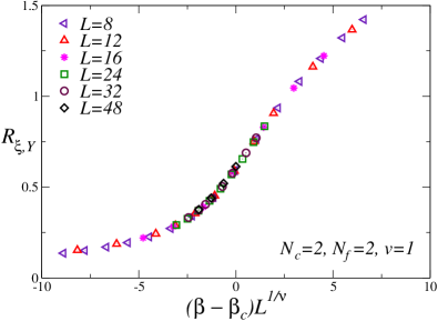
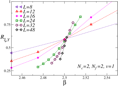
Figure 6: Data of $R_{\xi,Y}$ for $N_{c}=N_{f}=2$, $\gamma=0$ and $v=1$, versus $\beta$ (bottom) and versus $(\beta-\beta_{c})L^{1/\nu}$ (top). We use the XY critical exponent $\nu=0.6717$ and our best estimate $\beta_{c}=2.502$ of the critical point. The excellent collapse of the data (top panel) demonstrates that the transition belongs to the XY universality class.

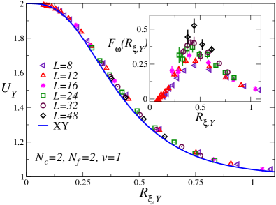
Figure 7: Estimates of $U_{Y}$ versus $R_{\xi,Y}$ for $N_{c}=N_{f}=2$, $\gamma=0$ and $v=1$. The continuous line is the XY universal curve $F(R_{\xi})$ (taken from Ref. BPV-21-coAH ). Estimates of $L^{\omega}[U_{Y}-F(R_{\xi,Y})]$ versus $R_{\xi,Y}$, using the XY correction-to-scaling exponent $\omega=0.789$, are reported in the inset. The data show a reasonable scaling behavior, which is definitely consistent with the scaling behavior (64).

For $v=1$, the estimates of the order parameter $Y_{\bm{x}}^{fg}$ defined in Eq. (13), are reported in Figs. 6 and 7. The data confirm the existence of a continuous transition at $\beta\approx 2.50$, which belongs to the U(1), or XY, universality class. Indeed, if we fit the data using the XY estimate $\nu=0.6717(1)$ (see Refs. CHPV-06 ; Hasenbusch-19 ; CLLPSSV-20 ; PV-02 ) we obtain $\beta_{c}=2.502(1)$ and an excellent collapse of the data (upper panel of Fig. 6). The best evidence that the transition belongs to the XY universality class is provided by the plot of $U_{Y}$ versus $R_{\xi,Y}$. Data approach the asymptotic universal curve $F(R_{\xi})$ corresponding to the XY universality class (the curve is taken from the appendix of Ref. BPV-21-coAH, ). Moreover, the approach to the universal XY curve, see the inset of Fig. 7, is consistent with the expected FSS scaling behavior

$$U(L,R_{\xi,Y})-F(R_{\xi,Y})\approx L^{-\omega}F_{\omega}(R_{\xi,Y})\,,$$ (64)

where $\omega$ is the leading scaling-correction exponent and $F_{\omega}(R_{\xi})$ is a scaling function that is universal apart from a multiplicative factor. If we use the XY estimate Hasenbusch-19 $\omega=0.789(4)$, we observe a reasonable scaling, again confirming that the transition is related to the breaking of the U(1) symmetry. The SU($N_{f}$) symmetry is unbroken and the indeed, correlations of the bilinear operator $Q$ are not critical (but still nonanalytic) for $v>0$, as expected, see Fig. 8.

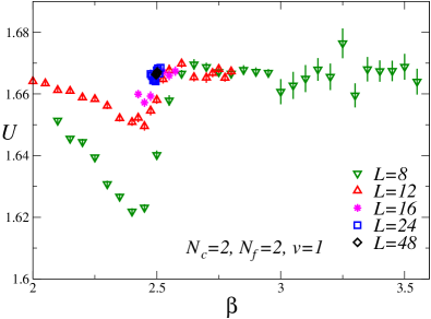
Figure 8: Data of $\xi$ (top) and $U$ (bottom) for $N_{c}=N_{f}=2$, $\gamma=0$ and $v=1$, as obtained from the correlations of the bilinear operator $Q_{\bm{x}}$. They clearly show that the correlations of the bilinear operator $Q$ do not become critical for $v>0$, as expected.

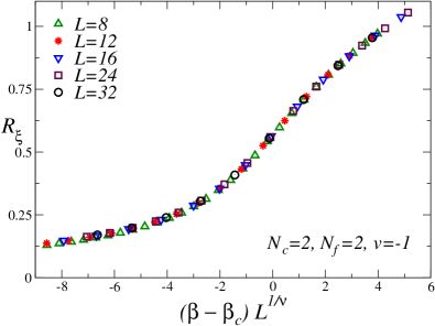
Figure 9: Plot of $R_{\xi}$ for $N_{c}=N_{f}=2$, $\gamma=0$ and $v=-1$, versus $(\beta-\beta_{c})L^{1/\nu}$, using the O(3) critical exponent Hasenbusch-19 $\nu=0.71164$ and our best estimate $\beta_{c}=2.561$ of the critical point. The excellent collapse of the data supports the O(3) critical behavior.

In Figs. 9 and 10 we report results for $v=-1$. In this case, the order parameter $Q_{\bm{x}}^{fg}$ defined Eq. (9) is critical, signalling the breaking of the SU(2) symmetry and therefore the presence of a transition that belongs to the CP¹ or O(3) universality class. In Fig. 9 we report a scaling plot of $R_{\xi}$ using  Hasenbusch-20 the O(3) estimate $\nu=0.71164(10)$ (accurate estimates of the O(3) exponents can be found in Refs. Hasenbusch-20 ; Chester-etal-20-o3 ; KP-17 ; HV-11 ; PV-02 ; CHPRV-02 ; GZ-98 ) and the estimate of the critical temperature $\beta_{c}=2.561(1)$, obtained by performing biased fits of the data, in which $\nu$ was fixed to the O(3) value. The agreement is excellent. As before, we also considered $U$ versus $R_{\xi}$. Data fall on top of the O(3) curve (it is reported in the appendix of Ref. BPV-21-coAH ) with small corrections that are consistent with Eq. (64) and the O(3) value of the scaling-correction exponent, Hasenbusch-20 $\omega=0.759(2)$. We also mention that correlations of the operator $Y_{\bm{x}}$ are not critical, as expected.

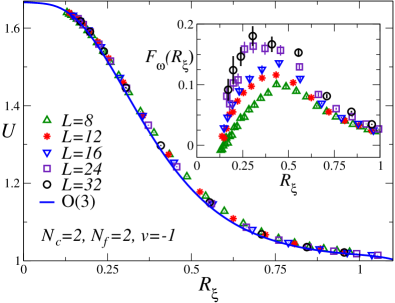
Figure 10: $U$ versus $R_{\xi}$, as obtained from the correlations of the bilinear operator $Q$, for $N_{c}=N_{f}=2$, $\gamma=0$ and $v=-1$. The data appear to approach the universal curve corresponding to the O(3) universality class  BPV-21-coAH . In the inset we report $F_{\omega}(R_{\xi})\equiv L^{\omega}[U-F(R_{\xi})]$ versus $R_{\xi}$, using the O(3) correction-to-scaling exponent Hasenbusch-20 $\omega=0.759$. The data, in particular those for the largest available lattice sizes, show a reasonably good scaling.

In conclusion, our numerical results confirm the discussion of Sec. VI.2, and are fully consistent with the phase diagram reported in Fig. 1. We expect the same qualitative behavior for any finite inverse gauge coupling $\gamma>0$.

VII.2 Results for $N_{f}>N_{c}=2$

We now present some numerical results for two large values of $N_{f}$, $N_{f}=20$ and $N_{f}=40$, to check whether the lattice model develops a critical behavior that can be associated with the charged FP of the corresponding SU($N_{c}$) gauge field theory. As we have discussed in Sec. V, the charged FP is expected to be present only if the gauge fields develop a critical dynamics. Therefore, we expect such a behavior for nonvanishing values of $\gamma$. For $\gamma=0$, the gauge fields can be integrated out and one obtains an effective scalar model for the two order parameters, whose critical behavior should be well described within the standard LGW approach without gauge fields, see App. A.

For $N_{f}=20$, we have performed simulations for two values of $\gamma$, choosing $\gamma=1$ and 3. For $\gamma=1$, we have also studied the $v$ dependence, considering $v=1$ and $v=10$. Results for $\gamma=1$ depend only weakly on $v$ and indeed, we find that both models undergo a transition for a similar values of $\beta$, $\beta_{c}\approx 1.28$. The results for the specific heat $C_{V}$ and the Binder parameter $U$ are shown in Figs. 11 and 12, respectively. They are consistent with a first-order transition: we do not observe scaling when $U$ is plotted against $R_{\xi}$ and the maximum of $U$ increases with $L$. Also the data for $\gamma=3$ and $v=1$ favor a first-order transition, see Fig. 13, at $\beta_{c}\approx 1.16$. The transition is weaker than that observed for $\gamma=1$, and indeed larger lattices are needed to observe the emergence of the typical features of first-order transitions. This is not unexpected, since the transition may become continuous for $\gamma\to\infty$, controlled by the stable FP of the matrix model (59), see Sec. VI.1.

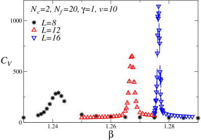
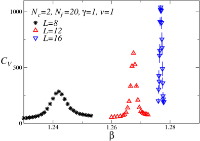
Figure 11: Data for the specific heat $C_{V}$ for $N_{c}=2$, $N_{f}=20$, $\gamma=1$, $v=10$ (top) and $v=1$ (bottom). The apparent divergence of $C_{V}$ with increasing $L$ supports a first-order transition.

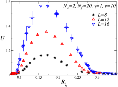
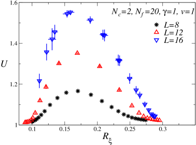
Figure 12: The Binder parameter $U$ versus the ratio $R_{\xi}$ for $N_{c}=2$, $N_{f}=20$, $\gamma=1$, $v=10$ (top) and $v=1$ (bottom). Data do not of converge and the maximum of the Binder parameter $U$ increases with increasing $L$, as expected for a first-order transition (see the discussion at the end of Sec. III).

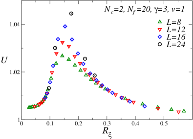
Figure 13: The Binder parameter $U$ versus the ratio $R_{\xi}$ for $N_{c}=2$, $N_{f}=20$, $v=1$, and $\gamma=3$. No scaling is observed, indicating that the transition is of first order.

As no evidence for a charged FP was found for $N_{f}=20$, we decided to study the model for an even larger number of flavors. We chose $N_{f}=40$ and performed simulations for $\gamma=0$ and 1, and also for the matrix model obtained in the limit $\gamma=\infty$ (it amounts to setting $U_{{\bm{x}},\mu}=1$ on every link). As $v$ does not play a role, we always fixed $v=1$.

For $\gamma=0$, we observe a very strong first-order transition at $\beta_{c}\approx 1.2$. Already on small lattices, there are long-living metastable states and we are not able to thermalize the system for $L\gtrsim 12$. There is apparently no FP in the model in which gauge fields are integrated out. To detect the possible presence of a charged FP, we performed simulations for a finite value of $\gamma$, choosing $\gamma=1$. Results corresponding to $8\leq L\leq 28$ are fully consistent with a continuous transition at $\beta_{c}\approx 1.18$. First, the specific heat is apparently bounded—its maximum does not increase with $L$. Second, the plot of the Binder parameter versus $R_{\xi}$, see Fig. 14, shows a reasonably good scaling. In particular, the maximum of the Binder parameter does not increase with $L$. On the contrary, it apparently decreases with increasing sizes (we find $U_{\rm max}\approx 1.06$,1.04 for $L=12$ and 28, respectively), a phenomenon that is not consistent with a first-order transition. The strong peak in the Binder parameter can be interpreted as a crossover effect, due to the first-order transition line that is expected to be present for smaller values of $\gamma$ and that ends in the transition point at $\beta_{c}\approx 1.2$, $\gamma=0$.

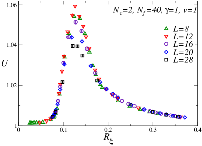
Figure 14: The Binder parameter $U$ versus the ratio $R_{\xi}$ for $N_{c}=2$, $N_{f}=40$, $v=1$, and $\gamma=1$. The data appear to converge to a scaling curve with increasing $L$, consistently with a continuous transition.

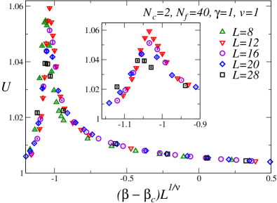
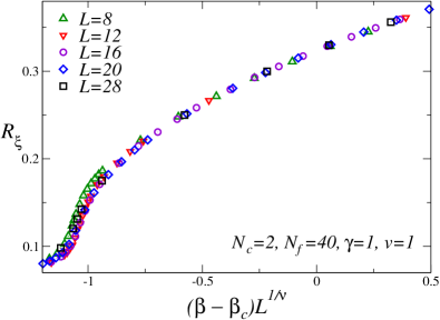
Figure 15: Binder paramer $U$ (top) and correlation-length ratio $R_{\xi}$ (bottom) versus $X=(\beta-\beta_{c})L^{1/\nu}$ for $N_{c}=2$, $N_{f}=40$, $v=1$, and $\gamma=1$. We set $\beta_{c}=1.1864$ and $\nu=0.74$. The inset in the upper panel gives a more detailed view of the behavior of the Binder parameter for $-1.2\leq X\leq-0.8$, the values of $X$ where $U$ has a peak.

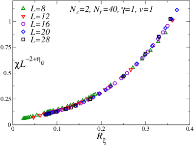
Figure 16: Estimates of $L^{\eta_{Q}-2}\chi$ versus $R_{\xi}$, for $N_{c}=2$, $N_{f}=40$, $v=1$, and $\gamma=1$. We set $\eta_{Q}=0.89$.

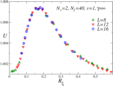
Figure 17: The Binder parameter $U$ versus the ratio $R_{\xi}$ for $N_{c}=2$, $N_{f}=40$, $v=1$, and $\gamma=\infty$ (ungauged matrix model).

As the transition for $\gamma=1$ is apparently continuous, it is interesting to determine the corresponding critical exponents. The exponent $\nu$ has been determined by fitting $R_{\xi}$ to $f(X)$, with $X=(\beta-\beta_{c})L^{1/\nu}$. We have parameterized the function $f(X)$ with an order-$n$ polynomial (stable results are obtained for $n\gtrsim 15$). We have performed several fits, including each time only data satisfying $L\geq L_{\rm min}$ (we used $L_{\rm min}=8,12,16$). Moreover, as corrections appear to be stronger in the region where $U$ has a peak, we also investigated how results change if only data satisfying $R_{\xi}\geq 0.20$ are considered. The results of these analyses are consistent with

$$\beta_{c}=1.1864(1)\,,\qquad\nu=0.74(2)\,.$$ (65)

In Fig. 15 we report the plots of $U$ and $R_{\xi}$ versus $X$, using the estimates (65). We observe good scaling, except for $X\lesssim-0.8$, where $U$ has a peak. Note that $\nu>2/3$, and thus the result is consistent with a finite specific heat at the transition for $L\to\infty$. We have also estimated the exponent $\eta_{Q}$ that characterizes the behavior of the susceptibility, $\chi\sim L^{2-\eta_{Q}}$ at the critical point. To estimate $\eta_{Q}$ we have fitted $\log\chi$ to $(2-\eta_{Q})\log L+g_{\chi}(R_{\xi})$, using a polynomial parametrization for the function $g(x)$. We find

$$\eta_{Q}=0.89(3).$$ (66)

Scaling is excellent, as shown in Fig. 16.

The transition we have identified for $\gamma=1$ can be naturally associated with the charged FP of the SU($N_{c}$) field theory (V). A conclusive proof would require a detailed analysis of the gauge correlations. However, note that such a FP disappears as $\gamma$ is decreased towards zero and is not present in the matrix model in which the gauge fields are integrated out, confirming that gauge fields do indeed play a role. It would be interesting to compare the estimates of the critical exponents with the large-$N_{f}$ predictions computed in the gauge field theory—these results are not available at present—as this would provide a more quantitative check of the identification.

As a final check, we have studied the behavior of the model for $\gamma=\infty$, to exclude that the observed behavior for $\gamma=1$ is simply a crossover effect due to the presence of a continuous transition in the infinite-$\gamma$ matrix model. We recall that the model in the $\gamma\to\infty$ limit becomes equivalent to the lattice scalar model (59), which can have continuous transitions for sufficiently large $N_{f}$, and in particular for $N_{f}=40$, see Sec. VI.1. MC simulations of the ungauged matrix model provide evidence of a phase transition for $\beta_{c}\approx 1.00$. In Fig. 17 we report $U$ versus $R_{\xi}$. We observe excellent scaling, indicating that the transition is continuous. The curve we obtain is quite different from the one obtained for $\gamma=1$, see Fig. 14. For instance, in the matrix model the maximum of $U$ is approximately 1.007, which is significantly smaller than the value obtained for $\gamma=1$, see the inset in the upper panel of Fig. 15.

We have also determined the exponents for the matrix model. Although we only have data for $8\leq L\leq 16$, scaling corrections are small. Analyzing the data as we did for $\gamma=1$, we obtain

$$\beta_{c}=1.0079(4)\,,\quad\nu=0.975(5)\,,\quad\eta_{Q}=1.147(5)\,.$$ (67)

Note that $\eta_{Q}$ is the critical exponent associated with the composite operator $Q$ and it should not be confused with the exponent $\eta$ that characterizes the critical behavior of the correlations of the fundamental field $\Phi^{af}$, that are well defined in the ungauged model. The estimates of the exponents are very different from those obtained for finite $\gamma$, again excluding that the results for $\gamma=1$ are a crossover due to the presence of a continuous transition in the ungauged matrix model.

VIII Conclusions

We have investigated how nonabelian global and gauge symmetries shape the phase diagram of 3D lattice gauge theories. We consider a model with SU($N_{c}$) local invariance and U($N_{f}$) global invariance, in which the scalar fields transform under the fundamental representation of both groups. We use a standard formulation with nearest-neighbor couplings Wilson-74 , considering the most general quartic scalar potential compatible with the given global and gauge symmetry, cf. Eq. (4). We determine the low-temperature Higgs phases and the nature of the phase transitions, as a function of the parameter $v$ entering the quartic potential, defined in Eq. (7). This study extends the one reported in Refs. BPV-19 ; BPV-20-su for maximally symmetric scalar potentials, corresponding to fixing $v=0$. We show that such an extension to multiparameter quartic parameters give rise to various notable scenarios, characterized by different low-temperature Higgs phases.

The analysis of the minimum-energy configurations allows us to determine the main features of the phase diagram. We determine the ordered Higgs phases, their global and gauge symmetry-breaking pattern, and the nature of the transition lines between the various phases. These features depend on the scalar-potential parameter $v$ and on the number of colors and flavors, $N_{c}$ and $N_{f}$, respectively. We observe qualitative differences between the cases $N_{c}=2$ and $N_{c}>2$, and the cases $N_{f}<N_{c}$, $N_{f}=N_{c}$ and $N_{f}>N_{c}$, as sketched in Figs. 1, 2, 3, 4, and 5. In particular, for $N_{f}\geq N_{c}$ the phase diagram presents two distinct Higgs phases, associated with different global and gauge symmetry-breaking patterns.

To check the theoretical arguments, we performed numerical MC simulations for $N_{c}=2$. For $v=0$ and any $N_{f}$, the model is invariant under a larger symmetry group, namely Sp($N_{f}$)/${\mathbb{Z}}_{2}$. Therefore, a first-order transition line is expected on the $v=0$ axis for sufficiently large values of $\beta$, separating two different low-temperature ordered phases corresponding to $v>0$ and $v<0$, respectively, see Figs. 1 and 2. In particular, for $N_{f}=2$, the global symmetry of the model with $v=0$ enlarges to $\hbox{Sp(2)}\simeq\hbox{O(5)}$, leading to the emergence of an O(5) multicritical point, where the continuous transition lines extending within the regions $v>0$ and $v<0$ meet. According to the theoretical arguments reported in Secs. IV and VI, for $v>0$ the transition line belongs to the XY universality class—the corresponding order parameter is the determinant of the scalar fields, see Eqs. (12) and (13)— while, for $v<0$, it belongs to the O(3) universality class, being associated with the condensation of the gauge-invariant bilinear operator defined in Eq. (9). The FSS analyses of the numerical data support these theoretical predictions, thus conferming the phase diagram sketched in Fig. 1.

We also present results for larger values of $N_{f}$, focusing on the phase behavior for $v>0$, whose nature is unknown, see Fig. 2 and the corresponding discussion in Sec. VI. In particular, we address the question of the existence of transitions that can be associated with the stable charged FP that is present in the scalar SU(2) gauge field theory—the corresponding Lagrangian is reported in Eq. (V)—for large values of $N_{f}$.

This issue has been recently addressed in the Abelian-Higgs field theory characterized by a local U(1) and a global U($N_{f}$) symmetry. Field theory predicts the existence of a stable charged FP for a sufficiently large number of components HLM-74 ; DHMNP-81 ; FH-96 ; YKK-96 ; MZ-03 ; KS-08 ; IZMHS-19 . In the $\epsilon$-expansion approach, such a FP only exists for $N_{f}>N^{*}_{f}(d)$, where $d$ is the space dimension. In $d=4$ dimensions, $N^{*}_{f}(4)\approx 183$. However, corrections in the expansion in powers of $\epsilon=4-d$ are large and four-loop results provide a significantly smaller estimate in $d=3$, $N^{*}_{f}(3)\approx 12$. Recent numerical work on the 3D lattice Abelian-Higgs model with noncompact gauge fields BPV-21-nc identified a transition line along which critical exponents are in quantitative agreement with the field theory large-$N_{f}$ predictions: these transitions can therefore be associated with the charged FP. These results provided the estimate BPV-21-nc $N^{*}_{f}(3)=7(2)$, confirming that the large value in four dimensions, $N^{*}_{f}(4)\approx 183$, is quantitatively not relevant for the 3D case. It is worth noting that the charged FP is also relevant for some transitions occuring in the compact Abelian-Higgs model when the scalar matter has a charge larger than one BPV-20-hc .

As it occurs in the scalar U(1) field theory, SU($2$) field theories have a stable charged FP in the region $v>0$ for $N_{f}>N^{*}_{f}(d)$. Close to four dimensions, $N^{*}(d)$ is very large, indeed $N^{*}_{f}(4)\approx 376$, see Sec. V. However, it is conceivable that the critical value $N^{*}_{f}(3)$ in three dimensions is significantly smaller than the four-dimensional one, as it occurs in the Abelian-Higgs models. To check whether 3D SU(2) lattice models undergo transitions associated with the field-theory charged FP, we have performed simulations for two large number of components, $N_{f}=20$ and $N_{f}=40$. For $N_{f}=20$ we have only evidence of first-order transitions. A continuous transition is instead observed for $N_{f}=40$, $\gamma=1$, and $v=1$. The transition becomes of first order in the infinite-gauge coupling limit ($\gamma\to 0$), in which gauge fields can be integrated out, confirming that the gauge dynamics is relevant for the existence of the continuous transition. This leads us to conjecture that the continuous transition observed for $N_{f}=40$ and finite $\gamma>0$ is associated with the charged FP of the SU($N_{c}$) field theory with Lagrangian (V). If the association is correct, our results allow us to estimate $N^{*}_{f}$ in three dimensions. The critical value $N^{*}_{f}(3)$ is large, $20<N^{*}_{f}(3)<40$, but still significantly smaller that the four-dimensional value.

It is clear that significant additional work is needed to fully clarify this issue. On the numerical side, a detailed analysis of gauge correlations at the transition is clearly required, while on the field-theory side it would be important to have quantitative predictions for universal quantities, for instance, for the critical exponents. Indeed, this would allow us to perform a more quantitative comparison between the numerical results obtained in the simulation of the lattice gauge model and the corresponding SU($N_{c}$) field theory predictions. A complete understanding of this issue is fundamental to clarify if and how the nonabelian gauge field theory can be realized in 3D statistical models sharing the same global and local symmetries.

Acknowledgement. Numerical simulations have been performed using the CSN4 cluster of the Scientific Computing Center at INFN-PISA and the Green Data Center of the University of Pisa.

Appendix A Effective model for $N_{c}=2$

In this Appendix we briefly discuss the effective scalar model that can be obtained for $\gamma=0$ be integrating out the gauge fields. We will use the results of Ref. BRT-81 for SU($N$) link integrals. We define

$$S^{ab}=-{1\over 2}N_{f}\beta\sum_{f}\Phi_{{\bm{x}}+\hat{\mu}}^{af}(\Phi^{bf}_{\bm{x}})^{*}$$ (68)

and the invariant combination

$$K_{{\bm{x}},\mu}=\hbox{Tr }SS^{\dagger}+\hbox{det}S+\hbox{det}S^{\dagger}$$ (69)

$$\quad={1\over 4}N_{f}\beta^{2}+{1\over 4}N_{f}^{2}\beta^{2}\times$$

$$\qquad\sum_{fg}(Q^{fg}_{{\bm{x}}+\hat{\mu}}Q^{fg}_{\bm{x}}+{1\over 2}\bar{Y}^{fg}_{{\bm{x}}+\hat{\mu}}Y^{fg}_{\bm{x}}+{1\over 2}Y^{fg}_{{\bm{x}}+\hat{\mu}}\bar{Y}^{fg}_{\bm{x}}).$$

Then, we obtain

$$\int[dU]e^{-\beta H_{K}}=C\exp\sum_{{\bm{x}},\mu}\ln[I_{1}(2K_{{\bm{x}},\mu})/\sqrt{K_{{\bm{x}},\mu}}],$$ (70)

where $C$ is an irrelevant constant and $I_{1}(x)$ is a modified Bessel function. Since

$$\hbox{Tr }(\Phi^{\dagger}\Phi)^{2}=\hbox{Tr }Q^{2}-{1\over N_{f}}=\hbox{Tr }\bar{Y}Y+1-{1\over N_{f}},$$ (71)

we see that, for any $N_{f}$, in the absence of the gauge coupling, the gauge model is equivalent to a matrix model for the order parameters $Q$ and $Y$. Note also that $K_{{\bm{x}},\mu}$ can be expressed in terms of the Sp($N_{f}$) order parameter defined in Ref. BPV-20-su , explicitly showing the larger symmetry of the model for $v=0$.

We can also use these expressions to discuss the large-$\beta$ limit. In this case we have translation invariance—the fields do not depend on ${\bm{x}}$. If we use the singular value decomposition (24), we find that $K$ becomes independent of the scalar fields, namely

$$K={\beta^{2}N_{f}^{2}\over 4}(w_{1}^{2}+w_{2}^{2})^{2}={\beta^{2}N_{f}^{2}\over 4}.$$ (72)

This result proves that for $v=0$ and $\beta\to\infty$ the scalar fields are uniformly distributed, as already shown in Ref. BPV-20-su . Moreover, the scalar kinetic term is irrelevant in determining the Higgs phases at low temperature: they are uniquely fixed by the scalar potential.

Appendix B Monte Carlo simulations

We performed MC simulations on cubic lattices with periodic boundary conditions. We used two different updates of the complex scalar field $\Phi^{af}$. The first one is a standard Metropolis update Metropolis:1953am that rotates two randomly chosen elements of $\Phi_{\bm{x}}^{ab}$ (denoted by $\phi_{1}$ and $\phi_{2}$ in the following). More precisely the proposed update is

$$\phi^{\prime}_{1} =\cos\theta_{1}e^{i\theta_{2}}\phi_{1}+\sin\theta_{1}e^{i\theta_{3}}\phi_{2}$$ (73)

$$\phi^{\prime}_{2} =-\sin\theta_{1}e^{i\theta_{2}}\phi_{1}+\cos\theta_{1}e^{i\theta_{3}}\phi_{2}\,,$$

where the angles $\theta_{i}$ are uniformly distributed in $[-\alpha,\alpha]$, and the value of $\alpha$ are chosen to obtain an acceptance of approximately 30%. In the second update we propose the change

$$\Phi^{\prime}_{\bm{x}}=\frac{2\mathrm{Re}\Tr(\Phi^{\dagger}_{\bm{x}}S_{\bm{x}})}{\Tr(S^{\dagger}_{\bm{x}}S_{\bm{x}})}S_{\bm{x}}-\Phi_{\bm{x}}\,,$$ (74)

where $S_{\bm{x}}$ is the matrix

$$S_{\bm{x}}=\sum_{\mu}(U_{{\bm{x}},\mu}\Phi_{{\bm{x}}+\hat{\mu}}+U^{\dagger}_{{\bm{x}}-\hat{\mu},\mu}\Phi_{{\bm{x}}-\hat{\mu}})\,.$$ (75)

Such a deterministic update satisfies detailed balance (since it is involutive), and for $v=0$ would be an overrelaxation step Creutz:1987xi . For $v\neq 0$ this move is accepted or rejected using a standard Metropolis test, and for the parameters used in this work a typical value of the corresponding acceptance rate is 90%. Link variables were updated using the Metropolis algorithm, with the proposed update $U_{{\bm{x}},\mu}\to VU_{{\bm{x}},\mu}$, where $V$ is an SU($N_{c}$) matrix close to the identity and $V$ or $V^{{\dagger}}$ were used with a 50% probability to ensure detailed balance. Also in this case the maximal distance of $V$ from the identity matrix was chosen in such a way to have an average 30% acceptance ratio.

We call lattice iteration a series of 10 lattice sweeps in which we sequentially update the scalar field on all the sites and the gauge field on all the links. In 9 lattice sweeps we use the pseudo-overrelaxed update with proposal (74), while in 1 sweep we use the update based on the proposal (73). This ratio of 1 to 9 was kept fixed for all the cases studied in this work, since we verified the autocorrelation times to be small enough for our purposes, and we did not pursued any further parameter optimization.

Measures where performed after every lattice iteration, and for the largest lattice sizes typical statistics of our runs were $\approx 3\times 10^{6}$ measures in the case of two-flavor models, and $\approx 8\times 10^{5}$ and $\approx 4\times 10^{5}$ for $N_{f}=20$ and $N_{f}=40$ respectively. To analyze data and estimate error bars we used standard blocking and jackknife techniques, and the maximum blocking size adopted was of the order of $10^{3}$ data.

References

- (1) K. G. Wilson, Confinement of quarks, Phys. Rev. D 10, 2445 (1974).
- (2) J. Zinn-Justin, Quantum Field Theory and Critical Phenomena, fourth edition (Clarendon Press, Oxford, 2002).
- (3) S. Weinberg, The Quantum Theory of Fields, (Cambridge University Press, 2005).
- (4) F. J. Wegner. Duality in generalized Ising models and phase transitions without local order parameters J. Math. Phys. 12, 2259 (1971).
- (5) P. W. Anderson, Basic Notions of Condensed Matter Physics, (The Benjamin/Cummings Publishing Company, Menlo Park, California, 1984).
- (6) S. Sachdev, Topological order, emergent gauge fields, and Fermi surface reconstruction, Rep. Prog. Phys. 82, 014001 (2019).
- (7) H. Georgi and S. L. Glashow, Unified weak and electromagnetic interactions without neutral currents, Phys. Rev. Lett. 28, 1494 (1972).
- (8) K. Osterwalder and E. Seiler, Gauge Field Theories on the Lattice, Ann. Phys. (NY) 110, 440 (1978).
- (9) E. Fradkin and S. Shenker, Phase diagrams of lattice gauge theories with Higgs fields, Phys. Rev. D 19, 3682 (1979).
- (10) S. Dimopoulos, S. Raby, and L. Susskind, Light Composite Fermions, Nucl. Phys. B 173, 208 (1980).
- (11) C. Borgs and F. Nill, The Phase Diagram of the Abelian Lattice Higgs Model. A Review of Rigorous Results, J. Stat. Phys. 47, 877 (1987).
- (12) C. Bonati, A. Pelissetto, and E. Vicari, Phase Diagram, Symmetry Breaking, and Critical Behavior of Three-Dimensional Lattice Multiflavor Scalar Chromodynamics, Phys. Rev. Lett. 123, 232002 (2019).
- (13) C. Bonati, A. Pelissetto, and E. Vicari, Three-dimensional lattice multiflavor scalar chromodynamics: Interplay between global and gauge symmetries, Phys. Rev. D 101, 034505 (2020).
- (14) C. Bonati, A. Pelissetto, and E. Vicari, Three-dimensional phase transitions in multiflavor scalar SO() gauge theories, Phys. Rev. E 101, 062105 (2020).
- (15) S. Sachdev, H. D. Scammell, M. S. Scheurer, and G. Tarnopolsky, Gauge theory for the cuprates near optimal doping, Phys. Rev. B 99, 054516 (2019).
- (16) H. D. Scammell, K. Patekar, M. S. Scheurer, and S. Sachdev, Phases of SU(2) gauge theory with multiple adjoint Higgs fields in 21 dimensions, Phys. Rev. B 101, 205124 (2020).
- (17) C. Bonati, A. Franchi, A. Pelissetto, and E. Vicari, Three-dimensional lattice SU() gauge theories with multiflavor scalar fields in the adjoint representation, Phys. Rev B 114, 115166 (2021).
- (18) S. Nadkarni, The SU(2) Adjoint Higgs Model in Three dimensions, Nucl. Phys. B 334, 559 (1990).
- (19) K. Kajantie, K. Rummukainen and M. E. Shaposhnikov, A Lattice Monte Carlo study of the hot electroweak phase transition, Nucl. Phys. B 407, 356 (1993).
- (20) W. Buchmüller and O. Philipsen, Phase structure and phase transition of the SU(2) Higgs model in three-dimensions, Nucl. Phys. B 443, 47 (1995).
- (21) K. Kajantie, M. Laine, K. Rummukainen, and M. E. Shaposhnikov, Is there a hot electroweak phase transition at ?, Phys. Rev. Lett. 77, 2887 (1996).
- (22) A. Hart, O. Philipsen, J. D. Stack, and M. Teper, On the phase diagram of the SU(2) adjoint Higgs model in (2+1)-dimensions, Phys. Lett. B 396, 217 (1997).
- (23) C. Bonati, A. Pelissetto, and E. Vicari, Lattice Abelian-Higgs models with noncompact gauge field, Phys. Rev. B 103, 085104 (2021).
- (24) C. Bonati, A. Pelissetto, and E. Vicari, Higher-charge three-dimensional compact lattice Abelian-Higgs models, Phys. Rev. E 102, 062151 (2020).
- (25) A. Pelissetto and E. Vicari, Critical phenomena and renormalization group theory, Phys. Rep. 368, 549 (2002).
- (26) M. S. S. Challa, D. P. Landau, and K. Binder, Finite-size effects at temperature-driven first-order transitions Phys. Rev. B 34, 1841 (1986).
- (27) K. Vollmayr, J. D. Reger, M. Scheucher, and K. Binder, Finite size effects at thermally-driven first order phase transitions: A phenomenological theory of the order parameter distribution Z. Phys. B 91 113 (1993).
- (28) P. Calabrese, P. Parruccini, A. Pelissetto, and E. Vicari, Critical behavior of O(2)O()-symmetric models, Phys. Rev. B 70, 174439 (2004).
- (29) A. Pelissetto and E. Vicari, Three-dimensional ferromagnetic CPN-1 models, Phys. Rev. E 100, 022122 (2019).
- (30) A. Pelissetto and E. Vicari, Multicomponent compact Abelian-Higgs lattice models, Phys. Rev. E 100, 042134 (2019).
- (31) A. Pelissetto and E. Vicari, Large- behavior of three-dimensional lattice CPN-1 models, J. Stat. Mech. (2020) 033209.
- (32) A. Nahum, J. T. Chalker, P. Serna, M. Ortuño, and A. M. Somoza, 3D Loop Models and the CPN-1 Sigma Model, Phys. Rev. Lett. 107, 110601 (2011).
- (33) A. Nahum, J. T. Chalker, P. Serna, M. Ortuño, and A. M. Somoza, Phase transitions in three-dimensional loop models and the CPN-1 sigma model, Phys. Rev. B 88, 134411 (2013).
- (34) R. K. Kaul and A. W. Sandvik, Lattice Model for the SU() Neèl to valence-bond solid quantum phase transition at large , Phys. Rev. Lett. 108, 137201 (2012)
- (35) B. Ihrig, N. Zerf, P. Marquard, I. F. Herbut, and M. M. Scherer, Abelian Higgs model at four loops, fixed-point collision and deconfined criticality, Phys. Rev. B 100, 134507 (2019).
- (36) M. Moshe and J. Zinn-Justin, Quantum field theory in the large limit: A review, Phys. Rep. 385, 69 (2003).
- (37) B. I. Halperin, T. C. Lubensky, and S. K. Ma, First-Order Phase Transitions in Superconductors and Smectic-A Liquid Crystals, Phys. Rev. Lett. 32, 292 (1974).
- (38) P. Di Vecchia, A. Holtkamp, R. Musto, F. Nicodemi, and R. Pettorino, Lattice CPN-1 models and their large- behaviour, Nucl. Phys. B 190, 719 (1981).
- (39) R. Folk and Y. Holovatch, On the critical fluctuations in superconductors, J. Phys. A 29, 3409 (1996).
- (40) V. Yu. Irkhin, A. A. Katanin, and M. I. Katsnelson, expansion for critical exponents of magnetic phase transitions in the model for , Phys. Rev. B 54, 11953 (1996).
- (41) R. K. Kaul and S. Sachdev, Quantum criticality of U(1) gauge theories with fermionic and bosonic matter in two spatial dimensions, Phys. Rev. B 77, 155105 (2008).
- (42) R. Cipolloni, Sapienza Master thesis (2022); S. Rulli, Master thesis, University of Pisa (2022).
- (43) R. D. Pisarski and F. Wilczek, Remarks on the chiral phase transition in chromodynamics, Phys. Rev. D 29, 338 (1984).
- (44) A. Butti, A. Pelissetto, and E. Vicari, On the nature of the finite-temperature transition in QCD, J. High Energy Phys. 08, 029 (2003).
- (45) A. Pelissetto and E. Vicari, Relevance of the axial anomaly at the finite-temperature chiral transition in QCD, Phys. Rev. D 88, 105018 (2013).
- (46) P. Calabrese and P. Parruccini, Five-loop epsilon expansion for U()U() models: finite-temperature phase transition in light QCD, J. High Energy Phys. 05 (2004) 018.
- (47) H. Georgi, Weak interactions and modern particle theory, (The Benjamin/Cummings Publishing Company, Menlo Park, California, 1984).
- (48) P. Arnold and L. G. Yaffe, The expansion and the electroweak phase transition, Phys. Rev. D 49, 3003 (1994).
- (49) P. S. Bhupal Dev and A. Pilaftsis, Maximally Symmetric Two Higgs Doublet Model with Natural Standard Model Alignment, JHEP 1412, 024 (2014); (Erratum) JHEP 1511, 147 (2015).
- (50) C. Wang, A. Nahum, M. A. Metlitski, C. Xu, and T. Senthil, Deconfined Quantum Critical Points: Symmetries and Dualities, Phys. Rev. X 7, 031051 (2017).
- (51) P. Calabrese, A. Pelissetto, and E. Vicari, Multicritical behavior of -symmetric systems, Phys. Rev. B 67, 054505 (2003).
- (52) M. Hasenbusch, A. Pelissetto, and E. Vicari, Instability of the O(5) critical behavior in the SO(5) theory of high- superconductors, Phys. Rev. B 72 014532 (2005).
- (53) M. Campostrini, M. Hasenbusch, A. Pelissetto, and E. Vicari, Theoretical estimates of the critical exponents of the superfluid transition in 4He by lattice methods, Phys. Rev. B 74, 144506 (2006).
- (54) M. Hasenbusch, Monte Carlo study of an improved clock model in three dimensions, Phys. Rev. B 100, 224517 (2019).
- (55) S. M. Chester, W. Landry, J. Liu, D. Poland, D. Simmons-Duffin, N. Su, and A. Vichi, Carving out OPE space and precise O(2) model critical exponents, J. High Energy Phys. 06, 142 (2020).
- (56) C. Bonati, A. Pelissetto and E. Vicari, Lattice gauge theories in the presence of a linear gauge-symmetry breaking, Phys. Rev. E 104, 014140 (2021).
- (57) M. Hasenbusch, Monte Carlo study of a generalized icosahedral model on the simple cubic lattice, Phys. Rev. B 102, 024406 (2020).
- (58) S. M. Chester, W. Landry, J. Liu, D. Poland, D. Simmons-Duffin, N. Su, and A. Vichi, Bootstrapping Heisenberg magnets and their cubic instability, arXiv:2011.14647.
- (59) M. V. Kompaniets and E. Panzer, Minimally subtracted six-loop renormalization of -symmetric theory and critical exponents, Phys. Rev. D 96, 036016 (2017).
- (60) M. Hasenbusch and E. Vicari, Anisotropic perturbations in 3D O(N) vector models, Phys. Rev. B 84, 125136 (2011).
- (61) M. Campostrini, M. Hasenbusch, A. Pelissetto, P. Rossi, and E. Vicari, Critical exponents and equation of state of the three-dimensional Heisenberg universality class, Phys. Rev. B 65, 144520 (2002).
- (62) R. Guida and J. Zinn-Justin, Critical exponents of the -vector model, J. Phys. A 31, 8103 (1998).
- (63) R. Brower, P. Rossi, and C.-I.Tan, The external field problem for QCD, Nucl. Phys. B 190, 699 (1981).
- (64) N. Metropolis, A. W. Rosenbluth, M. N. Rosenbluth, A. H. Teller, and E. Teller, Equation of state calculations by fast computing machines, J. Chem. Phys. 21, 1087 (1953).
- (65) M. Creutz, Overrelaxation and Monte Carlo Simulation, Phys. Rev. D 36, 515 (1987).