Asynchronous Upper Confidence Bound Algorithms for Federated Linear Bandits

Abstract

Linear contextual bandit is a popular online learning problem. It has been mostly studied in centralized learning settings. With the surging demand of large-scale decentralized model learning, e.g., federated learning, how to retain regret minimization while reducing communication cost becomes an open challenge. In this paper, we study linear contextual bandit in a federated learning setting. We propose a general framework with asynchronous model update and communication for a collection of homogeneous clients and heterogeneous clients, respectively. Rigorous theoretical analysis is provided about the regret and communication cost under this distributed learning framework; and extensive empirical evaluations demonstrate the effectiveness of our solution.

Keywords: Contextual bandit, Federated learning, Asynchronous Communication

1 Introduction

As a popular online learning problem, linear contextual bandit has been used for a variety of applications, including recommender systems (Li et al., 2010a), display advertisement (Li et al., 2010b) and clinical trials (Durand et al., 2018). While most existing solutions are designed under a centralized setting (i.e., data is readily available at a central server), in response to the increasing application scale and public concerns of privacy, there is a growing demand to keep data decentralized and push the learning of bandit models to the client side. Federated learning has recently emerged as a promising setting for decentralized machine learning (Konečnỳ et al., 2016). Since its debut in 2017, there have been many variations for different applications (Yang et al., 2019). However, most existing works study offline supervised learning problems (Li et al., 2019b; Zhao et al., 2018), which only concerns optimization convergence over a fixed dataset. How to perform federated bandit learning remains under-explored, and is the main focus of this paper.

Analogous to its offline counterpart, the goal of federated bandit learning is to minimize the cumulative regret incurred by $N$ clients during their online interactions with the environment over time horizon $T$, while keeping each client’s raw data local. Take recommender systems as an example, where the clients correspond to the edge devices that directly interact with user by making recommendations and receiving feedbacks. Unlike centralized setting where observations from all clients are immediately transmitted to the server to learn a single model, in federated bandit learning, each client makes recommendations based on its local model, with occasional communication for collaborative model estimation.

Several new challenges arise in this problem setting. The first is the conflict between the need of timely data/model aggregation for regret minimization and the need of communication efficiency, since communication is the main bottleneck for many distributed application scenarios, e.g., communication in a network of mobile devices can be slower than local computation by several orders of magnitude (Huang et al., 2013). A well-designed communication strategy becomes vital to strike the balance. In addition, the clients often have various response time and even occasional unavailability in reality, due to the differences in their computational and communication capacities. This hampers global synchronization employed in existing federated bandit solutions (Wang et al., 2019; Dubey and Pentland, 2020), which requires the server to first send a synchronization signal to all clients, wait and collect their returned local updates, and finally send the aggregated update back to every client. Second, it is very restrictive to only assume homogeneous clients, i.e., they solve the same learning problem. Studying heterogeneous clients with distinct learning problems has a greater potential in practice. This is referred to as “non-IIDness" of data in the context of federated learning, e.g., the difference in $\mathcal{P}_{i}(\mathbf{x},y)=\mathcal{P}_{i}(\mathbf{x})\mathcal{P}_{i}(y|\mathbf{x})$ is caused by each client $i\in[N]$ serving a particular user or group of users, a particular geographic region, or a particular time period. Apparently, it is also unreasonable to assume every client has equal amount of new observations, which however is assumed in existing works.

To address the first challenge, we propose an asynchronous event-triggered communication framework for federated linear bandit. Communication with a client happens only when the last communicated update to the client becomes irrelevant to the latest one; and we prove only by then effective regret reduction can be expected in this client because of the communication. Under this asynchronous communication, each client sends local update to and receives aggregated update from the server independently from other clients, with no need for global synchronization. This improves our method’s robustness against possible delays and temporary unavailability of clients. It also brings in reduced communication cost when the clients have distinct availability of new observations, because global synchronization requires every client in the learning system to send its local update despite the fact that some clients can have very few new observations since last synchronization.

To address the second challenge, we design algorithms for federated linear bandit with both “IIDness" and “non-IIDness" based on the proposed communication framework. We consider two different assumptions on the reward functions. First, all the clients share a common reward function i.e., a single model is learned for all clients. Second, each client has a distinct reward function with mutual dependence captured by globally shared components in the unknown parameter, which resembles federated multi-task learning (Smith et al., 2017). We rigorously prove the upper bounds of accumulative regret and communication cost for the proposed algorithms in these two settings, and conduct extensive empirical evaluations to demonstrate the effectiveness of our proposed framework.

2 Related Works

Most existing bandit solutions assume a centralized learning setting, where data is readily available at a central server. Classical linear bandit algorithms, like LinUCB (Li et al., 2010a; Abbasi-Yadkori et al., 2011) and LinTS (Agrawal and Goyal, 2013; Abeille and Lazaric, 2017) only concern a single learning agent. Multi-agent bandits mostly focus on customizing algorithms that leverage relationships among the agents for collaborative learning (Cesa-Bianchi et al., 2013; Wang et al., 2019; Gentile et al., 2014; Cesa-Bianchi et al., 2013; Wu et al., 2016; Li et al., 2021), but the data about all agents is still on the central server.

Distributed bandit (Korda et al., 2016; Wang et al., 2019; Dubey and Pentland, 2020) is the most relevant to ours, where designing an efficient communication strategy is the main focus. Existing algorithms mainly differ in the relations of learning problems solved by the agents (i.e., identical vs., clustered) and the type of communication network (i.e., peer-to-peer (P2P) vs., star-shaped). Korda et al. (2016) studied two problem settings with a P2P communication network: 1) all the agents solve a common linear bandit problem, and 2) the problems are clustered. However, they only tried to reduce per-round communication, and thus the communication cost is still linear over time. Two follow-up studies considered the setting where all agents solve a common problem and interact with the environment in a round-robin fashion (Wang et al., 2019; Dubey and Pentland, 2020). Similar to our work, they also used event-triggered communications to obtain a sub-linear communication cost over time. In particular, Wang et al. (2019) considered a star-shaped network and proposed a synchronous communication protocol for all clients to exchange their latest observations under the central server’s control. Dubey and Pentland (2020) extended this synchronous protocol to differentially private LinUCB algorithms under both star-shaped and P2P network.

There is also a rich literature in distributed machine learning/federated learning (McMahan et al., 2017; Li et al., 2019b) that studies offline optimization problems. However, as we mentioned earlier, due to the fundamental difference in the learning objectives, they are not applicable to our problem. Specifically, their main focus is to collaboratively learn a good point estimate over a fixed dataset, i.e., convergence to the minimizer with fewer communications, while the focus of federated bandit learning is collaborative confidence interval estimation for efficient regret reduction, which requires exploration of the unknown data. This is also reflected by the difference in the triggering event designs. For distributed offline optimization, triggering event measuring the change in the learned parameters suffices (Kia et al., 2015; Yi et al., 2018; George and Gurram, 2020), while for federated bandit learning, triggering event needs to measure change in the volume of the confidence region, i.e., uncertainty in the problem space. This adds serious challenges in the design and analysis of the triggering events. In addition, for linear bandit problems, thanks to the existence of the closed-form solution, there is no need to use gradient-based optimization methods like FedAvg (McMahan et al., 2017), because compared with transmitting the sufficient statistics, it only costs a lot more communication overhead without bringing in any gain in regret minimization.

3 Methodology

In this section, we establish the asynchronous event-triggered communication framework for federated linear bandit, and propose two UCB-type algorithms under different assumptions about the clients’ reward functions, followed by our theoretical analysis of their regret and communication cost.

3.1 Problem Formulation

Consider a learning system with 1) $N$ clients responsible for taking actions and receiving reward feedback from the environment, e.g., each client being an edge device directly interacting with a user, and 2) a central server responsible for coordinating the communication between the clients for collaborative model estimation. At each time $t=1,2,...,T$, an arbitrary client $i_{t}\in[N]$ (assume $P(i_{t}=i)>0,\forall i\in[N]$) interacts with the environment by choosing one of the $K$ actions, and receives the corresponding reward. When making the choice, client $i_{t}$ has access to a set $\mathcal{A}_{t}=\{\mathbf{x}_{t,1},\mathbf{x}_{t,2},\dots,\mathbf{x}_{t,K}\}$, where $\mathbf{x}_{t,a}$ denotes the context vector associated with the $a$-th action for client $i_{t}$ at time $t$. Denote the context vector of the chosen action at time $t$ as $\mathbf{x}_{t}$, and the corresponding reward received by client $i_{t}$ as $y_{t}$, which is assumed to be generated by an unknown linear reward mapping $y_{t}=f_{i_{t}}(\mathbf{x}_{t})+\eta_{t}$. As in standard linear bandit, $\eta_{t}$ is zero mean $\sigma$-sub-Gaussian noise conditioning on the $\sigma$-algebra generated by the previously pulled arms and the observed rewards $\mathcal{F}_{t-1}=\sigma\{\mathbf{x}_{1},y_{1},\mathbf{x}_{2},y_{2},\dots,\mathbf{x}_{t-1},y_{t-1},\mathbf{x}_{t}\}$. Interaction between the learning system and the environment repeats itself, and the goal of the learning system is to minimize the accumulative (pseudo) regret $R_{T}=\sum_{t=1}^{T}r_{t}$ where $r_{t}=\max_{\mathbf{x}\in\mathcal{A}_{t}}f_{i_{t}}(\mathbf{x})-f_{i_{t}}(\mathbf{x}_{t})$.

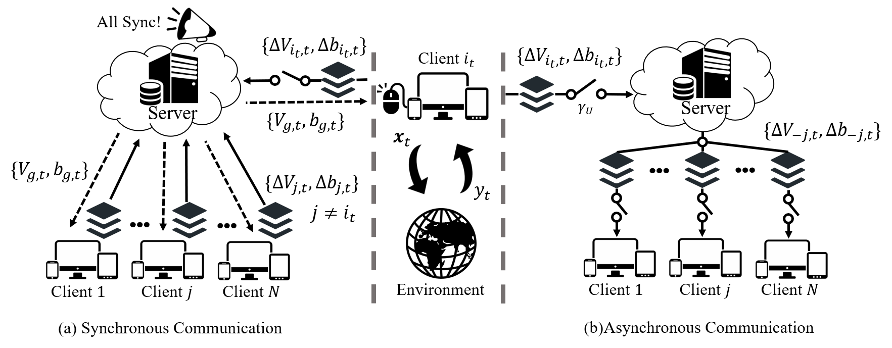
Figure 1: Comparison between the synchronous and asynchronous event-triggered communications for federated linear bandit. The former requires all clients to upload their latest data at once and then download the aggregated data, while latter performs both upload and download on a per-client basis.

Denote the set of time steps when client $i$ interacts with the environment up to time $t$ as $\mathcal{N}_{i}(t)=\left\{1\leq\tau\leq t:i_{\tau}=i\right\}$. Note that we do not impose any further assumption on the clients’ distribution or frequency of its interactions. This makes our setting more general than existing works (Wang et al., 2019; Dubey and Pentland, 2020), where the clients interact with the environment in a round-robin fashion, i.e., $|\mathcal{N}_{i}(t)|=t/N$. In addition, in the federated learning setting, the clients cannot directly communicate with each other, but can only communicate with the central server, i.e., a star-shaped communication network. Raw data collected by each client $\{(\mathbf{x}_{\tau},y_{\tau})\}_{\tau\in\mathcal{N}_{i}(t)}$ is stored locally and will not be transferred. Instead, the clients can only collaborate by communicating the parameters of the learning algorithm, e.g., gradients or sufficient statistics; and the communication cost is measured by the amount of parameters transferred across the system up to time $T$, which is denoted by $C_{T}$.

We consider two different settings about the linear reward mapping function $f_{i}(\cdot)$ for $i=1,\dots,N$:

Homogeneous clients.

Rewards received by all the clients are generated by a common reward mapping function:

$$f_{i}(\mathbf{x})=\theta^{\top}\mathbf{x},\quad\forall i\in[N]$$ (1)

where $\theta\in\mathbb{R}^{d}$ is the unknown parameter and we assume $\lVert\theta\rVert\leq 1$ and $\lVert\mathbf{x}\rVert\leq 1$. Despite its simplicity, this setting is commonly adopted in existing works for federated bandits.

Heterogeneous clients.

The unknown parameter for each client $i\in[N]$ consists of a globally shared component $\theta^{(g)}\in\mathbb{R}^{d_{g}}$ and a unique local component $\theta^{(i)}\in\mathbb{R}^{d_{i}}$:

$$f_{i}(\mathbf{x})=\begin{bmatrix}\theta^{(g)}\\ \theta^{(i)}\end{bmatrix}^{\top}\begin{bmatrix}\mathbf{x}^{(g)}\\ \mathbf{x}^{(l)}\end{bmatrix},\quad\forall i\in[N]$$ (2)

where $\mathbf{x}^{(g)}\in\mathbb{R}^{d_{g}}$, $\mathbf{x}^{(l)}\in\mathbb{R}^{d_{i}}$ denote the global and local features in $\mathbf{x}$, and we assume $||\theta^{(g)}||_{2}\leq 1$, $||\theta^{(i)}||_{2}\leq 1,\forall i\in[N]$ and $||\mathbf{x}^{(g)}||_{2}\leq 1$, $||\mathbf{x}^{(l)}||_{2}\leq 1$. This setting is more general and fits a larger variety of problems in practice. For example, $\mathbf{x}^{(g)}$ could be common arm features relevant to all the clients and $\mathbf{x}^{(l)}$ are those unique to client $i$. And our setting is flexible enough to allow different clients to have varying dimensions of their local features (i.e., $d_{i}\neq d_{j}$). Alternatively, when $\mathbf{x}^{(g)}\equiv\mathbf{x}^{(l)}$, this recovers the multi-task learning setting in Evgeniou and Pontil (2004).

We adopt the context regularity assumption from Gentile et al. (2014); Li et al. (2019a, 2021), which imposes a variance condition on the stochastic process generating $\mathbf{x}_{t,a}$ (for heterogeneous clients, it is imposed on global features $\mathbf{x}_{t,a}^{(g)}$). This suggests the informativeness of each observation in expectation.

Assumption 1 (Context regularity)

At each time $t$, the context vector $\mathbf{x}_{t,a}\in\mathcal{A}_{t}$ for each arm $a\in[K]$ is independently generated from a random process, such that

$$\mathbb{E}_{t-1}[\mathbf{x}_{t,a}\mathbf{x}_{t,a}^{\top}]:=\mathbb{E}[\mathbf{x}_{t,a}\mathbf{x}_{t,a}^{\top}|\{i_{s},\mathcal{A}_{s},\eta_{s}\}_{s\in[t-1]}]=\Sigma_{c}\succeq\lambda_{c}I,\forall t\in[T]$$

where the constant $\lambda_{c}>0$. Let also, for any fixed unit vector $z\in\mathbb{R}^{d}$, the random variable $(z^{\top}\mathbf{x}_{t,a})^{2}$ be conditionally sub-Gaussian with variance parameter $v^{2}\leq{\lambda_{c}^{2}}/{(8\log{4K})}$.

3.2 Asynchronous Communication Framework

In order to balance the two conflicting objectives, i.e., regret $R_{T}$ and communication cost $C_{T}$, we introduce an asynchronous event-triggered communication framework as illustrated in Figure 1(b). For simplicity, all discussions in this section assume homogeneous clients (Eq (1)), and we show in Section 3.4 that the result extends to heterogeneous clients (Eq (2)) as well with minor modifications. Also note that in this paper we use LinUCB (Abbasi-Yadkori et al., 2011) with our communication framework as a running example, but our results readily hold for other popular algorithms like LinTS (Abeille and Lazaric, 2017) and LinPHE (Kveton et al., 2019) .

We begin our discussion with an important observation about the instantaneous regret of linear bandit algorithms. Denote the sufficient statistics (for $\theta$) collected from all clients by time $t$ as ${V}_{t}=\sum_{\tau=1}^{t}\mathbf{x}_{\tau}\mathbf{x}_{\tau}^{\top}$ and ${b}_{t}=\sum_{\tau=1}^{t}\mathbf{x}_{\tau}y_{\tau}$. In a centralized setting, at each time step $t\in[T]$, $\{{V}_{t-1},{b}_{t-1}\}$ are readily available to make an informed choice of arm $\mathbf{x}_{t}\in\mathcal{A}_{t}$. It is known that the instantaneous regret $r_{t}$ incurred by the mentioned linear bandit algorithms is directly related to the width of the confidence ellipsoid in the direction of $\mathbf{x}_{t}$. Specifically, from Theorem 3 in (Abbasi-Yadkori et al., 2011), with probability at least $1-\delta$, the instantaneous regret $r_{t}$ incurred by LinUCB can be upper bounded by $r_{t}\leq 2\alpha_{t-1}\sqrt{\mathbf{x}_{t}^{\top}V_{t-1}^{-1}\mathbf{x}_{t}}$, where $\alpha_{t-1}=O\left(\sqrt{d\log{\frac{T}{\delta}}}\right)$. However, as data is decentralized in our problem, $\{{V}_{t-1},{b}_{t-1}\}$ are not readily available to client $i_{t}$. Instead, the client only has a delayed copy, denoted by $\{{V}_{i_{t},t-1},{b}_{i_{t},t-1}\}$, which is obtained by its own interactions with the environment on top of the last communication with the server. Therefore, now the instantaneous regret $r_{t}\leq 2\alpha_{i_{t},t-1}\sqrt{\mathbf{x}_{t}^{\top}V_{i_{t},t-1}^{-1}\mathbf{x}_{t}}=2\alpha_{i_{t},t-1}\sqrt{\mathbf{x}_{t}^{\top}{V}_{t-1}^{-1}\mathbf{x}_{t}}\sqrt{\Gamma_{t-1}}$, where $\Gamma_{t-1}=\frac{\mathbf{x}_{t}^{\top}{V}_{i_{t},t-1}^{-1}\mathbf{x}_{t}}{\mathbf{x}_{t}^{\top}{V}_{t-1}^{-1}\mathbf{x}_{t}}$ measures how much wider the confidence ellipsoid at client $i_{t}$’s estimation in the direction of $\mathbf{x}_{t}$ is, compared with that under a centralized setting. The value of $\Gamma_{t-1}$ depends on how frequent local updates are aggregated and shared via the server. Also note that $\Gamma_{t-1}\geq 1$, as ${V}_{t-1}\succeq{V}_{i_{t},t-1},\forall t$, which suggests the regret in the decentralized setting is at best the same as that in the centralized setting. Equality is attained when all the clients are synchronized in every time step.

Based on this observation, we can balance regret and communication cost by controlling the value of $\Gamma_{t-1}$. However, in the decentralized setting, neither the server nor the clients has direct access to $\{V_{t-1},b_{t-1}\}$, and the closest thing one can get is the aggregated sufficient statistics managed by the server, which we denote as $\{V_{g,t-1},b_{g,t-1}\}$. Hence, we take an indirect approach by first ensuring $\{V_{g,t-1},b_{g,t-1}\}$ do not deviate too much from $\{V_{t-1},b_{t-1}\}$, and then $\{V_{i,t-1},b_{i,t-1}\}$ do not deviate too much from $\{V_{g,t-1},b_{g,t-1}\}$ for each client $i\in[N]$. The former leads to the ‘upload’ event, i.e., each client decides whether to upload independently, and the latter leads to the ‘download’ event, i.e., the server decides whether to send its latest statistics to each client independently as well.

In the proposed communication framework shown in Figure 1(b), each client $i\in[N]$ stores a local copy of its sufficient statistics $\{V_{i,t-1},b_{i,t-1}\}$, and also an ‘upload’ buffer $\{\Delta V_{i,t-1},\Delta b_{i,t-1}\}$, i.e., client $i$’s local updates that have not been sent to the server. At each time step $t$, client $i_{t}\in[N]$ interacts with the environment, and updates $V_{i_{t},t}=V_{i_{t},t-1}+\mathbf{x}_{t}\mathbf{x}_{t}^{\top},b_{i_{t},t}=b_{i_{t},t-1}+\mathbf{x}_{t}y_{t}$, $\Delta V_{i_{t},t}=\Delta V_{i_{t},t-1}+\mathbf{x}_{t}\mathbf{x}_{t}^{\top},\Delta b_{i_{t},t}=\Delta b_{i_{t},t-1}+\mathbf{x}_{t}y_{t}$ with the new observation $(\mathbf{x}_{t},y_{t})$. Then it starts executing Algorithm 1, by first checking the following condition (line 2):

‘Upload’ event: Client $i_{t}$ sends $\{\Delta V_{i_{t},t},\Delta b_{i_{t},t}\}$ to the server if event:

$$\mathcal{U}_{t}(\gamma_{U})=\left\{\frac{\det(V_{i_{t},t})}{\det(V_{i_{t},t}-\Delta V_{i_{t},t})}>\gamma_{U}\right\}$$ (3)

happens, and then sets $\Delta V_{i,t}=\textbf{0},\Delta b_{i,t}=\textbf{0}$. Otherwise, $\{\Delta V_{i,t},\Delta b_{i,t}\}$ remain unchanged.

The server stores the aggregated sufficient statistics $\{V_{g,t-1},b_{g,t-1}\}$ over the local updates received from the clients, and also maintains ‘download’ buffers $\{\Delta V_{-j,t-1},\Delta b_{-j,t-1}\}$ for each client $j\in[N]$, i.e., the aggregated updates that have not been sent to client $j$. Specifically, after the server receives $\{\Delta V_{i_{t},t},\Delta b_{i_{t},t}\}$ via the ‘upload’ from client $i_{t}$, it updates $V_{g,t}=V_{g,t-1}+\Delta V_{i_{t},t},b_{g,t}=b_{g,t-1}+\Delta b_{i_{t},t}$, and $\Delta V_{-j,t}=\Delta V_{-j,t-1}+\Delta V_{i_{t},t},\Delta b_{-j,t}=\Delta b_{-j,t-1}+\Delta b_{i_{t},t}$ for all clients $j\neq i_{t}$. Then it checks the following condition for each client $j\neq i_{t}$ (line 7):

‘Download’ event: The server sends $\{\Delta V_{j,t},\Delta b_{j,t}\}$ to client $j$ if event:

$$\mathcal{D}_{t,j}(\gamma_{D})=\left\{\frac{\det(V_{g.t})}{\det(V_{g,t}-\Delta V_{-j,t})}>\gamma_{D}\right\}$$ (4)

happens, and then sets $\Delta V_{-j,t}=\textbf{0},\Delta b_{-j,t}=\textbf{0}$. Otherwise, $\{\Delta V_{-j,t},\Delta b_{-j,t}\}$ remain unchanged.

After client $j$ receives $\{\Delta V_{-j,t},\Delta b_{-j,t}\}$ via the ‘download’ communication, it updates $V_{j,t}=V_{j,t-1}+\Delta V_{-j,t},b_{j,t}=b_{j,t-1}+\Delta b_{-j,t}$.

Algorithm 1 Event-triggered Communication Protocol

1:  Input: thresholds $\gamma_{U},\gamma_{D}\geq 1$

2:  if  Event $\mathcal{U}_{t}(\gamma_{U})$ in Eq (3) happens then

3:     Upload $\Delta{V}_{i_{t},t},\Delta{b}_{i_{t},t}$ ($\text{client }i_{t}\rightarrow\text{server}$)

4:     Update server: $V_{g,t}\mathrel{+}=\Delta V_{i_{t},t},b_{g,t}\mathrel{+}=\Delta b_{i_{t},t}$, $\Delta V_{-j,t}\mathrel{+}=\Delta V_{i_{t},t},\Delta b_{-j,t}\mathrel{+}=\Delta b_{i_{t},t}$, $\forall j\neq i_{t}$

5:     Client $i_{t}$ sets $\Delta{V}_{i_{t},t}=\textbf{0}$, $\Delta{b}_{i_{t},t}=\textbf{0}$

6:     for $j=1,\dots,N$ do

7:        if  Event $\mathcal{D}_{t,j}(\gamma_{D})$ in Eq (4) happens then

8:           Download $\Delta{V}_{-j,t},\Delta{b}_{-j,t}$ ($\text{server}\rightarrow\text{client }j$)

9:           Update client $j$: $V_{j,t}\mathrel{+}=\Delta V_{-j,t},b_{j,t}\mathrel{+}=\Delta b_{-j,t}$

10:           Server sets $\Delta{V}_{-j,t}=\textbf{0},\Delta{b}_{-j,t}=\textbf{0}$

11:        end if

12:     end for

13:  end if

The following lemma specifies an upper bound of $\Gamma_{t-1}$ by executing Algorithm 1, which depends on the thresholds $\{\gamma_{U},\gamma_{D}\}$ and the number of clients $N$.

Lemma 1

Under Assumption 1, the ‘upload’ and ‘download’ triggering events defined in Eq (3) and Eq (4), then w.h.p. $\Gamma_{t-1}\leq\frac{8\gamma_{D}}{\lambda_{c}}[1+(N-1)(\gamma_{U}-1)],\forall t$.

Proof of Lemma 1 is given in appendix. The main idea is to use $\det(V_{g,t-1})$ as an intermediate between $\det(V_{i_{t},t-1})$ and $\det(V_{t-1})$, which are separately controlled by the ‘download’ and ‘upload’ events. When setting $\gamma_{D}=\gamma_{U}=1$, $\Gamma_{t-1}=1$, $\forall t\in[T]$, which means global synchronization happens at each time step, it recovers the regret incurred in the centralized setting.

Synchronous vs. asynchronous communication: As shown in Figure 1(a), in the synchronous protocol (Appendix G in (Wang et al., 2019)), when a synchronization round is triggered by a client $i_{t}$, the server asks all the clients to upload their local updates (illustrated as solid lines), aggregates them, and then sends the aggregated update back (illustrated as dashed lines). This ‘two-way’ communication is vulnerable to delays or unavailability of clients, which are common in a distributed setting. In comparison, our asynchronous communication, as shown in Figure 1(b), is more robust because the server only concerns the clients whose ‘download’ condition has been met, which does not need other clients’ acknowledgement. In addition, when the clients have distinct availability of new observations, which is usually the case for most applications, synchronizing all $N$ clients leads to inefficient communication as some clients may have very few new observations since last synchronization. We will show later that this unfortunately leads to an increased rate in $N$ in the upper bound of $C_{T}$, compared with our asynchronous communication.

Multiple clients per time: Note that essentially both Algorithm 1 and the synchronous protocol assumed only one active client per time, i.e., the communication protocol is executed after the current client receives a new observation and completed before the next client shows up. This setup simplifies the description and also makes the theoretical results compatible with standard linear bandit setting. Otherwise, we will need to introduce additional assumptions to quantify the extent of delay in the communication for regret analysis. In reality, each client is an independent process interacting with its environment, e.g., serving its user population, so that there could be many active clients at the same time. In the proposed asynchronous protocol, when a client triggers the upload event, it will immediately send the data in its buffer to the server; the server, upon receiving the uploaded data from any client, will immediately aggregate this data and check the download events to see which client needs a download. Thus, different from the synchronous protocol where the server ensures all the clients have the same model after each download, we allow both the server and the clients to update their model at any time without the need of any global synchronization.

3.3 Learning with Homogeneous Clients

Based on the asynchronous event-triggered communication, we design the Asynchronous LinUCB Algorithm (Async-LinUCB) for homogeneous clients. Detailed steps are explained in Algorithm 2.

Arm selection: At each time step $t=1,\dots,T$, client $i_{t}$ selects an arm $\mathbf{x}_{t}\in\mathcal{A}_{t}$ using the the UCB strategy. Specifically, client $i_{t}$ pulls arm $\mathbf{x}_{t}$ that maximizes the UCB score computed as follows (line 8),

$$\mathbf{x}_{t}=\operatorname*{arg\,max}_{\mathbf{x}\in\mathcal{A}_{t}}{\mathbf{x}^{\top}\hat{\theta}_{i_{t},t-1}(\lambda)+\text{CB}_{i_{t},t-1}(\mathbf{x})}$$ (5)

where $\hat{\theta}_{i_{t},t-1}(\lambda)=V_{i_{t},t-1}(\lambda)^{-1}b_{i_{t},t-1}$ is the ridge regression estimator with regularization parameter $\lambda$; $V_{i_{t},t-1}(\lambda)=V_{i_{t},t-1}+\lambda I$; and the confidence bound of reward estimation for arm $\mathbf{x}$ is $\text{CB}_{i_{t},t-1}(\mathbf{x})=\alpha_{i_{t},t-1}||\mathbf{x}||_{V_{i_{t},t-1}(\lambda)^{-1}}$, where $\alpha_{i_{t},t-1}=\sigma\sqrt{\log{\frac{\det{V_{i_{t},t-1}(\lambda)}}{\det{\lambda I}}}+2\log{1/\delta}}+\sqrt{\lambda}$. After client $i_{t}$ observes reward $y_{t}$ and updates locally (line 9), it proceeds with the asynchronous event-triggered communication (line 10), and sends updates accordingly.

Algorithm 2 Async-LinUCB

1:  Input: thresholds $\gamma_{U},\gamma_{D}\geq 1$, $\sigma,\lambda>0$, $\delta\in(0,1)$

2:  Initialize server: ${V}_{g,0}=\textbf{0}_{d,d}$, ${b}_{g,0}=\textbf{0}_{d}$

3:  for  $t=1,2,...,T$ do

4:     Observe arm set $\mathcal{A}_{t}$ for client $i_{t}\in[N]$

5:     if client $i_{t}$ is new then

6:        Initialize client $i_{t}$: ${V}_{i_{t},t-1}=\textbf{0}_{d,d}$, ${b}_{i_{t},t-1}=\textbf{0}_{d}$, $\Delta{V}_{i_{t},t-1}=\textbf{0}_{d,d}$, $\Delta{b}_{i_{t},t-1}=\textbf{0}_{d}$

7:        Initialize server’s download buffer for client $i_{t}$: $\Delta{V}_{-i_{t},t-1}=V_{g,t-1}$, $\Delta{b}_{-i_{t},t-1}=b_{g,t-1}$

8:     end if

9:     Select arm $\mathbf{x}_{t}\in\mathcal{A}_{t}$ by Eq (5) and observe reward $y_{t}$

10:     Update client $i_{t}$: ${V}_{i_{t},t}\mathrel{+}=\mathbf{x}_{t}\mathbf{x}_{t}^{T}$, ${b}_{i_{t},t}\mathrel{+}=\mathbf{x}_{t}y_{t}$, $\Delta{V}_{i_{t},t}\mathrel{+}=\mathbf{x}_{t}\mathbf{x}_{t}^{T}$, $\Delta{b}_{i_{t},t}+=\mathbf{x}_{t}y_{t}$

11:     Event-triggered Communications (Algorithm 1)

12:  end for

The upper bounds of cumulative regret $R_{T}$ and communication cost $C_{T}$ incurred by Async-LinUCB are given in Theorem 2 (proof provided in appendix). Note that as discussed in Section 3.2, clients collaborate by transferring updates of the sufficient statistics, i.e., $\{\Delta V\in\mathbb{R}^{d\times d},\Delta b\in\mathbb{R}^{d}\}$. Since our target is not to reduce the size of these parameters, we define the communication cost $C_{T}$ as the number of times $\{\Delta V,\Delta b\}$ being transferred between agents.

Theorem 2 (Regret and Communication Cost)

With Assumption 1, and the communication thresholds $\gamma_{U},\gamma_{D}$, then w.h.p., the cumulative regret

$$R_{T}=O\left(d\sqrt{T\log^{2}{T}}\min(\sqrt{N},\sqrt{\gamma_{D}[1+(N-1)(\gamma_{U}-1)]})\right)$$

and communication

$$C_{T}=O\bigl{(}dN{\log{T}}/{\log{\min{(\gamma_{U},\gamma_{D})}}}\bigr{)}$$

The thresholds $\gamma_{U},\gamma_{D}$ can be flexibly adjusted to trade-off between $R_{T}$ and $C_{T}$, e.g., interpolate between the two extreme cases: clients never communicate ($R_{T}=O(N^{1/2}d\sqrt{T}\log{T})$); and clients are synchronized in every time step ($R_{T}=O(d\sqrt{T}\log{T})$). Details about threshold selection and the corresponding theoretical results are provided in appendix. For simplicity, we fix $\gamma_{U}=\gamma_{D}=\gamma$ in the following discussions, but one can choose different values to have a finer control especially for applications where the cost of upload and download communication differs. Based on Theorem 2, to attain $R_{T}=O(N^{1/4}d\sqrt{T}\log{T})$, Async-LinUCB needs $C_{T}=O(N^{3/2}d\log{T})$ (by setting $\gamma=\exp(N^{-\frac{1}{2}})$). To attain the same $R_{T}$, the corresponding $C_{T}$ of Sync-LinUCB is smaller than ours by a factor of $O(N^{1/4})$ only under uniform client distribution ($P(i_{t}=i)=\frac{1}{N},\forall i\in[N]$), while under non-uniform client distribution, which is almost always the case in practice, it is higher than ours by a factor of $O(N^{1/4})$. The description and theoretical analysis of Sync-LinUCB under uniform and non-uniform client distribution are given in appendix.

3.4 Learning with Heterogeneous Clients

In this section, we study the setting of heterogeneous clients as defined in Eq (2). As the clients only share $\theta^{(g)}$, we need to learn the global component $\theta^{(g)}$ collaboratively by all clients, while learning the personalized local component $\theta^{(i)}$ individually for each client $i$. We adopt an Alternating Minimization (AM) method to separately update the two components, and use the asynchronous communication framework in Algorithm 1 to ensure communication-efficient learning of $\theta^{(g)}$. The resulting algorithm is named Asynchronous LinUCB with Alternating Minimization (Async-LinUCB-AM), and its detailed steps are given in Algorithm 3 .

Algorithm 3 Async-LinUCB-AM

1:  Input: thresholds $\gamma_{U},\gamma_{D}\geq 1$, $\sigma,\lambda>0$, $\delta\in(0,1)$

2:  Initialize server: ${V}_{g,0}=\textbf{0}_{d_{g}\times d_{g}}$, ${b}_{g,0}=\textbf{0}_{d_{g}}$

3:  for  $t=1,2,...,T$ do

4:     Observe arm set $\mathcal{A}_{t}$ for client $i_{t}\in[N]$

5:     if Client $i_{t}$ is new then

6:        Initialize client $i_{t}$: ${V}_{i_{t},t-1}=\textbf{0}_{d_{g}\times d_{g}}$, ${b}_{i_{t},t-1}=\textbf{0}_{d_{g}}$, $\Delta{V}_{i_{t},t-1}=\textbf{0}_{d_{g}\times d_{g}}$, $\Delta{b}_{i_{t},t-1}=\textbf{0}_{d_{g}}$, ${V}^{(l)}_{i_{t},t-1}=\textbf{0}_{d_{i_{t}},d_{i_{t}}}$, ${b}^{(l)}_{i_{t},t-1}=\textbf{0}_{d_{i_{t}}}$

7:        Initialize server’s download buffer for client $i_{t}$: $\Delta{V}_{-i_{t},t-1}=V_{g,t-1}$, $\Delta{b}_{-i_{t},t-1}=b_{g,t-1}$

8:     end if

9:     Select arm $\mathbf{x}_{t}\in\mathcal{A}_{t}$ by Eq (8) and observe reward $y_{t}$

10:     Run AM by Eq (7) to estimate partial rewards: $\hat{y}^{(g)}_{t}=y_{t}-{\mathbf{x}_{t}^{(l)}}^{\top}\hat{\theta}^{(l)}_{i_{t},t}$, $\hat{y}^{(l)}_{t}=y_{t}-{\mathbf{x}_{t}^{(g)}}^{\top}\hat{\theta}^{(g)}_{i_{t},t}$

11:     Update client $i_{t}$: ${V}_{i_{t},t}\mathrel{+}=\mathbf{x}_{t}^{(g)}{\mathbf{x}_{t}^{(g)}}^{\top}$, ${b}_{i_{t},t}\mathrel{+}=\mathbf{x}^{(g)}_{t}\hat{y}^{(g)}_{t}$, $\Delta{V}_{i_{t},t}\mathrel{+}=\mathbf{x}_{t}^{(g)}{\mathbf{x}_{t}^{(g)}}^{\top}$, $\Delta{b}_{i_{t},t}+=\mathbf{x}^{(g)}_{t}\hat{y}^{(g)}_{t}$, ${V}^{(l)}_{i_{t},t}\mathrel{+}=\mathbf{x}_{t}^{(l)}{\mathbf{x}_{t}^{(l)}}^{\top}$, ${b}^{(l)}_{i_{t},t}\mathrel{+}=\mathbf{x}^{(l)}_{t}\hat{y}^{(l)}_{t}$

12:     Event-triggered Communications (Algorithm 1)

13:  end for

Alternating Minimization: In a centralized learning setting, applying AM to iteratively update the estimation of the local component and global component is straightforward:

$$\begin{split}&\hat{\theta}^{(l)}_{i,t}=\textit{proj}_{\mathbb{B}_{2}^{d_{i}}(1)}\bigl{(}({V}^{(l)}_{i,t})^{-}{b}^{(l)}_{i,t}\bigr{)},\forall i\in[N]\\ &\hat{\theta}^{(g)}_{t}=\textit{proj}_{\mathbb{B}_{2}^{d_{g}}(1)}\bigl{(}({V}_{t})^{-}{b}_{t}\bigr{)}\end{split}$$ (6)

where $\mathbb{B}_{2}^{d}(1)=\{\theta\in\mathbb{R}^{d}:||\theta||_{2}\leq 1\}$ denotes the unit $\ell_{2}$ ball, $(\cdot)^{-}$ denotes generalized matrix inverse, $\textit{proj}_{\Theta}(\cdot)$ denotes the Euclidean projection onto $L_{2}$ ball $\Theta$, ${V}^{(l)}_{i,t}=\sum_{\tau\in\mathcal{N}_{i}(t)}\mathbf{x}_{\tau}^{(l)}{\mathbf{x}_{\tau}^{(l)}}^{\top}$, ${b}^{(l)}_{i,t}=\sum_{\tau\in\mathcal{N}_{i}(t)}\mathbf{x}_{\tau}^{(l)}(y_{\tau}-{\mathbf{x}_{\tau}^{(g)}}^{\top}\hat{\theta}_{t}^{(g)})$, ${V}_{t}=\sum_{\tau=1}^{t}\mathbf{x}_{\tau}^{(g)}{\mathbf{x}_{\tau}^{(g)}}^{\top}$, and ${b}_{t}=\sum_{\tau=1}^{t}\mathbf{x}_{\tau}^{(g)}(y_{\tau}-{\mathbf{x}_{\tau}^{(l)}}^{\top}\hat{\theta}^{(l)}_{i_{\tau},t})$.

However, iteratively executing Eq (6) is impractical under federated setting: first, $\{{V}_{t},{b}_{t}\}$ are distributed across the clients; second, iteratively updating $b_{t}$ and $b^{(l)}_{i,t}$ requires storage of raw history data. This incurs space and communication complexities that are linear in time $T$. Instead, we modify Eq (6) to get the following update rule. At time $t$, after client $i_{t}$ obtains a new data point $(\mathbf{x}_{t},y_{t})$ from the environment, it alternates between the following two steps (line 9):

$$\begin{split}\hat{\theta}^{(l)}_{i_{t},t}&=\textit{proj}_{\mathbb{B}_{2}^{d_{i}}(1)}\left(({V}^{(l)}_{i_{t},t-1}+\mathbf{x}_{t}^{(l)}{\mathbf{x}_{t}^{(l)}}^{\top})^{-}({b}^{(l)}_{i_{t},t-1}+\mathbf{x}_{t}^{(l)}\hat{y}^{(l)}_{t})\right)\\ \hat{\theta}^{(g)}_{i_{t},t}&=\textit{proj}_{\mathbb{B}_{2}^{d_{g}}(1)}\left((V_{i_{t},t-1}+\mathbf{x}_{t}^{(g)}{\mathbf{x}_{t}^{(g)}}^{\top})^{-}({b}_{i_{t},t-1}+\mathbf{x}_{t}^{(g)}\hat{y}^{(g)}_{t})\right)\end{split}$$ (7)

where $\hat{y}^{(l)}_{t}=y_{t}-{\mathbf{x}_{t}^{(g)}}^{\top}\hat{\theta}^{(g)}_{i_{t},t}$ and $\hat{y}^{(g)}_{t}=y_{t}-{\mathbf{x}_{t}^{(l)}}^{\top}\hat{\theta}^{(l)}_{i_{t},t}$ denote the estimated ‘partial’ rewards for $\theta^{(i)}$ and $\theta^{(g)}$, and $\{{V}_{i,t-1},{b}_{i,t-1}\}$ denote client $i$’s local copy of the sufficient statistics for $\theta^{(g)}$. Then $\hat{y}^{(g)}_{t}$ and $\hat{y}^{(l)}_{t}$ are used to locally update the sufficient statistics of client $i_{t}$ (line 10 in Algorithm 3). Compared with Eq (6) that iteratively updates the estimated ‘partial’ rewards on all historic data from different clients, Eq (7) only updates that on $(\mathbf{x}_{t},y_{t})$ while keeping the rest fixed. This incurs constant space complexity and no communication cost. Though this comes at a price of slower convergence on the estimators, we later prove that this will not sacrifice the accumulative regret too much.

Since the local component is unique to each client, only $\{{V}_{i,t-1},{b}_{i,t-1}\}$ for estimating the global component need to be shared among clients. Our asynchronous communication protocol can be directly applied here (line 11) to ensure communication efficiency.

Arm selection: Client $i_{t}$ selects arm $\mathbf{x}_{t}\in\mathcal{A}_{t}$ via the UCB strategy (line 8 in Algorithm 3). Confidence ellipsoids for the estimations obtained by Eq (7) are given in Lemma 3. Now the UCB score consists of two terms corresponding to the global and local component estimations, respectively:

$$\mathbf{x}_{t}=\operatorname*{arg\,max}_{\mathbf{x}\in\mathcal{A}_{t}}{\text{UCB}^{(g)}_{i_{t},t-1}({\mathbf{x}^{(g)}})+\text{UCB}^{(l)}_{i_{t},t-1}({\mathbf{x}^{(l)}})}$$ (8)

where $\text{UCB}^{(g)}_{i_{t},t-1}({\mathbf{x}^{(g)}})={\mathbf{x}^{(g)}}^{\top}\hat{\theta}^{(g)}_{i_{t},t-1}(\lambda)+\alpha^{(g)}_{i_{t},t-1}||\mathbf{x}^{(g)}||_{V_{i_{t},t-1}(\lambda)^{-1}}$, $\text{UCB}^{(l)}_{i_{t},t-1}({\mathbf{x}^{(l)}})={\mathbf{x}^{(l)}}^{\top}\hat{\theta}^{(l)}_{i_{t},t-1}(\lambda)+\alpha^{(l)}_{i_{t},t-1}||\mathbf{x}^{(l)}||_{V^{(l)}_{i_{t},t-1}(\lambda)^{-1}}$. $\hat{\theta}^{(g)}_{i_{t},t-1}(\lambda)=V_{i_{t},t-1}(\lambda)^{-1}b_{i_{t},t-1}$ is the ridge regression estimator for the global component with the regularization parameter $\lambda$. $\hat{\theta}^{(l)}_{i_{t},t-1}(\lambda)=V^{(l)}_{i_{t},t-1}(\lambda)^{-1}b^{(l)}_{i_{t},t-1}$ is the ridge regression estimator for the local component with the regularization parameter $\lambda$. $\alpha^{(g)}_{i_{t},t-1}$ and $\alpha^{(l)}_{i_{t},t-1}$ are given in Lemma 3 (proof given in appendix).

Lemma 3 (Confidence ellipsoids)

With probability at least $1-\delta$, $||\hat{\theta}^{(g)}_{i,t}(\lambda)-\theta^{(g)}||_{V_{i,t}(\lambda)}\leq\alpha^{(g)}_{i,t}$, where $\alpha^{(g)}_{i,t}=(\sigma+2)\sqrt{\log{\frac{\det{V_{i,t}(\lambda)}}{\det{\lambda I}}}+2\log{1/\delta}}+\sqrt{\lambda}$. And with probability at least $1-\delta$, $||\hat{\theta}^{(l)}_{i,t}(\lambda)-\theta^{(i)}||_{V^{(l)}_{i,t}(\lambda)}\leq\alpha^{(l)}_{i,t}$, where $\alpha^{(l)}_{i,t}=(\sigma+2)\sqrt{\log{\frac{\det{V^{(l)}_{i,t}(\lambda)}}{\det{\lambda I}}+2\log{1/\delta}}}+\sqrt{\lambda}$.

Then based on the constructed confidence ellipsoid, we can prove Theorem 4 (proof given in appendix), which provides the upper bounds of cumulative regret $R_{T}$ and communication cost $C_{T}$ incurred by Async-LinUCB-AM.

Theorem 4 (Regret and Communication Cost)

With Assumption 1, and the communication thresholds $\gamma_{U},\gamma_{D}$, then w.h.p., the cumulative regret

$$R_{T}=O\bigl{(}d_{g}\sqrt{T\log^{2}{T}}\min(\sqrt{N},\sqrt{\gamma_{D}[1+(N-1)(\gamma_{U}-1)]}+\sum_{i=1}^{N}d_{i}\sqrt{|\mathcal{N}_{i}(T)|\log^{2}{|\mathcal{N}_{i}(T)|}}\bigr{)}$$

and communication cost

$$C_{T}=O(d_{g}N\log{T}/\log{\min(\gamma_{U},\gamma_{D})})$$

Note that the regret upper bound of Async-LinUCB-AM consists of two terms: the first term corresponds to the global components $\theta^{(g)}$, which enjoys the benefit of communication; and the second term corresponds to the unique local components $\theta^{(i)}$ of each client, which essentially matches the regret upper bound for running $N$ LinUCB independently for $\theta^{(i)}$ of each client. Intuitively, when the problems solved by different clients become more similar, then the first term dominates as $d_{g}$ becomes larger compared with $d_{i}$.

4 Experiments

We performed extensive empirical evaluations of Async-LinUCB and Async-LinUCB-AM on both synthetic and real-world datasets (we set $\gamma_{U}=\gamma_{D}=\gamma$ in all experiments), and included Sync-LinUCB (Wang et al., 2019) as baseline.

4.1 Experiments on Synthetic Dataset

To validate our theoretical analysis in Section 3.3 and Section 3.4, two sets of simulation experiments were conducted. We first conducted simulation experiment in homogeneous client setting to validate our theoretical comparison between Async-LinUCB and Sync-LinUCB (see Section 3.3 and Section E in appendix), i.e., how well the algorithms balance regret $R_{T}$ and communication cost $C_{T}$ under uniform and non-uniform client distributions. Then we conducted simulation experiment in heterogeneous setting to validate our regret upper bound for Async-LinUCB-AM (see Section 3.4), i.e., how the portion of global components $\frac{d_{g}}{d_{g}+d_{i}}$ in the bandit parameter affects the regret of Async-LinUCB-AM.

4.1.1 Synthetic dataset.

We simulated the federated linear bandit problem setting in Section 3.1, with $T=30000,N=1000$, and $\mathcal{A}_{t}$ ($K=25$) uniformly sampled from a $\ell_{2}$ ball. (1) Homogeneous clients: To compare how the algorithms balance $R_{T}$ and $C_{T}$ under uniform ($P(i_{t}=i)=\frac{1}{N},\forall i,t$) and non-uniform client distributions ($P(i_{t})$ is an arbitrary point on probability simplex), we fixed $d=25$, and ran Async-LinUCB and Sync-LinUCB with a large range of threshold values (logarithmically spaced between $10^{-2}$ and $10^{3}$). (2) Heterogeneous clients: To see how $R_{T}$ and $C_{T}$ of Async-LinUCB-AM changes as the portion of global components change, we set the local components for all clients to have equal dimension, i.e., $d_{i}=d_{l},\forall i\in[N]$, fixed $d_{g}+d_{l}=25$, $\forall i\in[N]$, and then ran Async-LinUCB-AM (with $\gamma=5$) under varying $d_{g}\in\{4,8,12,16,20,24\}$.

4.1.2 Experiment results.

Experiment results (averaged over $10$ runs) on synthetic dataset are shown in Figure 2(a)-2(c). Note that in the scatter plots, each dot denotes the cumulative communication cost (x-axis) and regret (y-axis) that an algorithm (Async-LinUCB or Sync-LinUCB) with certain threshold value (labeled next to the dot) has obtained at iteration $T$.

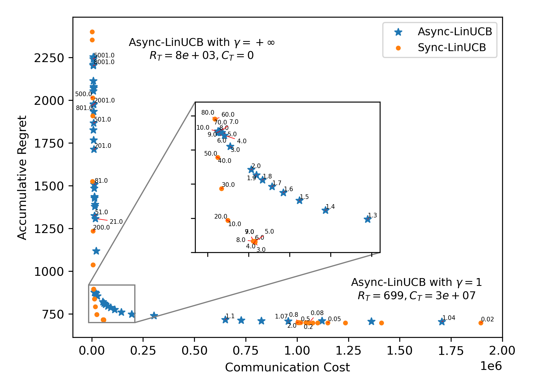
(a) Homogeneous (uniform client distribution)

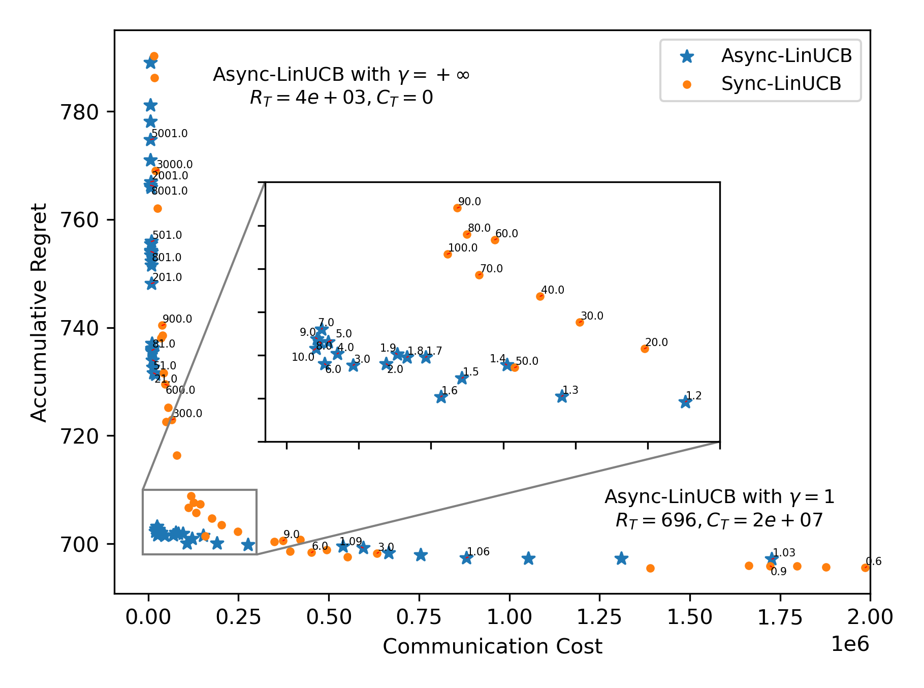
(b) Homogeneous (non-uniform client distribution)

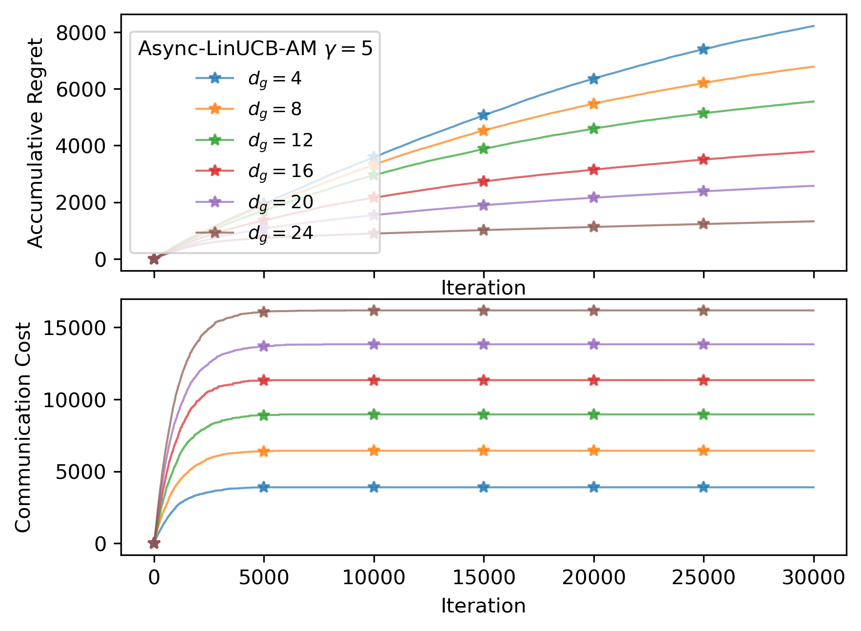
(c) Heterogeneous clients

Figure 2: Experiment results on synthetic dataset.

(1) Homogeneous clients (Figure 2(a)-2(b)): From both Figure 2(a) and Figure 2(b), we can see that as the threshold value increases, $C_{T}$ decreases and $R_{T}$ increases, and that the use of event-triggered communication significantly reduces $C_{T}$ while attaining low $R_{T}$, compared with synchronizing all the clients at each time step (Async-LinUCB with $\gamma=1$). In Figure 2(a), Sync-LinUCB has lower $C_{T}$ than Async-LinUCB under the same $R_{T}$, and in Figure 2(b), Async-LinUCB has lower $C_{T}$ than Sync-LinUCB under the same $R_{T}$, which conform with our theoretical results that Sync-LinUCB has inefficient communication under non-uniform client distribution.

(2) Heterogeneous clients (Figure 2(c)): By increasing the portion of global components $\theta^{g}$ in the bandit parameter, we can observe a clear trend in both regret and communication cost, i.e., the regret keeps decreasing while the communication cost keeps increasing. This validates our theoretical analysis about $R_{T}$ and $C_{T}$ in Section 3.4. With $d_{g}$ increases and $d_{l}$ decreases, the first term in the upper bound of $R_{T}$ dominates (which grows slower w.r.t. $N$ compared with the second term), leading to the decreased regret, but the communication cost would increase since $C_{T}=O(d_{g}N\log{T})$.

4.2 Experiments on Real-world Dataset

We continue investigating the effectiveness of our proposed solution on real-world datasets. Note that these real-world datasets do not necessarily satisfy the assumption that all the clients are homogeneous, in other words not all the users have the same preference, we pay special attention to Async-LinUCB-AM in the comparison, by setting $x_{g}\equiv x_{i},\forall i\in[N]$, as mentioned in Section 3.1. This allows the clients to learn a global model collaboratively, and in the meantime each learns a personalized model independently. Intuitively, this should make Async-LinUCB-AM more robust to different settings, i.e., the clients are either homogeneous or heterogeneous.

4.2.1 Real-world dataset.

We compared Async-LinUCB, Async-LinUCB-AM and Sync-LinUCB on three public recommendation datasets: LastFM, Delicious and MovieLens (Cantador et al., 2011; Harper and Konstan, 2015), with various threshold values (logarithmically spaced between $10^{-2}$ and $10^{3}$). The LastFM dataset contains $N=1892$ users, 17632 items (artists), and $T=96733$ interactions. We consider the “listened artists” in each user as positive feedback. The Delicious dataset contains $N=1861$ users, 69226 items (URLs), and $T=104799$ interactions. We treat the bookmarked URLs in each user as positive feedback. The MovieLens dataset used in the experiment is extracted from the MovieLens 20M dataset by keeping users with over $3000$ observations, which results in a dataset with $N=54$ users, 26567 items (movies), and $T=214729$ interactions. We consider all items with non-zero ratings as positive feedback. The datasets were preprocessed following the procedure in Cesa-Bianchi et al. (2013) to fit the linear bandit setting (with TF-IDF feature $d=25$ and arm set $K=25$).

4.2.2 Experiment results.

Experiment results on the three real-world datasets are shown in Figure 3(a)-3(c). In the scatter plots, each dot denotes the cumulative communication cost (x-axis) and normalized reward by a random strategy (y-axis) that an algorithm (Async-LinUCB, Async-LinUCB-AM, or Sync-LinUCB) with certain threshold value (labeled next to the dot) has obtained at iteration $T$. To understand the results of these algorithms on the three real-world datasets, we can first look at how well the two extreme cases, Async-LinUCB with $\gamma=1$ (as the communication cost of this algorithm is outside of the figure, its result is illustrated as text label) and Async-LinUCB with $\gamma=+\infty$ perform.

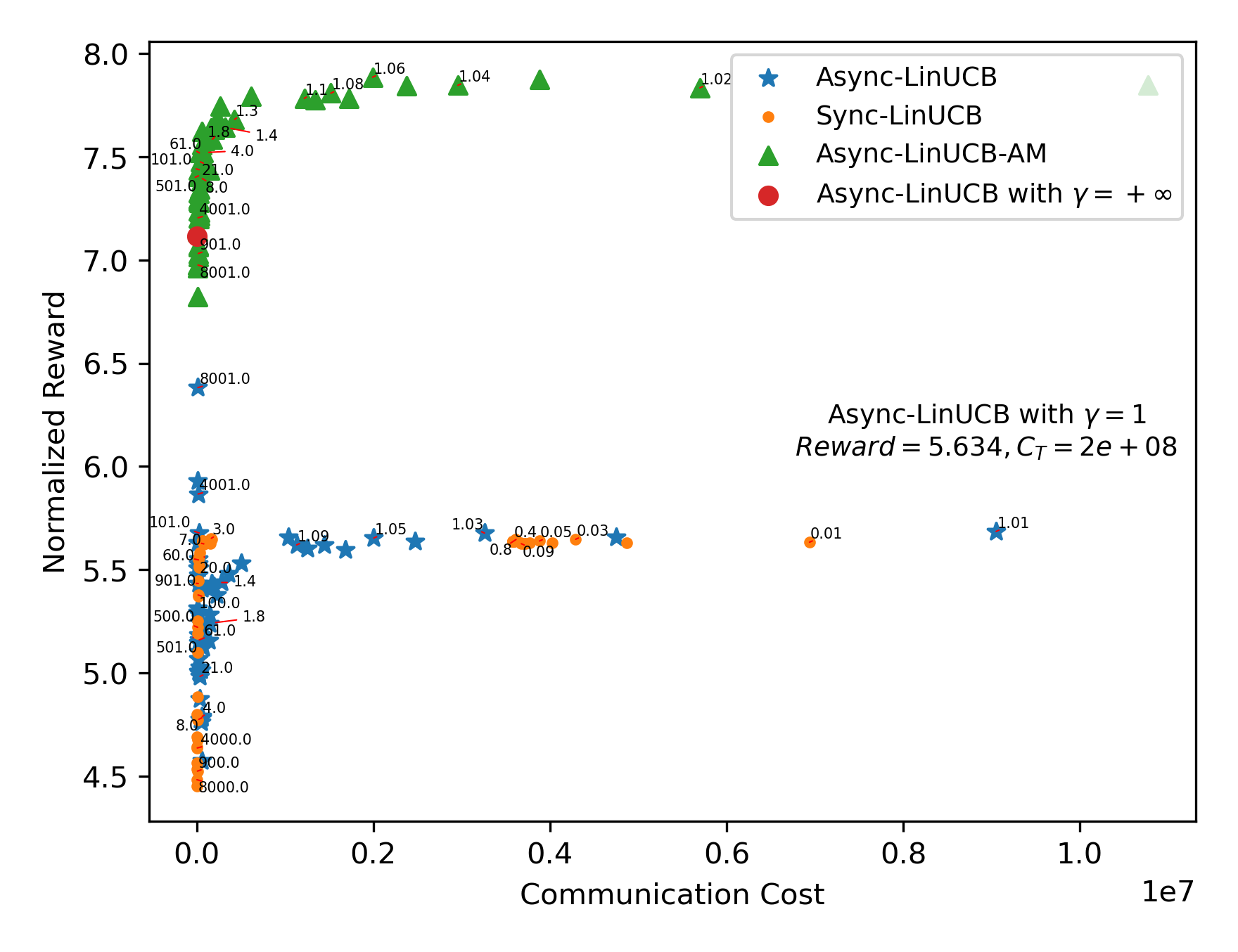
(a) LastFM ($N=1892$)

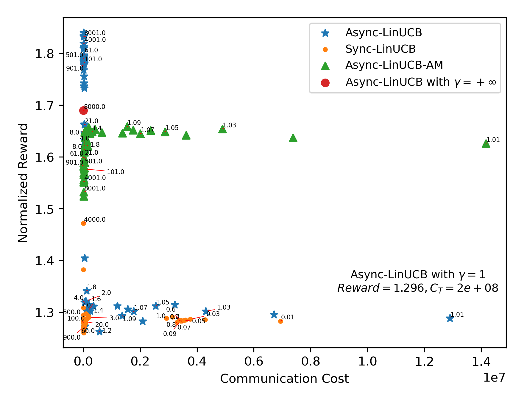
(b) Delicious ($N=1867$)

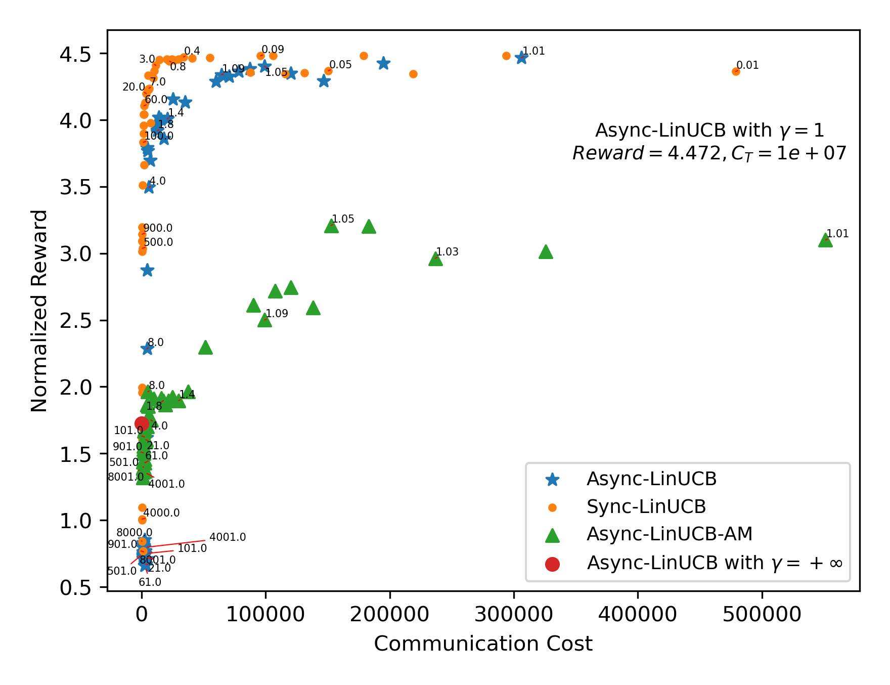
(c) MovieLens ($N=54$)

Figure 3: Experiment results on real-world recommendation datasets.

(1) LastFM & Delicious (Figure 3(a)-3(b)): On both LastFM and Delicious datasets, Async-LinUCB with $\gamma=+\infty$ (illustrated as the red dot) attains very high reward, which suggests users in these two datasets have very diverse preferences, such that aggregating their data has a negative impact on the performance. Since the homogeneous clients assumption does not hold in this case, both Async-LinUCB and Sync-LinUCB perform as badly as the extreme case of Async-LinUCB with $\gamma=1$, which is especially true when the clients frequently communicate with each other, i.e., with lower threshold values. In comparison, Async-LinUCB-AM attains relatively good performance even when the clients frequently communicate with each other, as it allows personalized models to be learned on each client. Note that on Delicious dataset, in the low communication/high threshold region (top left corner of Figure 3(b)), the reward of Async-LinUCB actually increases as communication increases. Our hypothesis is that, with high threshold, only the most active users contribute to global data sharing, and when the other less active clients download these data, the benefit from reduced variance outweighs the harm caused by the increased bias (due to user heterogeneity). However, with the threshold further reduced, many more clients are able to contribute to global data sharing, such that the global data would become so heterogeneous that it starts to hurt the overall performance. Additional experiment and visualization are given in appendix (Section H) to validate this hypothesis.

(2) MovieLens (Figure 3(c)): Note that on this dataset, Async-LinUCB with $\gamma=1$ attains very high reward, which indicates that the users share similar preferences, so that data aggregation over different users becomes vital for good performance. In this case, learning a personalized model on each client becomes unnecessary and slows down the convergence of model estimation, which leads to the lower accumulative reward of Async-LinUCB-AM compared with the other two algorithms. However, we can see that Async-LinUCB-AM can still benefit from collaborative model estimation, as it has a much higher accumulative reward than the extreme case of Async-LinUCB with $\gamma=+\infty$.

5 Conclusion

In this paper, we propose an asynchronous event-triggered communication framework for federated linear bandit problem, which offers a flexible way to balance regret and communication cost. Based on this communication framework, two UCB-type algorithms are proposed for homogeneous clients and the more challenging heterogeneous clients, respectively. From a theoretical aspect, we prove rigorously that our algorithm strikes a better tradeoff between regret and communication cost than existing works in the general case when the distribution over clients is non-uniform. From a practical aspect, ours is the first asynchronous method for federated linear bandit. It is more robust against lagging communications, which are often inevitable in reality, and handles heterogeneity in different clients’ learning tasks. Hence, it has greater potential in large-scale decentralized applications.

The optimal trade-off between regret and communication cost is still unknown for this problem, e.g., lower bound on communication cost for a certain rate of regret. Another interesting direction is a differential-private version of the proposed asynchronous algorithms, e.g., trading off regret and communication cost under given privacy budget.

A Notations and Technical Lemmas

Let $V\in\mathbb{R}^{d\times d}$ be a positive semi-definite matrix. We denote the norm of vector $\mathbf{x}\in\mathbb{R}^{d}$ induced by $V$ as $||\mathbf{x}||_{V}=\sqrt{\mathbf{x}^{\top}V\mathbf{x}}$. And we denote the operator norm of $V$ as $||V||_{op}=\max_{\mathbf{x}\neq 0}\frac{||V\mathbf{x}||_{p}}{||\mathbf{x}||_{p}}$, where $||\cdot||_{p}$ denotes the $\ell_{p}$ norm.

Given $\mathbf{y}\in\mathbb{R}^{d}$, the Euclidean projection of $\mathbf{y}$ onto a (non-empty and compact) set $\Theta\subseteq\mathbb{R}^{d}$ is denoted as

$$\textit{proj}_{\Theta}(\mathbf{y})=\operatorname*{arg\,min}_{\mathbf{x}\in\Theta}||\mathbf{x}-\mathbf{y}||_{2}$$

In particular, when $\Theta=\{\mathbf{x}:||\mathbf{x}||_{2}\leq S\}$, i.e., an $\ell_{2}$ ball with radius $S$, $\textit{proj}_{\{\mathbf{x}:||\mathbf{x}||_{2}\leq S\}}(\mathbf{y})=\frac{\mathbf{y}}{\max{(||\mathbf{y}||_{2}/S,1)}}$.

Lemma 5 (Lemma 12 of Abbasi-Yadkori et al. (2011))

Let $A$, $B$ and $C$ be positive semi-definite matrices such that $A=B+C$. Then, we have that:

$$\sup_{\mathbf{x}\neq\textbf{0}}\frac{\mathbf{x}^{\top}A\mathbf{x}}{\mathbf{x}^{\top}B\mathbf{x}}\leq\frac{\det(A)}{\det(B)}$$

Lemma 6 (Theorem 1 of Abbasi-Yadkori et al. (2011))

Let $\{\mathcal{F}_{t}\}_{t=0}^{\infty}$ be a filtration. Let $\{\eta_{t}\}_{t=1}^{\infty}$ be a real-valued stochastic process such that $\eta_{t}$ is $\mathcal{F}_{t}$-measurable, and $\eta_{t}$ is conditionally zero mean $R$-sub-Gaussian for some $R\geq 0$. Let $\{X_{t}\}_{t=1}^{\infty}$ be a $\mathbb{R}^{d}$-valued stochastic process such that $X_{t}$ is $\mathcal{F}_{t-1}$-measurable. Assume that $V$ is a $d\times d$ positive definite matrix. For any $t>0$, define

$$V_{t}=V+\sum_{\tau=1}^{t}X_{\tau}X_{\tau}^{\top}\quad\mathcal{S}_{t}=\sum_{\tau=1}^{t}\eta_{\tau}X_{\tau}$$

Then for any $\delta>0$, with probability at least $1-\delta$,

$$||\mathcal{S}_{t}||_{V_{t}^{-1}}\leq R\sqrt{2\log{\frac{\det(V_{t})^{1/2}}{\det(V)^{1/2}\delta}}},\quad\forall t\geq 0$$

Lemma 7 (Bounded random variable)

Let $X$ be a real random variable such that $X\in[a,b]$ almost surely. Then

$$\mathbb{E}[\exp(sX)]\leq\exp(\frac{s^{2}(b-a)^{2}}{8})$$

for any $s\in\mathbb{R}$, or equivalently, $X$ is $\frac{b-a}{2}$-sub-Gaussian.

Lemma 8

For a symmetric positive definite matrix $A\in\mathbb{R}^{d\times d}$ and any vector $\mathbf{x}\in\mathbb{R}^{d}$, we have the following inequality

$$\mathbf{x}^{\top}\mathbf{x}\leq\mathbf{x}^{\top}A\mathbf{x}\cdot\mathbf{x}^{\top}A^{-1}\mathbf{x}\leq\frac{||\mathbf{x}||_{2}^{4}\lambda_{max}(A)}{\lambda_{min}(A)}$$

Lemma 9 (Matrix Freedman’s inequality (Tropp et al., 2011))

Consider a matrix martingale $\{Y_{s}\}_{s=1,2,\dots}$ whose values are matrices with dimension $d_{1}\times d_{2}$, and let $\{Z_{s}\}_{s=1,2,\dots}$ be the corresponding martingale difference sequence. Assume that the difference sequence is almost surely uniformly bounded, i.e., $||Z_{s}||_{op}\leq R$, for $s=1,2,\dots$.

Define two predictable quadratic variation processes of the martingale:

$$W_{col,t} :=\sum_{s=1}^{t}\mathbb{E}_{s-1}[Z_{s}Z_{s}^{\top}]\quad\text{and}$$

$$W_{row,t} :=\sum_{s=1}^{t}\mathbb{E}_{s-1}[Z_{s}^{\top}Z_{s}]\quad\text{for}\hskip 2.5ptt=1,2,\dots$$

Then for all $u\geq 0$ and $\omega^{2}\geq 0$, we have

$$P(\exists t\geq 0:||Y_{t}||_{op}\geq u,\hskip 2.25pt\text{and}\hskip 2.25pt\max\{||W_{col,t}||_{op},||W_{row,t}||_{op}\}\leq\omega^{2})\leq(d_{1}+d_{2})\exp{\left(-\frac{u^{2}/2}{\omega^{2}+Ru/3}\right)}$$

B Proof of Lemma 1

To show that $\Gamma_{t-1}\leq\frac{8\gamma_{D}}{\lambda_{c}}[1+(N-1)(\gamma_{U}-1)]$, we first need the following lemma.

Lemma 10

Denote the number of observations that have been used to update $\{V_{i,t},b_{i,t}\}$ as $\tau_{i}$, i.e., $V_{i,t}=\lambda I+\sum_{s=1}^{\tau_{i}}\mathbf{x}_{s}\mathbf{x}_{s}^{\top}$. Then under Assumption 1, with probability at least $1-\delta^{{}^{\prime}}$, we have:

$$\lambda_{\min}(V_{i,t})\geq\lambda+\frac{\lambda_{c}\tau_{i}}{8}$$

$\forall\tau_{i}\in\{\tau_{min},\tau_{min}+1,\dots,T\}$, where $\tau_{min}=\lceil\frac{32(1+L^{2})}{3\lambda_{c}}\log(\frac{2Td}{\delta^{\prime}})\rceil$.

Proof of Lemma 10. This proof is based on standard matrix martingale arguments, and is included here for the sake of completeness.

Consider the random variable $(z^{\top}\mathbf{x}_{s,a})^{2}$, where $z\in\mathbb{R}^{d}$ is an arbitrary vector such that $\lVert z\rVert_{2}\leq 1$ and $\mathbf{x}_{s,a}\in\mathcal{A}_{s}=\{\mathbf{x}_{s,1},\mathbf{x}_{s,2},\dots,\mathbf{x}_{s,K}\}$. Then by Assumption 1, $(z^{\top}\mathbf{x}_{s,a})^{2}$ is sub-Gaussian with variance parameter $v^{2}$. Now we follow the same argument as Claim 1 of Gentile et al. (2014) to derive a lower bound for $\lambda_{\min}(\Sigma_{s})$. First we construct $Z_{a}=(z^{\top}\mathbf{x}_{s,a})^{2}-\mathbb{E}_{s-1}[(z^{\top}\mathbf{x}_{s,a})^{2}]$, for $a\in[K]$. Due to (conditional) sub-Gaussianity, we have

$$P_{s-1}(Z_{a}<-h)\leq P_{s-1}(|Z_{a}|>h)\leq 2e^{-\frac{h^{2}}{2v^{2}}}$$

Then by union bound, and the fact that $\mathbb{E}_{s-1}[(z^{\top}\mathbf{x}_{s,a})^{2}]=z^{\top}\Sigma_{c}z\geq\lambda_{c}$, we have:

$$P_{s-1}\bigl{(}\min_{a\in[K]}(z^{\top}\mathbf{x}_{s,a})\geq\lambda_{c}-h\bigr{)}\geq(1-2e^{-\frac{h^{2}}{2v^{2}}})^{K}$$

Therefore,

$$\mathbb{E}_{s-1}((z^{\top}\mathbf{x}_{s})^{2})\geq\mathbb{E}_{s-1}(\min_{a\in[K]}(z^{\top}\mathbf{x}_{s,a})^{2})\geq(\lambda_{c}-h)(1-2e^{-\frac{h^{2}}{2v^{2}}})^{K}$$

Then by seting $h=\sqrt{2v^{2}\log{(4K)}}$, we have $(1-2e^{-\frac{h^{2}}{2v^{2}}})^{K}=(1-\frac{1}{2K})^{K}\geq\frac{1}{2}$ because $K\geq 1$, and $(\lambda_{c}-h)\geq\frac{\lambda_{c}}{2}$ because of the assumption on $v^{2}$. Now we have $z^{\top}\Sigma_{s}z=\mathbb{E}_{s-1}((z^{\top}x_{s})^{2})\geq\frac{1}{4}\lambda_{c},\forall z$, so $\lambda_{\min}(\Sigma_{s})\geq\frac{1}{4}\lambda_{c}$.

Then we are ready to lower bound $\lambda_{\min}(V_{i,t})$ as shown below. Specifically, consider the sequence $Y_{\tau_{i}}:=\sum_{s=1}^{\tau_{i}}[\mathbf{x}_{s}\mathbf{x}_{s}^{\top}-\Sigma_{s}]$, for $\tau_{i}=1,2,\dots$. And $\{Y_{\tau_{i}}\}_{\tau_{i}=1,2,\dots}$ is a matrix martingale, because $\mathbb{E}[\lVert Y_{\tau_{i}}\rVert_{op}]<+\infty$ and $\mathbb{E}_{\tau_{i}-1}[Y_{\tau_{i}}]=\sum_{s=1}^{\tau_{i}-1}[\mathbf{x}_{s}\mathbf{x}_{s}-\Sigma_{s}]+\mathbb{E}_{\tau_{i}-1}[\mathbf{x}_{\tau_{i}}\mathbf{x}_{\tau_{i}}^{\top}-\Sigma_{\tau_{i}}]=Y_{\tau_{i}-1}$. Then with the Matrix Freedman inequality (Lemma 9), we have

$$P(\lVert\sum_{s=1}^{\tau_{i}}(x_{s}x_{s}^{\top}-\Sigma_{s})\rVert_{op}\geq u)\leq 2d\exp(\frac{-u^{2}/2}{w^{2}+2uL^{2}/3})$$ (9)

where $\lVert\cdot\rVert_{op}$ denotes the operator norm. This can be rewritten as $P(-\lVert\sum_{s=1}^{\tau_{i}}\Sigma_{s}-\sum_{s=1}^{\tau_{i}}x_{s}x_{s}^{\top}\rVert_{op}>-u)\geq 1-2d\exp(\frac{-u^{2}/2}{w^{2}+2uL^{2}/3})$. Then, we have

$$1-2d\exp(\frac{-u^{2}/2}{w^{2}+2uL^{2}/3})\leq P(-\lVert\sum_{s=1}^{\tau_{i}}\Sigma_{s}-\sum_{s=1}^{\tau_{i}}x_{s}x_{s}^{\top}\rVert_{op}>-u)\leq P(-\lambda_{\min}(\sum_{s=1}^{\tau_{i}}\Sigma_{s}-\sum_{s=1}^{\tau_{i}}x_{s}x_{s}^{\top})>-u)$$

$$\leq P(-\lambda_{\min}(\sum_{s=1}^{\tau_{i}}\Sigma_{s})+\lambda_{\min}(\sum_{s=1}^{\tau_{i}}x_{s}x_{s}^{\top})>-u)\leq P(-\sum_{s=1}^{\tau_{i}}\lambda_{\min}(\Sigma_{s})+\lambda_{\min}(\sum_{s=1}^{\tau_{i}}x_{s}x_{s}^{\top})>-u)$$

$$\leq P(\lambda_{\min}(\sum_{s=1}^{\tau_{i}}x_{s}x_{s}^{\top})>\frac{\tau_{i}\lambda_{c}}{4}-u)$$

where the third and forth inequalities are due to Weyl’s inequality, i.e., $\lambda_{\min}(A+B)\geq\lambda_{\min}(A)+\lambda_{\min}(B)$ for symmetric matrices $A$ and $B$, and the fifth inequality is due to $\lambda_{\min}(\Sigma_{s})\geq\frac{1}{4}\lambda_{c}$.

By setting $u=\frac{\lambda_{c}\tau_{i}}{8}$ and $w^{2}=\frac{\tau_{i}}{12}$, we have $P(\lambda_{\min}(\sum_{s=1}^{\tau_{i}}x_{s}x_{s}^{\top})>\frac{\lambda_{c}\tau_{i}}{8})\geq 1-2d\exp(\frac{-\lambda_{c}\tau_{i}}{32(1+L^{2})/3})$. Then when $\tau_{i}\geq\frac{32(1+L^{2})}{3\lambda_{c}}\log(\frac{2Td}{\delta^{\prime}}):=\tau_{\min}$, we have $P(\lambda_{\min}(\sum_{s=1}^{\tau_{i}}x_{s}x_{s}^{\top})>\frac{\lambda_{c}\tau_{i}}{8})\geq 1-\frac{\delta^{\prime}}{T}$. By taking a union bound over all $\tau_{i}\in\{\tau_{min},\tau_{min}+1,\dots,T\}$, we have $P(\lambda_{\min}(V_{i,t})>\lambda+\frac{\lambda_{c}\tau_{i}}{8})\geq 1-\delta^{\prime}$, which finishes the proof.

Proof of Lemma 1.

Under Lemma 8, we have

$$\Gamma_{t-1}=\frac{\mathbf{x}_{t}^{\top}{V}_{i_{t},t-1}^{-1}\mathbf{x}_{t}}{\mathbf{x}_{t}^{\top}{V}_{t-1}^{-1}\mathbf{x}_{t}}\leq\frac{\lambda_{max}(V_{i_{t},t-1})}{\lambda_{min}(V_{i_{t},t-1})}\frac{\mathbf{x}_{t}^{\top}{V}_{t-1}\mathbf{x}_{t}}{\mathbf{x}_{t}^{\top}{V}_{i_{t},t-1}\mathbf{x}_{t}}$$

Then when $\tau_{i_{t}}\geq\tau_{min}$, with Lemma 10 and the fact that $\lambda_{max}(V_{i_{t},t-1})\leq\lambda+\tau_{i_{t}}$, w.h.p. we have

$$\Gamma_{t-1}\leq\frac{\lambda+\tau_{i_{t}}}{\lambda+{\tau_{i_{t}}\lambda_{c}}/{8}}\cdot\frac{\mathbf{x}_{t}^{\top}{V}_{t-1}\mathbf{x}_{t}}{\mathbf{x}_{t}^{\top}{V}_{i_{t},t-1}\mathbf{x}_{t}}\leq\frac{8}{\lambda_{c}}\cdot\frac{\mathbf{x}_{t}^{\top}{V}_{t-1}\mathbf{x}_{t}}{\mathbf{x}_{t}^{\top}{V}_{i_{t},t-1}\mathbf{x}_{t}}$$

where the second inequality is because, for bounded context vector ($\lVert\mathbf{x}_{t,a}\rVert_{2}\leq 1$), $\lambda_{c}\leq\frac{1}{d}<8$, so $\frac{\lambda_{c}}{8}<1$. In this case $r_{t}\leq 2\alpha_{i_{t},t-1}\sqrt{\mathbf{x}_{t}^{\top}{V}_{t-1}^{-1}\mathbf{x}_{t}}\sqrt{\frac{8}{\lambda_{c}}\frac{\mathbf{x}_{t}^{\top}{V}_{t-1}\mathbf{x}_{t}}{\mathbf{x}_{t}^{\top}{V}_{i_{t},t-1}\mathbf{x}_{t}}}$. Note that when $\tau_{i_{t}}<\tau_{min}$, we can simply bound $r_{t}$ by the constant $2LS$, and in total this added regret is only $O(\log{T})$, which is negligible compared with the $O(\sqrt{T})$ term in the upper bound of $R_{T}$.

Now we need to show that

$$\frac{\mathbf{x}_{t}^{\top}{V}_{t-1}\mathbf{x}_{t}}{\mathbf{x}_{t}^{\top}{V}_{i_{t},t-1}\mathbf{x}_{t}}\leq\gamma_{D}[1+(N-1)(\gamma_{U}-1)]$$

In order to do this, we need the following two facts:

• $V_{i_{t},t-1}-\Delta{V}_{i_{t},t-1}=V_{g,t-1}-\Delta{V}_{-i_{t},t-1}$, because they both equal to the copy of sufficient statistics in the most recent communication between the client $i_{t}$ and the server.

• Due to Lemma 5, and our design of the ‘upload’ and ‘download’ triggering events in Eq (3) and Eq (4), at the beginning of time $t\in[T]$, the inequalities

  $$\sup_{\mathbf{x}}\frac{\mathbf{x}^{\top}({V}_{j,t-1})\mathbf{x}}{\mathbf{x}^{\top}(V_{j,t-1}-\Delta{V}_{j,t-1})\mathbf{x}}\leq\frac{\det({V}_{j,t-1})}{\det(V_{j,t-1}-\Delta{V}_{j,t-1})}\leq\gamma_{U}$$ (10)

  and

  $$\sup_{\mathbf{x}}\frac{\mathbf{x}^{\top}({V}_{g,t-1})\mathbf{x}}{\mathbf{x}^{\top}(V_{g,t-1}-\Delta{V}_{-j,t-1})\mathbf{x}}\leq\frac{\det({V}_{g,t-1})}{\det(V_{g,t-1}-\Delta{V}_{-j,t-1})}\leq\gamma_{D}$$ (11)

  hold $\forall j\in[N],\forall t\in[T]$.

Then by decomposing $\frac{\mathbf{x}_{t}^{\top}V_{t-1}\mathbf{x}_{t}}{\mathbf{x}_{t}^{\top}V_{i_{t},t-1}\mathbf{x}_{t}}$, we have:

$$\begin{split}&\frac{\mathbf{x}_{t}^{\top}(V_{t-1})\mathbf{x}_{t}}{\mathbf{x}_{t}^{\top}(V_{i_{t},t-1})\mathbf{x}_{t}}=\frac{\mathbf{x}_{t}^{\top}(V_{g,t-1}+\sum_{j=1}^{N}\Delta{V}_{j,t-1})\mathbf{x}_{t}}{x_{t}^{\top}(V_{i_{t},t-1}-\Delta{V}_{i_{t},t-1}+\Delta{V}_{i_{t},t-1})\mathbf{x}_{t}}\\ &\leq\frac{\mathbf{x}_{t}^{\top}(V_{g,t-1}+\sum_{j\neq 1}\Delta{V}_{j,t-1})\mathbf{x}_{t}}{\mathbf{x}_{t}^{\top}(V_{i_{t},t-1}-\Delta{V}_{i_{t},t-1})\mathbf{x}_{t}}=\frac{\mathbf{x}_{t}^{\top}(V_{g,t-1})\mathbf{x}_{t}+\sum_{j\neq 1}\mathbf{x}_{t}^{\top}(\Delta{V}_{j,t-1})\mathbf{x}_{t}}{\mathbf{x}_{t}^{\top}(V_{g,t-1}-\Delta{V}_{-i_{t},t-1})\mathbf{x}_{t}}\\ \end{split}$$

And the term $\sum_{j\neq 1}\mathbf{x}_{t}^{\top}(\Delta{V}_{j,t-1})\mathbf{x}_{t}$ can be further upper bounded by:

$$\sum_{j\neq 1}\mathbf{x}_{t}^{\top}(\Delta{V}_{j,t-1})\mathbf{x}_{t}=\mathbf{x}_{t}^{\top}V_{g,t-1}\mathbf{x}_{t}\cdot\sum_{j\neq i_{t}}\frac{\mathbf{x}_{t}^{\top}(\Delta{V}_{j,t-1})\mathbf{x}_{t}}{\mathbf{x}_{t}^{\top}V_{g,t-1}\mathbf{x}_{t}}$$

$$\leq\mathbf{x}_{t}^{\top}V_{g,t-1}\mathbf{x}_{t}\cdot\sum_{j\neq i_{t}}\frac{\mathbf{x}_{t}^{\top}(\Delta{V}_{j,t-1})\mathbf{x}_{t}}{\mathbf{x}_{t}^{\top}(V_{g,t-1}-\Delta{V}_{-j,t-1})\mathbf{x}_{t}}=\mathbf{x}_{t}^{\top}V_{g,t-1}\mathbf{x}_{t}\cdot\sum_{j\neq i_{t}}\frac{\mathbf{x}_{t}^{\top}(\Delta{V}_{j,t-1})\mathbf{x}_{t}}{\mathbf{x}_{t}^{\top}(V_{j,t-1}-\Delta{V}_{j,t-1})\mathbf{x}_{t}}$$

$$=\mathbf{x}_{t}^{\top}V_{g,t-1}\mathbf{x}_{t}\cdot\sum_{j\neq i_{t}}\bigl{[}\frac{\mathbf{x}_{t}^{\top}({V}_{j,t-1})\mathbf{x}_{t}}{\mathbf{x}_{t}^{\top}(V_{j,t-1}-\Delta{V}_{j,t-1})\mathbf{x}_{t}}-1\bigr{]}\leq\mathbf{x}_{t}^{\top}V_{g,t-1}\mathbf{x}_{t}\cdot(N-1)(\gamma_{U}-1)$$

where the last inequality is due to Eq (10). Then by substituting this back, and using Eq (11), we have

$$\frac{\mathbf{x}_{t}^{\top}(V_{t-1})\mathbf{x}_{t}}{\mathbf{x}_{t}^{\top}(V_{i_{t},t-1})\mathbf{x}_{t}}\leq\frac{\mathbf{x}_{t}^{\top}({V}_{g,t-1})\mathbf{x}_{t}[1+(N-1)(\gamma_{U}-1)]}{\mathbf{x}_{t}^{\top}(V_{g,t-1}-\Delta{V}_{-i_{t},t-1})\mathbf{x}_{t}}\leq\gamma_{D}[1+(N-1)(\gamma_{U}-1)]$$

which finishes the proof.

C Proof of Theorem 2 (Regret and Communication Upper Bound for Async-LinUCB)

Regret: Based on the discussion in Section 3.2 that the instantaneous regret $r_{t}$ directly depends on $\Gamma_{t-1}$, we can upper bound the accumulative regret of Async-LinUCB by

$$R_{T}=\sum_{t=1}^{T}r_{t}\leq\sum_{t=1}^{T}O\left(\sqrt{d\log{\frac{T}{\delta}}}\right)\sqrt{\mathbf{x}_{t}^{\top}{V}_{t-1}^{-1}\mathbf{x}_{t}}\sqrt{\Gamma_{t-1}}$$

$$\leq O\left(\sqrt{d\log{\frac{T}{\delta}}}\right)\sqrt{\sum_{t=1}^{T}x^{\top}{V}_{t-1}^{-1}x}\sqrt{\sum_{t=1}^{T}\Gamma_{t-1}}$$

$$\leq O\left(\sqrt{d\log{\frac{T}{\delta}}}\right)\sqrt{\log{\frac{det({V}_{T-1})}{det(\lambda I)}}}\sqrt{\sum_{t=1}^{T}\Gamma_{t-1}}$$

where the second inequality is by the Cauchy–Schwarz inequality, and the third is based on Lemma 11 in Abbasi-Yadkori et al. (2011). Then with the upper bound of $\Gamma_{t-1}$ given in Lemma 1, the accumulative regret is upper bounded by $R_{T}=O\left(d\sqrt{T\log^{2}{T}}\min(\sqrt{N},\sqrt{\gamma_{D}[1+(N-1)(\gamma_{U}-1)]})\right)$.

Communication cost: As discussed in Section 3.2, clients collaborate by transferring updates of the sufficient statistics, i.e., $\{\Delta V\in\mathbb{R}^{d\times d},\Delta b\in\mathbb{R}^{d}\}$. Since our target is not to reduce the size of these parameters, for all following discussions, we define the communication cost $C_{T}$ as the number of times $\{\Delta V,\Delta b\}$ being transferred between agents. To analyze $C_{T}$, we denote the sequence of time steps when either ‘upload’ or ‘download’ is triggered up to time $T$ as $\{t_{1},t_{2},\dots,t_{C_{T,i}}\}$, where $C_{T,i}$ is the total number of communications between client $i$ and the server. Then the corresponding sequence of local covariance matrices is $\{\lambda I,V_{i,t_{1}},V_{i,t_{2}},\dots,V_{i,t_{C_{T,i}}}\}$. We can decompose

$$\log{\frac{\det{V_{i,t{C_{T,i}}}}}{\det{\lambda I}}}=\log{\frac{\det{V_{i,t_{1}}}}{\det{\lambda I}}}+\log{\frac{\det{V_{i,t_{2}}}}{\det{V_{i,t_{1}}}}}+\dots\log{\frac{\det{V_{i,t_{C_{T,i}}}}}{\det{V_{i,t_{C_{T,i}-1}}}}}\leq\log{\frac{\det{{V}_{T-1}}}{\det{\lambda I}}}$$

Since the matrices in the sequence trigger either Eq (3) or Eq (4), each term in this summation is lower bounded by $\log{\min(\gamma_{U},\gamma_{D})}$. When $\min(\gamma_{U},\gamma_{D})>1$, by the pigeonhole principle, $C_{T,i}\leq\frac{\log\det({V}_{T-1})-d\log\lambda}{\log\min(\gamma_{U},\gamma_{D})}$; as a result, the communication cost for $N$ clients is $C_{T}=\sum_{i=1}^{N}C_{T,i}\leq N\frac{\log{\det({V}_{T-1})}-d\log{\lambda}}{\log{\min{(\gamma_{U},\gamma_{D})}}}$.

D Synchronous Communication Method

The synchronous method DisLinUCB (Appendix G in Wang et al. (2019)) imposes a stronger assumption about the appearance of clients: i.e., they assume all $N$ clients interact with the environment in a round-robin fashion (so $\mathcal{N}_{i}(T)=\frac{T}{N}$ ). For the sake of completeness, we present the formal description of this algorithm adapted to our problem setting in Algorithm 4 (which is referred to as Synchronous LinUCB algorithm, or Sync-LinUCB for short), and provide the corresponding theoretical analysis about its regret $R_{T}$ and communication cost $C_{T}$ under both uniform and non-uniform client distribution. In particular, in this setting we no longer assume uniform appearance of clients.

Algorithm 4 Synchronous LinUCB Algorithm

  Input: threshold $D$, $\sigma,\lambda>0$, $\delta\in(0,1)$

  Initialize server: ${V}_{g,0}=\textbf{0}_{d\times d}\in\mathbb{R}^{d\times d}$, ${b}_{g,0}=\textbf{0}_{d}\in\mathbb{R}^{d}$

  for  $t=1,2,...,T$ do

4:     Observe arm set $\mathcal{A}_{t}$ for client $i_{t}\in[N]$

     if client $i_{t}$ is new then

        Initialize client $i_{t}$: ${V}_{i_{t},t-1}=\textbf{0}_{d\times d}$, ${b}_{i_{t},t-1}=\textbf{0}_{d}$, $\Delta{V}_{i_{t},t-1}=\textbf{0}_{d\times d}$, $\Delta{b}_{i_{t},t-1}=\textbf{0}_{d}$, $\Delta t_{i_{t},t-1}=0$

     end if

8:     Select arm $\mathbf{x}_{t}\in\mathcal{A}_{t}$ by Eq (5) and observe reward $y_{t}$

     Update client $i_{t}$: ${V}_{i_{t},t}\mathrel{+}=\mathbf{x}_{t}\mathbf{x}_{t}^{T}$, ${b}_{i_{t},t}\mathrel{+}=\mathbf{x}_{t}y_{t}$, $\Delta{V}_{i_{t},t}\mathrel{+}=\mathbf{x}_{t}\mathbf{x}_{t}^{T}$, $\Delta{b}_{i_{t},t}+=\mathbf{x}_{t}y_{t}$, $\Delta t_{i_{t},t}\mathrel{+}=1$
# Check whether global synchronization is triggered

     if $\Delta t_{i_{t},t}\log{\frac{\det(V_{i_{t},t}+\lambda I)}{\det(V_{i_{t},t}-\Delta{V}_{i_{t},t}+\lambda I)}}>D$ then

        for $i=1,\dots,N$ do

12:           Upload $\Delta{V}_{i,t},\Delta{b}_{i,t}$ ($i\rightarrow\text{server}$)

           Client $i$ reset $\Delta{V}_{i,t}=\textbf{0}$, $\Delta{b}_{i,t}=\textbf{0}$, $\Delta t_{i,t}=0$

           Update server: $V_{g,t}\mathrel{+}=\Delta V_{i,t},b_{g,t}\mathrel{+}=\Delta b_{i,t}$

        end for

16:        for $i=1,\dots,N$ do

           Download ${V}_{g,t},{b}_{g,t}$ ($\text{server}\rightarrow i$)

           Update client $i$: $V_{i,t}=V_{g,t},b_{j,t}=b_{g,t}$

        end for

20:     end if

  end for

In our problem setting (Section 3.1), other than assuming each client has a nonzero probability to appear in each time step, we do not impose any further assumption on the clients’ distribution or its frequency of interactions with the environment. This is more general than the setting considered in Wang et al. (2019), since the clients now may have distinct availability of new observations. We will see below that this will cause additional communication cost for Sync-LinUCB, compared with the case where all the clients interact with the environment in a round-robin fashion, i.e., all $N$ clients have equal number of observations. Intuitively, when one single client accounts for the majority of the interactions with the environment and always triggers the global synchronization, all the other $N-1$ clients are forced to upload their local data despite the fact that they have very few new observations since the last synchronization. This directly leads to a waste of communication. Below we give the analysis of $R_{T}$ and $C_{T}$ of sync-LinUCB considering both uniform and non-uniform client distribution.

Regret of Sync-LinUCB: Most part of the proof for Theorem 4 in Wang et al. (2019) extends to the problem setting considered in this paper (with slight modifications due to the difference in the meaning of $T$ as mentioned in the footnote). Since now only one client interacts with the environment in each time step, the accumulative regret for the ‘good epochs’ is $REG_{good}=O(d\sqrt{T}\log(T))$. Denote the first time step of a certain ‘bad epoch’ as $t_{s}$ and the last as $t_{e}$. The accumulative regret for this ‘bad epoch’ can be upper bounded by: $O(\sqrt{d\log{T}})\sum_{i=1}^{N}\sum_{\tau\in\mathcal{N}_{i}(t_{e})\setminus\mathcal{N}_{i}(t_{s})}\min(1,||\mathbf{x}_{\tau}||_{V_{i,\tau-1}^{-1}})\leq O(\sqrt{d\log{T}})\sum_{i=1}^{N}\sqrt{\Delta t_{i,t_{e}}\log{\frac{\det(V_{i,t_{e}-1}+\lambda I)}{\det(V_{i,t_{e}-1}-\Delta{V}_{i,t_{e}-1}+\lambda I)}}}\leq O(\sqrt{d\log{T}}N\sqrt{D})$. And using the same argument as in the original proof, there can be at most $R=O(d\log{T})$ ‘bad epochs’, so that accumulative regret for the ‘bad epochs’ is upper bounded by $REG_{bad}=O(d^{1.5}\log^{1.5}{(T)}N\sqrt{D})$. Therefore, with the threshold $D$, the accumulative regret is $R_{T}=O(d\sqrt{T}\log(T))+O(d^{1.5}\log^{1.5}{(T)}N\sqrt{D})$.

For the analysis of communication cost $C_{T}$, we consider the settings of uniform and non-uniform client distributions separately in the following two paragraphs.

Communication cost of Sync-LinUCB under uniform client distribution: Denote the length of an epoch as $\alpha$, so that there can be at most $\lceil\frac{T}{\alpha}\rceil$ epochs with length longer than $\alpha$. For an epoch with less than $\alpha$ time steps, similarly, we denote the first time step of this epoch as $t_{s}$ and the last as $t_{e}$, i.e., $t_{e}-t_{s}<\alpha$. Then since the users appear in a uniform manner, the number of interactions for any user $i\in[N]$ satisfies $\Delta t_{i,t_{e}}<\frac{\alpha}{N}$. Therefore, $\log{\frac{\det(V_{t_{e}})}{\det(V_{t_{s}})}}>\frac{DN}{\alpha}$. Following the same argument as in the original proof, the number of epochs with less than $\alpha$ time steps is at most $\lceil\frac{R\alpha}{DN}\rceil$. Then $C_{T}=N\cdot(\lceil\frac{T}{\alpha}\rceil+\lceil\frac{R\alpha}{DN}\rceil)$, because at the end of each epoch, the synchronization round incurs $2N$ communication cost. We minimize $C_{T}$ by choosing $\alpha=\sqrt{\frac{DTN}{R}}$, so that $C_{T}=O(N\cdot\sqrt{\frac{TR}{DN}})$. Note that this result is the same as Wang et al. (2019) (we can see this by simply substituting $T$ in our result with $TN$), because $T$ in our paper denotes the total number of iterations for all $N$ clients.

Communication cost of Sync-LinUCB under non-uniform client distribution: However, for most applications in reality, the client distribution can hardly be uniform, i.e., the clients have distinct availability of new observations. Then the global synchronization of Sync-LinUCB leads to a waste of communication in this more common situation. Specifically, when considering epochs with less than $\alpha$ time steps, the number of interactions for any client $i\in[N]$ can be equal to $t_{e}-t_{s}$ in the worst case, i.e., all the interactions with the environment in this epoch are done by this single client. In this case, $\Delta t_{i,t_{e}}<\alpha$, which is different from the case of uniform client distribution. Therefore, $\log{\frac{\det(V_{t_{e}})}{\det(V_{t_{s}})}}>\frac{D}{\alpha}$. The number of epochs with less than $\alpha$ time steps is at most $\lceil\frac{R\alpha}{D}\rceil$. Then $C_{T}=N\cdot(\lceil\frac{T}{\alpha}\rceil+\lceil\frac{R\alpha}{D}\rceil)$. Similarly, we choose $\alpha=\sqrt{\frac{DT}{R}}$ to minimize $C_{T}$, so that $C_{T}=O(N\cdot\sqrt{\frac{TR}{D}})$. We can see that this is larger than the communication cost under a uniform client distribution by a factor of $\sqrt{N}$.

E Comparison between Async-LinUCB and Sync-LinUCB

In this section, we provide more details about the theoretical results of Async-LinUCB, and add the corresponding results of Sync-LinUCB for comparison (see Table 1). Depending on the application, the thresholds $\gamma_{U}$ and $\gamma_{D}$ of Async-LinUCB can be flexibly adjusted to get various trade-off between $R_{T}$ and $C_{T}$. For all the discussions below, we constrain $\gamma_{U}=\gamma_{D}=\gamma$ for simplicity. However, when necessary, different values can be chosen for $\gamma_{U}$ and $\gamma_{D}$ for different clients. This gives our algorithm much more flexibility in practice, i.e., allows for a fine-grained control of every single edge in the communication network, compared with Sync-LinUCB. For example, for users who are less willing to participate in frequent uploads and downloads, a higher threshold can be chosen for their corresponding clients to reduce communication, and vice versa.

Table 1: Upper bounds for $R_{T}$ and $C_{T}$ under different thresholds.

Algorithm	Threshold	$R_{T}$	$C_{T}$ (uniform)	$C_{T}$ (non-uniform)
Async-LinUCB	$\gamma=1$	$d\sqrt{T}\log{T}$	$NT$	$NT$
	$\gamma=\exp(N^{-1})$	$d\sqrt{T}\log{T}$	$N^{2}d\log{T}$	$N^{2}d\log{T}$
	$\gamma=\exp(N^{-\frac{1}{2}})$	$N^{\frac{1}{4}}d\sqrt{T}\log{T}$	$N^{\frac{3}{2}}d\log{T}$	$N^{\frac{3}{2}}d\log{T}$
	$\gamma=+\infty$	$N^{\frac{1}{2}}d\sqrt{T}\log{T}$	$0$	$0$
Sync-LinUCB	$D={T}/{(N^{2}d\log{T})}$	$d\sqrt{T}\log{T}$	$N^{\frac{3}{2}}d\log{T}$	$N^{2}d\log{T}$
	$D={T}/{(N^{\frac{3}{2}}d\log{T})}$	$N^{\frac{1}{4}}d\sqrt{T}\log{T}$	$N^{\frac{5}{4}}d\log{T}$	$N^{\frac{7}{4}}d\log{T}$

When setting $\gamma=+\infty$, all communications in the learning system are blocked; and in this case, $C_{T}=0$ and $R_{T}=O(N^{\frac{1}{2}}d\sqrt{T}\log{T})$, which recovers the regret of running an instance of LinUCB for each client independently. When setting $\gamma=1$, the upload and download events are always triggered, i.e., synchronize all $N$ clients in each time step. And in this case $C_{T}=NT$ and $R_{T}=O(d\sqrt{T}\log{T})$, which recovers the regret in the centralized setting.

What we prefer is to strike a balance between these two extreme cases, i.e., reduce the communication cost without sacrificing too much on regret. Specifically, we should note that $T$ is the dominating variable for almost all applications instead of $N$ or $d$. For example, in the three real-world datasets used in our experiments (Section 4), $d$ has an order of $10^{1}$, $N$ has an order of $10^{1}-10^{3}$, but $T$ has an order of $10^{5}$. Since even without communication $R_{T}=O(N^{\frac{1}{2}}d\sqrt{T}\log{T})$ already matches the minimax lower bound $\Omega(d\sqrt{T})$ in $T$ (up to a logarithmic factor) and $d$, we are most interested in the case where $C_{T}$’s rate in $T$ is improved from $O(T)$ to $O(\log{T})$.

For example, we can set Async-LinUCB’s upper bound of the communication cost $C_{T}\leq Nd\frac{\log{T}}{\log{\gamma}}$ to be $N^{\frac{3}{2}}d\log{T}$, and thus $\gamma=\exp(N^{-\frac{1}{2}})$. Then by substituting $\gamma$ into the upper bound of $R_{T}$, we have

$$R_{T} =O\left(\sqrt{(N-1)\gamma^{2}+(2-N)\gamma}d\sqrt{T}\log{T}\right)=O\left(\sqrt{(N-1)e^{2N^{-\frac{1}{2}}}+(2-N)e^{N^{-\frac{1}{2}}}}d\sqrt{T}\log{T}\right)$$

Since $\lim_{N\rightarrow\infty}\frac{\sqrt{(N-1)e^{2N^{-\frac{1}{2}}}+(2-N)e^{N^{-\frac{1}{2}}}}}{N^{\frac{1}{4}}}=1$, we know $\sqrt{(N-1)e^{2N^{-\frac{1}{2}}}+(2-N)e^{N^{-\frac{1}{2}}}}=O(N^{\frac{1}{4}})$. Therefore, $R_{T}=O(N^{\frac{1}{4}}d\sqrt{T}\log{T})$. And similarly, by setting $\gamma=\exp(N^{-1})$, Async-LinUCB has $C_{T}=N^{2}d\log{T}$ and $R_{T}=O(d\sqrt{T}\log{T})$. For both choices of $\gamma$, at the cost of an increased rate in $N$, we have improved $C_{T}$’s rate in the dominating variable $T$ from $O(T)$ to $O(\log{T})$.

For comparison, we choose the threshold $D$ for Sync-LinUCB such that its upper bound of $R_{T}$ matches that of Async-LinUCB; and we include the corresponding results in Table 1 as well. We can see that Async-LinUCB’s upper bound of $C_{T}$ is not influenced by whether the client distribution is uniform or not, while Sync-LinUCB is, as we have shown in Section D. Specifically, under the same regret $R_{T}=O(N^{\frac{1}{4}}d\sqrt{T}\log{T})$, in terms of $C_{T}$’s rate in $N$, Sync-LinUCB is slightly better than Async-LinUCB (by a factor of $O(N^{\frac{1}{4}})$) under the ideal case of uniform client distribution, and slightly worse than Async-LinUCB (by a factor of $O(N^{\frac{1}{4}})$) under non-uniform client distribution.

F Proof of Lemma 3

Recall that the set of time steps corresponding to the observations used to compute $\{V_{i,t},b_{i,t}\}$ is denoted as $\mathcal{N}^{(g)}_{i}(t)$. By substituting $y_{\tau}={\mathbf{x}_{\tau}^{(g)}}^{\top}\theta^{(g)}+{\mathbf{x}_{\tau}^{(l)}}^{\top}\theta^{(i_{\tau})}+\eta_{\tau}$ into $\hat{\theta}^{(g)}_{i,t}(\lambda)=V_{i,t}(\lambda)^{-1}b_{i,t}$, for $\tau\in\mathcal{N}^{(g)}_{i}(t)$, we get $\hat{\theta}^{(g)}_{i,t}(\lambda)=V_{i,t}(\lambda)^{-1}(V_{i,t}\theta^{(g)}+\mathcal{S}^{(g)}_{t}+\mathcal{E}^{(g)}_{t})$, where $\mathcal{S}^{(g)}_{t}=\sum_{\tau\in\mathcal{N}^{(g)}_{i}(t)}\mathbf{x}_{\tau}^{(g)}\eta_{\tau}$, $\mathcal{E}^{(g)}_{t}=\sum_{\tau\in\mathcal{N}^{(g)}_{i}(t)}\mathbf{x}_{\tau}^{(g)}e^{(l)}_{\tau}$, and $e^{(l)}_{\tau}={\mathbf{x}_{\tau}^{(l)}}^{\top}(\theta^{(i_{\tau})}-\hat{\theta}^{(l)}_{i_{\tau},t})$. Therefore, we have:

$$\begin{split}||\hat{\theta}^{(g)}_{i,t}(\lambda)-\theta^{(g)}||_{V_{i,t}(\lambda)}&\leq||V_{i,t}(\lambda)^{-1}(V_{i,t}\theta^{(g)}+\mathcal{S}^{(g)}_{t}+\mathcal{E}^{(g)}_{t})-\theta^{(g)}||_{V_{i,t}(\lambda)}\\ &\leq||\mathcal{S}^{(g)}_{t}||_{V_{i,t}(\lambda)^{-1}}+||\mathcal{E}^{(g)}_{t}||_{V_{i,t}(\lambda)^{-1}}+\sqrt{\lambda}||\theta^{(g)}||_{2}\end{split}$$

where the third term $\sqrt{\lambda}||\theta^{(g)}||\leq\sqrt{\lambda}$. To further bound the first two terms, we rely on the self-normalized bound in Theorem 1 of Abbasi-Yadkori et al. (2011), which we included in Lemma 6 for the sake of completeness.

Since $\eta_{\tau}$ in $\mathcal{S}^{(g)}_{t}$ is zero mean $\sigma$-sub-Gaussian conditioning on $\mathcal{F}_{\tau-1}$, by Lemma 6, $||\mathcal{S}^{(g)}_{t}||_{V_{i,t}(\lambda)^{-1}}\leq\sigma\sqrt{2\ln{\frac{\det{(V_{i,t}+\lambda I)^{1/2}}}{\det{(\lambda I)^{1/2}}\delta}}}$, with probability at least $1-\delta$. Now it remains to bound the term $||\mathcal{E}^{(g)}_{t}||_{V_{i,t}(\lambda)^{-1}}$ that depends on $e^{(l)}_{\tau}={\mathbf{x}_{\tau}^{(l)}}^{\top}(\theta^{(i_{\tau})}-\hat{\theta}^{(l)}_{i_{\tau},t})$, the estimation error of ‘partial’ reward for $\theta^{l}$, due to the AM steps in Eq (7).

In the following lemma, we show that $e^{(l)}_{\tau}$, for $\tau\in[t]$ is also zero mean conditionally sub-Gaussian, if the AM steps in Eq (7) is properly initialized, i.e., when executing Eq (7) for the first time, the initial value of $\hat{\theta}_{i_{t},t}^{(g)}$ is an unbiased estimator of $\theta^{(g)}$.

Lemma 11

When the AM steps in Eq (7) is properly initialized, $e^{(l)}_{t}$ is zero mean $2$-sub-Gaussian, $e^{(g)}_{t}$ is zero mean $2$-sub-Gaussian, conditioning on $\mathcal{F}_{t-1}$, $\forall t$.

Then, similarly, by Lemma 6, $||\mathcal{E}^{(g)}_{t}||_{V_{i,t}(\lambda)^{-1}}\leq 2\sqrt{2\ln{\frac{\det{(V_{i,t}+\lambda I)^{1/2}}}{\det{(\lambda I)^{1/2}}\delta}}}$, which shows that the errors caused by AM steps in Eq (7) only contribute a constant factor compared with the standard result. Putting everything together, we have $||\hat{\theta}^{(g)}_{i,t}(\lambda)-\theta^{(g)}||_{V_{i,t}(\lambda)}\leq(\sigma+2)\sqrt{2\ln{\frac{\det{(V_{i,t}(\lambda))^{1/2}}}{\det{(\lambda I)^{1/2}}\delta}}}+\sqrt{\lambda}$. Following the same procedure, we can show that, $||\hat{\theta}^{(l)}_{i,t}(\lambda)-\theta^{(i)}||_{V^{(l)}_{i,t}(\lambda)}\leq(\sigma+2)\sqrt{2\ln{\frac{\det{(V^{(l)}_{i,t}(\lambda))^{1/2}}}{\det{(\lambda I)^{1/2}}\delta}}}+\sqrt{\lambda}$, with probability at least $1-\delta$.

Proof of Lemma 11

Recall that $e^{(l)}_{t}=(\theta^{(i_{t})}-\hat{\theta}^{(l)}_{i_{t},t})^{\top}{\mathbf{x}_{t}^{(l)}}$ and $e^{(g)}_{t}=(\theta^{(g)}-\hat{\theta}^{(g)}_{i_{t},t})^{\top}{\mathbf{x}_{t}^{(g)}}$. And the two estimators $\hat{\theta}^{(l)}_{i_{t},t}$ and $\hat{\theta}^{(g)}_{i_{t},t}$ are obtained from running the AM steps in Eq (7) on new data point $(\mathbf{x}_{t},y_{t})$. When conditioning on $\mathcal{F}_{t-1}=\{X_{1},Y_{1},\dots,X_{t-1},Y_{t-1},X_{t}\}$, $e^{(l)}_{t}$ and $e^{(g)}_{t}$ are random variables. In addition, they are bounded in $[-2,2]$ and $[-2,2]$ respectively, because $|e^{(l)}_{t}|\leq||\mathbf{x}_{t}^{(l)}||_{2}\cdot||\theta^{(i_{t})}-\hat{\theta}^{(l)}_{i_{t},t}||_{2}\leq 2$ and $|e^{(g)}_{t}|\leq||\mathbf{x}_{t}^{(g)}||_{2}\cdot||\theta^{(g)}-\hat{\theta}^{(g)}_{i_{t},t}||_{2}\leq 2$. Therefore, by Lemma 7, $e^{(l)}_{t}$ is $2$-sub-Gaussian, and $e^{(g)}_{t}$ is $2$-sub-Gaussian.

Now we look at the mean $\mathbb{E}[e^{(l)}_{t}]={\mathbf{x}_{t}^{(l)}}^{\top}(\theta^{(i_{t})}-\mathbb{E}[\hat{\theta}^{(l)}_{i_{t},t}])$ and $\mathbb{E}[e^{(g)}_{t}]={\mathbf{x}_{t}^{(g)}}^{\top}(\theta^{(g)}-\mathbb{E}[\hat{\theta}^{(g)}_{i_{t},t}])$. Note that $\mathbb{E}[e^{(l)}_{t}]$ and $\mathbb{E}[e^{(g)}_{t}]$ have an recursive dependence on each other as we iteratively update them using Eq (7). For example, $\mathbb{E}[\hat{\theta}^{(l)}_{i_{t},t}]=(\sum_{\tau\in\mathcal{N}_{i_{t}}(t)}\mathbf{x}_{\tau}^{(l)}{\mathbf{x}_{\tau}^{(l)}}^{\top})^{-1}[\sum_{\tau\in\mathcal{N}_{i_{t}}(t)}\mathbf{x}_{\tau}^{(l)}({\mathbf{x}_{\tau}^{(l)}}^{\top}\theta^{(i_{t})}+\eta_{\tau}+\mathbb{E}[e^{(g)}_{\tau}])]$. In order to make $\mathbb{E}[e^{(l)}_{t}]=0,\mathbb{E}[e^{(g)}_{t}]=0,\forall t$, we need to initialize AM steps with an unbiased estimate of $\theta^{(g)}$, such that $\mathbb{E}[e^{(l)}_{0}]=0$, and then all subsequent $e^{(l)}_{t},e^{(g)}_{t}$ will have zero mean.

Remark 12

In order to simplify the description in Algorithm 3, we assumed such an unbiased estimate is readily available to initialize the AM steps. Note that an unbiased estimate of $\theta^{(g)}$ can be obtained by taking the global component of an MLE estimator of $\theta$, because $\mathbb{E}[\hat{\theta}_{\text{MLE}}]=\begin{bmatrix}\mathbb{E}[\hat{\theta}^{(g)}_{\text{MLE}}]\\ \mathbb{E}[\hat{\theta}^{(i)}_{\text{MLE}}]\end{bmatrix}=\begin{bmatrix}\theta^{(g)}\\ \theta^{(i)}\end{bmatrix}$. If the learning system has access to a rank-sufficient dataset on any of the client before running Algorithm 3, then it can construct such a MLE estimator for initialization.

However, for situations where this does not hold, i.e., the learning system does not have any history data before running Algorithm 3. We can slightly modify Algorithm 3 as described in Algorithm 5. Now, each client $i\in[N]$ will run standard LinUCB algorithm (line 9-10 in Algorithm 5), until it collects enough data to construct an unbiased estimate of $\theta^{(g)}$ (line 12 in Algorithm 5): either by using aggregated updates it has received from the server; or by collecting enough history data locally. Our Assumption 1 guarantees the clients are able to collect a rank-sufficient dataset locally, and how long it takes for the first client to do so is determined by the constant $\lambda_{c}$, i.e., the lower bound for the minimum eigenvalue of the covariance matrix $\Sigma_{c}$. Then after using the unbiased estimate of $\theta^{(g)}$ to initialize AM steps (line 13 in Algorithm 5), which we mark as $\text{State}(i)=1$, the client will proceed with the same steps as in Algorithm 3 (line 18-21 in Algorithm 5).

Algorithm 5 Asynchronous LinUCB Algorithm with Alternating Minimization

1:  Input: thresholds $\gamma_{U},\gamma_{D}\geq 1$, $d_{g},d_{i}$ for $i\in[N]$, $\sigma,\lambda>0$, $\delta\in(0,1)$

2:  Initialize server: ${V}_{g,0}=\textbf{0}_{d_{g}\times d_{g}}$, ${b}_{g,0}=\textbf{0}_{d_{g}}$

3:  for  $t=1,2,...,T$ do

4:     Observe arm set $\mathcal{A}_{t}$ for client $i_{t}\in[N]$

5:     if Client $i_{t}$ is new then

6:        Initialize client $i_{t}$: $\text{State}(i_{t})=0$, $\mathcal{I}_{i_{t},t-1}=\emptyset$, ${V}_{i_{t},t-1}=\textbf{0}_{d_{g}\times d_{g}}$, ${b}_{i_{t},t-1}=\textbf{0}_{d_{g}}$

7:        Initialize server’s download buffer for client $i_{t}$: $\Delta{V}_{-i_{t},t-1}=V_{g,t-1}$, $\Delta{b}_{-i_{t},t-1}=b_{g,t-1}$

8:     end if

9:     if $\text{State}(i_{t})=0$ then

10:        Select arm $\mathbf{x}_{t}\in\mathcal{A}_{t}$ by Eq (5) and observe $y_{t}$

11:        $\mathcal{I}_{i_{t},t}=\mathcal{I}_{i_{t},t-1}\cup(t)$

12:        if $\sum_{\tau\in\mathcal{I}_{i_{t},t}}\mathbf{x}_{\tau}\mathbf{x}_{\tau}^{\top}$ or $V_{i_{t},t-1}$ is full rank then

13:           Initialize AM on local data $\{(\mathbf{x}_{\tau},y_{\tau})\}_{\tau\in\mathcal{I}_{i_{t},t}}$ to get the estimated partial reward vectors $\hat{\mathbf{y}}^{(g)},\hat{\mathbf{y}}^{(l)}$

14:           Update client $i_{t}$: ${V}_{i_{t},t}\mathrel{+}={\mathbf{X}^{(g)}}^{\top}\mathbf{X}^{(g)}$, ${b}_{i_{t},t}\mathrel{+}={\mathbf{X}^{g}}^{\top}\hat{\mathbf{y}}^{(g)}$, $\Delta{V}_{i_{t},t-1}={\mathbf{X}^{(g)}}^{\top}\mathbf{X}^{(g)}$, $\Delta{b}_{i_{t},t-1}={\mathbf{X}^{g}}^{\top}\hat{\mathbf{y}}^{(g)}$, ${V}^{(l)}_{i_{t},t-1}={\mathbf{X}^{(l)}}^{\top}\mathbf{X}^{(l)}$, ${b}^{(l)}_{i_{t},t-1}={\mathbf{X}^{l}}^{\top}\hat{\mathbf{y}}^{(l)}$

15:           Set $\text{State}(i_{t})=1$

16:        end if

17:     else

18:        Select arm $\mathbf{x}_{t}\in\mathcal{A}_{t}$ by Eq (8) and observe $y_{t}$

19:        Run AM by Eq (7) to get the estimated partial rewards: $\hat{y}^{(g)}_{t}=y_{t}-{\mathbf{x}_{t}^{(l)}}^{\top}\hat{\theta}^{(l)}_{i_{t},t}$, $\hat{y}^{(l)}_{t}=y_{t}-{\mathbf{x}_{t}^{(g)}}^{\top}\hat{\theta}^{(g)}_{i_{t},t}$

20:        Update client $i_{t}$: ${V}_{i_{t},t}\mathrel{+}=\mathbf{x}_{t}^{(g)}{\mathbf{x}_{t}^{(g)}}^{\top}$, ${b}_{i_{t},t}\mathrel{+}=\mathbf{x}^{(g)}_{t}\hat{y}^{(g)}_{t}$, $\Delta{V}_{i_{t},t}\mathrel{+}=\mathbf{x}_{t}^{(g)}{\mathbf{x}_{t}^{(g)}}^{\top}$, $\Delta{b}_{i_{t},t}+=\mathbf{x}^{(g)}_{t}\hat{y}^{(g)}_{t}$, ${V}^{(l)}_{i_{t},t}\mathrel{+}=\mathbf{x}_{t}^{(l)}{\mathbf{x}_{t}^{(l)}}^{\top}$, ${b}^{(l)}_{i_{t},t}\mathrel{+}=\mathbf{x}^{(l)}_{t}\hat{y}^{(l)}_{t}$

21:     end if

22:     Event-triggered Communications (Algorithm 1)

23:  end for

G Proof of Theorem 4 (Regret and Communication Upper Bound for Async-LinUCB-AM)

Regret and communication cost: The instantaneous regret $r_{t}$ can be upper bounded w.r.t. the confidence bounds for global component and local component:

$$r_{t}=\theta^{\top}\mathbf{x}^{*}-\theta^{\top}\mathbf{x}_{t}\leq\tilde{\theta}^{\top}_{t-1}\mathbf{x}_{t}-\theta^{\top}\mathbf{x}_{t}=(\tilde{\theta}_{t-1}-\theta)^{\top}\mathbf{x}_{t}$$

$$=(\tilde{\theta}^{(g)}_{t-1}-\theta^{(g)})^{\top}\mathbf{x}_{t}^{(g)}+(\tilde{\theta}^{(i_{t})}_{t-1}-\theta^{(i_{t})})^{\top}\mathbf{x}_{t}^{(l)}$$

$$\leq 2\text{CB}^{(g)}_{i_{t},t-1}(\mathbf{x}_{t}^{(g)})+2\text{CB}^{(l)}_{i_{t},t-1}(\mathbf{x}_{t}^{(l)})$$

where $\tilde{\theta}_{t-1}$ denotes the optimistic estimate used in UCB strategy, and $\{\tilde{\theta}^{(i_{t})}_{t-1},\tilde{\theta}^{(g)}_{t-1}\}$ denote its global and local components, respectively. Then the accumulative regret can be upper bounded by:

$$R_{T} \leq 2\sum_{t=1}^{T}\text{CB}^{(g)}_{i_{t},t-1}(\mathbf{x}_{t}^{(g)})+2\sum_{t=1}^{T}\text{CB}^{(l)}_{i_{t},t-1}(\mathbf{x}_{t}^{(l)})$$

$$\leq 2\sum_{t=1}^{T}\text{CB}^{(g)}_{i_{t},t-1}(\mathbf{x}_{t}^{(g)})+2\sum_{i=1}^{N}\sum_{t\in\mathcal{N}_{i}(T)}\text{CB}^{(l)}_{i,t-1}(\mathbf{x}_{t}^{(l)})$$

$$=O\bigl{(}d_{g}\sqrt{T\log^{2}{T}}\min(\sqrt{N},\sqrt{\gamma_{D}[1+(N-1)(\gamma_{U}-1)]}+\sum_{i=1}^{N}d_{i}\sqrt{|\mathcal{N}_{i}(T)|\log^{2}{|\mathcal{N}_{i}(T)|}}\bigr{)}$$

where the first term is upper bounded following the same procedure as in Section 3.3, and the second is essentially the regret upper bound for running $N$ independent LinUCB algorithms in each client $i$ for $\theta^{(i)}$. Intuitively, when the problems solved by different clients become more similar, the first term dominates as $d_{g}$ becomes larger compared with $d_{i}$.

In addition, as the clients only communicate sufficient statistics for $\theta^{(g)}$, following the same steps for upper bounding the communication cost in Section 3.3, we can show that the communication cost for Async-LinUCB-AM is $C_{T}=O(d_{g}N\log{T}/\log{\min(\gamma_{U},\gamma_{D})})$.

H Addition Experiments on Delicious Dataset

In Figure 3(b), the blue stars illustrate the results of Async-LinUCB with its threshold $\gamma$ ranging from $9001$ to $1.01$. And within this range, we observe that the reward decreases from $1.8322$ to $1.2887$ as the communication increases from $14599$ to $12901135$. However, we can see from the figure that when $\gamma$ is set in the interval between $\infty$ and $9001$, the reward seems to increase as communication increases, which implies a changing point for the relationship between communication and reward on this dataset. To validate this, we have run some additional experiments on Async-LinUCB with $\gamma$ ranging from $10^{4}$ to $10^{20}$. We observed that, in this low-communication region (e.g. with $\gamma>10^{4}$), the reward indeed increases when communication increases. Specifically, the reward increased from $1.6891$ to $1.8348$, as the communication increased from $0$ to $14230$.

Our hypothesis for this observation is: as the threshold is high in the low-communication region, only the most active users are able to contribute to global data sharing. The observation that this boosts the overall performance indicates that, as the less active clients download this data, the benefit from reduced variance outweighs the harm caused by the increased bias (due to user heterogeneity). However, with the threshold further reduced, many more clients are able to contribute to global data sharing, such that the global data would become so heterogeneous that it starts to hurt the overall performance.

To verify this hypothesis, we split all the users into ten groups based on their number of interactions, and then include the following statistics about the results for Async-LinUCB with $\gamma=+\infty$ ($C_{T}=0$), $\gamma=6001$ ($C_{T}=14230$), and $\gamma=3$ ($C_{T}=54006$), respectively in Table LABEL:tb:additional_exp below.

Table 2: Statistics about experiment results split into ten groups.

			$C_{T}=0$		$C_{T}=14230$		$C_{T}=54006$
group	user no.	data no.	upload no.	reward	upload no.	reward	upload no.	reward
0-10	161	680	0	0	118	21	24	22
10-20	102	1514	0	1	75	123	117	61
20-30	103	2575	0	0	79	214	202	103
30-40	114	3988	0	0	92	290	308	124
40-50	185	8253	0	0	144	704	764	298
50-60	243	13330	0	0	185	680	751	424
60-70	352	22693	0	1	280	1419	1576	978
70-80	336	24972	0	1	252	1628	1701	1351
80-90	213	17785	0	6	167	1185	1369	1341
90-100	38	3456	0	2	31	414	448	389
sum	1847	99246	0	11	1423	6678	7251	5091

Note that abbreviations used in the table header means:

• User No: number of users in each group

• Data No. total number of data points users in each group have

• Upload No: total number of uploads that users in each group have triggered

• Reward: cumulative reward obtained by users in each group

First, we can see that, with $\gamma=6001$ ($C_{T}=14230$), most upload came from the active users, and with $\gamma=3.0$ ($C_{T}=54006$), every group contributed considerable amount to the upload. Second, when $C_{T}=14230$, almost all the groups have improved performance, which suggests that data uploaded by users in groups 80-100 can help improve the performance of other users. However, when $C_{T}$ increased to $54006$, the cumulative reward for the less active groups (10-80) dropped dramatically, while that for the most active groups (80-100) received much less negative impact.

We further investigate the reason behind the observation above by visualizing the relationship among the individual users. Specifically, we use the average feature vector over all the positive items in a user as this user’s embedding vector. Then we use PCA to reduce its dimension from 25 to 2 to plot in a 2-D space, with each point labeled with the user’s group ID. The plot is shown in Figure 4.

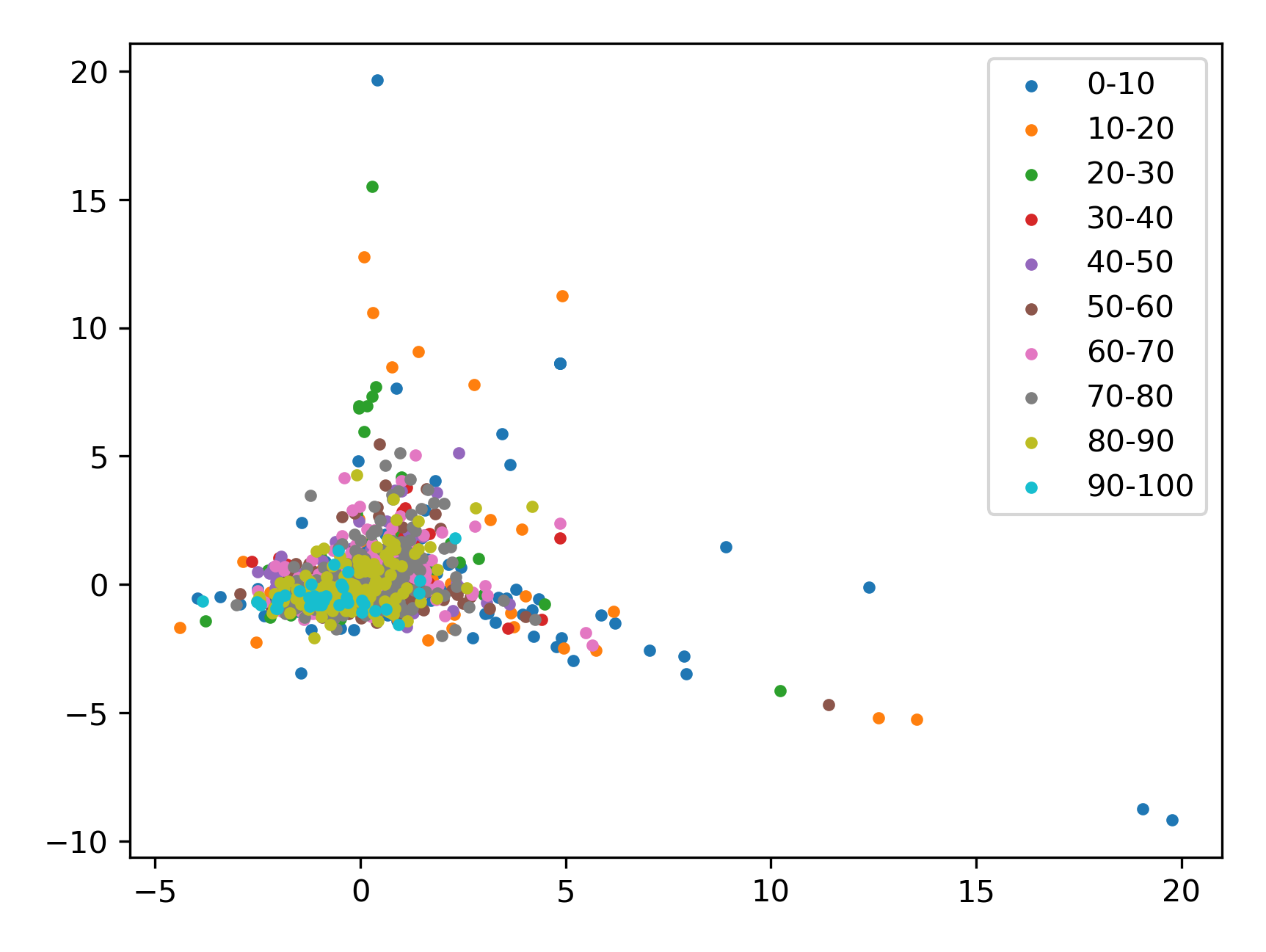
Figure 4: Visualization of user embedding vector

We can see that points corresponding to the most active groups (80-100) are centered near the origin, while points for the less active groups are distributed along two nearly orthogonal directions. This provides an intuitive explanation for our observations: data from groups 80-100 can boost the overall performance of most users because they roughly lie in the center of most points; but aggregating data across the less active users (0-80) degrades their own performance, because such users are extremely heterogeneous and distinct from each other.

References

• Abbasi-Yadkori et al. (2011) Yasin Abbasi-Yadkori, Dávid Pál, and Csaba Szepesvári. Improved algorithms for linear stochastic bandits. In NIPS, volume 11, pages 2312–2320, 2011.
• Abeille and Lazaric (2017) Marc Abeille and Alessandro Lazaric. Linear thompson sampling revisited. In Artificial Intelligence and Statistics, pages 176–184. PMLR, 2017.
• Agrawal and Goyal (2013) Shipra Agrawal and Navin Goyal. Thompson sampling for contextual bandits with linear payoffs. In International Conference on Machine Learning, pages 127–135. PMLR, 2013.
• Cantador et al. (2011) Iván Cantador, Peter Brusilovsky, and Tsvi Kuflik. 2nd workshop on information heterogeneity and fusion in recommender systems (hetrec 2011). In Proceedings of the 5th ACM conference on Recommender systems, RecSys 2011, New York, NY, USA, 2011. ACM.
• Cesa-Bianchi et al. (2013) Nicolo Cesa-Bianchi, Claudio Gentile, and Giovanni Zappella. A gang of bandits. In Advances in Neural Information Processing Systems, pages 737–745, 2013.
• Dubey and Pentland (2020) Abhimanyu Dubey and Alex Pentland. Differentially-private federated linear bandits. arXiv preprint arXiv:2010.11425, 2020.
• Durand et al. (2018) Audrey Durand, Charis Achilleos, Demetris Iacovides, Katerina Strati, Georgios D Mitsis, and Joelle Pineau. Contextual bandits for adapting treatment in a mouse model of de novo carcinogenesis. In Machine learning for healthcare conference, pages 67–82. PMLR, 2018.
• Evgeniou and Pontil (2004) Theodoros Evgeniou and Massimiliano Pontil. Regularized multi–task learning. In Proceedings of the tenth ACM SIGKDD international conference on Knowledge discovery and data mining, pages 109–117, 2004.
• Gentile et al. (2014) Claudio Gentile, Shuai Li, and Giovanni Zappella. Online clustering of bandits. In International Conference on Machine Learning, pages 757–765, 2014.
• George and Gurram (2020) Jemin George and Prudhvi Gurram. Distributed stochastic gradient descent with event-triggered communication. In Proceedings of the AAAI Conference on Artificial Intelligence, volume 34, pages 7169–7178, 2020.
• Harper and Konstan (2015) F Maxwell Harper and Joseph A Konstan. The movielens datasets: History and context. Acm transactions on interactive intelligent systems (tiis), 5(4):1–19, 2015.
• Huang et al. (2013) Junxian Huang, Feng Qian, Yihua Guo, Yuanyuan Zhou, Qiang Xu, Z Morley Mao, Subhabrata Sen, and Oliver Spatscheck. An in-depth study of lte: Effect of network protocol and application behavior on performance. ACM SIGCOMM Computer Communication Review, 43(4):363–374, 2013.
• Kia et al. (2015) Solmaz S Kia, Jorge Cortés, and Sonia Martínez. Distributed convex optimization via continuous-time coordination algorithms with discrete-time communication. Automatica, 55:254–264, 2015.
• Konečnỳ et al. (2016) Jakub Konečnỳ, H Brendan McMahan, Daniel Ramage, and Peter Richtárik. Federated optimization: Distributed machine learning for on-device intelligence. arXiv preprint arXiv:1610.02527, 2016.
• Korda et al. (2016) Nathan Korda, Balazs Szorenyi, and Shuai Li. Distributed clustering of linear bandits in peer to peer networks. In International conference on machine learning, pages 1301–1309. PMLR, 2016.
• Kveton et al. (2019) Branislav Kveton, Csaba Szepesvari, Mohammad Ghavamzadeh, and Craig Boutilier. Perturbed-history exploration in stochastic linear bandits. arXiv preprint arXiv:1903.09132, 2019.
• Li et al. (2021) Chuanhao Li, Qingyun Wu, and Hongning Wang. Unifying clustered and non-stationary bandits. In International Conference on Artificial Intelligence and Statistics, pages 1063–1071. PMLR, 2021.
• Li et al. (2010a) Lihong Li, Wei Chu, John Langford, and Robert E Schapire. A contextual-bandit approach to personalized news article recommendation. In Proceedings of the 19th international conference on World wide web, pages 661–670, 2010a.
• Li et al. (2019a) Shuai Li, Wei Chen, and Kwong-Sak Leung. Improved algorithm on online clustering of bandits. arXiv preprint arXiv:1902.09162, 2019a.
• Li et al. (2010b) Wei Li, Xuerui Wang, Ruofei Zhang, Ying Cui, Jianchang Mao, and Rong Jin. Exploitation and exploration in a performance based contextual advertising system. In Proceedings of the 16th ACM SIGKDD international conference on Knowledge discovery and data mining, pages 27–36, 2010b.
• Li et al. (2019b) Xiang Li, Kaixuan Huang, Wenhao Yang, Shusen Wang, and Zhihua Zhang. On the convergence of fedavg on non-iid data. arXiv preprint arXiv:1907.02189, 2019b.
• McMahan et al. (2017) Brendan McMahan, Eider Moore, Daniel Ramage, Seth Hampson, and Blaise Aguera y Arcas. Communication-efficient learning of deep networks from decentralized data. In Artificial Intelligence and Statistics, pages 1273–1282. PMLR, 2017.
• Smith et al. (2017) Virginia Smith, Chao-Kai Chiang, Maziar Sanjabi, and Ameet Talwalkar. Federated multi-task learning. arXiv preprint arXiv:1705.10467, 2017.
• Tropp et al. (2011) Joel Tropp et al. Freedman’s inequality for matrix martingales. Electronic Communications in Probability, 16:262–270, 2011.
• Wang et al. (2019) Yuanhao Wang, Jiachen Hu, Xiaoyu Chen, and Liwei Wang. Distributed bandit learning: Near-optimal regret with efficient communication. arXiv preprint arXiv:1904.06309, 2019.
• Wu et al. (2016) Qingyun Wu, Huazheng Wang, Quanquan Gu, and Hongning Wang. Contextual bandits in a collaborative environment. In Proceedings of the 39th International ACM SIGIR conference on Research and Development in Information Retrieval, pages 529–538. ACM, 2016.
• Yang et al. (2019) Qiang Yang, Yang Liu, Tianjian Chen, and Yongxin Tong. Federated machine learning: Concept and applications. ACM Transactions on Intelligent Systems and Technology (TIST), 10(2):1–19, 2019.
• Yi et al. (2018) Xinlei Yi, Lisha Yao, Tao Yang, Jemin George, and Karl H Johansson. Distributed optimization for second-order multi-agent systems with dynamic event-triggered communication. In 2018 IEEE Conference on Decision and Control (CDC), pages 3397–3402. IEEE, 2018.
• Zhao et al. (2018) Yue Zhao, Meng Li, Liangzhen Lai, Naveen Suda, Damon Civin, and Vikas Chandra. Federated learning with non-iid data. arXiv preprint arXiv:1806.00582, 2018.