Accelerated forward-backward method with fast convergence rate for nonsmooth convex optimization beyond differentiability

Abstract

We propose an accelerated forward-backward method with fast convergence rate for finding a minimizer of a decomposable nonsmooth convex function over a closed convex set, and name it smoothing accelerated proximal gradient (SAPG) algorithm. The proposed algorithm combines the smoothing method with the proximal gradient algorithm with extrapolation $\frac{k-1}{k+\alpha-1}$ and $\alpha>3$. The updating rule of smoothing parameter $\mu_{k}$ is a smart scheme and guarantees the global convergence rate of $o(\ln^{\sigma}k/k)$ with $\sigma\in(\frac{1}{2},1]$ on the objective function values. Moreover, we prove that the sequence is convergent to an optimal solution of the problem. Furthermore, we introduce an error term in the SAPG algorithm to get the inexact smoothing accelerated proximal gradient algorithm. And we obtain the same convergence results as the SAPG algorithm under the summability condition on the errors. Finally, numerical experiments show the effectiveness and efficiency of the proposed algorithm.

1 Introduction

A popular optimization model that encompasses various convex problems arising in scientific and engineering applications is the well-known composite minimization problem:

$$\min_{x\in\mathcal{X}}\quad f(x):=c(x)+g(x),$$ (1)

where $\mathcal{X}$ is a nonempty closed convex subset of $\mathbb{R}^{n}$, $c:\mathbb{R}^{n}\rightarrow\mathbb{R}$ is a continuous convex function on $\mathcal{X}$, and $g:\mathbb{R}^{n}\rightarrow\mathbb{R}\cup\{+\infty\}$ is a proper, lower semicontinuous convex function. For a given $\vartheta>0$, the proximal mapping of $\vartheta g$ on $\mathcal{X}$, denoted by ${\rm prox}_{\vartheta g}$, is defined by

$${\rm prox}_{\vartheta g}(y):=\arg\min_{x\in\mathcal{X}}\left\{\vartheta g(x)+\frac{1}{2}\|x-y\|^{2}\right\}.$$ (2)

The efficient computation of such a proximal mapping is indispensable to a number of functions Adly2020 ; Beck2018 ; Bian2020 ; Lu2014 . Throughout this paper, we focus on the case that the proximal operator of $g$ on $\mathcal{X}$ can be calculated effectively, and assume optimal solution set $\arg\min_{\mathcal{X}}f$ of (1) is nonempty.

In recent decades, first-order method is the leading method for solving large-scale optimization problems in real-world applications, such as compressed sensing Candes1 ; Donoho , image sciences Beck-Teboule ; Chambolle , variable selection Beck2018-MP , etc. Due to the decomposition structure of the objective function in (1), a mother scheme to solve it is the forward-backward splitting method Bruck ; Passty , which is often called the proximal gradient (PG) method when it is used to solve the convex programming. The main computational efforts of PG method in each iteration are the evaluations of the gradient of the smooth part and the proximal calculation of the other part in the objective function. Fukushima and Mine Fukushima gave an earliest work on the analysis of PG method, and recently it has been widely studied in many literatures. However, the original PG method is often slow, which is with the convergence rate of $O({1}/{k})$ on the objective function values. Then, various accelerated methods have been attempted to PG method, such as the fast iterative shrinkage-thresholding algorithm (FISTA) proposed by Beck and Teboulle Beck-Teboule , which extends the seminal work of accelerated gradient algorithm for solving a class of smooth convex minimization introduced by Nesterov in 1983 Nesterov1983 . When $c$ is continuously differentiable, a typical accelerated proximal gradient (APG) method for (1) is to perform an extrapolation on the current iteration and takes the following general form

$$\left\{\begin{aligned} &y^{k}=x^{k}+\beta_{k}(x^{k}-x^{k-1})\\ &x^{k+1}={\rm prox}_{\vartheta g}(y^{k}-\vartheta\nabla c(y^{k})),\end{aligned}\right.$$ (3)

where $\vartheta$ is a positive constant depending on the Lipschitz constant of $\nabla c$, $\{\beta_{k}\}\subseteq[0,1]$ are the extrapolation coefficients. By setting $\beta_{k}=\frac{t_{k}-1}{t_{k+1}}$ with $t_{1}=1$ and $t_{k+1}=\frac{\sqrt{t_{k}^{2}+1}+1}{2}$, FISTA exhibits a faster convergence rate of $O({1}/{k^{2}})$ on the objective function values. Based on the Nesterov’s extrapolation scheme, the accelerated process in (3) has become increasingly important and be proven to be particularly useful in the first-order methods for solving the structured convex minimization problems. Most recently, after some simplification, Chambolle and Dossal Chambolle-Dossal first proved the sequence convergence of FISTA, while it was independently settled in Attouch-MP for (3) with $\beta_{k}=\frac{k-1}{k+\alpha-1}$ and $\alpha>3$. What’s more, Attouch and Peypouquet Attouch-Peypouquet improved the convergence rate of (3) on the function values from $O(1/k^{2})$ to $o(1/k^{2})$ by setting $\alpha>3$ instead of $\alpha=3$. Besides these results, we refer the readers to Attouch2020C ; Attouch2020F ; Attouch2019 ; Attouch2020Convergence and the references therein for more complementary and interesting results on the accelerated algorithms based on the Nesterov’s extrapolation techniques.

Despite we can loose the smoothness of $g$ in (1) due to its computability of proximal operator, a crucial and standard assumption common to all the above mentioned PG and APG algorithms is the Lispchitz continuity of $\nabla c$. One may think that we can use the alternating direction of multipliers (ADM) scheme Boyd2011 ; Hong2017 ; Yang2016 when both $c$ and $g$ are nonsmooth convex function, but have the computable proximal operator. Although ADM scheme is effective for some composite models, there are several serious difficulties in doing this as discussed in Bauschke . Recently, Bauschke, Bolte and Teboulle Bauschke derived an appropriate descent lemma on replacing the upper quadratic approximation of the smooth function by a proximity measure with the Bregman distance. With this lemma, Bauschke proved that the PG algorithm owned the $O({1}/{k})$ convergence rate on the objective values when $c$ is convex and continuously differentiable (not necessarily with a global Lipschitz gradient). With some additional assumptions on the Bregman proximal distance, the sequence convergence is also established in Bauschke . Almost at the same time, Nguyen Nguyen independently analyzed the convergence of the PG method based on the Bregman distance for composite minimization problems in general reflexive Banach spaces. However, there are many problems in applications that can not be expressed by (1) with the sum of a continuously differentiable function satisfying the conditions in Bauschke and a function with computable proximal operator as the objective function. Some popular and interesting examples are listed in Section 2.

For (1) with a general nonsmooth convex objective function, there are very few literatures. Based on the method in Nesterov1983 and an appropriate smooth $\epsilon$-approximation of the initial nonsmooth objective function, Nesterov Nesterov2005 improved the efficiency estimate of the order from $O\left({1}/{\epsilon^{2}}\right)$ to $O({{1}/{\epsilon}})$ for finding an $\epsilon$-solution $x^{\epsilon}$, i.e.

$$f(x^{\epsilon})-\min f\leq\epsilon.$$

And then this work was extended to the saddle-point problem arising in finding a Nash equilibria for games with the same order of efficiency estimate Hoda . Soon after, Chen Chen-MP studied a class of smoothing methods for solving the constrained nonsmooth nonconvex optimization problem. Based on the smoothing method in Chen-MP , Zhang and Chen in zhang2009 proposed a smoothing projected gradient method for minimizing a nonsmooth nonconvex problem on a closed convex feasible set, and showed that any accumulation point generated by the method is a stationary point of the problem associated with a smoothing function. Recently, Bian and Chen Bian-Chen-SINMU came up with a smoothing proximal gradient algorithm for the constrained $\ell_{0}$ penalized nonsmooth convex regression problem. In particular, the authors in Bian-Chen-SINMU established that the local convergence rate of $o(1/k^{\tau})$ with any $\tau\in(0,{1}/{2})$ on the objective function values and the iterates converges to a local minimizer of the considered problem. Similarly, inspired by the effect of smoothing method, Zhang and Chen zhang2020 proposed a smoothing active set method for linearly constrained non-Lipschitz nonconvex optimization and proved the local convergence of the method. It is worth noting that Bian in Bian2020 independently developed a smoothing fast iterative shrinkage-thresholding algorithm based on the extrapolation coefficients of FISTA for solving problem (1) and proved that the global convergence rate of the objective function values is $O(\ln k/k)$. Without the sequential convergence, only the optimality of the accumulated points of the iterates is established in Bian2020 . Many numerical algorithms based on the smoothing methods for solving the nonsmooth optimization problem have been studied extensively Chen2018A ; Liu2016A ; Xu2015S . More recently, on the basis of the regularity properties of the Moreau envelope of a proper convex lower semicontinuous function $f$, a class of APG algorithms Adly2020 ; Attouch2020C ; Attouch2020F for solving smooth convex optimization problems are extended to nonsmooth convex optimization problems. However, the resulting algorithms involve the proximal operator of $f$. We remark that the proximal operator of most objective functions doesn’t have the closed-form solution, which isn’t needed in the proposed algorithm of this paper.

For the numerical implementation of the algorithms, it is important to study the stability with respect to the computational errors or perturbations of the numerical algorithm. Being based on the well-posed dynamic systems with a small perturbation term, there are many references on the stability properties of the accelerated forward-backward algorithms with perturbation obtained by the implicit/explicit finite difference, such as Adly2020 ; Attouch-MP ; Attouch-Peypouquet ; Aujol ; Villa . It is worth emphasizing that the convergence results of these inexact algorithms are parallel to those of the algorithms in the unperturbed case under some condition on the perturbations and errors.

Note that the study on solving (1) remains some serious difficulties and challenges that we now briefly sketch two points. First, the global convergence rates of the APG method for (1) with a general (possible nonsmooth) convex function $c$ has not been extensively considered before. Though a good convergence rate on the objective function values is estimated in Nesterov2005 , any accumulation point of the algorithm in it is an $\epsilon$-solution, where $\epsilon$ is an appropriately selected fixed positive parameter in the algorithm. Second, as far as we know, the sequential convergence of APG methods for (1) in this case have not be proved before. In this paper, we specialize the study of problem (1) in the case that $c$ is a nonsmooth convex function, and aim to extend the results in Attouch-Peypouquet to a more general composite convex minimization problem modeled by (1). Our main contributions are to propose an APG algorithm for solving (1), which not only owns a fast global convergence rate on the objective values, but also possesses the sequence convergence. As a first attempt to design, we aim to introduce the efficient smoothing techniques into the APG method to overcome the nonsmoothness of $c$ in (1). The challenge of improving the convergence rate of proposed algorithm is the updating method for the smoothing parameter. After adjusting numerous times and learning the techniques on the convergence analysis in Attouch-MP ; Attouch-Peypouquet , we give an updating scheme of the smoothing parameter, which not only let the proposed algorithm own the global convergence rate of $o(\ln^{\sigma}k/k)$ with any $\sigma\in({1}/{2},1]$ on the objective function values, but also have the global sequential convergence. In particular, we consider the effect of the errors in the proposed algorithm, and give an sufficient condition on the errors to guarantee the established convergence results of the algorithm without perturbation still hold. We hope, this work will give some insight on improving the corresponding algorithms that need the Lipschitz continuous gradient as a basic assumption to more general problems in applications.

The rest of this paper is organized as follows. Section 2 gives the definition of smoothing function and some necessary preliminary results, and lists several examples of modeling with (1) in practical applications. In Section 3, we design an accelerated algorithm, named smoothing accelerated proximal gradient (SAPG) algorithm, for solving problem (1) and derive the main convergence results of it. We also discuss the stability of SPAG algorithm with respect to errors on the calculation of the gradient in this section. Section 4 demonstrates the performance of the proposed algorithm by some numerical experiments.

Notations:

Throughout the paper, $\mathbb{R}^{n}$ is a $n$ dimensional Euclidean space equipped with the scalar product $\langle\cdot,\cdot\rangle$ and the Euclidean norm $\|\cdot\|$. We define $\mathbb{N}:=\{0,1,2,\cdots\}$. $\mathbb{R}_{+}$ denotes the set of all nonnegative real numbers. The notations $\mathbb{R}_{++}$ and $\|\cdot\|_{1}$ denote the set of all positive real numbers and the $\ell_{1}$ norm, respectively. For a vector $x\in\mathbb{R}^{n}$ and a nonempty closed convex set $\mathcal{X}\subseteq\mathbb{R}^{n}$, the projection operator to set $\mathcal{X}$ at $x$ is defined by $P_{\mathcal{X}}(x):=\arg\min\{\|x-z\|:z\in\mathcal{X}\}$.

2 Preliminary results and examples

As discussed in Introduction, the main difficulty in solving (1) by the PG and APG method is the nonsmoothness of $c$. When $c$ is nonsmooth or $\nabla c$ is not globally Lipschitz continuous, an direct idea is to use the smoothing method, which plays a central role in our analysis. In this paper, we will propose an algorithm with the smoothing function defined in Bian-Chen-SINMU , which approximates the nonsmooth convex function $c$ by a class of smooth convex functions.

Definition 2.1

Bian-Chen-SINMU For convex function $c$ in (1), we call $\tilde{c}:\mathbb{R}^{n}\times\mathbb{R}_{+}\rightarrow\mathbb{R}$ a smoothing function of $c$, if $\tilde{c}$ satisfies the following conditions:

• for any fixed $\mu>0$, $\tilde{c}(\cdot,\mu)$ is continuously differentiable on $\mathbb{R}^{n}$;

• $\lim_{z\to x,\mu\downarrow 0}\tilde{c}(z,\mu)=c(x)$, $\forall x\in\mathbb{R}^{n}$;

• (gradient consistence) $\{\lim_{z\rightarrow x,\mu\downarrow 0}\nabla_{z}\tilde{c}(z,\mu)\}\subseteq\partial c(x)$, $\forall x\in\mathcal{X}$;

• for any fixed $\mu>0$, $\tilde{c}(\cdot,\mu)$ is convex on $\mathcal{X}$;

• there exists a $\kappa>0$ such that

  $$|\tilde{c}({{x}},\mu_{2})-\tilde{c}({{x}},\mu_{1})|\leq\kappa|\mu_{1}-\mu_{2}|,\quad\forall{{x}}\in\mathcal{X},\,\mu_{1},\mu_{2}\in\mathbb{R}_{++};$$ (4)

• there exists an $L>0$ such that $\nabla_{x}\tilde{c}({\cdot},\mu)$ is Lipschitz continuous on $\mathcal{X}$ with factor $L\mu^{-1}$ for any fixed $\mu\in\mathbb{R}_{++}$.

Combining properties (ii) and (v) in Definition 2.1, we have

$$|\tilde{c}(x,\mu)-c(x)|\leq\kappa\mu,\quad\forall{{x}}\in\mathcal{X},\,\mu\in\mathbb{R}_{++}.$$ (5)

The study of smooth approximations for various specialized nonsmooth functions has a long history and rich theoretical results Chen-MP ; F-P-Book ; Nesterov2005 ; Rock-Wets ; HUL93 . Items (i)-(iii) are basic conditions in the definition of smoothing function Chen-MP , which are necessary for the effectiveness of the smoothing methods in solving the corresponding nonsmooth problems. Item (iv) states that the smoothing function $\tilde{c}(\cdot,\mu)$ maintains the convexity of $c$ for any fixed $\mu\in\mathbb{R}_{++}$. Item (v) and (vi) ensure the global Lipschitz continuity of $\tilde{c}(x,\cdot)$ on $\mathbb{R}_{++}$ for any fixed $x\in\mathbb{R}^{n}$, and the global Lipschitz continuity of $\nabla_{x}\tilde{c}(\cdot,\mu)$ for any fixed $\mu\in\mathbb{R}_{++}$, respectively.

Remark 2.1

In particular, we want to mention in advance that the values of $\kappa$ and $L$ in Definition 2.1 are not needed in the following proposed algorithm, but only used in the convergence analysis.

Now, let us look at some examples in applications modeled by (1), for which we can construct a smoothing function for the first function and calculate the proximal operator for the second function in its objective function. We can also refer to Nesterov2005 for some more examples in applications.

Example 2.1

To find a sparse solution in $\mathcal{X}$ satisfying $c(x)\approx 0$, one often considers the following $\ell_{1}$ regularized sparse optimization model

$$\min_{x\in\mathcal{X}}\quad c(x)+\lambda\|x\|_{1},$$

where $c$ is the loss function to characterize the data fitting and $\lambda>0$ is the penalty parameter. Notice that the proximal operator of $\ell_{1}$ function has a closed form expression Parikh . A notable nonsmooth convex loss function in linear regression problem is the $\ell_{1}$ function, which takes the following form

$$c(x):=\|Ax-b\|_{1},$$ (6)

with $A\in\mathbb{R}^{m\times n}$ and $b\in\mathbb{R}^{m}$. As pointed out in Fan2001 , $\ell_{1}$ loss function is nonsmooth, but more robust and has stronger capability of outlier-resistant than the least square loss function in the linear regression problems. Another important application is the loss function in censored regression problem, which is often in the form of

$$c(x):=\left\|\max\{Ax,0\}-b\right\|_{q}^{q}$$ (7)

with $q\in[1,2]$. Function $c$ in (7) is also a convex but nonsmooth function. Besides, both the check loss function in penalized quantile regression Fan2014 ; Koenker and the negative log-quasi-likehood loss function Fan2001 are nonsmooth convex functions. One can consult Bian-Chen-SINMU for the construction of smoothing functions satisfying Definition 2.1, including the smoothing functions of $c$ in (6) and (7).

Example 2.2

Since $g$ can be a possible nonsmooth extended valued function, we can let $g$ be the indicator function of a closed convex subset $\mathcal{Y}$ of $\mathbb{R}^{n}$, i.e.

$$\delta_{\mathcal{Y}}(x)=\left\{\begin{aligned} &0&&\mbox{if $x\in\mathcal{Y}$}\\ &\infty&&\mbox{if $x\not\in\mathcal{Y}$}.\end{aligned}\right.$$

Here, $\delta_{\mathcal{Y}}$ is a proper, lower semicontinuous convex function, and ${\rm prox}_{\vartheta\delta_{\mathcal{Y}}}$ is the projection operator onto $\mathcal{Y}$. Then, problem (1) is reduced to the following constrained (maybe nonsmooth) convex minimization problem

$$\min_{x\in\mathcal{X}\cap\mathcal{Y}}\quad c(x).$$

Example 2.3

Consider the following constrained convex optimization problem

$$\min\quad g(x)$$ (8)

  s.t. $$x\in\mathcal{X},\,h_{i}(x)\leq 0,\,i=1,\ldots,r,$$

where $g$ and $h_{i}:\mathbb{R}^{n}\rightarrow\mathbb{R}$, $i=1,\ldots,r$, are convex functions. It is well known that most exact penalty functions are nonsmooth. Based on the exact penalty method, under some proper conditions Clarke ; Nocedal ; Bian-Xue-CS , problem (8) can be equivalent to

$$\min\quad \lambda\sum_{i=1}^{r}\max\{h_{i}(x),0\}+g(x)$$ (9)

  s.t. $$x\in\mathcal{X},$$

where $\lambda$ is an exact penalty parameter. Problem (9) is also a special case of (1) with

$$c(x):=\lambda\sum_{i=1}^{r}\max\{h_{i}(x),0\},$$

which is a nonsmooth convex function and can have a smoothing function satisfying Definition 2.1.

3 SAPG algorithm and convergence analysis

As inspired by the success in Attouch-Peypouquet , we will propose an accelerated algorithm for solving (1) based on the scheme of (3) with $\beta_{k}=\frac{k-1}{k+\alpha-1}$ and $\alpha>3$. Equipped with the smoothing function of $c$ defined in Definition 2.1, we can now develop an accelerated proximal gradient algorithm for (1) and build the global convergence analysis including the fast convergence rate on the objective function values and the sequential convergence of iterates. In particular, it owns the global convergence rate of $o(\ln^{\sigma}k/k)$ with any $\sigma\in(\frac{1}{2},1]$.

For easy of reference and correspond to its structure, we call the proposed algorithm smoothing accelerated proximal gradient (SAPG) algorithm in this paper. In this section, we always let $\tilde{c}$ a smoothing function of $c$ defined in Definition 2.1 with positive parameters $\kappa$ and $L$ in item (v) and (vi), respectively. In what follows, $\nabla\tilde{c}(x,\mu)$ means the gradient of $\tilde{c}$ with respect to $x$ for simplicity.

3.1 SAPG algorithm

Set

$$\tilde{f}(x,\mu):=\tilde{c}(x,\mu)+g(x).$$ (10)

Notice that $\tilde{f}$ can be a nonsmooth function, since we do not assume the smoothness of $g$. However, for any fixed $\mu>0$, $\tilde{f}(\cdot,\mu)$ is with the composite structure, whose first term is a Lipschitz continuously differentiable convex function and the second term is a proper lower semicontinuous convex function with computable proximal operator. This provides a possibility of adopting the PG and APG method on it. Different from the work in Nesterov2005 , which is for problem $\min_{x\in\mathcal{X}}\tilde{f}(x,\mu)$ with a fixed and appropriate selected value of $\mu$, we will let the parameter $\mu$ tend to $0$ asymptotically and give a global convergence rate on the objective function values. The updating method of $\mu$ plays a key role in the global convergence analysis and affects the convergence rate directly. We are now ready to present the proposed SAPG algorithm for solving (1). See Algorithm 1.

• Take initial point $x^{-1}=x^{0}\in\mathcal{X}$, $\mu_{0}\in\mathbb{R}_{++}$ and $\gamma_{0}>0$. Choose parameters $\eta\in(0,1)$, $\alpha>3$ and $\sigma\in\left(\frac{1}{2},1\right]$. Set $k=0$.

• Set $\hat{\gamma}_{k+1}=\gamma_{k}$ and compute

  $$y^{k}=x^{k}+\frac{k-1}{k+\alpha-1}(x^{k}-x^{k-1}),$$ (11)

  $$\mu_{k+1}=\frac{\mu_{0}}{(k+\alpha-1)\ln^{\sigma}(k+\alpha-1)}.$$ (12)

• Compute

  $$\hat{x}^{k+1}={\rm prox}_{\hat{\gamma}_{k+1}{\mu_{k+1}}g}(y^{k}-\hat{\gamma}_{k+1}\mu_{k+1}\nabla\tilde{c}(y^{k},\mu_{k+1})).$$ (13)

• If $\hat{x}^{k+1}$ satisfies

  $$\tilde{c}(\hat{x}^{k+1},\mu_{k+1})\leq\tilde{c}({y}^{k},\mu_{k+1})+ \langle\nabla\tilde{c}({y}^{k},\mu_{k+1}),\hat{x}^{k+1}-y^{k}\rangle$$ (14)

  $$+\frac{1}{2}(\hat{\gamma}_{k+1}\mu_{k+1})^{-1}\|\hat{x}^{k+1}-y^{k}\|^{2},$$

  let $\gamma_{k+1}=\hat{\gamma}_{k+1}$, $x^{k+1}=\hat{x}^{k+1}$, increment $k$ by one and return to Step 1.

Otherwise, let $\hat{\gamma}_{k+1}=\eta\hat{\gamma}_{k+1}$ and return to Step 2.

Algorithm 1 Smoothing Accelerated Proximal Gradient (SAPG) Algorithm

It is interesting to see that (11) and (13) are the iterations of general APG method for $\tilde{f}(x,\mu_{k+1})$, which indicates that the SAPG algorithm shares the same structural decomposition principle and extrapolation as the usual APG algorithm in Attouch-Peypouquet . Similar as the work in Bian-Chen-SINMU , (14) is a simple line search for verifying the adaptability of $(\hat{\gamma}_{k+1}\mu_{k+1})^{-1}$ on the Lipschitz constant of $\nabla\tilde{c}(\cdot,\mu_{k+1})$ between $y^{k}$ and $\hat{x}^{k+1}$. It should be carefully noted that smoothing parameter $\{\mu_{k}\}$ is strictly monotone decreasing and tends to $0$ as $k\to\infty$ if the SAPG algorithm is well-defined for all $k\in\mathbb{N}$.

3.2 Some basic estimations

We start with some basic preliminary estimations for the SAPG algorithm. Let $\{x^{k}\}$, $\{y^{k}\}$, $\{\gamma_{k}\}$ and $\{\mu_{k}\}$ be the sequences generated by the SAPG algorithm. Our convergence analysis follows some basic ideas in Attouch-Peypouquet and extends it to a more general nonsmooth case.

Set

$$Q(x,y,\mu,\gamma):=\tilde{c}(y,\mu)+\langle\nabla\tilde{c}(y,\mu),x-y\rangle+\frac{1}{2}(\gamma\mu)^{-1}\|x-y\|^{2}+g(x).$$

For fixed $y$, $\mu$ and $\gamma$, $Q(\cdot,y,\mu,\gamma)$ is strongly convex with modulus $(\gamma\mu)^{-1}$, and admits a unique global minimizer on $\mathcal{X}$, which is denoted by $p(y,\mu,\gamma)$, i.e.

$$p(y,\mu,\gamma):=\arg\min_{x\in\mathcal{X}}Q(x,y,\mu,\gamma).$$

Then, it ensures that

$$Q(x,y,\mu,\gamma)\geq Q(p(y,\mu,\gamma),y,\mu,\gamma)+\frac{1}{2}(\gamma\mu)^{-1}\|x-p(y,\mu,\gamma)\|^{2},\quad\forall x\in\mathcal{X}.$$ (15)

Invoking the formulation of proximal operator in (2), (13) can be expressed as

$$\hat{x}^{k+1}=p(y^{k},\mu_{k+1},\gamma_{k+1}).$$ (16)

Lemma 3.1

The SAPG algorithm is well-defined. Moreover, the sequences $\{x^{k}\}$, $\{\gamma_{k}\}$ and $\{\mu_{k}\}$ satisfy

• $\{\gamma_{k}\}$ is non-increasing and lower bounded by $\underline{\gamma}:=\min\{{\gamma}_{0},\eta L^{-1}\}$;

• $\{\mu_{k}\}$ is monotone decreasing and $\lim_{k\rightarrow\infty}\mu_{k}=0$;

• for any $k\geq 0$, $x^{k}\in\mathcal{X}$.

Proof

Invoking Definition 2.1-(vi), (14) holds when $\gamma_{k+1}^{-1}\geq L$, which implies that the total updating iterations for returning to step 2 is at most $1+[-\log_{\eta}(L{\gamma}_{0})]$ times, where $[a]$ means the largest positive integer such that $[a]\leq a$. Combining this with (16), the SAPG algorithm is well-defined and that $\gamma_{k}\geq\underline{\gamma}:=\min\{{\gamma}_{0},\eta L^{-1}\}$.

From (12) and (13), we can directly verify the results in items (ii) and (iii).

Lemma 3.2

For any $x\in\mathcal{X}$ and $k\in\mathbb{N}$, it holds that

$$\tilde{f}(x^{k+1},\mu_{k+1})\leq \tilde{f}(x,\mu_{k+1})+(\gamma_{k+1}\mu_{k+1})^{-1}\langle y^{k}-x^{k+1},y^{k}-x\rangle$$ (17)

$$-\frac{1}{2}(\gamma_{k+1}\mu_{k+1})^{-1}\|x^{k+1}-y^{k}\|^{2}.$$

Proof

Letting $y=y^{k}$, $\mu=\mu_{k+1}$ and $\gamma=\gamma_{k+1}$ in (15), we have

$$Q(x,y^{k},\mu_{k+1},\gamma_{k+1})$$

$$\geq Q(p(y^{k},\mu_{k+1},\gamma_{k+1}),y^{k},\mu_{k+1},\gamma_{k+1})+\frac{1}{2}(\gamma_{k+1}\mu_{k+1})^{-1}\|x-p(y^{k},\mu_{k+1},\gamma_{k+1})\|^{2}$$

$$= Q(x^{k+1},y^{k},\mu_{k+1},\gamma_{k+1})+\frac{1}{2}(\gamma_{k+1}\mu_{k+1})^{-1}\|x-x^{k+1}\|^{2},\quad\forall x\in\mathcal{X}.$$

Upon rearranging the terms, we deduce that, for any $x\in\mathcal{X}$,

$$g(x^{k+1})\leq g(x)+\langle\nabla\tilde{c}(y^{k},\mu_{k+1}),x-x^{k+1}\rangle+\frac{1}{2}(\gamma_{k+1}\mu_{k+1})^{-1}\|x-y^{k}\|^{2}$$ (18)

$$-\frac{1}{2}(\gamma_{k+1}\mu_{k+1})^{-1}\|x-x^{k+1}\|^{2}-\frac{1}{2}(\gamma_{k+1}\mu_{k+1})^{-1}\|x^{k+1}-y^{k}\|^{2}.$$

Recalling (14) with $\gamma_{k+1}=\hat{\gamma}_{k+1}$ and $x^{k+1}=\hat{x}^{k+1}$, we find

$$\tilde{c}(x^{k+1},\mu_{k+1})$$ (19)

$$\leq \tilde{c}(y^{k},\mu_{k+1})+\langle\nabla\tilde{c}(y^{k},\mu_{k+1}),x^{k+1}-y^{k}\rangle+\frac{1}{2}(\gamma_{k+1}\mu_{k+1})^{-1}\|x^{k+1}-y^{k}\|^{2}.$$

Adding (18) and (19) together, we deduce that, for any $x\in\mathcal{X}$,

$$\tilde{f}(x^{k+1},\mu_{k+1})=\tilde{c}(x^{k+1},\mu_{k+1})+g(x^{k+1})$$ (20)

$$\leq \tilde{c}(y^{k},\mu_{k+1})+\langle\nabla\tilde{c}(y^{k},\mu_{k+1}),x-y^{k}\rangle+\frac{1}{2}(\gamma_{k+1}\mu_{k+1})^{-1}\|x-y^{k}\|^{2}$$

$$-\frac{1}{2}(\gamma_{k+1}\mu_{k+1})^{-1}\|x-x^{k+1}\|^{2}+g(x)$$

$$\leq \tilde{c}(x,\mu_{k+1})+g(x)+\frac{1}{2}(\gamma_{k+1}\mu_{k+1})^{-1}\|x-y^{k}\|^{2}-\frac{1}{2}(\gamma_{k+1}\mu_{k+1})^{-1}\|x-x^{k+1}\|^{2}$$

$$= \tilde{f}(x,\mu_{k+1})+\frac{1}{2}(\gamma_{k+1}\mu_{k+1})^{-1}\|x-y^{k}\|^{2}-\frac{1}{2}(\gamma_{k+1}\mu_{k+1})^{-1}\|x-x^{k+1}\|^{2},$$

where the second inequality follows from the convexity of $\tilde{c}(\cdot,\mu_{k+1})$ assumed in Definition 2.1-(iv). Thus, the rearranging terms of (20) gives (17).

Fix $x^{*}\in\arg\min_{x\in\mathcal{X}}f$. Let us bring forward the global energy function that will serve for the Lyapunov analysis:

$$\mathcal{E}_{k}:= \frac{2\gamma_{k}\mu_{k}}{\alpha-1}(k+\alpha-2)^{2}W_{k}+(\alpha-1)\|u^{k}-x^{*}\|^{2}$$ (21)

$$+\left(\frac{4\kappa{\gamma}_{0}\mu_{0}}{2\sigma-1}\right)\mu_{k}(k+\alpha-2)\ln^{1-\sigma}(k+\alpha-2),$$

where

$$W_{k}:=\tilde{f}(x^{k},\mu_{k})+\kappa\mu_{k}-f(x^{*})\quad\mbox{and}\quad u^{k}:=\left(\frac{k+\alpha-2}{\alpha-1}\right)x^{k}-\left(\frac{k-1}{\alpha-1}\right)x^{k-1}.$$ (22)

The following proposition gives a key estimation for the forthcoming analysis. It provides the most important thing that $\{\mathcal{E}_{k}\}$ is non-increasing for all $k$.

Proposition 3.1

Let $\mathcal{E}_{k}$ be the sequence defined in (21). Then, for any $k\geq 1$, we have

$$\mathcal{E}_{k+1}+\frac{2(\alpha-3)\gamma_{k+1}\mu_{k+1}}{\alpha-1}(k+\alpha-1)W_{k}\leq\mathcal{E}_{k}.$$ (23)

Moreover,

• the sequence $\{\mathcal{E}_{k}\}$ is non-increasing for all $k\geq 1$, and $\lim_{k\rightarrow\infty}\mathcal{E}_{k}$ exists;

• for every $k\geq 1$,

  $$\mathcal{E}_{k}\leq(\alpha-1)\|x^{*}-x^{0}\|^{2}+4(\alpha-1)\kappa\gamma_{0}\mu_{0}^{2}+\frac{4\kappa{\gamma}_{0}\mu_{0}^{2}}{2\sigma-1}(\alpha-1)\ln^{1-\sigma}(\alpha-1).$$

Proof

(i). Let us write inequality (17) at $x=x^{k}$ and $x=x^{*}$, respectively, i.e.

$$\tilde{f}(x^{k+1},\mu_{k+1})\leq \tilde{f}(x^{k},\mu_{k+1})+(\gamma_{k+1}\mu_{k+1})^{-1}\langle y^{k}-x^{k+1},y^{k}-x^{k}\rangle$$ (24)

$$-\frac{1}{2}(\gamma_{k+1}\mu_{k+1})^{-1}\|x^{k+1}-y^{k}\|^{2}$$

and

$$\tilde{f}(x^{k+1},\mu_{k+1})\leq \tilde{f}(x^{*},\mu_{k+1})+(\gamma_{k+1}\mu_{k+1})^{-1}\langle y^{k}-x^{k+1},y^{k}-x^{*}\rangle$$ (25)

$$-\frac{1}{2}(\gamma_{k+1}\mu_{k+1})^{-1}\|x^{k+1}-y^{k}\|^{2}.$$

Substituting the algebraic inequalities (4) and (5) into (24) and (25), respectively, we have the following two inequalities

$$W_{k+1}\leq W_{k}+(\gamma_{k+1}\mu_{k+1})^{-1}\langle y^{k}-x^{k+1},y^{k}-x^{k}\rangle$$ (26)

$$-\frac{1}{2}(\gamma_{k+1}\mu_{k+1})^{-1}\|x^{k+1}-y^{k}\|^{2}$$

and

$$W_{k+1}\leq (\gamma_{k+1}\mu_{k+1})^{-1}\langle y^{k}-x^{k+1},y^{k}-x^{*}\rangle$$ (27)

$$-\frac{1}{2}(\gamma_{k+1}\mu_{k+1})^{-1}\|x^{k+1}-y^{k}\|^{2}+2\kappa\mu_{k+1}.$$

Multiplying (26) by $\frac{k}{k+\alpha-1}$, and (27) by $\frac{\alpha-1}{k+\alpha-1}$, then adding them together, we obtain that

$$W_{k+1}\leq \frac{k}{k+\alpha-1}W_{k}+\frac{2\kappa(\alpha-1)}{k+\alpha-1}\mu_{k+1}-\frac{1}{2}(\gamma_{k+1}\mu_{k+1})^{-1}\|x^{k+1}-y^{k}\|^{2}$$ (28)

$$+(\gamma_{k+1}\mu_{k+1})^{-1}\left\langle y^{k}-x^{k+1},\frac{k}{k+\alpha-1}(y^{k}-x^{k})+\frac{\alpha-1}{k+\alpha-1}(y^{k}-x^{*})\right\rangle.$$

By using the algebraic inequality

$$-\|a-b\|^{2}+2\langle b-a,b-c\rangle=-\|a-c\|^{2}+\|b-c\|^{2}$$ (29)

with $a=x^{k+1}$, $b=y^{k}$ and $c=\frac{k}{k+\alpha-1}x^{k}+\frac{\alpha-1}{k+\alpha-1}x^{*}$, we observe that

$$-\|x^{k+1}-y^{k}\|^{2}+2\left\langle y^{k}-x^{k+1},y^{k}-\frac{k}{k+\alpha-1}x^{k}-\frac{\alpha-1}{k+\alpha-1}x^{*}\right\rangle$$ (30)

$$= -\left\|x^{k+1}-\frac{k}{k+\alpha-1}x^{k}-\frac{\alpha-1}{k+\alpha-1}x^{*}\right\|^{2}+\left\|y^{k}-\frac{k}{k+\alpha-1}x^{k}-\frac{\alpha-1}{k+\alpha-1}x^{*}\right\|^{2}$$

$$= -\left(\frac{\alpha-1}{k+\alpha-1}\right)^{2}\left(\left\|u^{k+1}-x^{*}\right\|^{2}-\left\|u^{k}-x^{*}\right\|^{2}\right),$$

where the last equality uses the expression of $y^{k}$ in (11). Substituting (30) into (28) and by simple algebraic manipulations, we have

$$W_{k+1}\leq \frac{k}{k+\alpha-1}W_{k}+\frac{2\kappa(\alpha-1)}{k+\alpha-1}\mu_{k+1}$$

$$-\frac{1}{2}(\gamma_{k+1}\mu_{k+1})^{-1}\left(\frac{\alpha-1}{k+\alpha-1}\right)^{2}\left(\|u^{k+1}-x^{*}\|^{2}-\|u^{k}-x^{*}\|^{2}\right).$$

Multiplying the above inequality by $\frac{2\gamma_{k+1}\mu_{k+1}}{\alpha-1}(k+\alpha-1)^{2}$, we obtain

$$\frac{2\gamma_{k+1}\mu_{k+1}}{\alpha-1}(k+\alpha-1)^{2}W_{k+1}\leq \frac{2\gamma_{k+1}\mu_{k+1}}{\alpha-1}k(k+\alpha-1)W_{k}+4\kappa({k+\alpha-1})\gamma_{k+1}\mu_{k+1}^{2}$$ (31)

$$-(\alpha-1)\left(\|u^{k+1}-x^{*}\|^{2}-\|u^{k}-x^{*}\|^{2}\right).$$

Since $\alpha>3$, we infer that

$$k(k+\alpha-1)= (k+\alpha-2)^{2}-(\alpha-3)(k+\alpha-1)-1$$ (32)

$$< (k+\alpha-2)^{2}-(\alpha-3)(k+\alpha-1).$$

Then, reformulating (31) by (32) yields

$$\frac{2\gamma_{k+1}\mu_{k+1}}{\alpha-1}(k+\alpha-1)^{2}W_{k+1}+\frac{2(\alpha-3)\gamma_{k+1}\mu_{k+1}}{\alpha-1}(k+\alpha-1)W_{k}$$ (33)

$$\quad+(\alpha-1)\|u^{k+1}-x^{*}\|^{2}$$

$$\leq \frac{2\gamma_{k+1}\mu_{k+1}}{\alpha-1}(k+\alpha-2)^{2}W_{k}+(\alpha-1)\|u^{k}-x^{*}\|^{2}+4\kappa({k+\alpha-1})\gamma_{k+1}\mu_{k+1}^{2}$$

$$\leq \frac{2\gamma_{k}\mu_{k}}{\alpha-1}(k+\alpha-2)^{2}W_{k}+(\alpha-1)\|u^{k}-x^{*}\|^{2}+4\kappa{\gamma}_{0}({k+\alpha-1})\mu_{k+1}^{2},$$

where the last inequality uses the non-increasing property of $\{\gamma_{k}\}$ and $\{\mu_{k}\}$. To write (33) in a recursive form, by the definition of $\mu_{k}$ given in (12), we observe that

$$\mu_{0}\mu_{k}(k+\alpha-2)\ln^{1-\sigma}(k+\alpha-2)-\mu_{0}\mu_{k+1}(k+\alpha-1)\ln^{1-\sigma}(k+\alpha-1)$$ (34)

$$= \mu_{0}^{2}\left(\ln^{1-2\sigma}(k+\alpha-2)-\ln^{1-2\sigma}(k+\alpha-1)\right)$$

$$= \frac{\mu_{0}^{2}}{\ln^{2\sigma-1}(k+\alpha-1)}\left(\frac{\ln^{2\sigma-1}(k+\alpha-1)}{\ln^{2\sigma-1}(k+\alpha-2)}-1\right)$$

$$\geq (2\sigma-1)(k+\alpha-1)\mu_{k+1}^{2}\frac{\ln^{2\sigma-1}(k+\alpha-1)}{\ln^{2\sigma-1}(k+\alpha-2)}$$

$$\geq (2\sigma-1)(k+\alpha-1)\mu_{k+1}^{2},$$

where the third inequality follows from

$$\ln^{2\sigma-1}(k+\alpha-1)\geq\ln^{2\sigma-1}(k+\alpha-2)+(2\sigma-1)\frac{\ln^{2\sigma-2}(k+\alpha-1)}{(k+\alpha-1)},\quad\forall\sigma\in\left(\frac{1}{2},1\right].$$

Combining (33) with (34), we finish the proof for the estimation in (23). Thus, $\{\mathcal{E}_{k}\}$ is non-increasing for $k\geq 1$, i.e. $\mathcal{E}_{k}\leq\mathcal{E}_{1}$.

By (5) and $x^{k}\in\mathcal{X}$, we get

$$W_{k}=\tilde{f}(x^{k},\mu_{k})+\kappa\mu_{k}-f(x^{*})\geq f(x^{k})-f(x^{*})\geq 0,$$ (35)

then $\mathcal{E}_{k}$ is lower bounded by $0$, which implies the existence of $\lim_{k\rightarrow\infty}\mathcal{E}_{k}$.

(ii). According to the non-increasing of sequence $\{\mathcal{E}_{k}\}$, then, all that remains is to estimate the upper bound of

$$\mathcal{E}_{1}=2\gamma_{1}\mu_{1}(\alpha-1)W_{1}+(\alpha-1)\|u^{1}-x^{*}\|^{2}+\frac{4\kappa{\gamma}_{0}\mu_{0}}{2\sigma-1}\mu_{1}(\alpha-1)\ln^{1-\sigma}(\alpha-1).$$ (36)

Returning to (27) with $k=0$, and using (29), we deduce that

$$W_{1}\leq (\gamma_{1}\mu_{1})^{-1}\langle y^{0}-x^{1},y^{0}-x^{*}\rangle-\frac{1}{2}(\gamma_{1}\mu_{1})^{-1}\|x^{1}-y^{0}\|^{2}+2\kappa\mu_{1}$$

$$= \frac{1}{2}(\gamma_{1}\mu_{1})^{-1}\|x^{*}-y^{0}\|^{2}-\frac{1}{2}(\gamma_{1}\mu_{1})^{-1}\|x^{*}-x^{1}\|^{2}+2\kappa\mu_{1},$$

which implies

$$2\gamma_{1}\mu_{1}W_{1}+\|x^{*}-x^{1}\|^{2}\leq\|x^{*}-y^{0}\|^{2}+4\kappa\gamma_{1}\mu_{1}^{2}.$$ (37)

Recalling the definition of $u^{1}$ in (22), we see that $u^{1}=x^{1}$, combining which with (36), (37), $y^{0}=x^{0}$, $\mu_{1}<\mu_{0}$ and $\gamma_{1}\leq\gamma_{0}$, we find that

$$\mathcal{E}_{1}\leq(\alpha-1)\|x^{*}-x^{0}\|^{2}+4(\alpha-1)\kappa\gamma_{0}\mu_{0}^{2}+\frac{4\kappa{\gamma}_{0}\mu_{0}^{2}}{2\sigma-1}(\alpha-1)\ln^{1-\sigma}(\alpha-1).$$ (38)

Hence, we establish the evaluation in item (ii).

As a result of Proposition 3.1, we obtain some important properties of $W_{k}$ as shown below, where we need introduce an important lemma on sequence convergence.

Lemma 3.3

Attouch-MP Let $\{a_{k}\}$ be a sequence of nonnegative numbers, and satisfy

$$\sum_{k=1}^{\infty}(a_{k+1}-a_{k})_{+}<\infty.$$

Then, $\lim_{k\to\infty}a_{k}$ exists.

Proposition 3.2

Let $\{W_{k}\}$ be the sequence defined in (22), then

• $\sum_{k=1}^{\infty}\gamma_{k}\mu_{k}(k+\alpha-2)W_{k}<\infty$;

• $\lim_{k\rightarrow\infty}\left[(k-1)^{2}\|x^{k}-x^{k-1}\|^{2}+2\gamma_{k}\mu_{k}(k+\alpha-2)^{2}W_{k}\right]$ exists;

• $\sum_{k=1}^{\infty}(k-1)\|x^{k}-x^{k-1}\|^{2}<\infty$.

Proof

(i). By summing up inequality (23) from $k=1$ to $K$, we see that

$$\mathcal{E}_{K+1}+\frac{2(\alpha-3)}{\alpha-1}\sum_{k=1}^{K}\gamma_{k+1}\mu_{k+1}(k+\alpha-1)W_{k}\leq\mathcal{E}_{1}.$$

After letting $K$ tend to infinity in the above inequality and using (38), since $\alpha>3$ and $\mathcal{E}_{k}\geq 0$ for all $k\geq 0$, we infer that

$$\sum_{k=1}^{\infty}\gamma_{k+1}\mu_{k+1}(k+\alpha-1)W_{k}\leq\frac{(\alpha-1)\mathcal{E}_{1}}{2(\alpha-3)}<\infty.$$ (39)

Since, for all $k\geq 1$, it holds that

$$\gamma_{k+1}\mu_{k+1}(k+\alpha-1)=\gamma_{k+1}\frac{\mu_{0}}{\ln^{\sigma}(k+\alpha-1)}\geq \underline{\gamma}\mu_{k}\frac{(k+\alpha-2)\ln^{\sigma}(k+\alpha-2)}{\ln^{\sigma}(k+\alpha-1)}$$ (40)

$$\geq \frac{\underline{\gamma}\ln^{\sigma}(\alpha-1)}{\gamma_{0}\ln^{\sigma}\alpha}\gamma_{k}\mu_{k}(k+\alpha-2),$$

which uses $\underline{\gamma}\leq\gamma_{k}\leq\gamma_{0}$ proved in Lemma 3.1 and the increasing of $\frac{\ln^{\sigma}(k+\alpha-2)}{\ln^{\sigma}(k+\alpha-1)}$ for all $k\geq 1$, then (39) implies

$$\sum_{k=1}^{\infty}\gamma_{k}\mu_{k}(k+\alpha-2)W_{k}<\infty.$$

(ii). Returning to (26) and using (29) with $a=x^{k+1}$, $b=y^{k}$ and $c=x^{k}$, we deduce that

$$W_{k+1}\leq W_{k}-\frac{1}{2}(\gamma_{k+1}\mu_{k+1})^{-1}\|x^{k+1}-x^{k}\|^{2}+\frac{1}{2}(\gamma_{k+1}\mu_{k+1})^{-1}\|y^{k}-x^{k}\|^{2}.$$

In view of the definition of $y^{k}$ in (11), we have from multiplying $2\gamma_{k+1}\mu_{k+1}(k+\alpha-1)^{2}$ on the above inequality that

$$2\gamma_{k+1}\mu_{k+1}(k+\alpha-1)^{2}W_{k+1}+(k+\alpha-1)^{2}\|x^{k+1}-x^{k}\|^{2}$$ (41)

$$\leq 2\gamma_{k+1}\mu_{k+1}(k+\alpha-1)^{2}W_{k}+(k-1)^{2}\|x^{k}-x^{k-1}\|^{2}.$$

By $k+\alpha-1\geq k$ and upon rearranging terms of the above inequality, it suffices to observe that

$$0\geq k^{2}\|x^{k+1}-x^{k}\|^{2}-(k-1)^{2}\|x^{k}-x^{k-1}\|^{2}$$ (42)

$$+2\gamma_{k+1}\mu_{k+1}(k+\alpha-1)^{2}(W_{k+1}-W_{k}).$$

Notice that

$$\mu_{k+1}(k+\alpha-1)^{2}-\mu_{k}(k+\alpha-2)^{2}$$

$$= \mu_{k+1}(k+\alpha-1)\left(k+\alpha-1-\frac{(k+\alpha-2)\ln^{\sigma}(k+\alpha-1)}{\ln^{\sigma}(k+\alpha-2)}\right)$$

$$\leq \mu_{k+1}(k+\alpha-1),$$

then

$$\mu_{k+1}(k+\alpha-1)^{2}W_{k+1}-\mu_{k}(k+\alpha-2)^{2}W_{k}$$ (43)

$$= \mu_{k+1}(k+\alpha-1)^{2}\left(W_{k+1}-W_{k}\right)+\left(\mu_{k+1}(k+\alpha-1)^{2}-\mu_{k}(k+\alpha-2)^{2}\right)W_{k}$$

$$\leq \mu_{k+1}(k+\alpha-1)^{2}\left(W_{k+1}-W_{k}\right)+\mu_{k+1}(k+\alpha-1)W_{k}.$$

For simplicity of notation, denote

$$\alpha_{k}:=(k-1)^{2}\|x^{k}-x^{k-1}\|^{2}+2\gamma_{k}\mu_{k}(k+\alpha-2)^{2}W_{k}.$$ (44)

Substituting (43) into (42), by $\gamma_{k+1}\leq\gamma_{k}$, and upon rearranging the terms, we deduce that

$$\alpha_{k+1}-\alpha_{k}\leq 2\gamma_{k+1}\mu_{k+1}(k+\alpha-1)W_{k}.$$ (45)

Taking the positive part of the left-hand and thanks to (39), we find

$$\sum_{k=1}^{\infty}(\alpha_{k+1}-\alpha_{k})_{+}<\infty.$$

Since $\alpha_{k}\geq 0$, by Lemma 3.3, we infer that

$$\lim_{k\rightarrow\infty}\alpha_{k}\quad\mbox{exists}.$$

(iii). In view of $\alpha>3$, we observe that

$$(k+\alpha-1)^{2}\|x^{k+1}-x^{k}\|^{2}-(k-1)^{2}\|x^{k}-x^{k-1}\|^{2}$$

$$\geq (k+2)^{2}\|x^{k+1}-x^{k}\|^{2}-(k-1)^{2}\|x^{k}-x^{k-1}\|^{2}$$

$$\geq k^{2}\|x^{k+1}-x^{k}\|^{2}-(k-1)^{2}\|x^{k}-x^{k-1}\|^{2}+4k\|x^{k+1}-x^{k}\|^{2},$$

combining which with (45), then we obtain

$$k^{2}\|x^{k+1}-x^{k}\|^{2}-(k-1)^{2}\|x^{k}-x^{k-1}\|^{2}+4k\|x^{k+1}-x^{k}\|^{2}$$

$$\leq 2\gamma_{k}\mu_{k}(k+\alpha-2)^{2}W_{k}-2\gamma_{k+1}\mu_{k+1}(k+\alpha-1)^{2}W_{k+1}+2\gamma_{k+1}\mu_{k+1}(k+\alpha-1)W_{k}.$$

Summing up the above inequality for $k=1,2,\ldots,K$, we obtain

$$K^{2}\|x^{K+1}-x^{K}\|^{2}+4\sum_{k=1}^{K}k\|x^{k+1}-x^{k}\|^{2}$$ (46)

$$\leq 2\gamma_{1}\mu_{1}(\alpha-1)^{2}W_{1}+2\sum_{k=1}^{K}\gamma_{k+1}\mu_{k+1}(k+\alpha-1)W_{k}.$$

Since $W_{1}\leq\mathcal{E}_{1}$, letting $K$ tend to infinity in the above inequality, by (39) and (46), we have $\sum_{k=1}^{\infty}k\|x^{k+1}-x^{k}\|^{2}<\infty$.

3.3 Convergence rate for the objective values

Thanks to the above analysis, we are now ready to give the global convergence rate of $f(x^{k})$ to $\min_{\mathcal{X}}f$.

Theorem 3.1

Let $\{x^{k}\}$ be the sequence generated by the SAPG algorithm. Then,

$$\lim_{k\rightarrow\infty}(k+\alpha-2)\ln^{-\sigma}(k+\alpha-1)(f(x^{k})-\min_{\mathcal{X}}f)=0$$ (47)

and

$$\liminf_{k\rightarrow\infty}(k+\alpha-2)\ln^{1-\sigma}(k+\alpha-2)(f(x^{k})-\min_{\mathcal{X}}f)=0.$$ (48)

Proof

Combining (i) and (iii) in Proposition 3.2, we have

$$\sum_{k=1}^{\infty}\left[(k-1)\|x^{k}-x^{k-1}\|^{2}+2\gamma_{k}\mu_{k}(k+\alpha-2)W_{k}\right]<\infty,$$

which implies

$$\sum_{k=1}^{\infty}\frac{\ln(k+\alpha-2)}{(k+\alpha-2)\ln(k+\alpha-2)}\left[(k-1)^{2}\|x^{k}-x^{k-1}\|^{2}+2\gamma_{k}\mu_{k}(k+\alpha-2)^{2}W_{k}\right]$$

$$\leq \sum_{k=1}^{\infty}\frac{1}{k+\alpha-2}\left[(k-1)(k+\alpha-2)\|x^{k}-x^{k-1}\|^{2}+2\gamma_{k}\mu_{k}(k+\alpha-2)^{2}W_{k}\right]$$

$$= \sum_{k=1}^{\infty}\left[(k-1)\|x^{k}-x^{k-1}\|^{2}+2\gamma_{k}\mu_{k}(k+\alpha-2)W_{k}\right]<\infty.$$

Observe that $\sum_{k=1}^{\infty}\frac{1}{(k+\alpha-1)\ln(k+\alpha-1)}=\infty$, then

$$\liminf_{k\rightarrow\infty}\ln(k+\alpha-2)\left((k-1)^{2}\|x^{k}-x^{k-1}\|^{2}+2\gamma_{k}\mu_{k}(k+\alpha-2)^{2}W_{k}\right)=0.$$ (49)

Combining this with Proposition 3.2-(ii), we obtain

$$\lim_{k\rightarrow\infty}(k-1)^{2}\|x^{k}-x^{k-1}\|^{2}+2\gamma_{k}\mu_{k}(k+\alpha-2)^{2}W_{k}=0,$$ (50)

by $W_{k}\geq 0$, which further implies

$$\lim_{k\rightarrow\infty}(k-1)^{2}\|x^{k}-x^{k-1}\|^{2}=0\quad\mbox{and}\quad\lim_{k\rightarrow\infty}\gamma_{k}\mu_{k}(k+\alpha-2)^{2}W_{k}=0.$$ (51)

Recalling the definition of $\mu_{k}$ in (12), $\gamma_{k}\geq\underline{\gamma}>0$ and (35), the second equation in (51) implies (47). Similarly, (49) gives (48).

(47) in Theorem 3.1 illustrates that for any $\sigma\in(\frac{1}{2},1]$ in the SAPG algorithm, it holds $f(x^{k})-\min_{\mathcal{X}}f=o(\ln^{\sigma}k/k)$.

3.4 Sequential convergence

In this subsection, we begin to analyze the convergence of the iterates generated by the SAPG algorithm

Opial’s Lemma was first used to analyze the convergence of nonlinear contraction semigroups Bruck1975 . Here, we state the discrete version of it to prepare for analyzing the convergence of sequence.

Lemma 3.4

opial Let $S$ be a nonempty subset of $\mathbb{R}^{n}$ and $\{z_{k}\}$ be a sequence of $\mathbb{R}^{n}$. Assume that

• $\lim_{k\to\infty}\|z_{k}-z\|$ exists for every $z\in S$;

• every sequential limit point of sequence $\{z_{k}\}$ as $k\to\infty$ belongs to $S$.

Then, as $k\to\infty$, $\{z_{k}\}$ converges to a point in $S$.

To prove the sequential convergence, we also need recall the following inequality on nonnegative sequences, which will be used in the forthcoming sequential convergence result.

Lemma 3.5

Attouch-MP Assume $\alpha\geq 3$. Let $\{a_{k}\}$ and $\{\omega_{k}\}$ be two sequences of nonnegative numbers such that

$$a_{k+1}\leq\frac{k-1}{k+\alpha-1}a_{k}+\omega_{k}$$

for all $k\geq 1$. If $\sum_{k=1}^{\infty}k\omega_{k}<\infty$, then $\sum_{k=1}^{\infty}a_{k}<\infty$.

Theorem 3.2

(Sequential convergence) Let $\{x^{k}\}$ be the sequence generated by the SAPG algorithm. Then, $\{x^{k}\}$ converges to a point belonging to $\arg\min_{\mathcal{X}}f$ as $k\rightarrow\infty$.

Proof

To apply Lemma 3.4 to prove the convergence of $\{x^{k}\}$, we first prove that any cluster point of $\{x^{k}\}$ belongs to $\arg\min_{\mathcal{X}}f$. Suppose $\bar{x}$ is a cluster point of $\{x^{k}\}$ with subsequence $\{x^{k_{j}}\}$, then by the continuity of $f$ and $\{x^{k}\}\subseteq\mathcal{X}$, we have

$$f(\bar{x})=\lim_{j\rightarrow\infty}f(x^{k_{j}})=\min_{\mathcal{X}}f,$$

which implies $\bar{x}\in\arg\min_{\mathcal{X}}f$.

Next, if we can verify that for every $x^{*}\in\arg\min_{\mathcal{X}}f$, $\lim_{k\rightarrow\infty}\|x^{k}-x^{*}\|$ exists, then we conclude the sequential convergence of $\{x^{k}\}$ by Lemma 3.4.

Set

$$h_{k}:=\|x^{k}-x^{*}\|^{2}$$ (52)

with $x^{*}\in\arg\min_{\mathcal{X}}f$. Multiplying $2\gamma_{k+1}\mu_{k+1}$ on the both sides of (27) and by $W_{k+1}\geq 0$, we obtain

$$2\langle y^{k}-x^{k+1},y^{k}-x^{*}\rangle-\|x^{k+1}-y^{k}\|^{2}+4\kappa\gamma_{k+1}\mu_{k+1}^{2}\geq 0,$$

which can be reformulated by

$$\|y^{k}-x^{*}\|^{2}-\|x^{k+1}-x^{*}\|^{2}+4\kappa\gamma_{k+1}\mu_{k+1}^{2}\geq 0.$$

Then, recalling the definition of $y^{k}$, we get

$$\|x^{k+1}-x^{*}\|^{2}\leq \|y^{k}-x^{*}\|^{2}+4\kappa\gamma_{k+1}\mu_{k+1}^{2}$$

$$= \|x^{k}-x^{*}\|^{2}+\left(\frac{k-1}{k+\alpha-1}\right)^{2}\|x^{k}-x^{k-1}\|^{2}$$

$$+2\left(\frac{k-1}{k+\alpha-1}\right)\langle x^{k}-x^{*},x^{k}-x^{k-1}\rangle+4\kappa\gamma_{k+1}\mu_{k+1}^{2}$$

$$= \|x^{k}-x^{*}\|^{2}+\left(\left(\frac{k-1}{k+\alpha-1}\right)^{2}+\left(\frac{k-1}{k+\alpha-1}\right)\right)\|x^{k}-x^{k-1}\|^{2}$$

$$+\left(\frac{k-1}{k+\alpha-1}\right)\left(\|x^{k}-x^{*}\|^{2}-\|x^{k-1}-x^{*}\|^{2}\right)+4\kappa\gamma_{k+1}\mu_{k+1}^{2}$$

$$\leq \|x^{k}-x^{*}\|^{2}+2\|x^{k}-x^{k-1}\|^{2}$$

$$+\left(\frac{k-1}{k+\alpha-1}\right)\left(\|x^{k}-x^{*}\|^{2}-\|x^{k-1}-x^{*}\|^{2}\right)+4\kappa\gamma_{k+1}\mu_{k+1}^{2},$$

which can be reformulated by

$$(h_{k+1}-h_{k})_{+}\leq\left(\frac{k-1}{k+\alpha-1}\right)(h_{k}-h_{k-1})_{+}+2\|x^{k}-x^{k-1}\|^{2}+4\kappa\gamma_{k+1}\mu_{k+1}^{2}.$$ (53)

Recalling the definition of $\mu_{k+1}$ in (12) and the non-increasing property of $\gamma_{k}$ proved in Lemma 3.1-(i), we get

$$\sum_{k=1}^{\infty}k\gamma_{k+1}\mu_{k+1}^{2}\leq\sum_{k=0}^{\infty}\gamma_{0}\frac{1}{(k+\alpha-1)\ln^{2\sigma}(k+\alpha-1)}<\infty,$$ (54)

which uses $\sigma>\frac{1}{2}$ in the last inequality.

Applying the above result in Lemma 3.5 with $a_{k}=(h_{k}-h_{k-1})_{+}$, and by Proposition 3.2-(iii), we have

$$\sum_{k=1}^{\infty}(h_{k+1}-h_{k})_{+}<\infty.$$ (55)

As a consequence, we can easily deduce the convergence of $h_{k}$ as $k\rightarrow\infty$ by the nonnegativity of $\{h_{k}\}$ and Lemma 3.3. This completes the proof.

Remark 3.1

To obtain (55), one key point is the additivity of $\sum_{k=1}^{\infty}k\mu_{k+1}^{2}$, which is guaranteed by the definition of $\mu_{k+1}$ in (12) with $\sigma>\frac{1}{2}$.

3.5 Stability

In this section, we consider an inexact version of the SAPG algorithm in Algorithm 1. The inexact version comes from the error on the computation of $\nabla\tilde{c}(y^{k},\mu_{k+1})$ and we will give a tolerance estimate for the error sequence to guarantee the all convergence properties of SAPG algorithm in Theorem 3.1 and Theorem 3.2. Here, since we allow some errors on the calculation of $\nabla\tilde{c}$, we need the prior knowledge on the Lipschitz constant of $\nabla\tilde{c}(x,\mu)$, which means that the constant $L$ in Definition 2.1-(vi) is known in advance, and we fix the parameter $\gamma_{k}:=L^{-1}$ in Algorithm 1. The inexact version of Algorithm 1 is shown in Algorithm 2 and named by inexact smoothing accelerated proximal gradient (ISAPG) algorithm, where $\epsilon_{k}\in\mathbb{R}^{n}$ is an unknown error.

• Take initial point $x^{-1}=x^{0}\in\mathcal{X}$ and $\mu_{0}\in\mathbb{R}_{++}$. Choose parameters $\alpha>3$ and $\sigma\in(\frac{1}{2},1]$.

  Set $k=0$.

• Let

  $$y^{k}=x^{k}+\frac{k-1}{k+\alpha-1}(x^{k}-x^{k-1}),$$ (56)

  $$\mu_{k+1}=\frac{\mu_{0}}{(k+\alpha-1)\ln^{\sigma}(k+\alpha-1)}.$$ (57)

• Compute

  $$x^{k+1}={\rm prox}_{L^{-1}{\mu_{k+1}}g}(y^{k}-L^{-1}\mu_{k+1}(\nabla\tilde{c}(y^{k},\mu_{k+1})+{\epsilon_{k}})).$$ (58)

Algorithm 2 Inexact Smoothing Accelerated Proximal Gradient (ISAPG) Algorithm

Notice that the Step 1 in Algorithm 1 and Algorithm 2 are same. Denote

$$Q_{k}(x,y,\mu):=\tilde{c}(y,\mu)+\langle\nabla\tilde{c}(y,\mu)+\epsilon_{k},x-y\rangle+\frac{1}{2}L\mu^{-1}\|x-y\|^{2}+g(x).$$

Then, $x^{k+1}$ in (58) is the solution of

$$\min_{x\in\mathcal{X}}Q_{k}(x,y^{k},\mu_{k+1}).$$

This means that

$$y^{k}-L^{-1}\mu_{k+1}\nabla\tilde{c}(y^{k},\mu_{k+1})\in x^{k+1}+L^{-1}\mu_{k+1}(\partial g(x^{k+1})+\epsilon_{k})+N_{\mathcal{X}}(x^{k+1}),$$

where $N_{\mathcal{X}}(x^{k+1})$ is the normal cone to $\mathcal{X}$ at $x^{k+1}$. Due to the strong convexity of $Q_{k}$ to $x$ for fixed $y$ and $\mu$, we also have

$$Q_{k}(x,y^{k},\mu_{k+1})\geq Q_{k}(x^{k+1},y^{k},\mu_{k+1})+\frac{L}{2}\mu_{k+1}^{-1}\|x-x^{k+1}\|^{2},\quad\forall x\in\mathcal{X}.$$ (59)

The analysis method of the ISAPG algorithm is similar to the unperturbed case of SAPG algorithm. Hence, we state the main results, sketch the proofs to avoid repeating similar arguments, and underline the parts where additional techniques are required. Next, we first recall the discrete version of Gronwall-Bellman lemma.

Proposition 3.3

Attouch-MP Let $\{a_{k}\}$ be a sequence of nonnegative numbers satisfying

$$a_{k}^{2}\leq c^{2}+\sum_{j=1}^{k}\beta_{j}a_{j}$$

for all $k\in\mathbb{N}$, where $c\geq 0$ and $\{\beta_{j}\}$ is a summable sequence of nonnegative numbers. Then, $a_{k}\leq c+\sum_{j=1}^{\infty}\beta_{j}$ for all $k\in\mathbb{N}$.

Theorem 3.3

Let $\{x^{k}\}$ be the sequence generated by the ISAPG algorithm. If the errors satisfy $\sum_{k=1}^{\infty}\mu_{k+1}(k+\alpha-1)\|\epsilon_{k}\|<\infty$, then

• $\sum_{k=1}^{\infty}\mu_{k}(k+\alpha-2)W_{k}<\infty$, $\sum_{k=1}^{\infty}(k-1)\|x^{k}-x^{k-1}\|^{2}<\infty$;

• $\lim_{k\rightarrow\infty}\left[(k-1)^{2}\|x^{k}-x^{k-1}\|^{2}+2L^{-1}\mu_{k}(k+\alpha-2)^{2}W_{k}\right]$ exists;

• the conclusions in Theorem 3.1 and Theorem 3.2 hold.

Proof

(i). Since (14) always holds when $\hat{\gamma}_{k+1}=L^{-1}$, similar to the proof idea of Lemma 3.1 and Lemma 3.2, it gives $x^{k}\in\mathcal{X}$, $\forall k$, $\lim_{k\rightarrow\infty}\mu_{k}=0$ and for all $x\in\mathcal{X}$,

$$\tilde{f}(x^{k+1},\mu_{k+1})$$ (60)

$$\leq \tilde{f}(x,\mu_{k+1})+\frac{1}{2}L\mu_{k+1}^{-1}\|x-y^{k}\|^{2}-\frac{1}{2}L\mu_{k+1}^{-1}\|x-x^{k+1}\|^{2}+\langle\epsilon_{k},x-x^{k+1}\rangle.$$

In what follows, the key idea for proving the results in this theorem relies on the following energy function:

$$\bar{\mathcal{E}}_{k}={\mathcal{E}}_{k}+2L^{-1}\sum_{j=k}^{\infty}\mu_{j+1}(j+\alpha-1)\langle\epsilon_{j},x^{*}-u^{j+1}\rangle,$$

where $x^{*}$, ${\mathcal{E}}_{k}$ and $u^{k}$ are defined as in (21) and (22). Following the proof ideas in Proposition 3.1, we obtain

$${\mathcal{E}}_{k+1}+\frac{2L^{-1}(\alpha-3)\mu_{k+1}}{\alpha-1}(k+\alpha-1)W_{k}\leq{\mathcal{E}}_{k}+2L^{-1}\mu_{k+1}(k+\alpha-1)\langle\epsilon_{k},x^{*}-u^{k+1}\rangle,$$

which implies

$$\bar{\mathcal{E}}_{k+1}+\frac{2L^{-1}(\alpha-3)\mu_{k+1}}{\alpha-1}(k+\alpha-1)W_{k}\leq\bar{\mathcal{E}}_{k}.$$ (61)

Then, $\{\bar{\mathcal{E}}_{k}\}$ is non-increasing and $\bar{\mathcal{E}}_{k}\leq\bar{\mathcal{E}}_{0}$, for all $k\geq 0$. By virtue of $\bar{\mathcal{E}}_{k}\leq\bar{\mathcal{E}}_{0}$ and $W_{k}\geq 0$, we obtain

$$\|u^{k}-x^{*}\|^{2}\leq \frac{1}{\alpha-1}\mathcal{E}_{0}+\frac{2L^{-1}}{\alpha-1}\sum_{j=0}^{k-1}\mu_{j+1}(j+\alpha-1)\langle\epsilon_{j},x^{*}-u^{j+1}\rangle$$

$$\leq \frac{1}{\alpha-1}\mathcal{E}_{0}+\frac{2L^{-1}}{\alpha-1}\sum_{j=1}^{k}\mu_{j}(j+\alpha-2)\|\epsilon_{j-1}\|\|u^{j}-x^{*}\|.$$

Applying Proposition 3.3 with $a_{k}=\|u^{k}-x^{*}\|$ and $\beta_{j}=\mu_{j}(j+\alpha-2)\|\epsilon_{j-1}\|$ to the above inequality, and by the condition on $\epsilon_{k}$ given in this theorem, we deduce that

$$\|u^{k}-x^{*}\|\leq\Gamma:=\sqrt{\frac{1}{\alpha-1}\mathcal{E}_{0}}+\frac{2L^{-1}}{\alpha-1}\sum_{j=1}^{\infty}\mu_{j}(j+\alpha-2)\|\epsilon_{j-1}\|,\quad\forall k\geq 0.$$ (62)

Then, the above bound with ${\mathcal{E}}_{k}\geq 0$ gives

$$\bar{\mathcal{E}}_{k}\geq-2L^{-1}\Gamma\sum_{j=k}^{\infty}\mu_{j+1}(j+\alpha-1)\|\epsilon_{j}\|>-\infty.$$

Thus, $\bar{\mathcal{E}}_{k}$ is bounded from below and (61) gives

$$\sum_{k=1}^{\infty}\mu_{k+1}(k+\alpha-1)W_{k}<\infty\quad\mbox{and}\quad\lim_{k\rightarrow\infty}\bar{\mathcal{E}}_{k}\quad\mbox{exists.}$$ (63)

By a same analysis of (40), it holds that

$$\mu_{k}(k+\alpha-2)\frac{\ln^{\sigma}(\alpha-1)}{\ln^{\sigma}\alpha}\leq\mu_{k+1}(k+\alpha-1),$$

this together with (63), we obtain $\sum_{k=1}^{\infty}\mu_{k}(k+\alpha-2)W_{k}<\infty.$

Performing a similar analysis of (41)-(43) but not loosing $k+\alpha-1$ to $k$, we have

$$(k+\alpha-1)^{2}\|x^{k+1}-x^{k}\|^{2}-(k-1)^{2}\|x^{k}-x^{k-1}\|^{2}$$ (64)

$$\quad+2L^{-1}\mu_{k+1}(k+\alpha-1)^{2}W_{k+1}-2L^{-1}\mu_{k}(k+\alpha-2)^{2}W_{k}$$

$$\leq 2L^{-1}\mu_{k+1}(k+\alpha-1)W_{k}+2L^{-1}\mu_{k+1}(k+\alpha-1)^{2}\|\epsilon_{k}\|\|x^{k}-x^{k+1}\|.$$

Summing up the above inequality for $k=1,\ldots,K$ and thanks to $W_{k}\geq 0$, we obtain

$$(K+\alpha-1)^{2}\|x^{K+1}-x^{K}\|^{2}+\sum_{k=1}^{K-1}((k+\alpha-1)^{2}-k^{2})\|x^{k+1}-x^{k}\|^{2}$$ (65)

$$\leq C^{2}+2L^{-1}\sum_{k=1}^{K}\mu_{k+1}(k+\alpha-1)^{2}\|\epsilon_{k}\|\|x^{k}-x^{k+1}\|,$$

where $C:=\sqrt{2L^{-1}(\mu_{1}(\alpha-1)^{2}W_{1}+\sum_{k=1}^{\infty}\mu_{k+1}(k+\alpha-1)W_{k})}$ is a finite number due to (63). Then, we deduce that, for $\forall K\geq 1$,

$$(K+\alpha-1)^{2}\|x^{K+1}-x^{K}\|^{2}\leq C^{2}+2L^{-1}\sum_{k=1}^{K}\mu_{k+1}(k+\alpha-1)^{2}\|\epsilon_{k}\|\|x^{k}-x^{k+1}\|.$$ (66)

Applying Proposition 3.3 with $a_{k}=(k+\alpha-1)\|x^{k}-x^{k+1}\|$ and $\beta_{j}=2L^{-1}\mu_{j+1}(j+\alpha-1)\|\epsilon_{j}\|$ into the above inequality gives

$$(k+\alpha-1)\|x^{k+1}-x^{k}\|$$ (67)

$$\leq M:=C+2L^{-1}\sum_{j=1}^{\infty}\mu_{j+1}(j+\alpha-1)\|\epsilon_{j}\|<\infty,\quad\forall k\geq 1.$$

Substituting the above bound to (65) and recalling $\alpha\geq 3$, we have

$$4\sum_{k=1}^{\infty}k\|x^{k+1}-x^{k}\|^{2}\leq C^{2}+2L^{-1}M\sum_{k=1}^{\infty}\mu_{k+1}(k+\alpha-1)\|\epsilon_{k}\|<\infty,$$

which implies $\sum_{k=1}^{\infty}(k-1)\|x^{k}-x^{k-1}\|^{2}<\infty$.

(ii). Define $\alpha_{k}$ as in (44). Injecting $k+\alpha-1>k$ and (66) to (64), we obtain

$$\alpha_{k+1}-\alpha_{k}\leq 2L^{-1}\mu_{k+1}(k+\alpha-1)W_{k}+2L^{-1}M\mu_{k+1}(k+\alpha-1)\|\epsilon_{k}\|.$$

In view of (63) and $\sum_{k=1}^{\infty}\mu_{k+1}(k+\alpha-1)\|\epsilon_{k}\|<\infty$, taking the positive part of the left-hand of the above inequality and by $\alpha_{k}\geq 0$, we obtain that $\lim_{k\rightarrow\infty}\alpha_{k}$ exists by Lemma 3.3, which is just the result in (ii).

(iii). Based on the previous results, we can proceed as in the proof of Theorem 3.1 to obtain the results in Theorem 3.1 for the ISAPG algorithm.

To obtain the sequence convergence of $\{x^{k}\}$, we follow the proof of Theorem 3.2 and only need to prove the existence of $\lim_{k\rightarrow\infty}\|x^{k}-x^{*}\|$ for all $x^{*}\in\arg\min_{\mathcal{X}}f$. Similarly, define $h_{k}$ as in (52) and we can obtain

$$(h_{k+1}-h_{k})_{+}\leq \left(\frac{k-1}{k+\alpha-1}\right)(h_{k}-h_{k-1})_{+}+2\|x^{k}-x^{k-1}\|^{2}$$

$$+4\kappa L^{-1}\mu_{k+1}^{2}+2L^{-1}\mu_{k+1}\|\epsilon_{k}\|\|x^{k+1}-x^{*}\|.$$

Recalling the definition of $u^{k}$ in (22), we get

$$\|u^{k}-x^{*}\|=\left\|x^{k}+\left(\frac{k-1}{\alpha-1}\right)(x^{k}-x^{k-1})-x^{*}\right\|\geq\|x^{k}-x^{*}\|-\frac{k-1}{\alpha-1}\|x^{k}-x^{k-1}\|,$$

which implies that the sequence $\{\|x^{k}-x^{*}\|\}$ is bounded by (62) and (67). Therefore, also using Lemma 3.5 with $a_{k}=(h_{k}-h_{k-1})_{+}$, we have

$$\sum_{k=1}^{\infty}(h_{k+1}-h_{k})_{+}<\infty,$$ (68)

which uses (i), (54) and $\sum_{k=1}^{\infty}\mu_{k+1}(k+\alpha-1)\|\epsilon_{k}\|<\infty$. Therefore, we complete the proof by the nonnegativity of $\{h_{k}\}$.

Remark 3.2

When $c$ in problem (1) is a Lipschitz continuously differentiable convex function, Attouch and Peypouquet in Attouch-Peypouquet studied the stability of the accelerated forward-backward algorithm with extrapolation $\frac{k-1}{k+\alpha-1}$, which enjoys fast convergence rate $o(k^{-2})$ on the objective function values and sequential convergence under $\sum_{k=1}^{\infty}k\|\epsilon_{k}\|<\infty$. In this paper, we only require $c$ to be a continuous convex function. Although the convergence rate of the objective function values is $o(\frac{\ln^{\sigma}k}{k})$ with any $\sigma\in(\frac{1}{2},1]$, the exact condition on the errors in Theorem 3.3 is $\sum_{k=1}^{\infty}\ln^{-\sigma}(k+\alpha-1)\|\epsilon_{k}\|<\infty$, which is much weaker than it in Attouch-Peypouquet .

4 Numerical experiments

In this section, we present numerical results to show the good performance of the SAPG algprithm for solving (1). The numerical experiments are performed in Python 3.7.0 on a 64-bit Lenovo PC with an Intel(R) Core(TM) i7-10710U CPU @1.10GHz 1.61GHz and 16GB RAM. We test two popular optimization models in practical applications: linear regression problem and censored regression problem. In this paper, we call the SAPG algorithm without extrapolation the smoothing proximal gradient (SPG) algorithm. In order to illustrate the acceleration effect of the SAPG algorithm, we make a comparison between the convergence rate of the SAPG algorithm and the SPG algorithm in each example. The objective functions in the following examples have the form of (1), and the smoothing functions of the loss functions used in the following numerical experiments are defined in Example 3.1 of reference Bian-Chen-SINMU .

In view of the convexity of the objective function in (1), $x^{*}$ is a minimizer of (1) if and only if $x^{*}$ satisfies

$$x^{*}\in P_{\mathcal{X}}(x^{*}-\zeta\partial{f}(x^{*}))$$

with a number $\zeta>0$. Thus, our stopping criterion is set as

$$\mbox{number of iterations}>\mbox{Maxiter}$$ (69)

or

$$\|x^{k}-P_{\mathcal{X}}(x^{k}-\zeta\nabla\tilde{f}(x^{k},\mu_{k}))\|_{\infty}\leq\epsilon\ \mbox{and}\ \mu_{k}\leq\epsilon,$$ (70)

where ”Maxiter” is the given positive integer to indicate the number of iterations allowed, and $\zeta\in\mathbb{R}_{++}$ is a given positive parameter. If $\epsilon=0$, (70) implies that $x^{k}$ is a minimizer of problem (1). Namely, we stop the algorithm by (69) or (70), i.e. the number of iterations exceeds Maxiter or the iterate $x^{k}$ is an $\epsilon$ minimizer of the problem. The CPU time reported here in seconds does not include the time for data initialization. To guarantee the fairness of the comparison, we use same parameters and initial point in two algorithms. The values of parameters in the numerical experiments are chosen as follows:

$$\mbox{Maxiter}=15000,\ \epsilon=10^{-3},\ \zeta=3\times 10^{-3},$$

and

$$\mu_{0}=0.8,\ \gamma_{0}=1,\ \eta=\frac{1}{2},\ \alpha=4,\ \sigma=\frac{3}{4}.$$

For simplicity, we use Time, Iter and Spar to represent the CPU time in seconds, the number of iterations and the sparsity level of the true solution for generating data. Moreover, we set $s=\mbox{Spar}\ast n$, which means that there are at most $s$ elements of the generated solution are nonzero. The initial point is chosen as $x^{0}=0.1\ast\mathbf{1}_{n}$, where $\mathbf{1}_{n}$ denotes the vector of all ones.

Moreover, we use $f_{\min}$ to denote the minimum of the two objective values at the stopped iterates obtained from the SAPG algorithm and the SPG algorithm in the following examples.

Example 4.1

We consider the following $\ell_{1}$ penalized linear regression problem with $\ell_{1}$ loss function:

$$\min_{\mathbf{0}\leq x\leq\mathbf{1}}\|Ax-b\|_{1}+0.01\|x\|_{1},$$ (71)

where $A\in\mathbb{R}^{m\times n}$ with $m<n$, $b\in\mathbb{R}^{m}$. For a given group of $(m,n,\mbox{Spar})$, the codes of generating random data in (71) are

$B=\mbox{np.random.randn}(m,n);\ A=\mbox{orth}(B\mbox{.T})\mbox{.T};\ s=\mbox{Spar}*n;$

$x^{\star}=\mbox{np.random.uniform}(0,1,(n,1));\ x^{\star}[:n-s]=0;\ \mbox{np.random.shuffle}(x^{\star});$

$\bar{b}=A\mbox{.dot}(x^{\star});\ b=\bar{b}+0.01\ast\mbox{np.random.rand}(\bar{b}\mbox{.shape}[0],\bar{b}\mbox{.shape}[1]).$

In the numerical experiments, the smoothing function of the $\ell_{1}$ loss function is chosen as below Chen-MP :

$$\begin{aligned} \tilde{f}(x,\mu)=\sum_{i=1}^{m}\tilde{\theta}(A_{i}x-b_{i},\mu)\end{aligned}\quad\mbox{with}\quad\tilde{\theta}(z,\mu)=\left\{\begin{aligned} &|z|&\mbox{if}~{}|z|>\mu,\\ &\frac{z^{2}}{2\mu}+\frac{\mu}{2}&\mbox{if}~{}|z|\leq\mu.\end{aligned}\right.$$

The number of iterations and CPU time are taken into consideration to illustrate the performance of the SAPG algorithm and the SPG algorithm. We compare the two algorithms by setting different dimensions of $A$ and the sparsity levels of $x^{\star}$. By running 50 independent trials for each $(m,n,\mbox{Spar})$, the average values of the numerical results for finding an $\epsilon$ minimizer of problem (71) defined by (70) are recorded in Table 1. We see that in Table 1 the average numbers of iterations and CPU time cost by the SAPG algorithm are smaller than that spent by the SPG algorithm for each case, which means the SAPG algorithm performs better than the SPG algorithm for problem (71).

Table 1: The average computational cost for Example 4.1 with different $m$, $n$ and Spar.

Methods		SAPG	SPG	SAPG	SPG	SAPG	SPG	SAPG	SPG
		$(150,300)$		$(300,600)$		$(450,900)$		$(600,1200)$
$20\%$	Iter	$\mathbf{223}$	251	$\mathbf{223}$	247	$\mathbf{223}$	243	$\mathbf{223}$	245
	Time	$\mathbf{0.0592}$	0.0647	$\mathbf{0.1027}$	0.1152	$\mathbf{0.1664}$	0.1860	$\mathbf{0.2349}$	0.2660
$30\%$	Iter	$\mathbf{223}$	317	$\mathbf{223}$	413	$\mathbf{223}$	492	$\mathbf{223}$	480
	Time	$\mathbf{0.0585}$	0.0816	$\mathbf{0.1039}$	0.1940	$\mathbf{0.1667}$	0.3751	$\mathbf{0.2369}$	0.5377
$40\%$	Iter	$\mathbf{223}$	777	$\mathbf{223}$	875	$\mathbf{223}$	897	$\mathbf{223}$	886
	Time	$\mathbf{0.0584}$	0.1979	$\mathbf{0.1028}$	0.4070	$\mathbf{0.1699}$	0.7172	$\mathbf{0.2344}$	1.0081
$50\%$	Iter	$\mathbf{223}$	911	$\mathbf{223}$	1343	$\mathbf{223}$	1622	$\mathbf{223}$	1800
	Time	$\mathbf{0.0569}$	0.2299	$\mathbf{0.1035}$	0.6282	$\mathbf{0.1712}$	1.3444	$\mathbf{0.2523}$	2.3463

For $(m,n)=(300,600)$ and $(m,n)=(600,1200)$ with two different sparsity levels $\mbox{Spar}=30\%$ and $\mbox{Spar}=50\%$, the corresponding results, that are $f(x^{k})-f_{\min}$ versus the number of iterations $k$, are plotted in Figure 4.1 and Figure 4.2, respectively. Seeing Figure 4.1 and Figure 4.2, one can clearly find that the SAPG algorithm can find a more accurate solution with much fewer iterations than the SPG algorithm.

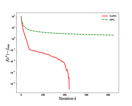
(a) $(m,n,\mbox{Spar})=(300,600,30\%)$.

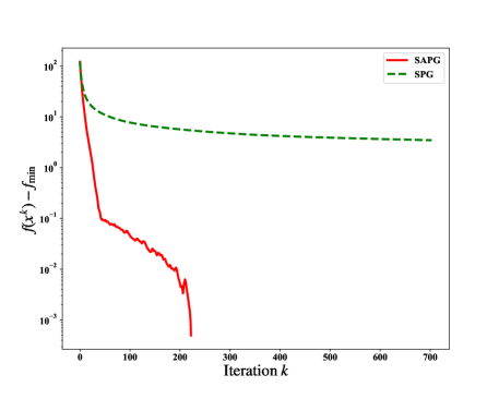
(b) $(m,n,\mbox{Spar})=(300,600,50\%)$.

Figure 4.1: Convergence of $\{f(x^{k})-f_{\min}\}$ for Example 4.1 with $m=300$, $n=600$ and different sparsity levels.

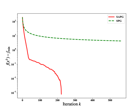
(a) $(m,n,\mbox{Spar})=(600,1200,30\%)$.

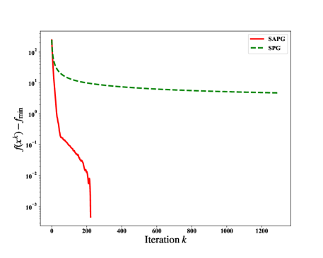
(b) $(m,n,\mbox{Spar})=(600,1200,50\%)$.

Figure 4.2: Convergence of $\{f(x^{k})-f_{\min}\}$ for Example 4.1 with $m=600$, $n=1200$ and different sparsity levels.

Example 4.2

We consider the following $\ell_{1}$ penalized censored regression problem:

$$\min_{\mathbf{0}\leq x\leq\mathbf{1}}\|\max\{Ax,0\}-b\|_{1}+0.01\|x\|_{1},$$ (72)

where the loss function is defined in (7) with $q=1$. For a given group of $(m,n,\mbox{Spar})$, the data in this example is generated as follows:

$B=\mbox{np.random.randn}(m,n);\ A=\mbox{orth}(B\mbox{.T})\mbox{.T};\ s=\mbox{Spar}*n;$

$x^{\star}=\mbox{np.random.uniform}(0,1,(n,1));\ x^{\star}[:n-s]=0;\ \mbox{np.random.shuffle}(x^{\star});$

$\bar{b}=A\mbox{.dot}(x^{\star});\ \mbox{per}=0.01\ast\mbox{np.random.rand}(\bar{b}\mbox{.shape}[0],\bar{b}\mbox{.shape}[1]);$

$b=\mbox{np.maximum}(\bar{b}+\mbox{per},\mbox{np.zeros}(\bar{b}\mbox{.shape})).$

A smoothing function of the loss function in (72) satisfying Definition 2.1 can be defined by Chen-MP

$$\begin{aligned} \tilde{f}(x,\mu)=\sum_{i=1}^{m}\tilde{\theta}(\tilde{\phi}(A_{i}x,\mu)-b_{i},\mu)\end{aligned}\quad\mbox{with}\quad\tilde{\phi}(z,\mu)=\left\{\begin{aligned} &\max\{z,0\}&\mbox{if}~{}|z|>\mu,\\ &\frac{(z+\mu)^{2}}{4\mu}&\mbox{if}~{}|z|\leq\mu.\end{aligned}\right.$$

For each fixed $(m,n,\mbox{Spar})$, we also randomly and independently generate 50 sets of data. In Table 2, we report the average values of iterations and CPU time for these 50 independent tests. We can see that the SAPG algorithm also performs better for problem (72) than the SPG algorithm in the sense that the SAPG algorithm needs less iterations and CPU time. From the comparisons between the SAPG algorithm and SPG algorithm in Figure 4.3 and Figure 4.4, we can also observe that the SAPG algorithm significantly outperforms the SPG algorithm in terms of convergence rate when solving problem (72) with different dimensions and sparsity levels.

Table 2: The average computational cost for Example 4.2 with different $m$, $n$ and Spar.

Methods		SAPG	SPG	SAPG	SPG	SAPG	SPG	SAPG	SPG
		$(1000,200)$		$(2000,400)$		$(4000,800)$		$(8000,1600)$
$20\%$	Iter	$\mathbf{223}$	250	$\mathbf{223}$	269	$\mathbf{223}$	248	$\mathbf{223}$	289
	Time	$\mathbf{0.0599}$	0.0674	$\mathbf{0.1268}$	0.1558	$\mathbf{0.2608}$	0.3052	$\mathbf{1.7238}$	2.3139
$30\%$	Iter	$\mathbf{223}$	434	$\mathbf{223}$	433	$\mathbf{223}$	451	$\mathbf{223}$	576
	Time	$\mathbf{0.0607}$	0.1150	$\mathbf{0.1266}$	0.2497	$\mathbf{0.2617}$	0.5598	$\mathbf{1.7295}$	4.6168
$40\%$	Iter	$\mathbf{223}$	502	$\mathbf{223}$	787	$\mathbf{223}$	917	$\mathbf{223}$	1162
	Time	$\mathbf{0.0591}$	0.1297	$\mathbf{0.1301}$	0.4542	$\mathbf{0.2752}$	1.2490	$\mathbf{1.7386}$	9.4325
$50\%$	Iter	$\mathbf{223}$	1034	$\mathbf{223}$	1236	$\mathbf{223}$	1819	$\mathbf{223}$	2327
	Time	$\mathbf{0.0615}$	0.2661	$\mathbf{0.1246}$	0.6788	$\mathbf{0.2640}$	2.4045	$\mathbf{1.7240}$	18.4405

(a) $(m,n,\mbox{Spar})=(2000,400,30\%)$.

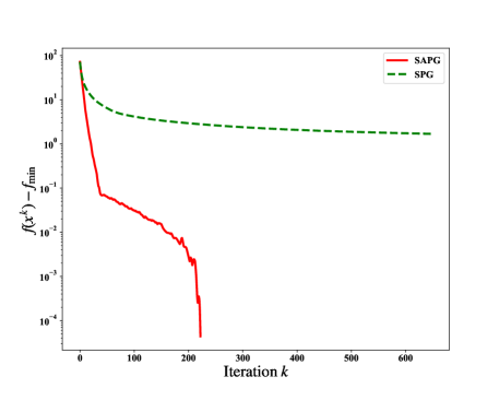
(b) $(m,n,\mbox{Spar})=(2000,400,50\%)$.

Figure 4.3: Convergence of $\{f(x^{k})-f_{\min}\}$ for Example 4.2 with $m=2000$, $n=400$ and different sparsity levels.

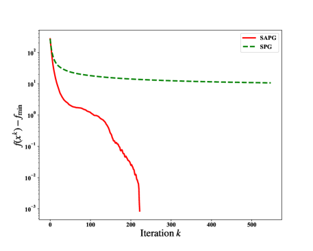
(a) $(m,n,\mbox{Spar})=(8000,1600,30\%)$.

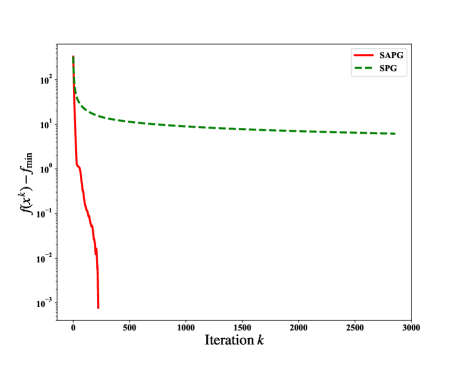
(b) $(m,n,\mbox{Spar})=(8000,1600,50\%)$.

Figure 4.4: Convergence of $\{f(x^{k})-f_{\min}\}$ for Example 4.2 with $m=8000$, $n=1600$ and different sparsity levels.

From the numerical results in Example 4.1 and Example 4.2, besides the faster convergence rate of the SAPG algorithm than the SPG algorithm, we have the following two observations.

• From Tables 1-2, we can see that the iteration numbers and CPU time of the SAPG algorithm are stable for all cases, while they are increasing as the sparsity is increasing for the SPG algorithm. This indicates that the superiority of the SAPG algorithm is highlighted when the sparsity level is large. It is surprising that the iteration number is 223 for all cases. We would like explain that the reason is that the value of $\|x^{k}-P_{\mathcal{X}}(x^{k}-\zeta\nabla\tilde{f}(x^{k},\mu_{k}))\|_{\infty}$ generated by the SAPG algorithm decreases rapidly, and the main work of the latter iterations is to update the smoothing parameter $\mu_{k}$ such that $\mu_{k}\leq\epsilon$ and the updating method for $\mu_{k}$ is same for all cases of Example 4.1 and Example 4.2.

• From Figures 4.1-4.4, the objective function values of the iterate obtained by SAPG algorithm are much smaller than those by the SPG algorithm, which shows that the SAPG algorithm can find a better $\epsilon$ minimizer with fewer iterations.

5 Conclusions

In this paper we develop a novel efficient smoothing accelerated proximal gradient (SAPG) algorithm for solving the constrained nonsmooth convex optimization problem modeled by (1), where the objective function is the sum of a continuous convex function (not necessarily smooth) and a proper closed convex function. The update method of the smoothing parameter is the essential for the convergence properties of the proposed algorithm. At each iteration, we employ the accelerated proximal gradient with extrapolation coefficient $\frac{k-1}{k+\alpha-1}$ to minimize problem (10) with a fixed smoothing parameter. We prove that the global convergence rate of the objective function values is $o(\ln^{\sigma}k/k)$ with any $\sigma\in(\frac{1}{2},1]$. In addition, we show that sequence $\{x^{k}\}$ converges to an optimal solution of problem (1). Further, we propose an inexact smoothing accelerated proximal gradient (ISAPG) algorithm by introducing an error or perturbation term in the SAPG algorithm. We obtain the fact that the convergence results of the ISAPG algorithm with appropriate perturbations are parallel to that of the SAPG algorithm.

- (1) Adly, S., Attouch, H.: Finite convergence of proximal-gradient inertial algorithms combining dry friction with Hessian-driven damping. SIAM Journal on Optimization 30(3), 2134–2162 (2020)
- (2) Attouch, H., Cabot, A.: Convergence rate of a relaxed inertial proximal algorithm for convex minimization. Optimization 69(6), 1281–1312 (2020)
- (3) Attouch, H., Chbani, Z., Fadili, J., Riahi, H.: First-order optimization algorithms via inertial systems with Hessian driven damping. Mathematical Programming (2020). DOI :10.1007/s10107-020-01591-1
- (4) Attouch, H., Chbani, Z., Peypouquet, J., Redont, P.: Fast convergence of inertial dynamics and algorithms with asymptotic vanishing viscosity. Mathematical Programming 168(1-2), 123–175 (2018)
- (5) Attouch, H., Chbani, Z., Riahi, H.: Fast proximal methods via time scaling of damped inertial dynamics. SIAM Journal on Optimization 29(3), 2227–2256 (2019)
- (6) Attouch, H., Chbani, Z., Riahi, H.: Convergence rate of inertial proximal algorithms with general extrapolation and proximal coefficients. Vietnam Journal of Mathematics 48(2), 247–276 (2020)
- (7) Attouch, H., Peypouquet, J.: The rate of convergence of Nesterov’s accelerated forward-backward method is actually faster than . SIAM Journal on Optimization 26(3), 1824–1834 (2016)
- (8) Aujol, J.F., Dossal, C.: Stability of over-relaxations for the forward-backward algorithm, application to FISTA. SIAM Journal on Optimization 25(4), 2408–2433 (2015)
- (9) Bauschke, H.H., Bolte, J., Teboulle, M.: A descent Lemma beyond Lipschitz gradient continuity: first-order methods revisited and applications. Mathematics of Operations Research 42(2), 330–348 (2017)
- (10) Beck, A., Hallak, N.: Proximal mapping for symmetric penalty and sparsity. SIAM Journal on Optimization 28(1), 496–527 (2018)
- (11) Beck, A., Hallak, N.: Optimization problems involving group sparsity terms. Mathematical Programming 178(1-2), 39–67 (2019)
- (12) Beck, A., Teboulle, M.: A fast iterative shrinkage-thresholding algorithm for linear inverse problems. SIAM Journal on Imaging Sciences 2(1), 183–202 (2009)
- (13) Bian, W.: Smoothing accelerated algorithm for constrained nonsmooth convex optimization problems (in Chinese). Scientia Sinica Mathematica 50(12), 1651–1666 (2020)
- (14) Bian, W., Chen, X.: A smoothing proximal gradient algorithm for nonsmooth convex regression with cardinality penalty. SIAM Journal on Numerical Analysis 58(1), 858–883 (2020)
- (15) Boyd, S., Parikh, N., Chu, E., Peleato, B., Eckstein, J.: Distributed optimization and statistical learning via the alternating direction method of multipliers. Foundations and Trends in Machine Learning 3(1), 1–122 (2011)
- (16) Bruck Jr, R.E.: Asymptotic convergence of nonlinear contraction semigroups in Hilbert spaces. Journal of Functional Analysis 18(1), 15–26 (1975)
- (17) Bruck Jr, R.E.: On the weak convergence of an ergodic iteration for the solution of variational inequalities for monotone operators in Hilbert space. Journal of Mathematical Analysis and Applications 61(1), 159–164 (1977)
- (18) Candès, E.J., Romberg, J., Tao, T.: Robust uncertainty principles: Exact signal reconstruction from highly incomplete frequency information. IEEE Transactions on Information Theory 52(2), 489–509 (2006)
- (19) Chambolle, A.: An algorithm for total variation minimization and applications. Journal of Mathematical Imaging and Vision 20(1-2), 89–97 (2004)
- (20) Chambolle, A., Dossal, C.: On the convergence of the iterates of the “fast iterative shrinkage/thresholding algorithm”. Journal of Optimization Theory and Applications 166(3), 968–982 (2015)
- (21) Chen, X.: Smoothing methods for nonsmooth, nonconvex minimization. Mathematical Programming 134(1), 71–99 (2012)
- (22) Chen, X., Kelley, C.T., Xu, F., Zhang, Z.: A smoothing direct search method for Monte Carlo-based bound constrained composite nonsmooth optimization. SIAM Journal on Scientific Computing 40(4), A2174–A2199 (2018)
- (23) Clarke, F.H.: Optimization and Nonsmooth analysis. Springer Science & Business Media (2009)
- (24) Donoho, D.L.: Compressed sensing. IEEE Transactions on Information Theory 52(4), 1289–1306 (2006)
- (25) Facchinei, F., Pang, J.S.: Finite-dimensional variational inequalities and complementarity problems. Springer Science & Business Media (2007)
- (26) Fan, J., Li, R.: Variable selection via nonconcave penalized likelihood and its oracle properties. Journal of the American Statistical Association 96(456), 1348–1360 (2001)
- (27) Fan, J., Xue, L., Zou, H.: Strong oracle optimality of folded concave penalized estimation. Annals of Statistics 42(3), 819 (2014)
- (28) Fukushima, M., Mine, H.: A generalized proximal point algorithm for certain non-convex minimization problems. International Journal of Systems Science 12(8), 989–1000 (1981)
- (29) Hoda, S., Gilpin, A., Pena, J., Sandholm, T.: Smoothing techniques for computing Nash equilibria of sequential games. Mathematics of Operations Research 35(2), 494–512 (2010)
- (30) Hong, M., Luo, Z.Q.: On the linear convergence of the alternating direction method of multipliers. Mathematical Programming 162(1-2), 165–199 (2017)
- (31) Koenker, R., Hallock, K.F.: Quantile regression. Journal of Economic Perspectives 15(4), 143–156 (2001)
- (32) Liu, Y., Ma, S., Dai, Y., Zhang, S.: A smoothing SQP framework for a class of composite minimization over polyhedron. Mathematical Programming 158(1-2), 467–500 (2016)
- (33) Lu, Z.: Iterative hard thresholding methods for regularized convex cone programming. Mathematical Programming 147(1-2), 125–154 (2014)
- (34) Nesterov, Y.: A method for solving the convex programming problem with the convergence rate . Doklady Akademii Nauk 269, 543–547 (1983)
- (35) Nesterov, Y.: Smooth minimization of non-smooth functions. Mathematical Programming 103(1), 127–152 (2005)
- (36) Nocedal, J., Wright, S.: Numerical optimization. Springer Science & Business Media (2006)
- (37) Opial, Z.: Weak convergence of the sequence of successive approximations for nonexpansive mappings. Bulletin of the American Mathematical Society 73(4), 591–597 (1967)
- (38) Parikh, N., Boyd, S.: Proximal algorithms. Foundations and Trends in Optimization 1(3), 123–231 (2013)
- (39) Passty, G.B.: Ergodic convergence to a zero of the sum of monotone operators in Hilbert space. Journal of Mathematical Analysis and Applications 72(2), 383–390 (1979)
- (40) Rockafellar, R.T., Wets, R.J.B.: Variational analysis. Springer Science & Business Media (2009)
- (41) Urruty, J.B.H., Lemaréchal, C.: Convex analysis and minimization algorithms. Springer-Verlag (1996)
- (42) Van Nguyen, Q.: Forward-backward splitting with Bregman distances. Vietnam Journal of Mathematics 45(3), 519–539 (2017)
- (43) Villa, S., Salzo, S., Baldassarre, L., Verri, A.: Accelerated and inexact forward-backward algorithms. SIAM Journal on Optimization 23(3), 1607–1633 (2013)
- (44) Xu, M., Ye, J.J., Zhang, L.: Smoothing SQP methods for solving degenerate nonsmooth constrained optimization problems with applications to bilevel programs. SIAM Journal on Optimization 25(3), 1388–1410 (2015)
- (45) Xue, X., Bian, W.: Subgradient-based neural networks for nonsmooth convex optimization problems. IEEE Transactions on Circuits and Systems I: Regular Papers 55(8), 2378–2391 (2008)
- (46) Yang, W.H., Han, D.R.: Linear convergence of the alternating direction method of multipliers for a class of convex optimization problems. SIAM Journal on Numerical Analysis 54(2), 625–640 (2016)
- (47) Zhang, C., Chen, X.: Smoothing projected gradient method and its application to stochastic linear complementarity problems. SIAM Journal on Optimization 20(2), 627–649 (2009)
- (48) Zhang, C., Chen, X.: A smoothing active set method for linearly constrained non-Lipschitz nonconvex optimization. SIAM Journal on Optimization 30(1), 1–30 (2020)