Instrumental Variable-Driven Domain Generalization with Unobserved Confounders

Abstract.

Domain generalization (DG) aims to learn from multiple source domains a model that can generalize well on unseen target domains. Existing DG methods mainly learn the representations with invariant marginal distribution of the input features, however, the invariance of the conditional distribution of the labels given the input features is more essential for unknown domain prediction. Meanwhile, the existing of unobserved confounders which affect the input features and labels simultaneously cause spurious correlation and hinder the learning of the invariant relationship contained in the conditional distribution. Interestingly, with a causal view on the data generating process, we find that the input features of one domain are valid instrumental variables for other domains. Inspired by this finding, we propose an instrumental variable-driven DG method (IV-DG) by removing the bias of the unobserved confounders with two-stage learning. In the first stage, it learns the conditional distribution of the input features of one domain given input features of another domain. In the second stage, it estimates the relationship by predicting labels with the learned conditional distribution. Theoretical analyses and simulation experiments show that it accurately captures the invariant relationship. Extensive experiments on real-world datasets demonstrate that IV-DG method yields state-of-the-art results.

1. Introduction

General supervised learning extracts statistical patterns by assuming data across training (source) and test (target) sets are independent and identically distributed (i.i.d.). It may lead to poor generalization performance when testing the trained model on the data that is very distinct from the training one, which is known as the dataset shift (or domain shift) problem (Quionero-Candela et al., 2009). A prevailing research field for addressing this problem is domain adaptation (DA) (Ben-David et al., 2010), which adapts the model from source to target with available target data. However, DA methods need to re-collect target data and repeat the model adaptation process for each new target domain, which is time-consuming or even infeasible. Domain generalization (DG) (Blanchard et al., 2011) is thus proposed to use multiple semantically-related source datasets for learning a generalizable model without accessing any target data/information.

Numerous DG works (Li et al., 2018c; Matsuura and Harada, 2020; Peng et al., 2019; Zhao et al., 2020) learn domain-agnostic feature representations. Most of them (Li et al., 2018c; Matsuura and Harada, 2020; Peng et al., 2019) are based on the covariate shift assumption that the marginal distribution of the input features, i.e., $P(X)$, changes yet the conditional distribution of the labels given the input features, i.e., $P(Y|X)$, stays unchanged across domains. However, it rarely holds in many real scenarios where $P(Y|X)$ also changes in different domains/environments. Since the goal of DG is to improve the generalization performance of the prediction $P(Y|X)$ on unseen target domains, it is essential to capture the invariance of $P(Y|X)$ that could be extracted from the source domains. But there might exist unobserved confounders that affect $X$ and $Y$ simultaneously. They cause spurious correlation between $X$ and $Y$, hindering the learning of the invariant relationship contained in $P(Y|X)$.

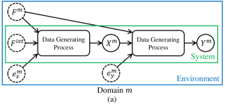
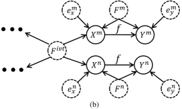
Figure 1. (a): A causal view on the data generating process for each domain $m$. (b): a causal graph for different domains. Solid and dashed circles denote observed and latent variables, respectively. For each domain $m$, input features $X^{m}$ and labels $Y^{m}$ are (indirectly) determined by domain-invariant factor $F^{ivt}$ of the system, confounded by domain-specific factor $F^{m}$ (unobserved confounder), and affected by error $e_{x}^{m}$ and $e_{y}^{m}$ from the environment. We aim to learn the invariant relationship $f$ between the input features and the labels with an instrumental variable-based method for improving the out-of-distribution generalization performance.

In this paper, we aim to capture the invariant relationship between the input features and the labels by removing the bias of the unobserved confounders for robust domain generalization. We tackle this issue by putting forward a causal view on the data generating process which distinguishes domain-invariant and domain-specific parts of data as shown in Figure 1 (a). In an analyzed system of domain $m$, input features $X^{m}$ and labels $Y^{m}$ are (indirectly) determined by domain-invariant factor $F^{ivt}$ that contains discriminative semantic information of objects. The domain-specific factor $F^{m}$ plays the role of a common cause of $X^{m}$ and $Y^{m}$ by affecting both of them. $X^{m}$ and $Y^{m}$ are also affected by error $e_{x}^{m}$ and $e_{y}^{m}$ from the environment of domain $m$. In light of this, we build a causal graph of different domains in Figure 1 (b). We attribute the changes of the conditional distribution $P(Y|X)$ across domains to the changes of the unobserved confounder, i.e., the domain-specific factor $F^{m}$ here. Moreover, we assume that there exists an invariant relationship $f$ between the input features and the labels, contained in $P(Y|X)$, which we are interested in. With the analysis of Figure 1, we find that the input features of one domain are valid instrumental variables (IVs) (Wright, 1928) (see Section 3) of another domain. Inspired by this finding, we propose an Instrumental Variable-driven DG method (IV-DG) to learn the relationship $f$ with two-stage learning. It first learns the conditional distribution of the input features of one domain given the input features of another domain, and then estimates $f$ by predicting the labels with the learned conditional distribution. Our method is simple yet effective that helps the model remove the bias of the unobserved confounder and learn the invariant relationship, effectively improving the generalization performance of the model. We demonstrate with theoretical analyses to verify the effectiveness of our method. Extensive experiments on both simulated and real-world data show its superior performance.

Our main contributions are summarized as follow: (i) We formulate a data generating process by distinguishing domain-invariant and domain-specific parts in data. Based on this, we build a causal graph of different domains to analyze the problem of the unobserved confounders in the domain generalization task from a causal perspective. (ii) We propose an Instrumental Variable-driven Domain Generalization (IV-DG) method to learn the domain-invariant relationship for improving model generalization. It exploits the input features of one domain as IVs for another domain and implements IV-based generalization learning by removing the bias of the unobserved confounders. (iii) We provide theoretical analyses to verify our method. Moreover, extensive experiments on both simulated data and real-world datasets show that our method yields state-of-the-art results.

The remainder of this paper is organized as follows. Section 2 gives a brief review of the related works on domain adaptation, domain generalization, and instrumental variables. The formulation of the investigated domain generalization problem and preliminary of instrumental variables are introduced in Section 3. The proposed method is presented in Section 4. The experiments on simulated and real-world data and analysis are demonstrated in Section 5. Finally, Section 6 concludes this paper, with a future research outlook.

2. Related Work

2.1. Domain Adaptation and Generalization

Domain adaptation (DA) (Chattopadhyay et al., 2012; Wu and Ng, 2022; Zhou et al., 2020a; Cai et al., 2019; Ren et al., 2020; Ma et al., 2021, 2022; Zhang et al., 2019a; Long et al., 2015) aims to transfer the knowledge from the source domain(s) to the target domain(s). Unsupervised domain adaptation (Cai et al., 2019; Ma et al., 2021; Zhang et al., 2019a; Long et al., 2015) is a prevailing direction to DA that addresses the domain shift problem by minimizing domain gap between a labeled source domain and an unlabeled target domain via domain adversarial learning (Cai et al., 2019; Ma et al., 2021) or domain distance minimization (Zhang et al., 2019a; Long et al., 2015), et al. However, they need to access the data/information of the target domain in advance, which may be expensive or even infeasible in real scenarios.

Domain generalization (DG) (Zhou et al., 2021; Yuan et al., 2023b; Lv et al., 2023b, a; Shankar et al., 2018; Volpi et al., 2018; Lv et al., 2022; Niu et al., 2023; Yuan et al., 2023a, 2022a) is proposed to use multiple labeled source domains for training a generalizable model to unseen target domains. Recent DG methods with a variety of strategies can be included in the following main topics. The first topic is domain-invariant representation learning. This line of works learns feature representations that are invariant to domains and discriminative for classification. Some works (Ghifary et al., 2015; Li et al., 2018b; Qiao et al., 2020) use auto-encoder structure to obtain invariant representations by performing a data reconstruction task. Li et al. (Li et al., 2018a) learn invariant class conditional representation with kernel mean embeddings. Piratla et al. (Piratla et al., 2020) decompose networks into common and specific components, making the model rely on the common features. Li et al. (Li et al., 2018c; Matsuura and Harada, 2020) introduce adversarial learning to extract effective representations with invariance constraints. Zhao et al. (Zhao et al., 2020) introduce conditional entropy regularization term to learn conditional invariant features. Li et al. (Li et al., 2020) model linear dependency in feature space and learn the common information. Data augmentation-based methods aim to boost generalization ability of the model by training it on various generated novel domains. Some methods (Shankar et al., 2018; Volpi et al., 2018) use model gradient to perturb data and construct new datasets for model training. Some others (Carlucci et al., 2019; Wang et al., 2020) augment datasets by solving jigsaw puzzles. Zhou et al. (Zhou et al., 2020b, c) employ an adversarial strategy to generate novel domains while keeping semantic information consistent. A recent work (Zhou et al., 2021) mixes instance features to synthesize diverse domains and improves generalization. Similar to the goal of DG, meta-learning-based methods keeps training the model on a meta-train dataset and improving its performance on a meta-test dataset. Numerous works (Balaji et al., 2018; Li et al., 2018d; Dou et al., 2019; Li et al., 2019b, a) put forward meta-learning guided training algorithms to improve model out-of-domain generalization. However, it may be difficult to design effective yet efficient meta-learning training algorithms in practice. Some other methods learn the masks of features (Chattopadhyay et al., 2020) or gradient (Huang et al., 2020) for regularization, or normalize batch/instance (Seo et al., 2020).

2.2. Causality-based Distribution Generalization

To learn distribution-irrelevant features and models for stable generalization, numerous causality-based distribution generalization methods (Mahajan et al., 2021; Yang et al., 2021; Zhang et al., 2013, 2015; Kuang et al., 2020; Fan et al., 2020; Miao et al., 2022; Christiansen et al., 2021; Gong et al., 2016; Wu et al., 2022; Yuan et al., 2022b) have been introduced recently. For example, Yang et al. (Yang et al., 2021) investigate a robust domain adaptation problem where only a source dataset is available. They design a causal autoencoder to learn causal representations via causal structure learning. Mahajan et al. (Mahajan et al., 2021) provide a causal interpretation of domain generalization, and show the importance of learning within-class variations for generalization. Lu et al. (Lu et al., 2022) and Wang et al. (Wang et al., 2021) also propose to learn domain-agnostic features for out-of-distribution generalization through knowledge distillation and variational disentanglement, respectively. Another direction is causal feature selection (Lin et al., 2022a, b; Mao et al., 2022, 2021). For example, Mao et al. (Mao et al., 2021) propose to steer generative model to manufacture interventions on confounded features for learning robust visual representations.

Compared to the previous works, our work has the following merits. (i) We provide a causal view on the data generating process for domain generalization with unobserved confounders. We then find that the input features can be treated as Instrumental Variables (IVs) for another domains. This finding inspires us to use the IVs to remove the domain-specific factors and capture the invariant relationship between the input features and labels. This idea of IVs for causality-based generalization learning is seldomly investigated to our knowledge, and we believe our work would shed lights on this interesting direction. (ii) To verify this idea, we further provide theoretical insights and toy experiments which shows that the relationship estimated by our method converges to the causal invariant relationship. (iii) We propose a model-agnostic learning framework for the domain generalization task, which can easily deal with high-dimensional non-linear data. We implement simulation experiments on both linear and non-linear data to show the invariance learning ability of our method. Furthermore, we perform experiments on four real-world data to show the great generalization learning performance of our method. However, previous methods may either perform experiments on low-dimensional toy data (Zhang et al., 2013; Gong et al., 2016; Christiansen et al., 2021) or lack simulation results to show its causality learning performance (Mahajan et al., 2021; Yang et al., 2021).

2.3. Instrumental Variable

Instrumental variable (IV) method (Wright, 1928) is widely employed to capture causal relationship between variables for counterfactual prediction. Two stage least squares (2SLS) (Angrist and Pischke, 2008) is the most prevailing method in IV-based counterfactual prediction, which learns $\mathbb{E}[\phi(X)|Z]$ with IV $Z$ and linear basis $\phi(\cdot)$, and fits $Y$ by least squares regression with the coefficient $\hat{\phi}(\cdot)$ estimated in the first stage. Some non-parametric researches (Newey and Powell, 2003) extend the model basis to more complicated mapping function or regularization, e.g., polynomial basis. DeepIV (Hartford et al., 2017) is proposed to use deep neural networks in the two-stage procedure, it fits a mixture density network $F_{\phi}(X|Z)$ in the first stage and regresses $Y$ by sampling from the estimated mixture Gaussian distributions of $X$. KIV (Singh et al., 2019) is a recent work which maps and learns the relationships among $Z$, $X$, and $Y$ in reproducing kernel Hilbert spaces. Another recent progress, DeepGMM (Bennett et al., 2019), extends GMM methods in high-dimensional treatment and IV settings based on variational reformulation of the optimally-weighted GMM. We follow the additive function form used by most of the previous IV-based methods, i.e., $Y=f(X)+e$.

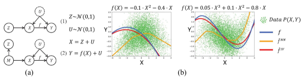
Figure 2. (a): two examples (Pearl, 2009) of causal structure with an instrumental variable (IV) $Z$, covariates (or input features) $X$, response (or output) $Y$, unobserved confounder $U$, and intermediate variable $M$. (b): toy experiments where $\hat{f}^{NN}$ and $\hat{f}^{IV}$ are estimated by neural networks (NN) and instrumental variable (IV) methods, respectively, on the data sampled from the biased distribution $P(X,Y)$. $\hat{f}^{NN}$ is estimated by directly taking $X$ and $Y$ as the model input and target, respectively, for training. $\hat{f}^{IV}$ is estimated via an IV-based two-stage method with IV $Z$. We utilize the IV $Z$ to estimate the invariant relationship $f$ between $X$ and $Y$ by removing the confounding effect of an unobserved confounder $U$ in the biased distribution $P(X,Y)$.

3. Preliminary

In the domain generalization (DG) task, we have $Q$ labeled source datasets $\mathcal{D}_{1},...,\mathcal{D}_{Q}$ with different distributions $P_{1}(X^{1},Y^{1}),...,P_{Q}(X^{Q},Y^{Q})$ on joint space $\mathcal{X}\times\mathcal{Y}$, where $\mathcal{X}$ and $\mathcal{Y}$ are input feature and label spaces, respectively. In each source domain $q$, $N^{q}$ examples are sampled for the dataset $\mathcal{D}_{q}$, i.e., $\mathcal{D}_{q}=\{(\mathrm{x}_{n}^{q},y_{n}^{q})\}_{n=1}^{N^{q}}$. Despite the distribution shift across domains, the input features $X^{q}$ as well as the labels $Y^{q}$ represent the same object and used for the same task across domains. DG aims to train a model with the $Q$ source datasets and improve its generalization performance on the unseen target domains where no data or information is provided for training.

In causal literature (Pearl, 2009), invariant relationship (response function) $f$ between covariates $X$ and response $Y$ is assumed as shown in Figure 2 (a). The unobserved confounder $U$, which causes changes to both $X$ and $Y$, introduces bias in data distribution $P(X,Y)$. The estimation of the relationship $P(Y|X)$ by learning from $P(X,Y)$ hence varies across domains with the changes of $U$. Instrumental variable (IV) (Wright, 1928) $Z$ is a powerful tool for tracking the bias from the unobserved confounder $U$. A valid IV should satisfy the following conditions (Pearl, 2009; Hartford et al., 2017): (i) Relevance. $Z$ and $X$ should be relevant, i.e., $P(X|Z)\neq{P(X)}$; (ii) Exclusion. $Z$ is correlated to $Y$ only through $X$, i.e., $Z\upmodels Y|(X,U)$; and (iii) Unconfounded instrument. $Z$ is independent of $U$, i.e., $Z\upmodels U$. These conditions make $Z$ a valid IV, which allows us to learn the true relationship $f$ between $X$ and $Y$ by considering the changes of $Z$. Instead of directly leveraging $X$ to predict $Y$ for capturing relationship between $X$ and $Y$ in supervised learning, the general procedure of two-stage IV method is to learn the distribution of $X$ given $Z$ and then use the estimated conditional distribution to predict $Y$.

We compare the functions estimated by direct neural networks (NN), i.e., general supervised learning, and IV method by conducting toy experiments with 4000 data points sampled for training and test, respectively. The results are shown in Figure 2 (b). We see that NN (orange line) directly learns $P(X,Y)$ that is biased by $U$, while IV method (red line) uses $Z$ to eliminate the bias from $U$ and estimates $f$ (blue line), i.e. the invariant causal relationship, more accurately.

For theoretical analysis, we consider a simple linear model

(1) $$\mathbf{Y}=\mathbf{X}\cdot\lambda+\mathbf{U},$$

where $\mathbf{Y},\mathbf{U}\in\mathbb{R}^{n}$, $\mathbf{X}\in\mathbb{R}^{n\times d_{x}}$, $\lambda\in\mathbb{R}^{d_{x}}$, $n$ and $d_{x}$ are the number of observations and dimension of $X$, respectively. The invariant relationship $f$ is assumed as a linear mapping vector $\lambda$. We estimate $\lambda$ via a two-stage IV method ($\hat{\lambda}^{IV}$) and an ordinary least squares (OLS) method ($\hat{\lambda}^{OLS}$). We have

$$\hat{\lambda}^{OLS}= ((\mathbf{X})^{\top}\mathbf{X})^{-1}(\mathbf{X})^{\top}\mathbf{Y}$$

$$= ((\mathbf{X})^{\top}\mathbf{X})^{-1}(\mathbf{X})^{\top}(\mathbf{X}\cdot\lambda+\mathbf{U})$$

$$= \lambda+\underbrace{((\mathbf{X})^{\top}\mathbf{X})^{-1}(\mathbf{X})^{\top}\mathbf{U}}_{\text{ not converges to 0 for $X$ is correlated with $U$ }},$$

$$\hat{\lambda}^{IV}= ((\mathbf{Z})^{\top}\mathbf{X})^{-1}(\mathbf{Z})^{\top}\mathbf{Y}$$

$$= ((\mathbf{Z})^{\top}\mathbf{X})^{-1}(\mathbf{Z})^{\top}(\mathbf{X}\cdot\lambda+\mathbf{U})$$

$$= \lambda+\underbrace{((\mathbf{Z})^{\top}\mathbf{X})^{-1}(\mathbf{Z})^{\top}\mathbf{U}}_{\text{ converges to 0 for $Z$ is independent of $U$ }}.$$

The IV method utilizes $Z$ to eliminate the bias of $U$ and the estimator $\hat{\lambda}^{IV}$ converges to $\lambda$; but the OLS estimator is biased. In light of this, we aim to design IV-based algorithm to capture invariant relationship between input features and labels across domains and improve the generalization performance of the trained model on unknown target domains.

4. Instrumental Variable-Driven Generalization Learning

We begin by giving a causal view on domain generalization. Based on it, we introduce our method, i.e., Instrumental Variable-driven Domain Generalization (IV-DG), followed by theoretical analyses. We finally demonstrate the detailed framework and algorithm of the proposed method.

4.1. A Causal View on Domain Generalization

The general supervised learning imposes an i.i.d. assumption, however, changes in the external environment of a new domain will lead to changes in the analyzed system (i.e., variables and their relationships). The general supervised model trained on one domain may overfit the domain-specific information, leading to the degradation of the generalization ability of the model on a new domain where the external environment changes. Nevertheless, we see that human can easily identify relationship in data no matter how the environment changes, e.g., to recognize images of animals with different backgrounds. We argue that the robust perception of human is based on the ability to distinguish domain-invariant and domain-specific parts in data via causal reasoning (Zhang et al., 2020a). In light of this, it is necessary to analyze the dataset shift problem from a causal view by defining the latent data generating process (DGP) first.

Taking a visual recognition task of animals as an example. As shown in Figure 1 (a), $X^{m}$ and $Y^{m}$ are images and classes sampled from a specific dataset/domain $m$. There may exist multiple causes in the DGP of $X^{m}$ and $Y^{m}$. Inspired by (Zhang et al., 2020b), we argue that $X^{m}$ is determined by: (i) domain-invariant factor $F^{ivt}$, which is the key part of the recognized animals like size and limbs; (ii) domain-specific factor $F^{m}$ that changes with the external environment, like light condition and background when taking pictures; (iii) an error term $e_{x}^{m}$. In the DGP, the factor $F^{ivt}$ is invariant across domains, but the unobserved confounder $F^{m}$ plays the role of a common cause of $X^{m}$ and $Y^{m}$, leading to confounding bias and distribution shift across domains. For human, no matter how the images change, the corresponding classes can always be identified. It allows us to argue that there exists a latent domain-invariant relationship between input features $X^{m}$ and labels $Y^{m}$. Therefore, we let $Y^{m}$ be determined by $X^{m}$ that contains invariant information of $F^{ivt}$, and $Y^{m}$ is also affected by $F^{m}$ and $e_{y}^{m}$. Note that only the input features and labels are observed, and the others are unobserved.

Based on the DGP, we build a causal graph of different domains as shown in Figure 1 (b). Input features $X^{m}$/$X^{n}$ from domain $m$/$n$ shares domain-invariant factor $F^{ivt}$ and is affected by different domain-specific factor $F^{m}$/$F^{n}$ and error $e_{x}^{m}$/$e_{x}^{n}$. Label $Y^{m}$/$Y^{n}$ is determined by $X^{m}$/$X^{n}$ through the relationship $f$, and is influenced by $F^{m}$/$F^{n}$ and $e_{y}^{m}$/$e_{y}^{n}$.

Assumption 1.

Data distributions of different domains satisfy the data generating process and causal graph in Figure 1, where only the factor $F^{ivt}$ and relationship $f$ are invariant.

In each domain $m$, general supervised learning trains the model to learn conditional distribution:

(2) $$P(Y^{m}|X^{m})= \int{P(Y^{m}|X^{m},F^{m})P(F^{m}|X^{m})}dP(F^{m}).$$

The domain-specific factor $F^{m}$ is a common cause of $X^{m}$ and $Y^{m}$, leading to spurious correlation between $X^{m}$ and $Y^{m}$, hence the conditional distribution changes across domains. Since $F^{m}$ is latent and can not be controlled, the introduced bias in data may not be removed directly. The model trained by minimizing risk on one domain overfits the bias and may have terrible performance on a new domain where the spurious correlation is different with the changes of the domain-specific factor. Since directly minimizing the risk on target domains is impossible as the data is unknown, instead, we propose to learn the relationship $f$ between the input features and the labels which is invariant across domains. In causal literature (Pearl, 2009), utilizing instrumental variable (IV) is an effective way to address the spurious correlation from the unobserved factor. By finding that the input features of one domain are valid IVs for other domains, we propose an IV-based two-stage method to learn the relationship $f$ for stable domain generalization, which is introduced in the following.

4.2. Learning Domain-Invariant Relationship with Instrumental Variable

Under Assumption 1, we give the following conclusions by using d-separation criterion (Pearl, 2009).

Proposition 1.

For any two domains $m$ and $n$, if $m\neq{n}$, then the following conditions hold: (1) $X^{n}\nupmodels{X^{m}}$; (2) $X^{n}\upmodels{Y^{m}}|(X^{m},F^{m})$; (3) $X^{n}\upmodels{F^{m}}$; and (4) $X^{n}\upmodels{e_{y}^{m}}$.

Based on the above proposition, we have the following finding.

Theorem 1.

For any two domains $m$ and $n$, if $m\neq{n}$, then $X^{n}$ is a valid instrumental variable of domain $m$.

This theorem can be proved by referring to the conditions of IV in Section 3. It indicates that one may adopt the input features of one source dataset as valid IVs to estimate the domain-invariant relationship $f$ with another source dataset via a two-stage IV process (see Section 3). That is, we first estimate the conditional distribution $P(X^{m}|X^{n})$, and then predict labels $Y^{m}$ with $P(X^{m}|X^{n})$ instead of the input features $X^{m}$. Since $X^{n}$ is independent of $F^{m}$, the changes of $X^{n}$ through $X^{m}$ to $Y^{m}$ is stable to the changes of $F^{m}$. The estimation process can be understood as indirectly learning the changes of $X^{m}$ with the changes of $F^{ivt}$, i.e., parent of $X^{m}$ and $X^{n}$. $F^{ivt}$ determines the class of the analyzed system, hence the estimated relationship between $X^{m}$ and $Y^{m}$ via this two-stage procedure is discriminative for classification yet insensitive to domain changes. By following (Hartford et al., 2017; Singh et al., 2019; Bennett et al., 2019), we assume that the label $Y^{m}\in\mathbb{R}$ is structurally determined by the following DGP:

(3) $$Y^{m}=f(X^{m})+\alpha_{m}^{\top}F^{m}+e_{y}^{m},$$

where $f(\cdot)$ is an unknown continuous function, $\alpha_{m}\in\mathbb{R}^{d_{f}}$ is coefficient vector of $F^{m}\in\mathbb{R}^{d_{f}}$, $d_{f}$ is the dimension of factor, $\mathbb{E}[F^{m}]=\mathbf{0}$ and $\mathbb{E}[e_{y}^{m}]=0$. By taking the expectation of $Y^{m}$ conditional on $X^{n}$, we have:

(4) $$\mathbb{E}[Y^{m}|X^{n}]= \mathbb{E}[f(X^{m})|X^{n}]+\underbrace{\mathbb{E}[\alpha_{m}^{\top}F^{m}|X^{n}]+\mathbb{E}[e_{y}^{m}|X^{n}]}_{=0\text{ for }X^{n}\upmodels{F^{m}}\text{ and }X^{n}\upmodels{e_{y}^{m}}}$$

$$= \underbrace{\int{f(X^{m})\underbrace{dP(X^{m}|X^{n})}_{\text{stage 1}}}}_{\text{stage 2}}.$$

It yields a two-stage strategy of learning the invariant relationship $f$ with the instrumental variable $X^{n}$. That is, in the first stage, we estimate conditional distribution $P(X^{m}|X^{n})$; and in the second stage, we estimate the invariant relationship $f$ via the approximation of $P(X^{m}|X^{n})$ learned in the first stage, i.e., predict the label $Y^{m}$ with the estimated $P(X^{m}|X^{n})$.

We further consider a linear setting to make it clearer. Let the dimensions of the factors and input features be $d_{f}$ and $d_{x}$, respectively, i.e., $F^{ivt}\in\mathbb{R}^{d_{f}}$, $F^{m}\in\mathbb{R}^{d_{f}}$, $X^{m}\in\mathbb{R}^{d_{x}}$. Note that we assume $F^{ivt}$ and $F^{m}$ have the same dimension, because they could be the extracted features from data, as implemented in our framework. The error terms and label are real numbers, i.e., $e_{x}^{m}\in\mathbb{R}$, $e_{y}^{m}\in\mathbb{R}$, $Y^{m}\in\mathbb{R}$. Assume that we sample $n$ observations from each domain. We stack all observations together, i.e., let $\mathbf{X}^{m}$ be the matrix where $i$-th row is observation $(x_{i}^{m})^{\top}$. Other bold symbols are similarly defined. The DGP is then assumed as:

(5) $$\mathbf{X}^{m}= \begin{bmatrix}\mathbf{F}^{ivt}&\mathbf{F}^{m}\end{bmatrix}\begin{bmatrix}\boldsymbol{\phi}_{m}\\ \boldsymbol{\alpha}_{m}\end{bmatrix}+\mathbf{e}^{m}_{x}$$

$$\mathbf{Y}^{m}= \begin{bmatrix}\mathbf{X}^{m}&\mathbf{F}^{m}\end{bmatrix}\begin{bmatrix}\lambda_{ivt}\\ \beta_{m}\end{bmatrix}+\mathbf{e}^{m}_{y},$$

where $\boldsymbol{\phi}_{m}$, $\boldsymbol{\alpha}_{m}$, $\lambda_{ivt}$, and $\beta_{m}$ are coefficients. Note that $\lambda_{ivt}$ is the invariant relationship between input features and labels. Let input features $X^{n}$ from domain $n$, where $n\neq{m}$, be the IV for performing the two-stage IV method. The first stage is to learn the conditional distribution of $X^{m}$ by regressing $\mathbf{X}^{m}$ on the IV $\mathbf{X}^{n}$ with $\hat{\gamma}$, that is,

(6) $$\hat{\gamma}= \big{(}(\mathbf{X}^{n})^{\top}\mathbf{X}^{n}\big{)}^{-1}(\mathbf{X}^{n})^{\top}\mathbf{X}^{m}.$$

Then, the second stage is to predict label $\mathbf{Y}^{m}$ with the estimated conditional distribution, i.e., regressing $\mathbf{Y}^{m}$ on $\hat{\mathbf{X}}^{m}=\mathbf{X}^{n}\hat{\gamma}$ with estimated relationship $\hat{\lambda}_{ivt}^{IV}$, that is,

(7) $$\hat{\lambda}_{ivt}^{IV}= \big{(}(\hat{\mathbf{X}}^{m})^{\top}\hat{\mathbf{X}}^{m}\big{)}^{-1}(\hat{\mathbf{X}}^{m})^{\top}\mathbf{Y}^{m}.$$

Here, $\mathbf{Y}^{m}$, $\mathbf{X}^{m}$, and $\lambda_{ivt}$ in Eq. (5) correspond to $\mathbf{Y}$, $\mathbf{X}$, and $\lambda$ in Eq. (1), respectively. $\mathbf{F}^{m}\beta_{m}$ in Eq. (5) corresponds to the unobserved confounder $\mathbf{U}$ in Eq. (1). Different from the preliminary section that the IV $\mathbf{Z}$ is available, we consider a more practical scenario that only the input features and labels are available. Thus, we propose to utilize the input features of another domain, i.e., $\mathbf{X}^{n}$, as IV to perform the two-stage learning process introduced in the preliminary section.

Then, we have the following theorem.

Theorem 2.

Suppose the minimum eigenvalue of $\boldsymbol{\phi}_{m}^{\top}\cdot\mathbb{E}[F^{ivt}(F^{ivt})^{\top}]\cdot\boldsymbol{\phi}_{m}$ is bounded away from 0, and each variable of $F^{ivt}$, $F^{m}$, $e_{x}^{n}$, and $e_{y}^{n}$ of a random domain $m$ has a finite variance, then $\hat{\lambda}_{ivt}^{IV}$ is a consistent estimator which converges to $\lambda_{ivt}$, that is, $\hat{\lambda}_{ivt}^{IV}={\lambda}_{ivt}+O_{p}\left(\frac{1}{\sqrt{n}}\right)$.

Proof. Since $F^{m}$ is uncorrelated with $F^{ivt}$, $F^{n}$, and $e_{x}^{n}$ (d-separation), together with $\mathbb{E}[F^{m}]=\mathbf{0}$ and $\mathbb{E}[e^{n}_{x}]=0$, we have

(8) $$\frac{1}{n}(\mathbf{F}^{ivt})^{\top}\mathbf{F}^{m}=O_{p}\bigg{(}\frac{1}{\sqrt{n}}\bigg{)},$$

$$\frac{1}{n}(\mathbf{F}^{n})^{\top}\mathbf{F}^{m}=O_{p}\bigg{(}\frac{1}{\sqrt{n}}\bigg{)},$$

$$\frac{1}{n}(\mathbf{e}^{n}_{x})^{\top}\mathbf{F}^{m}=O_{p}\bigg{(}\frac{1}{\sqrt{n}}\bigg{)}.$$

Eq. (8) can be proved based on Central Limit Theorem (CLT) (Heyde, 2006). Specifically, we assume two uncorrelated variables $x_{a}$ and $x_{b}$ with zero means and finite variances, and let $x=x_{a}x_{b}$. Using CLT, we know that as the sample numbers $n$ becomes large, the distribution of $\sqrt{n}\bar{x}$ converges in distribution to a normal distribution with mean $0$ and variance $\sigma^{2}$, where $\sigma^{2}$ is the variance of $x$. That is, $\sqrt{n}\bar{x}\xrightarrow{d}\mathcal{N}(0,\sigma^{2})$, which can be rewritten to $\frac{\bar{x}}{\sqrt{\frac{\sigma^{2}}{n}}}\xrightarrow{d}\mathcal{N}(0,1)$. Since $\sigma^{2}$ is the variance of $x$, we have $\sqrt{\frac{\sigma^{2}}{n}}=\frac{\sigma}{\sqrt{n}}$. Then, $\frac{\bar{x}}{\sigma/\sqrt{n}}\xrightarrow{d}\mathcal{N}(0,1)$. This implies that $\frac{\bar{x}}{\sigma/\sqrt{n}}=O_{p}(1)$, which in turn implies that $\bar{x}=O_{p}(\frac{\sigma}{\sqrt{n}})$. Since $\sigma$ is a constant (dependent on the distribution of $x_{i}$), we have $\bar{x}=O_{p}(\frac{1}{\sqrt{n}})$. Hence, $1/n\sum_{i}x_{i}=\bar{x}=O_{p}(1/\sqrt{n})$. Therefore, Eq. (8) holds.

Then, we have

(9) $$\frac{1}{n}(\mathbf{X}^{n})^{\top}\mathbf{F}^{m}= \frac{1}{n}\big{(}\mathbf{F}^{ivt}\boldsymbol{\phi}_{n}+\mathbf{F}^{n}\boldsymbol{\alpha}_{n}+\mathbf{e}^{n}_{x}\big{)}^{\top}\mathbf{F}^{m}=O_{p}\bigg{(}\frac{1}{\sqrt{n}}\bigg{)}.$$

Similarly, since $e_{y}^{m}$ is independent of $F^{ivt}$, $F^{n}$, and $e_{x}^{n}$, then

(10) $$\frac{1}{n}(\mathbf{X}^{n})^{\top}\mathbf{e}_{y}^{m}= \frac{1}{n_{m}}\big{(}\mathbf{F}^{ivt}\boldsymbol{\phi}_{n}+\mathbf{F}^{n}\boldsymbol{\alpha}_{n}+\mathbf{e}^{n}_{x}\big{)}^{\top}\mathbf{e}_{y}^{m}=O_{p}\bigg{(}\frac{1}{\sqrt{n}}\bigg{)}.$$

We then have

(11) $$\frac{1}{n}(\mathbf{X}^{m})^{\top}\mathbf{X}^{n}= \frac{1}{n}\big{(}\mathbf{F}^{ivt}\boldsymbol{\phi}_{m}+\mathbf{F}^{m}\boldsymbol{\alpha}_{m}+\mathbf{e}^{m}_{x}\big{)}^{\top}$$

$$\cdot\big{(}\mathbf{F}^{ivt}\boldsymbol{\phi}_{n}+\mathbf{F}^{n}\boldsymbol{\alpha}_{n}+\mathbf{e}^{n}_{x}\big{)}$$

$$= \frac{1}{n}\boldsymbol{\phi}_{m}^{\top}(\mathbf{F}^{ivt})^{\top}\mathbf{F}^{ivt}\boldsymbol{\phi}_{n}+O_{p}\bigg{(}\frac{1}{\sqrt{n}}\bigg{)},$$

(12) $$\frac{1}{n}(\mathbf{X}^{n})^{\top}\mathbf{X}^{n}= \frac{1}{n}\big{(}\mathbf{F}^{ivt}\boldsymbol{\phi}_{n}+\mathbf{F}^{n}\boldsymbol{\alpha}_{n}+\mathbf{e}^{n}_{x}\big{)}^{\top}\cdot\big{(}\mathbf{F}^{ivt}\boldsymbol{\phi}_{n}+\mathbf{F}^{n}\boldsymbol{\alpha}_{n}+\mathbf{e}^{n}_{x}\big{)}$$

$$= \frac{1}{n}\left(\boldsymbol{\phi}_{n}^{\top}(\mathbf{F}^{ivt})^{\top}\mathbf{F}^{ivt}\boldsymbol{\phi}_{n}+\boldsymbol{\alpha}_{n}^{\top}(\mathbf{F}^{n})^{\top}\mathbf{F}^{n}\boldsymbol{\alpha}_{n}+(\mathbf{e}_{x}^{n})^{\top}\mathbf{e}_{x}^{n}\right.+\left.O_{p}\left(\frac{1}{\sqrt{n}}\right)\right).$$

Note that $\boldsymbol{\alpha}_{n}^{\top}(\mathbf{F}^{n})^{\top}\mathbf{F}^{n}\boldsymbol{\alpha}_{n}/n$ and $(\mathbf{e}_{x}^{n})^{\top}\mathbf{e}_{x}^{n}/n$ are positive semi-definite matrices and the minimum eigenvalue of $\boldsymbol{\phi}_{n}^{\top}\cdot\mathbb{E}[F^{ivt}(F^{ivt})^{\top}]\cdot\boldsymbol{\phi}_{n}$ is bounded away from 0. Hence, the minimum eigenvalue of $\boldsymbol{\phi}_{n}^{\top}\cdot\mathbb{E}[F^{ivt}(F^{ivt})^{\top}]\cdot\boldsymbol{\phi}_{n}+\boldsymbol{\alpha}_{n}^{\top}\cdot\mathbb{E}[F^{n}(F^{n})^{\top}]\cdot\boldsymbol{\alpha}_{n}+\mathbb{E}[e_{x}^{n}(e_{x}^{n})^{\top}]$ is bounded away from 0, then

(13) $$\bigg{(}\frac{1}{n}\bigg{(}\boldsymbol{\phi}_{n}^{\top}(\mathbf{F}^{ivt})^{\top}\mathbf{F}^{ivt}\boldsymbol{\phi}_{n}+\boldsymbol{\alpha}_{n}^{\top}(\mathbf{F}^{n})^{\top}\mathbf{F}^{n}\boldsymbol{\alpha}_{n}+(\mathbf{e}_{x}^{n})^{\top}\mathbf{e}_{x}^{n}+O_{p}\bigg{(}\frac{1}{\sqrt{n}}\bigg{)}\bigg{)}\bigg{)}^{-1}$$

$$= \bigg{(}\boldsymbol{\phi}_{n}^{\top}\cdot\mathbb{E}[F^{ivt}(F^{ivt})^{\top}]\cdot\boldsymbol{\phi}_{n}+\boldsymbol{\alpha}_{n}^{\top}\cdot\mathbb{E}[F^{n}(F^{n})^{\top}]\cdot\boldsymbol{\alpha}_{n}+\mathbb{E}[e_{x}^{n}(e_{x}^{n})^{\top}]\bigg{)}^{-1}+O_{p}\bigg{(}\frac{1}{\sqrt{n}}\bigg{)}.$$

Therefore, by Eq. (9-13),

$$\hat{\lambda}_{ivt}^{IV}= \big{(}(\hat{\mathbf{X}}^{m})^{\top}\hat{\mathbf{X}}^{m}\big{)}^{-1}(\hat{\mathbf{X}}^{m})^{\top}\mathbf{Y}^{m}$$

$$= \bigg{(}(\mathbf{X}^{m})^{\top}\mathbf{X}^{n}\big{(}(\mathbf{X}^{n})^{\top}\mathbf{X}^{n}\big{)}^{-1}(\mathbf{X}^{n})^{\top}\mathbf{X}^{m}\bigg{)}^{-1}$$

$$\cdot(\mathbf{X}^{m})^{\top}\mathbf{X}^{n}\big{(}(\mathbf{X}^{n})^{\top}\mathbf{X}^{n}\big{)}^{-1}(\mathbf{X}^{n})^{\top}$$

$$\cdot\big{(}\mathbf{X}^{m}\lambda_{ivt}+\mathbf{F}^{m}\beta_{m}+\mathbf{e}^{m}_{y}\big{)}$$

$$= \lambda_{ivt}+O_{p}\bigg{(}\frac{1}{\sqrt{n}}\bigg{)}.$$

This theorem indicates that the coefficient $\hat{\lambda}^{IV}_{ivt}$ estimated by the two-stage IV method is a consistent estimator that converges to $\lambda_{ivt}$, which is the invariant relationship between input features and label. In light of this, we propose our method IV-DG which can capture invariant relationship and yield stable generalization performance even on high-dimensional real-world data.

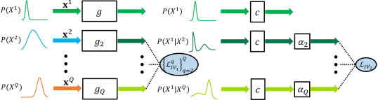
Figure 3. The proposed IV-DG framework. Feature extractor $g$ extracts input features of data and the networks $g_{2},...,g_{Q}$ learns conditional distributions $P(X^{1}|X^{2}),...,P(X^{1}|X^{Q})$, respectively. We learn invariant relationship between input features and label with a linear classifier $c$ via an IV-based two-stage method. It learns conditional distributions of $X^{1}$ given IV $X^{2},...,X^{Q}$ with loss $\{\mathcal{L}_{IV_{1}^{q}}\}_{q=2}^{Q}$ by optimizing $g_{2},...,g_{Q}$, then uses the estimated conditional distributions to optimize $c$ by predicting $Y^{1}$ with loss $\mathcal{L}_{IV_{2}}$. Hyper-parameters $\{\alpha_{q}\}_{q=2}^{Q}$ tune the influence of each IV, i.e., $X^{2},...,X^{Q}$, during training.

4.3. Framework and Algorithm

Algorithm 1 Instrumental Variable-driven Domain Generalization (IV-DG)

1:Datasets $\mathcal{D}_{1},...,\mathcal{D}_{Q}$, mixed dataset $\mathcal{D}_{mix}$, batchsize $B$, epochs $E^{pre}$, $E^{IV}$;

2:Well-trained $\hat{g}$ and $\hat{c}$;

3:for $epoch=1$ to $E^{pre}$ do     // model pretraining

4:     Sample $B$ examples from $\mathcal{D}_{mix}$ and optimize $g$, $c$ by minimizing $\mathcal{L}_{pre}$ as Eq. (14);

5:end for

6:Initialize $g_{q}$ by $g_{q}\leftarrow{g}$ for each $q\in\{2,...,Q\}$;

7:for $epoch=1$ to $E^{IV}$ do     // a two-stage IV method

8:     for $q=2$ to $Q$ do

9:         Sample $B$ examples from $\mathcal{D}_{1}$ and $\mathcal{D}_{q}$ and optimize $g_{q}$ by minimizing $\mathcal{L}_{IV_{1}^{q}}$ as Eq. (15);

10:     end for

11:     Sample $B$ examples from $\mathcal{D}_{q}$, $q=2,...,Q$, and optimize $c$ by minimizing $\mathcal{L}_{IV_{2}}$ as Eq. (16).

12:end for

Based on our analysis, we propose our method IV-DG with framework and algorithm as shown in Figure 3 and Algorithm 1, respectively. By following the common framework of DG, we adopt a feature extractor (backbone) $g$ which extracts the input features of high-dimensional data. We exploit a linear classifier $c$ to capture the invariant relationship between input features and label. We first pretrain $g$ and $c$ with mixed source data to initialize the ability of feature extraction and prediction, respectively, and then perform an IV-based two-stage method to debias $c$ for boosting the generalization ability of the model. Note that we can randomly select one source domain to be domain 1, while the other source domains to be domain 2,…,Q. We learn the invariant relationship between input features and label, i.e., an debiased classifier $c$, on domain 1, when the input features of the other domains are used as IVs.

We first pretrain the feature extractor $g$ and the classifier $c$ to initialize their ability of feature extraction and prediction, respectively. We randomly mix the sources $\{\mathcal{D}_{q}\}_{q=1}^{Q}$ to build a mixed dataset $\mathcal{D}_{mix}$ and use it to pretrain $g$ and $c$ with a cross-entropy classification loss $\mathcal{L}_{pre}$:

(14) $$\mathcal{L}_{pre}={\mathbb{E}_{(\mathrm{x},y)\in\mathcal{D}_{mix}}}\ell\left(c\circ{g}\left(\mathrm{x}\right),y\right),$$

where $\ell$ is the cross-entropy loss function. Through model pretraining, the feature extractor $g$ learns to extract feature representations of different datasets, and the classifier $c$ is initialized to classify the extracted feature representations. However, $c$ is biased because of the domain-specific information from the source datasets. We then perform an IV-based two-stage method to debias $c$ for learning the invariant relationship between the input feature (representations) and the labels.

Remark. Note that bias from source domains could be brought in this process, which may affect the learning of IV method in the following process. Despite this, this representation learning process could effectively help us extract features of each source domain for performing IV method. We assume that the introduced error will not have a significant impact on the final results.

In the stage 1 of the IV method, we assign the parameters of $g$ to $\{g_{q}\}_{q=2}^{Q}$ to initialize them, which is effective for the first stage of the IV method to our empirical experience. The two-stage IV method is conducted by: (i) learning conditional distributions of $X^{1}$ given IV $X^{2},...,X^{Q}$ via optimizing the networks $\{g_{q}\}_{q=2}^{Q}$; (ii) using the learned conditional distributions, i.e., $P(X^{1}|X^{2}),...,P(X^{1}|X^{Q})$, to optimize the classifier $c$ by predicting $Y^{1}$. Specifically, for the first stage, we use $g_{q}$ to estimate $P(X^{1}|X^{q})$ with the Maximum Mean Discrepancy (MMD) (Gretton et al., 2012), i.e., $d_{k}^{2}(v,w)\triangleq\|\mathbb{E}_{v}[\phi(g_{q}(\mathrm{x}^{q}))]-\mathbb{E}_{w}[\phi(g(\mathrm{x}^{1}))]\|_{\mathcal{H}_{k}}^{2}$. The distributions of the extracted input feature representations $g_{q}(\mathrm{x}^{q})$ and $g(x^{1})$, i.e., $v$ and $w$, satisfy $v=w$ iff $d_{k}^{2}(v,w)=0$. A characteristic kernel $k(g_{q}(\mathrm{x}^{q}),g(\mathrm{x}^{1}))=<\phi(g_{q}(\mathrm{x}^{q})),\phi(g(\mathrm{x}^{1}))>$ is defined as a convex combination of $o$ positive semi-definite kernels $\{k_{u}\}$, i.e., $\mathcal{K}\triangleq\left\{k=\sum_{u=1}^{o}\beta_{u}k_{u}:\sum_{u=1}^{o}\beta_{u}=1,\beta_{u}>=0,\forall{u}\right\}$, where $\beta_{u}$ guarantees the characteristic of multi-kernel $k$ (Long et al., 2015, 2017). We then estimate $P(X^{1}|X^{q})$ by optimizing $g_{q}$, which minimizes the MMD distance between the feature representations of $X^{1}$ and $X^{q}$ with the loss function

(15) $$\mathcal{L}_{IV_{1}}^{q}= p_{q,1}d_{k}^{2}\left(g_{q}\left(\mathrm{x}^{q}\right),g\left(\mathrm{x}^{1}\right)\right).$$

where $p_{q,1}:=\mathbb{I}(y^{q}=y^{1})$, i.e., $p_{q,1}=1$ when $y^{q}=y^{1}$, otherwise $p_{q,1}=0$. It is used to guarantee only the MMD distance of the input features from the same classes are minimized, which helps $g_{q}$ to learn a more accurate conditional distribution $P(X^{1}|X^{q})$ for each $q\in\{2,...,Q\}$.

In the stage 2 of the IV method, we sample points from the conditional distributions estimated in the first stage and use them to predict the labels. We optimize the classifier $c$ with a classification loss of the estimated conditional distribution, that is,

(16) $$\mathcal{L}_{IV_{2}}=\frac{1}{Q-1}\sum_{q=2}^{Q}\alpha_{q}\mathbb{E}_{(\mathrm{x}^{q},y^{q}),(\mathrm{x}^{1},y^{1})}\left[p_{q,1}\ell\left(c\circ g_{q}\left(\mathrm{x}^{q}\right),y^{1}\right)\right]$$

Since input features $X^{q}$ of each domain $q$, where $q\in\{2,...,Q\}$, could be used as an IV to capture the invariant relationship, we set hyper-parameters $\{\alpha_{q}\}_{q=2}^{Q}$ to tune the influence of each IV in the learning process for further improving model generalization. We use $p_{q,1}$ to guarantee the data used for debiasing are in the same classes. By optimizing $\mathcal{L}_{IV_{2}}$, the classifier $c$ removes the domain-specific bias of the source datasets introduced in the model pretraining. It allows $c$ to capture the domain-invariant relationship, improving the out-of-domain generalization ability.

Remark. Since we adopt $p_{q,1}$ to align the labels of domain 1 and domain $q$ ($q\in\{2,...,Q\}$), i.e., $Y^{1}$ and $Y^{q}$, at the two stages of IV-DG, IV process is implemented for each class during training. For example, when we sample data points from one class in domain $m$, we then sample data points from the same class in domain $n$ for learning (because we make $Y^{m}=Y^{n}$ in the training process). Even if there is not a triple of treatment $X^{m}$, instrument $X^{n}$, and outcome $Y^{m}$, we make $X^{m}$ and $X^{n}$ connected by letting $Y^{m}=Y^{n}$. Because $X^{m}$ and $X^{n}$ share the factor $F^{ivt}$ which is domain-invariant for a specific class when $Y^{m}=Y^{n}$. From another perspective, please see the Cats and Dogs dataset introduced in Section 5.3. Domain TB1 contains bright dogs and dark cats but domain TB2 contains dark dogs and bright cats. If we train a model on the domain TB1 or the domain TB2, the model would be biased by the brightness of the animals. In our IV-based method IV-DG, we can make $Y^{m}=Y^{n}=cat$ and let $X^{m}$ and $X^{n}$ be the cat features sampled from the domain TB1 and TB2, respectively, then capture the invariant relationship between the cat features and its label. Because the cat features from different domains share the factor $F^{ivt}$, which is the invariant characteristics of cats, like the shape of cats. The same process is performed for the dogs, too. Although we may not get triple samples from real-world datasets, we argue that our method still can capture stable relationship between input features and labels under the strong learning ability of deep neural networks, as shown by extensive experiments.

5. Experiments

We first conduct simulation experiments to verify the relationship learned by our method IV-DG. Then, we perform experiments on multiple real-world datasets to further testify the model generalization performance achieved by IV-DG.

5.1. Experiments on Simulated Datasets

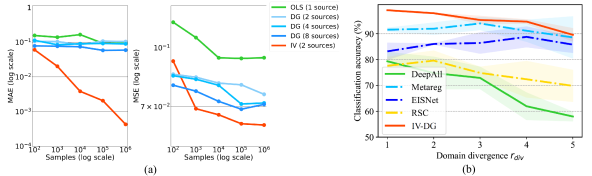
Figure 4. Simulation results in linear setting (a) for evaluating invariant relationship learning and target regression, and non-linear setting (b) for label prediction.

Linear simulations. We first evaluate the performance of invariant relationship estimation and target label prediction of IV method in linear domain generalization setting. We sample variables for each domain $m$ with $F^{ivt},F^{m}\sim\mathcal{N}(\mu_{f},1)$ and $e_{x}^{m},e_{y}^{m}\sim\mathcal{N}(\mu_{e},0.1)$. We sample $\mu_{f}$ once from uniform distribution $\mathrm{Unif}(-1,1)$ and sample $\mu_{e}$ once from $\mathrm{Unif}(-0.1,0.1)$ for each domain, making the divergence in each domain be random. We first consider linear setting with one-dimensional variables. The DGP of Figure 1 is assumed as

(17) $$X^{m}= \phi_{m}\cdot F^{ivt}+\alpha_{m}\cdot F^{m}+e_{x}^{m},$$

$$Y^{m}= \lambda_{ivt}\cdot X^{m}+\beta_{m}\cdot F^{m}+e_{y}^{m},$$

where $\lambda_{ivt}$ is the invariant relationship that we are interested in. We sample $\phi_{m}$, $\lambda_{ivt}$ once from $\mathrm{Unif}(-1,1)$ and sample $\alpha_{m}$, $\beta_{m}$ once from $\mathrm{Unif}(-0.5,0.5)$ for each domain. Note that we let domain-invariant factor and relationship, i.e., $F^{ivt}$ and $\lambda_{ivt}$, be the same in all domains. In each run, we randomly generate 8 source domains for training and a target domain for test with 20,000 points in each domain. We run each method with linear regression, and report the MAE of domain-invariant relationship estimation, i.e., $\mathbb{E}[\hat{\lambda}_{ivt}-\lambda_{ivt}]$, and the MSE of the target domain label $Y^{t}$ prediction, i.e., $\mathbb{E}[(\hat{Y^{t}}-Y^{t})]^{2}$. We implement OLS method by training the model on one source domain. The general DG method is implemented by estimating the coefficient in each domain and average them to get a robust coefficient. DG (n) sources is denoted as the coefficient estimated in this way with $n$ sources. IV method only needs two sources, i.e., the input features of one is used as IV to estimate the relationship on another source domain. We plot the results in Figure 4 (a). Obviously, with the increase of sample size, IV method outperforms others in invariant relationship $\lambda_{ivt}$ estimation and target label prediction when only using two source datasets. Although more source datasets allow the general DG methods to eliminate the domain-specific bias, they are still fooled by the introduced bias in data.

Non-linear simulations. We further evaluate the performance of our IV-based method IV-DG in non-linear domain generalization setting. Similar to the DGP in linear simulations, we sample variables $F^{ivt},F^{m}\sim\mathcal{N}(\mu_{f},1)$ and $e_{x}^{m},e_{y}^{m}\sim\mathcal{N}(\mu_{e},0.1)$. To evaluate the performance change with domain divergence, we sample $\mu_{f}$ from $\mathrm{Unif}(-r_{div},r_{div})$ for each domain, where a larger value of $r_{div}$ indicates the larger the domain divergence probably be. The DGP in non-linear setting is assumed as

(18) $$X^{m}= \phi_{m}\cdot F^{ivt}+\alpha_{m}\cdot F^{m}+e_{x}^{m},$$

$$Y^{m}= f_{ivt}(X^{m})+\beta_{m}\cdot F^{m}+e_{y}^{m}$$

The invariant relationship $\lambda_{ivt}$ is replaced with a non-linear function $f_{ivt}$, which is set to the absolute value function in the experiments. We set the dimensions of factor, i.e., $F^{ivt}$ and $F^{m}$, and input features, i.e., $X^{m}$, to 1500 and 600, respectively. We sample 10,000 data points each domain and divide them evenly into two classes with a threshold for the label $Y^{m}$. The goal is to accurately classify the target data by learning from 8 source datasets. We compare IV-DG with state-of-the-art DG methods (introduced in Section 2), i.e., Metareg (Balaji et al., 2018), EISNet (Wang et al., 2020), and RSC (Huang et al., 2020).

All the methods are implemented by their public code, but their networks are replaced with 4 fully-connected layers with 600, 256, 128, and 64 units, respectively, for fair comparison. We use SGD optimizer with learning rate 0.01, and run 4000 iterations with batchsize 64. The results in Figure 4 (b) illustrates that IV-DG with IV-based two-stage method outperforms other state-of-the-art DG methods. It is worth mentioning that IV-DG only utilizes two source domains to train, while other methods have 8 sources. We attribute the significant performance of IV-DG to its domain-invariant relationship learning ability, which makes full use of the two sources to obtain the invariant part contained in the conditional distribution of the labels given the input features. Besides, we find that data augmentation based method, i.e., Metareg and EISNet, show the robustness to the domain divergence. It is may because these methods generate various data distributions, and the models trained on the novel data could be more robustness.

5.2. Experiments on Real-World Datasets

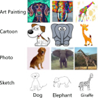
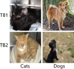
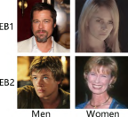
Figure 5. Example images of the adopted public datasets from left to right: PACS, Office-Home, Dogs and Cats, IMDB face. The former two datasets are used for the domain generalization task; and the latter two datasets are used for the unsupervised domain adaptation task.

Datasets and Implementations. We first conduct experiments on PACS (Li et al., 2017), which has 7 categories over 4 domains, that is, Art, Cartoon, Sketch, and Photo. Then we have Office-Home dataset (Venkateswara et al., 2017) that consists of 15,500 images of 65 categories over 4 domains, i.e., Art, Clipart, Product, and Real-World. Example images are shown in Figure 5. We follow the training and test split in previous works (Venkateswara et al., 2017; Li et al., 2017; Zhao et al., 2020), and perform leave-one-domain-out experiments, i.e., one domain is held out as the target domain for test. We follow (Carlucci et al., 2019; Dou et al., 2019; Huang et al., 2020) by using the pretrained ResNet-18 (He et al., 2016) network. We use SGD optimizer with learning rate 0.01 and batchsize 64. The epochs for the pretraining ($E^{pre}$) and the IV method ($E^{IV}$) are both set to 20. As one domain is chosen as the target domain, any of the rest domains can be used as $\mathcal{D}^{1}$, we use a held-out validation set, which is constructed from test domain by following the previous DG works (Zhao et al., 2020; Zhou et al., 2021, 2020c; Huang et al., 2020), to choose the optimal $\mathcal{D}^{1}$ as well as the corresponding hyper-parameters of Eq. (16). We conduct the experiments with CPU Intel i7-8700K $\times$ 1 and GPU Nvidia RTX 3090 $\times$ 1. We run each experiment 3 times with random seed, and cite the results of other methods in their papers (note that some baseline methods are not in Table 1 or Table 2 because their results are not reported in the corresponding paper).

Since when a domain is used as the target domain, any source could be treated as the $\mathcal{D}^{1}$, and other sources are used to learn the conditional distribution of $X^{1}$. Therefore, we first set all the weights (hyper-parameters) $\alpha$ to 1, and conduct different source combination experiments for PACS (Table 3) and Office-Home (Table 4) datasets. From Table 3 and Table 4, we observe that different choices for the first domain would not have a significant impact on the results, which shows the robustness of our method. After we have the best domain combinations, we then conduct weight combination experiments on PACS (Table 5) and Office-Home (Table 6) datasets. Finally, we use the “target-$\mathcal{D}^{1}$” combinations “Art-Photo”, “Cartoon-Photo”, “Photo-Art”, “Sketch-Photo” with weights $\alpha_{1}=1.25,\alpha_{2}=0.75$ for PACS dataset; and use “Art-Clipart”, “Clipart-Art”, “Product-Art”, “Real-World-Art” with weights $\alpha_{1}=1.5,\alpha_{2}=0.5$ for Office-Home datasets.

Table 1. Results (%) for domain generalization on PACS dataset.

Methods	Art	Cartoon	Photo	Sketch	Average
DeepAll (Carlucci et al., 2019)	78.96	72.93	96.28	70.59	79.94
JiGen (Carlucci et al., 2019)	79.42	75.25	96.03	71.35	80.51
MASF (Dou et al., 2019)	80.29	77.17	94.99	71.69	81.04
DGER (Zhao et al., 2020)	80.70	76.40	96.65	71.77	81.38
Epi-FCR (Li et al., 2019b)	82.1	77.0	93.9	73.0	81.5
MMLD (Matsuura and Harada, 2020)	81.28	77.16	96.09	72.29	81.83
EISNet (Wang et al., 2020)	81.89	76.44	95.93	74.33	82.15
L2A-OT (Zhou et al., 2020c)	83.3	78.2	96.2	73.6	82.8
DDAIG (Zhou et al., 2020b)	84.2	78.1	95.3	74.7	83.1
IRM (Arjovsky et al., 2019)	82.5	79.0	96.7	74.4	82.9
StableNet (Zhang et al., 2021)	80.16	74.15	94.24	70.10	79.66
IV-DG w/o IV	79.40 $\pm$ 0.10	76.93 $\pm$ 0.09	95.75 $\pm$ 0.10	74.44 $\pm$ 0.07	81.63 $\pm$ 0.03
IV-DG w/o pre	81.95 $\pm$ 0.25	77.55 $\pm$ 0.31	96.64 $\pm$ 0.34	75.65 $\pm$ 0.10	82.95 $\pm$ 0.14
IV-DG	83.36 $\pm$ 0.70	78.76 $\pm$ 0.08	96.87 $\pm$ 0.18	78.68 $\pm$ 0.96	84.42 $\pm$ 0.11

Table 2. Results (%) for domain generalization on Office-Home dataset.

Methods	Art	Clipart	Product	Real-World	Average
DeepAll (Carlucci et al., 2019)	52.15	45.86	70.86	73.15	60.51
JiGen (Carlucci et al., 2019)	53.04	47.51	71.47	72.79	61.20
DSON (Seo et al., 2020)	59.37	44.70	71.84	74.68	62.90
RSC (Huang et al., 2020)	58.42	47.90	71.63	74.54	63.12
IV-DG w/o IV	55.53 $\pm$ 0.21	45.92 $\pm$ 0.50	71.64 $\pm$ 0.35	74.49 $\pm$ 0.05	61.90 $\pm$ 0.20
IV-DG w/o pre	59.30 $\pm$ 0.06	47.65 $\pm$ 0.30	72.03 $\pm$ 0.57	75.55 $\pm$ 0.24	63.63 $\pm$ 0.11
IV-DG	60.40 $\pm$ 0.26	47.73 $\pm$ 0.28	72.63 $\pm$ 0.18	76.14 $\pm$ 0.10	64.23 $\pm$ 0.09

Table 3. Results (%) of different combinations for domain generalization on PACS dataset.

$\mathcal{D}^{1}$ $\backslash$ Target	Art	Cartoon	Photo	Sketch
Art	-	78.10 $\pm$0.37	97.17 $\pm$ 0.12	76.91 $\pm$ 0.03
Cartoon	82.21$\pm$0.97	-	96.75 $\pm$ 0.17	76.78 $\pm$ 0.98
Photo	83.77 $\pm$ 0.57	78.34 $\pm$ 0.58	-	77.48 $\pm$ 0.32
Sketch	81.46 $\pm$ 0.10	78.20 $\pm$0.76	97.01 $\pm$ 0.27	-

Table 4. Results (%) of different combinations for domain generalization on Office-Home dataset.

$\mathcal{D}^{1}$ $\backslash$ Target	Art	Clipart	Product	Real-World
Art	-	45.71 $\pm$ 0.20	72.31 $\pm$ 0.22	76.88 $\pm$ 0.08
Clipart	60.89 $\pm$ 0.17	-	72.21 $\pm$ 0.05	76.88 $\pm$ 0.12
Product	60.41 $\pm$ 0.20	45.10 $\pm$ 0.53	-	76.83 $\pm$ 0.14
Real-World	60.64 $\pm$ 0.29	45.65 $\pm$ 0.23	72.30 $\pm$ 0.41	-

Table 5. Results (%) with different weights for domain generalization on PACS dataset.

$\alpha_{1}$	$\alpha_{2}$	Art	Cartoon	Photo	Sketch	Average
0	2	82.68 $\pm$ 0.23	78.25 $\pm$ 0.15	97.15 $\pm$ 0.18	77.43 $\pm$ 0.29	83.88 $\pm$ 0.88
0.25	1.75	82.33 $\pm$ 0.30	79.15 $\pm$ 0.57	97.07 $\pm$ 0.12	78.16 $\pm$ 0.64	84.18 $\pm$ 0.26
0.5	1.5	82.21 $\pm$ 0.75	78.19 $\pm$ 0.50	97.11 $\pm$ 0.07	77.51 $\pm$ 0.96	83.75 $\pm$ 0.09
0.75	1.25	82.60 $\pm$ 0.88	78.88 $\pm$ 0.89	97.09 $\pm$ 0.03	78.65 $\pm$ 0.71	84.31 $\pm$ 0.62
1	1	83.77 $\pm$ 0.57	78.34 $\pm$ 0.58	97.17 $\pm$ 0.12	77.48 $\pm$ 0.32	84.19 $\pm$ 0.25
1.25	0.75	83.36 $\pm$ 0.70	78.76 $\pm$ 0.08	96.87 $\pm$ 0.18	78.68 $\pm$ 0.96	84.42 $\pm$ 0.11
1.5	0.5	81.89 $\pm$ 0.08	78.60 $\pm$ 0.29	97.35 $\pm$ 0.12	78.20 $\pm$ 1.02	84.01 $\pm$ 0.18
1.75	0.25	81.98 $\pm$ 0.15	79.17 $\pm$ 0.73	96.87 $\pm$ 0.38	78.53 $\pm$ 0.14	84.14 $\pm$ 0.10
2	0	82.14 $\pm$ 0.17	78.22 $\pm$ 0.10	97.05 $\pm$ 0.12	77.46 $\pm$ 1.58	83.72 $\pm$ 0.38

Table 6. Results (%) with different weights for domain generalization on Office-Home dataset.

$\alpha_{1}$	$\alpha_{2}$	Art	Clipart	Product	Real-World	Average
0	2	60.63 $\pm$ 0.25	47.40 $\pm$ 0.08	72.51 $\pm$ 0.08	76.12 $\pm$ 0.59	64.16 $\pm$ 0.10
0.25	1.75	60.71 $\pm$ 0.13	46.48 $\pm$ 0.26	72.59 $\pm$ 0.08	76.93 $\pm$ 0.17	64.18 $\pm$ 0.02
0.5	1.5	60.79 $\pm$ 0.11	46.18 $\pm$ 0.16	72.62 $\pm$ 0.13	76.10 $\pm$ 0.17	63.92 $\pm$ 0.04
0.75	1.25	60.53 $\pm$ 0.09	46.36 $\pm$ 0.36	72.60 $\pm$ 0.14	76.69 $\pm$ 0.11	64.05 $\pm$ 0.08
1	1	60.89 $\pm$ 0.17	45.71 $\pm$ 0.20	72.31 $\pm$ 0.22	76.88 $\pm$ 0.08	63.95 $\pm$ 0.05
1.25	0.75	60.90 $\pm$ 0.39	46.20 $\pm$ 0.35	72.54 $\pm$ 0.23	77.06 $\pm$ 0.25	64.17 $\pm$ 0.10
1.5	0.5	60.40 $\pm$ 0.26	47.73 $\pm$ 0.28	72.63 $\pm$ 0.18	76.14 $\pm$ 0.10	64.23 $\pm$ 0.09
1.75	0.25	60.58 $\pm$ 0.20	46.48 $\pm$ 0.21	72.54 $\pm$ 0.14	76.89 $\pm$ 0.34	64.12 $\pm$ 0.11
2	0	60.95 $\pm$ 0.15	46.28 $\pm$ 0.11	72.44 $\pm$ 0.04	76.88 $\pm$ 0.21	64.14 $\pm$ 0.04

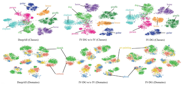
Figure 6. T-SNE visulazation of the learned feature representations of DeepAll, IV-DG w/o IV, and IV-DG, on PACS dataset. Different colors in the above and below sub-figures represent different classes and domains, respectively. The points gather separately for classes and compactly for domains indicates the learned feature representations are more discriminative and domain-agnostic, respectively.

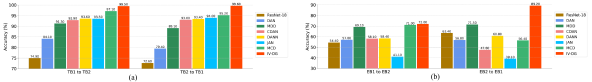
Figure 7. Results for unsupervised domain adaptation task on Dogs and Cats (a) and IMDB face (b) datasets.

Results. Table 1 and Table 2 report the results on PACS and Office-Home datasets, respectively. Note that the DeepAll method is implemented by training the model with general supervised learning on the aggregation of all the source datasets. We first find that IV-DG outperforms other methods on both datasets by performing the best on most of the DG sub-tasks and achieving the highest averaged accuracy. We attribute it to that IV-DG learns to capture the invariant part (relationship) contained in the conditional distribution for better model generalization. We let IV-DG discard the IV method and pretraining as w/o IV and w/o pre, respectively in Table 1 and Table 2. It shows that each part is important for IV-DG to yield significant performance, especially the IV method. It is may because the pretrainig initialize the discriminability of the feature extractor for better conditional distribution estimation, and the IV method helps model learn domain-invariant relationship by debiasing the classifier. We plot the t-SNE feature visualization in Figure 6. It indicates that IV method helps IV-DG to learn discriminative and domain-invaraint feature during the IV-based two-stage process by separating the features of different classes while aggregating the features of different domains.

5.3. Experiments on Biased Data

We also evaluate IV-DG on the unsupervised domain adaptation (UDA) task where IV-DG uses the input features of the target dataset as IVs to learn the invariant relationship with the given source dataset. We adopt two biased datasets for this task. The first is Dogs and Cats (Kim et al., 2019), where TB1 domain contains bright dogs and dark cats; but TB2 domain contains dark dogs and bright cats. The second is IMDB face dataset (Kim et al., 2019). Women in a domain EB1 aged 0-29 and in another domain EB2 aged 40+; but men in EB1 aged 40+ and in EB2 aged 0-29. There is clear bias between the domains in the two datasets, which challenges the methods to learn stable relationship between the images and labels. We compare IV-DG with representative DA approaches, DAN (Long et al., 2015), DANN (Ganin and Lempitsky, 2015), JAN (Long et al., 2017), MDD (Zhang et al., 2019b), CDAN (Long et al., 2018), MCD (Saito et al., 2018). All the experiments are implemented using the same training setting for fair comparison. Following (Long et al., 2018; Xu et al., 2019; Liang et al., 2020), We employ the pre-trained ResNet-50 (He et al., 2016) as the feature extractor, where the last layer is replaced by one FC layer with 256 units. Classifier is a FC layer put after feature extractor for classification. We train each method through back-propagation by SGD with batch-size 64, learning rate 0.01, momentum 0.9, and weight decay 0.001. Each method are run 10 epochs on Dogs and Cats dataset and 5 epochs on IMDB face dataset for fair comparison. Results in Figure 7 show that IV-DG performs much better than others on the two challenging biased datasets. Moreover, we find that IV-DG achieves significant improvement on IMDB face dataset. It is probably because IV method needs sufficient samples to obtain invariant relationship (see Figure 4), and IMDB face is a large dataset with 460,723 images.

6. Conclusions

In this paper, we first give a causal view on the domain generalization problem, and then propose to learn domain-invariant relationship with instrumental variable via an IV-based two-stage method. Extensive experiments show the significant performance of our method. Our paper benefits the research of domain generalization and may not have negative impact of society to our knowledge.

Despite the great performance achieved by our method, there are some limitations. First, our method is based on the assumed causal graph. Some assumptions, e.g., $F^{m}$ is the domain-specific factor changed with the background but uncorrelated to the invariant factor of the recognized animals, may not hold in real-world scenarios. For example, lambs with their size and limbs probably in grassland. Second, since our theoretical analyses relies on the assumption of linearity and additivity, hence it may be not leading to stable prediction on out-of-distribution target data when the data generating process of domain-invariant factor $F^{ivt}$, domain-specific factor $F^{m}$, and error term $e_{x}^{m}$, $e_{y}^{m}$ is a highly non-linear complex function (Rothenhäusler et al., 2021; Lin et al., 2022b). For example, the bias of domain-specific factor (confounder) $F^{m}$, which causes the distribution shift, may not be completely removed if $F^{m}$ is connected with $f(X^{m})$ via an unknown non-linear function. In the future work, we aim to use more moderate assumptions to build the model, which could achieve better performance.

- (1)
- Angrist and Pischke (2008) Joshua D Angrist and Jörn-Steffen Pischke. 2008. Mostly harmless econometrics: An empiricist’s companion. Princeton university press.
- Arjovsky et al. (2019) Martin Arjovsky, Léon Bottou, Ishaan Gulrajani, and David Lopez-Paz. 2019. Invariant risk minimization. arXiv preprint arXiv:1907.02893 (2019).
- Balaji et al. (2018) Yogesh Balaji, Swami Sankaranarayanan, and Rama Chellappa. 2018. Metareg: Towards domain generalization using meta-regularization. In Advances in Neural Information Processing Systems (NeurIPS). 998–1008.
- Ben-David et al. (2010) Shai Ben-David, John Blitzer, Koby Crammer, Alex Kulesza, Fernando Pereira, and Jennifer Wortman Vaughan. 2010. A theory of learning from different domains. Machine learning 79, 1-2 (2010), 151–175.
- Bennett et al. (2019) Andrew Bennett, Nathan Kallus, and Tobias Schnabel. 2019. Deep generalized method of moments for instrumental variable analysis. In Advances in Neural Information Processing Systems (NeurIPS). 3564–3574.
- Blanchard et al. (2011) Gilles Blanchard, Gyemin Lee, and Clayton Scott. 2011. Generalizing from several related classification tasks to a new unlabeled sample. Advances in neural information processing systems (NeurIPS) 24 (2011), 2178–2186.
- Cai et al. (2019) Guanyu Cai, Yuqin Wang, Lianghua He, and MengChu Zhou. 2019. Unsupervised domain adaptation with adversarial residual transform networks. IEEE transactions on neural networks and learning systems (TNNLS) 31, 8 (2019), 3073–3086.
- Carlucci et al. (2019) Fabio Maria Carlucci, Antonio D’Innocente, S. Bucci, B. Caputo, and T. Tommasi. 2019. Domain Generalization by Solving Jigsaw Puzzles. Proceedings of the IEEE Conference on Computer Vision and Pattern Recognition (CVPR) (2019), 2224–2233.
- Chattopadhyay et al. (2020) Prithvijit Chattopadhyay, Yogesh Balaji, and Judy Hoffman. 2020. Learning to balance specificity and invariance for in and out of domain generalization. In European Conference on Computer Vision (ECCV). Springer, 301–318.
- Chattopadhyay et al. (2012) Rita Chattopadhyay, Qian Sun, Wei Fan, Ian Davidson, Sethuraman Panchanathan, and Jieping Ye. 2012. Multisource domain adaptation and its application to early detection of fatigue. ACM Transactions on Knowledge Discovery from Data (TKDD) 6, 4 (2012), 1–26.
- Christiansen et al. (2021) Rune Christiansen, Niklas Pfister, Martin Emil Jakobsen, Nicola Gnecco, and Jonas Peters. 2021. A causal framework for distribution generalization. IEEE Transactions on Pattern Analysis and Machine Intelligence (2021).
- Dou et al. (2019) Qi Dou, Daniel Coelho de Castro, Konstantinos Kamnitsas, and Ben Glocker. 2019. Domain generalization via model-agnostic learning of semantic features. In Advances in Neural Information Processing Systems (NeurIPS). 6450–6461.
- Fan et al. (2020) Jingtao Fan, Lu Fang, Jiamin Wu, Yuchen Guo, and Qionghai Dai. 2020. From brain science to artificial intelligence. Engineering 6, 3 (2020), 248–252.
- Ganin and Lempitsky (2015) Yaroslav Ganin and Victor Lempitsky. 2015. Unsupervised domain adaptation by backpropagation. In International conference on machine learning (ICML). PMLR, 1180–1189.
- Ghifary et al. (2015) Muhammad Ghifary, W Bastiaan Kleijn, Mengjie Zhang, and David Balduzzi. 2015. Domain generalization for object recognition with multi-task autoencoders. In Proceedings of the IEEE international conference on computer vision (ICCV). 2551–2559.
- Gong et al. (2016) Mingming Gong, Kun Zhang, Tongliang Liu, Dacheng Tao, Clark Glymour, and Bernhard Schölkopf. 2016. Domain adaptation with conditional transferable components. In International conference on machine learning. PMLR, 2839–2848.
- Gretton et al. (2012) Arthur Gretton, Karsten M Borgwardt, Malte J Rasch, Bernhard Schölkopf, and Alexander Smola. 2012. A kernel two-sample test. The Journal of Machine Learning Research (JMLR) 13, 1 (2012), 723–773.
- Hartford et al. (2017) Jason Hartford, Greg Lewis, Kevin Leyton-Brown, and Matt Taddy. 2017. Deep IV: A flexible approach for counterfactual prediction. In International Conference on Machine Learning (ICML). 1414–1423.
- He et al. (2016) Kaiming He, Xiangyu Zhang, Shaoqing Ren, and Jian Sun. 2016. Deep residual learning for image recognition. In Proceedings of the IEEE Conference on Computer Vision and Pattern Recognition (CVPR). 770–778.
- Heyde (2006) CC Heyde. 2006. Central limit theorem. Encyclopedia of actuarial science 1 (2006).
- Huang et al. (2020) Zeyi Huang, Haohan Wang, Eric P. Xing, and Dong Huang. 2020. Self-challenging Improves Cross-Domain Generalization. In European Conference on Computer Vision (ECCV). 124–140.
- Kim et al. (2019) Byungju Kim, Hyunwoo Kim, Kyungsu Kim, Sungjin Kim, and Junmo Kim. 2019. Learning not to learn: Training deep neural networks with biased data. In Conference on Computer Vision and Pattern Recognition (CVPR). 9012–9020.
- Kuang et al. (2020) Kun Kuang, Lian Li, Zhi Geng, Lei Xu, Kun Zhang, Beishui Liao, Huaxin Huang, Peng Ding, Wang Miao, and Zhichao Jiang. 2020. Causal inference. Engineering 6, 3 (2020), 253–263.
- Li et al. (2018d) Da Li, Yongxin Yang, Yi-Zhe Song, and Timothy Hospedales. 2018d. Learning to generalize: Meta-learning for domain generalization. In Proceedings of the AAAI Conference on Artificial Intelligence (AAAI), Vol. 32.
- Li et al. (2017) Da Li, Yongxin Yang, Yi-Zhe Song, and Timothy M Hospedales. 2017. Deeper, broader and artier domain generalization. In Proceedings of the IEEE International Conference on Computer Vision (ICCV). 5542–5550.
- Li et al. (2019b) Da Li, J. Zhang, Yongxin Yang, Cong Liu, Yi-Zhe Song, and Timothy M. Hospedales. 2019b. Episodic Training for Domain Generalization. Proceedings of the IEEE International Conference on Computer Vision (ICCV) (2019), 1446–1455.
- Li et al. (2018b) Haoliang Li, Sinno Jialin Pan, Shiqi Wang, and Alex C Kot. 2018b. Domain generalization with adversarial feature learning. In Proceedings of the IEEE Conference on Computer Vision and Pattern Recognition (CVPR). 5400–5409.
- Li et al. (2020) Haoliang Li, Yufei Wang, Renjie Wan, Shiqi Wang, Tie-Qiang Li, and Alex C. Kot. 2020. Domain Generalization for Medical Imaging Classification with Linear-Dependency Regularization. In Advances in Neural Information Processing Systems (NeurIPS).
- Li et al. (2018a) Ya Li, Mingming Gong, Xinmei Tian, Tongliang Liu, and Dacheng Tao. 2018a. Domain generalization via conditional invariant representations. In Proceedings of the AAAI Conference on Artificial Intelligence, Vol. 32.
- Li et al. (2018c) Ya Li, Xinmei Tian, Mingming Gong, Yajing Liu, Tongliang Liu, Kun Zhang, and Dacheng Tao. 2018c. Deep domain generalization via conditional invariant adversarial networks. In Proceedings of the European Conference on Computer Vision (ECCV). 624–639.
- Li et al. (2019a) Yiying Li, Yongxin Yang, Wei Zhou, and Timothy Hospedales. 2019a. Feature-critic networks for heterogeneous domain generalization. In International Conference on Machine Learning (ICML). PMLR, 3915–3924.
- Liang et al. (2020) Jian Liang, D. Hu, and Jiashi Feng. 2020. Do We Really Need to Access the Source Data? Source Hypothesis Transfer for Unsupervised Domain Adaptation. In International Conference on Machine Learning (ICML). PMLR.
- Lin et al. (2022b) Wanyu Lin, Hao Lan, Hao Wang, and Baochun Li. 2022b. Orphicx: A causality-inspired latent variable model for interpreting graph neural networks. In Proceedings of the IEEE/CVF Conference on Computer Vision and Pattern Recognition. 13729–13738.
- Lin et al. (2022a) Yong Lin, Hanze Dong, Hao Wang, and Tong Zhang. 2022a. Bayesian Invariant Risk Minimization. In Proceedings of the IEEE/CVF Conference on Computer Vision and Pattern Recognition. 16021–16030.
- Long et al. (2015) Mingsheng Long, Yue Cao, Jianmin Wang, and Michael Jordan. 2015. Learning transferable features with deep adaptation networks. In International conference on machine learning (ICML). PMLR, 97–105.
- Long et al. (2018) Mingsheng Long, Zhangjie Cao, Jianmin Wang, and Michael I Jordan. 2018. Conditional adversarial domain adaptation. In Advances in neural information processing systems (NeurIPS). 1640–1650.
- Long et al. (2017) Mingsheng Long, Han Zhu, Jianmin Wang, and Michael I Jordan. 2017. Deep transfer learning with joint adaptation networks. In International conference on machine learning (ICML). PMLR, 2208–2217.
- Lu et al. (2022) Wang Lu, Jindong Wang, Haoliang Li, Yiqiang Chen, and Xing Xie. 2022. Domain-invariant Feature Exploration for Domain Generalization. arXiv preprint arXiv:2207.12020 (2022).
- Lv et al. (2023a) Zheqi Lv, Zhengyu Chen, Shengyu Zhang, Kun Kuang, Wenqiao Zhang, Mengze Li, Beng Chin Ooi, and Fei Wu. 2023a. IDEAL: Toward High-efficiency Device-Cloud Collaborative and Dynamic Recommendation System. arXiv preprint arXiv:2302.07335 (2023).
- Lv et al. (2022) Zheqi Lv, Feng Wang, Shengyu Zhang, Kun Kuang, Hongxia Yang, and Fei Wu. 2022. Personalizing Intervened Network for Long-tailed Sequential User Behavior Modeling. arXiv preprint arXiv:2208.09130 (2022).
- Lv et al. (2023b) Zheqi Lv, Wenqiao Zhang, Shengyu Zhang, Kun Kuang, Feng Wang, Yongwei Wang, Zhengyu Chen, Tao Shen, Hongxia Yang, Beng Chin Ooi, and Fei Wu. 2023b. DUET: A Tuning-Free Device-Cloud Collaborative Parameters Generation Framework for Efficient Device Model Generalization. In Proceedings of the ACM Web Conference 2023.
- Ma et al. (2021) Ao Ma, Jingjing Li, Ke Lu, Lei Zhu, and Heng Tao Shen. 2021. Adversarial Entropy Optimization for Unsupervised Domain Adaptation. IEEE Transactions on Neural Networks and Learning Systems (TNNLS) (2021).
- Ma et al. (2022) Xu Ma, Junkun Yuan, Yen-wei Chen, Ruofeng Tong, and Lanfen Lin. 2022. Attention-based cross-layer domain alignment for unsupervised domain adaptation. Neurocomputing 499 (2022), 1–10.
- Mahajan et al. (2021) Divyat Mahajan, Shruti Tople, and Amit Sharma. 2021. Domain generalization using causal matching. In International Conference on Machine Learning. PMLR, 7313–7324.
- Mao et al. (2021) Chengzhi Mao, Augustine Cha, Amogh Gupta, Hao Wang, Junfeng Yang, and Carl Vondrick. 2021. Generative interventions for causal learning. In Proceedings of the IEEE/CVF Conference on Computer Vision and Pattern Recognition. 3947–3956.
- Mao et al. (2022) Chengzhi Mao, Kevin Xia, James Wang, Hao Wang, Junfeng Yang, Elias Bareinboim, and Carl Vondrick. 2022. Causal Transportability for Visual Recognition. In Proceedings of the IEEE/CVF Conference on Computer Vision and Pattern Recognition. 7521–7531.
- Matsuura and Harada (2020) T. Matsuura and T. Harada. 2020. Domain Generalization Using a Mixture of Multiple Latent Domains. In Proceedings of the AAAI Conference on Artificial Intelligence (AAAI).
- Miao et al. (2022) Qiaowei Miao, Junkun Yuan, and Kun Kuang. 2022. Domain Generalization via Contrastive Causal Learning. arXiv preprint arXiv:2210.02655 (2022).
- Newey and Powell (2003) Whitney K Newey and James L Powell. 2003. Instrumental variable estimation of nonparametric models. Econometrica (2003), 1565–1578.
- Niu et al. (2023) Ziwei Niu, Junkun Yuan, Xu Ma, Yingying Xu, Jing Liu, Yen-Wei Chen, Ruofeng Tong, and Lanfen Lin. 2023. Knowledge Distillation-based Domain-invariant Representation Learning for Domain Generalization. IEEE Transactions on Multimedia (2023).
- Pearl (2009) Judea Pearl. 2009. Causality. Cambridge university press.
- Peng et al. (2019) Xingchao Peng, Qinxun Bai, Xide Xia, Zijun Huang, Kate Saenko, and Bo Wang. 2019. Moment matching for multi-source domain adaptation. In Proceedings of the IEEE International Conference on Computer Vision (ICCV). 1406–1415.
- Piratla et al. (2020) Vihari Piratla, Praneeth Netrapalli, and Sunita Sarawagi. 2020. Efficient Domain Generalization via Common-Specific Low-Rank Decomposition. In International Conference on Machine Learning (ICML).
- Qiao et al. (2020) Fengchun Qiao, Long Zhao, and Xi Peng. 2020. Learning to learn single domain generalization. In Proceedings of the IEEE Conference on Computer Vision and Pattern Recognition. 12556–12565.
- Quionero-Candela et al. (2009) Joaquin Quionero-Candela, Masashi Sugiyama, Anton Schwaighofer, and Neil D Lawrence. 2009. Dataset shift in machine learning. The MIT Press.
- Ren et al. (2020) Kui Ren, Tianhang Zheng, Zhan Qin, and Xue Liu. 2020. Adversarial attacks and defenses in deep learning. Engineering 6, 3 (2020), 346–360.
- Rothenhäusler et al. (2021) Dominik Rothenhäusler, Nicolai Meinshausen, Peter Bühlmann, and Jonas Peters. 2021. Anchor regression: Heterogeneous data meet causality. Journal of the Royal Statistical Society: Series B (Statistical Methodology) 83, 2 (2021), 215–246.
- Saito et al. (2018) Kuniaki Saito, Kohei Watanabe, Yoshitaka Ushiku, and Tatsuya Harada. 2018. Maximum classifier discrepancy for unsupervised domain adaptation. In Proceedings of the IEEE Conference on Computer Vision and Pattern Recognition (CVPR). 3723–3732.
- Seo et al. (2020) Seonguk Seo, Yumin Suh, D. Kim, Jongwoo Han, and B. Han. 2020. Learning to Optimize Domain Specific Normalization for Domain Generalization. In European Conference on Computer Vision (ECCV).
- Shankar et al. (2018) S. Shankar, Vihari Piratla, Soumen Chakrabarti, S. Chaudhuri, P. Jyothi, and Sunita Sarawagi. 2018. Generalizing Across Domains via Cross-Gradient Training. In International Conference on Learning Representations (ICLR).
- Singh et al. (2019) Rahul Singh, Maneesh Sahani, and Arthur Gretton. 2019. Kernel instrumental variable regression. In Advances in Neural Information Processing Systems (NeurIPS). 4593–4605.
- Venkateswara et al. (2017) Hemanth Venkateswara, Jose Eusebio, Shayok Chakraborty, and Sethuraman Panchanathan. 2017. Deep hashing network for unsupervised domain adaptation. In Proceedings of the IEEE Conference on Computer Vision and Pattern Recognition (CVPR). 5018–5027.
- Volpi et al. (2018) Riccardo Volpi, Hongseok Namkoong, Ozan Sener, John C Duchi, Vittorio Murino, and Silvio Savarese. 2018. Generalizing to unseen domains via adversarial data augmentation. In Advances in neural information processing systems (NeurIPS). 5334–5344.
- Wang et al. (2020) Shujun Wang, Lequan Yu, Caizi Li, Chi-Wing Fu, and P. Heng. 2020. Learning from Extrinsic and Intrinsic Supervisions for Domain Generalization. In European conference on computer vision (ECCV).
- Wang et al. (2021) Yufei Wang, Haoliang Li, Lap-Pui Chau, and Alex C Kot. 2021. Variational disentanglement for domain generalization. arXiv preprint arXiv:2109.05826 (2021).
- Wright (1928) Philip G Wright. 1928. Tariff on animal and vegetable oils. Macmillan Company, New York.
- Wu et al. (2022) Anpeng Wu, Junkun Yuan, Kun Kuang, Bo Li, Runze Wu, Qiang Zhu, Yue Ting Zhuang, and Fei Wu. 2022. Learning decomposed representations for treatment effect estimation. IEEE Transactions on Knowledge and Data Engineering (2022).
- Wu and Ng (2022) Hanrui Wu and Michael K Ng. 2022. Multiple graphs and low-rank embedding for multi-source heterogeneous domain adaptation. ACM Transactions on Knowledge Discovery from Data (TKDD) 16, 4 (2022), 1–25.
- Xu et al. (2019) Ruijia Xu, Guanbin Li, Jihan Yang, and Liang Lin. 2019. Larger norm more transferable: An adaptive feature norm approach for unsupervised domain adaptation. In Proceedings of the IEEE International Conference on Computer Vision (ICCV). 1426–1435.
- Yang et al. (2021) Shuai Yang, Kui Yu, Fuyuan Cao, Lin Liu, Hao Wang, and Jiuyong Li. 2021. Learning causal representations for robust domain adaptation. IEEE Transactions on Knowledge and Data Engineering (2021).
- Yuan et al. (2022a) Junkun Yuan, Xu Ma, Defang Chen, Kun Kuang, Fei Wu, and Lanfen Lin. 2022a. Label-Efficient Domain Generalization via Collaborative Exploration and Generalization. In Proceedings of the 30th ACM International Conference on Multimedia. 2361–2370.
- Yuan et al. (2023a) Junkun Yuan, Xu Ma, Defang Chen, Kun Kuang, Fei Wu, and Lanfen Lin. 2023a. Domain-specific bias filtering for single labeled domain generalization. International Journal of Computer Vision 131, 2 (2023), 552–571.
- Yuan et al. (2023b) Junkun Yuan, Xu Ma, Defang Chen, Fei Wu, Lanfen Lin, and Kun Kuang. 2023b. Collaborative Semantic Aggregation and Calibration for Federated Domain Generalization. IEEE Transactions on Knowledge and Data Engineering (2023).
- Yuan et al. (2022b) Junkun Yuan, Anpeng Wu, Kun Kuang, Bo Li, Runze Wu, Fei Wu, and Lanfen Lin. 2022b. Auto iv: Counterfactual prediction via automatic instrumental variable decomposition. ACM Transactions on Knowledge Discovery from Data (TKDD) 16, 4 (2022), 1–20.
- Zhang et al. (2020b) Cheng Zhang, Kun Zhang, and Yingzhen Li. 2020b. A Causal View on Robustness of Neural Networks. In Advances in Neural Information Processing Systems (NeurIPS).
- Zhang et al. (2015) Kun Zhang, Mingming Gong, Bernhard Schölkopf, et al. 2015. Multi-Source Domain Adaptation: A Causal View.. In AAAI Conference on Artificial Intelligence (AAAI), Vol. 1. 3150–3157.
- Zhang et al. (2020a) Kun Zhang, Mingming Gong, Petar Stojanov, Biwei Huang, Qingsong Liu, and Clark Glymour. 2020a. Domain adaptation as a problem of inference on graphical models. Advances in Neural Information Processing Systems (NeurIPS) 33 (2020).
- Zhang et al. (2013) Kun Zhang, Bernhard Schölkopf, Krikamol Muandet, and Zhikun Wang. 2013. Domain adaptation under target and conditional shift. In International Conference on Machine Learning (ICML). 819–827.
- Zhang et al. (2019a) Lei Zhang, Jingru Fu, Shanshan Wang, David Zhang, Zhaoyang Dong, and CL Philip Chen. 2019a. Guide subspace learning for unsupervised domain adaptation. IEEE transactions on neural networks and learning systems (TNNLS) 31, 9 (2019), 3374–3388.
- Zhang et al. (2021) Xingxuan Zhang, Peng Cui, Renzhe Xu, Linjun Zhou, Yue He, and Zheyan Shen. 2021. Deep stable learning for out-of-distribution generalization. In Proceedings of the IEEE/CVF Conference on Computer Vision and Pattern Recognition. 5372–5382.
- Zhang et al. (2019b) Yuchen Zhang, Tianle Liu, Mingsheng Long, and Michael I. Jordan. 2019b. Bridging Theory and Algorithm for Domain Adaptation. In International Conference on Machine Learning (ICML).
- Zhao et al. (2020) Shanshan Zhao, M. Gong, T. Liu, H. Fu, and Dacheng Tao. 2020. Domain Generalization via Entropy Regularization. In Advances in Neural Information Processing Systems (NeurIPS).
- Zhou et al. (2020b) Kaiyang Zhou, Yongxin Yang, Timothy Hospedales, and Tao Xiang. 2020b. Deep domain-adversarial image generation for domain generalisation. In Proceedings of the AAAI Conference on Artificial Intelligence (AAAI), Vol. 34. 13025–13032.
- Zhou et al. (2020c) Kaiyang Zhou, Yongxin Yang, Timothy Hospedales, and Tao Xiang. 2020c. Learning to generate novel domains for domain generalization. In European Conference on Computer Vision (ECCV). 561–578.
- Zhou et al. (2021) Kaiyang Zhou, Yongxin Yang, Yu Qiao, and Tao Xiang. 2021. Domain Generalization with Mixstyle. In International Conference on Learning Representations (ICLR).
- Zhou et al. (2020a) Ming Zhou, Nan Duan, Shujie Liu, and Heung-Yeung Shum. 2020a. Progress in neural NLP: modeling, learning, and reasoning. Engineering 6, 3 (2020), 275–290.