An Efficient Procedure for Mining Egocentric Temporal Motifs

Abstract

Temporal graphs are structures which model relational data between entities that change over time. Due to the complex structure of data, mining statistically significant temporal subgraphs, also known as temporal motifs, is a challenging task. In this work, we present an efficient technique for extracting temporal motifs in temporal networks. Our method is based on the novel notion of egocentric temporal neighborhoods, namely multi-layer structures centered on an ego node. Each temporal layer of the structure consists of the first-order neighborhood of the ego node, and corresponding nodes in sequential layers are connected by an edge. The strength of this approach lies in the possibility of encoding these structures into a unique bit vector, thus bypassing the problem of graph isomorphism in searching for temporal motifs. This allows our algorithm to mine substantially larger motifs with respect to alternative approaches. Furthermore, by bringing the focus on the temporal dynamics of the interactions of a specific node, our model allows to mine temporal motifs which are visibly interpretable. Experiments on a number of complex networks of social interactions confirm the advantage of the proposed approach over alternative non-egocentric solutions. The egocentric procedure is indeed more efficient in revealing similarities and discrepancies among different social environments, independently of the different technologies used to collect data, which instead affect standard non-egocentric measures.
keywords:Network motifs, Temporal networks, Graph mining, Social interaction networks, Sociopatterns

1 Introduction

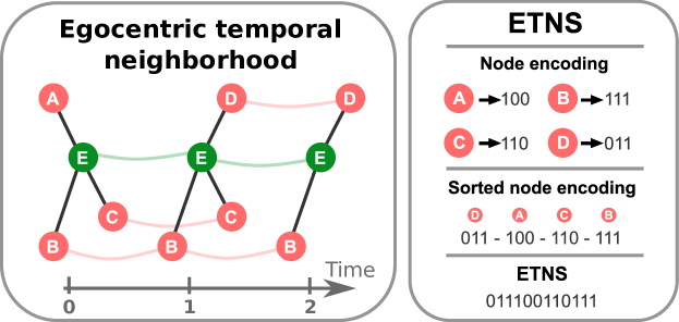
Figure 1: Graphical summary of the procedure for extracting egocentric temporal motifs. The left panel shows the egocentric temporal neighborhood of the ego node $E$ (in green), with temporal order two and initial time instant zero. Black edges connect the central node with its neighbors (in red) at each time step, while green (resp. red) edges connect consecutive occurrences of the central (resp. a neighboring) node along the time sequence. The right panel shows how the corresponding egocentric temporal neighborhood signature (ETNS) is computed. Each neighboring node is encoded into a bit vector indicating the time slots when it is present. The node encodings are lexicographically sorted first and then concatenated to generate the signature.

Complex networks play a pivotal role in describing and analyzing complex systems in multiple natural and artificial scenarios, representing a fundamental tool for modeling biological, cognitive and social systems Newman (2010). Interestingly, the small substructures that compose the complex topology of a network are sometimes recurrently emerging as essential constituents for the specific network at hand. They consist in sub-networks composed by a small number of nodes with a specific structure of connections. The substructures which are identified as the most significant take the name of motifs Milo et al. (2002); Alon (2007). The significance of each specific substructure within the overall network architecture is assessed in relation to its frequency and usually referring to a null model: a structure is considered a motif if the number of its occurrences in the network is substantially higher than the number of occurrences in the null model.
The identification of specific repeated motifs offers a unique opportunity to investigate the complex and intricate dynamics of human behavior and interactions Wasserman et al. (1994); Milgram (1967). As a matter of fact, when analyzing social dynamics we usually need to deal with time-dependent structures Kossinets and Watts (2006); Kossinets et al. (2008). Social interactions are indeed characterized by links which appear and disappear in time and are associated with variable duration. The appropriate topological tool to describe systems of dynamical interactions is represented by temporal networks with a fixed set of nodes connected by edges that vary over time Holme and Saramaki (2012). In such framework the identification of motifs becomes more challenging, since a substructure can be repeated both in time and in space. A vast literature addresses the definition of temporal motifs and the ways to identify them Jazayeri and Yang (2020); Kovanen et al. (2011); Ray et al. (2014); Zhao et al. (2010); Gurukar et al. (2015); Nicosia et al. (2013); Kosyfaki et al. (2018); Jin et al. (2007). Inspired by the work of Paranjape et al. Paranjape et al. (2017), the aim of this paper is to further extend the concept of temporal motifs going beyond the traditional point of view. The standard approach is indeed based on observing temporal networks from the outside and decomposing them in their small components. The idea of our approach is instead to jump inside the network and follow the path of a specific node, finding node-dependent spatio-temporal patterns. In particular, for each node we observe its neighbors and how its connections to them change in a given period of time. We neglect the connections among neighbors of the chosen “ego” node, and we only focus on studying how the set of neighbors evolves in time, following an ego perspective. In social settings this allows to identify the patterns of interactions of individuals, selecting the most relevant behaviors as those which are most repeated in time by the same or different persons. We give to these ones the name of egocentric temporal motifs (ETM). The ego perspective allows to address the motif identification procedure very efficiently by comparing egocentric temporal sub-networks in terms of their signature, simply consisting of a bit vector. This represents a huge simplification with respect to mining standard motifs, which necessarily requires to address the graph isomorphism problem, which slows down the procedure and makes it hard to identify graph motifs with more than a handful of nodes. A graphical summary of our approach is shown in Figure 1.

We conducted an extensive experimental evaluation applying our mining algorithm to a number of diverse interaction datasets. First, we analyzed a set of close proximity interaction networks, including three high schools, a hospital, a research institute, a primary school and a university campus. Qualitative results indicate that, as compared to non-egocentric alternatives, egocentric temporal motifs are more intuitive and representative of the differences between these environments and the categories of the underlying egos. Quantitative results show that a metric based on egocentric temporal motifs is more effective than existing micro-scale, meso-scale and global-scale alternatives in discriminating between different types of graphs. Second, we studied the ability of egocentric temporal motifs to discriminate distance communication networks based on the technology employed (phone calls, sms or emails) and to distinguish different types of synthetic networks (i.e., temporal variants of Erdős-Rényi, scale-free and small-world networks). Results confirm the effectiveness and generality of the egocentric perspective in characterizing a wide range of interactions and highlight the conditions under which this perspective can be limiting.

2 Related work

In the last years, a number of solutions has been developed to mine motifs in temporal networks (see Jazayeri and Yang (2020) for a survey). In this manuscript we focus on temporal networks where nodes are fixed and edges can change over time. Currently, two popular strategies have been followed to adapt graph mining approaches to deal with a changing network topology. The first strategy Araujo et al. (2014); Dunlavy et al. (2011); Tantipathananandh et al. (2007) consists of aggregating temporal information, i.e., building a static network containing all connections in the temporal graph regardless of the time associated to them. While this simple strategy allows to use standard techniques for motifs discovery, it loses the ability to capture the temporal dynamics of the interactions between nodes. The second one consists in building a growing network, where nodes and edges can be added but never deleted Ray et al. (2014); Leskovec et al. (2007). However these approaches are not appropriate to deal with data containing social interactions which are necessarily transient.

Most methods for mining motifs of transient interactions have been developed in the field of communication networks. Kovanen et al. Kovanen et al. (2011) define the concept of $\Delta t-connected$ graph as the connected temporal graph containing edges within a temporal gap $\Delta t$, and search for temporal motifs inside them. Zhao et al. Zhao et al. (2010) extended this concept to communication motifs, basically requiring a number of occurrences greater than a given threshold.

Later, Gurukar et al. Gurukar et al. (2015) proposed COMMIT, an algorithm that converts connected temporal subgraphs in sequences using graph invariants and then mines frequent sub-sequences as communication motifs. More recently, Kosyfaki et al. Kosyfaki et al. (2018) proposed a new definition of max-flow communication motifs, in which flow refers to data (e.g., money, messages, etc.). Hulovatyy et al. Hulovatyy et al. (2015) introduced dynamic graphlets, which extend the concept of graphlets from static networks to temporal graphs. However they do not search for temporal motifs, but rather use all dynamic graphlets (up to a given complexity) to generate vectorial representations of the network and its nodes. A related line of research aims at characterizing temporal networks in terms of dense subgraphs Kostakis et al. (2017); Rozenshtein et al. (2017, 2020). Finally, Paranjape et al. Paranjape et al. (2017) propose a mining strategy that extracts static motifs from the aggregate network (obtained collapsing all the temporal layers together and thus dropping the temporal information) and expands them into temporal motifs by considering the order of appearance of edges within a given temporal gap. Other studies investigated approximate methods for counting temporal motifs Liu et al. (2019); Wang et al. (2020).
None of these approaches tries to capture the temporal evolution of the interactions of a single node, which is the focus of our work. The egocentric perspective allows to extract meaningful patterns of interaction that are hard to find with non-egocentric solutions. Additionally, it allows to devise an efficient procedure to compare these types of patterns that can substantially speed up the mining process.

3 Mathematical Background

Definition 1 (Graph)

A graph $G$ can be defined as a pair $(V,E)$, where $V$ is a set of vertices or nodes, and $E$ is a set of edges between the nodes, i.e., $E\subseteq\{(u,v)|u,v\in V\}$.

Definition 2 (Graph isomorphism)

Two graphs $G=(V,E)$ and $G^{\prime}=(V^{\prime},E^{\prime})$ are said to be isomorphic if and only if there exists a bijection $\pi$ between their vertex sets such that for all $(u,v)\in E$ it holds that $(\pi(u),\pi(v))\in E^{\prime}$ (edge-preservation). Graph isomorphism is denoted as $G\simeq G^{\prime}$.

Definition 3 (Node neighborhood)

Given a graph $G=(V,E)$, the neighbors of a node $v\in V$ are the set of nodes adjacent to $u$, i.e., $\mathcal{N}(v)=\{u\in V|(u,v)\in E\}$. The node neighborhood is the subgraph of $G$ containing $v$ and its neighbors as nodes and all edges connecting them as edges.

As previously stated, network motifs are patterns of connections occurring on a given network significantly more often than in random networks Milo et al. (2002). The next definition formalizes the concept.

Definition 4 (Network motif)

Given a graph $G$ and a set of $n$ random graphs $G_{0}$, a sub-graph $M$ of $G$ is a network motif if and only if: $(i)$ $Pr(\bar{N}_{G_{0}}>N_{G})<\alpha$ (over-representation); $(ii)$ $N_{G}-\bar{N}_{G_{0}}\geq\beta\bar{N}_{G_{0}}$ (minimum deviation); $(iii)$ $N_{G}\geq\gamma$ (minimum frequency). Here $N_{G}$ is the number of occurrences of sub-graph $M$ in $G$, $\bar{N}_{G_{0}}$ is the average number of occurrences of sub-graph $M$ in the random graphs ($G_{0}$) and $\alpha\in[0,1]$, $\beta\in[0,1]$ and $\gamma\in\mathbb{N}$ are parameters.

The over-representation condition requires that the probability of observing a motif in the random graphs more than in the original one is lower than a certain threshold $\alpha$. Minimum deviation instead prevents the detection as motifs of subgraphs with a slight difference in occurrences between the graph under investigation and the random graphs. Finally, minimum frequency avoids detecting statistically significant but infrequent motifs.

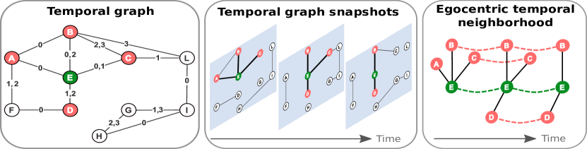
Figure 2: The left panel shows a temporal graph $\mathcal{G}$ focused on a node $E$. The middle panel shows three graph snapshots, and the right panel shows a $k=2$ order ETN for $E$ built from the sequence of its egocentric neighborhoods.

Definition 5 (Temporal graph)

A temporal graph $\mathcal{G}=(V,E)$ is a pair of sets where $V$ is a set of vertices or nodes and $E$ is a set of temporal edges, i.e., edges enriched with temporal information. Each temporal edge $e\in E$ is a quadruple $(u,v,t_{start},t_{end})$, where $u$ and $v$ are nodes ($u,v\in V$) and $t_{start}$ and $t_{end}$ are time instants representing, respectively, the beginning and the end of the interaction between node $u$ and node $v$. Given a temporal graph $\mathcal{G}$, its corresponding (static) aggregate graph $G$ is obtained removing temporal information from the edges of $\mathcal{G}$.

Definition 6 (Temporal graph snapshot)

Given a temporal graph $\mathcal{G}=(V,E)$ and a temporal gap $\Delta t$, a temporal graph snapshot at time $t$ is a static graph $G_{t}=(V_{t},E_{t})$ such that $V_{t}=V$ and there is a static edge $(u,v)\in E_{t}$ if and only if the corresponding temporal interaction $(u,v,t_{start},t_{end})\in E$ exists within $\Delta t$, i.e. $t_{start}\in[t,t+\Delta t)\lor t_{end}\in[t,t+\Delta t)$.

A temporal graph $\mathcal{G}=(V,E)$ can be represented as a sequence of temporal graph snapshots $G_{t_{1}},G_{t_{2}},...,G_{t_{m}}$ where $t_{1}$ is the smallest $t_{start}$ in $E$, $t_{i+1}=t_{i}+\Delta t$ and $t_{m}$ is smaller than the largest $t_{end}$ in $E$.

4 Mining egocentric temporal motifs

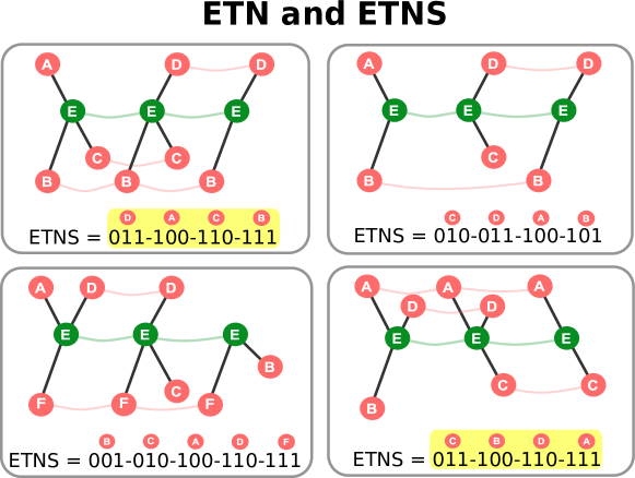
Figure 3: Examples of ETN and ETNS for different temporal graphs with $k=2$. The two highlighted ETNS are identical and correspond to isomorphic ETN.

Let us start by introducing the notions of egocentric neighborhood and egocentric temporal neighborhood.

Definition 7 (Egocentric neighborhood)

Given a (static) graph $G=(V,E)$ and a node $v\in V$, the egocentric neighborhood of $v$ is the subgraph $G(v)$ obtained by taking the neighborhood of $v$ and removing all edges not including $v$ as one of the nodes.

Note that this simple variant of the node neighborhood focuses the attention on the central node, dropping all information not related to it. We next show how to extend this egocentric focus to the temporal aspect, by following the temporal evolution of the node neighborhood.

Definition 8 (Egocentric temporal neighborhood – ETN)

Given a temporal graph $\mathcal{G}=(V,E)$, a temporal gap $\Delta t$, a temporal neighborhood order $k$ and a node $v\in V$, the egocentric temporal neighborhood of $v$ is defined as follows. Let $G_{t_{1}},G_{t_{2}},...,G_{t_{m}}$ be the sequence of temporal graphs’ snapshots for $\mathcal{G}$ with gap $\Delta t$. Let $G_{t_{1}}(v),G_{t_{2}}(v),\dots,G_{t_{m}}(v)$ be the sequence of egocentric neighborhoods of $v$ for such temporal graph snapshots. The $k$-th order egocentric temporal neighborhood of $v$ at time $t_{i}$ is a graph obtained taking $G_{t_{i}}(v),\dots,G_{t_{i+k}}(v)$ and connecting each node to the next occurrence of the same node (if any) along the sequence. In addition, each node is labelled with its position in the sequence. We refer to this graph as $G_{t_{i}}^{k}(v)$.

Figure 2 shows the extraction of an ETN from a temporal graph. The structure of ETN graphs allows to efficiently compute graph isomorphism via a graph signature. To simplify the presentation of the signature generation algorithm, we assume a function id that applied to a node in an ETN returns its identifier in the original temporal graph $\mathcal{G}$ (the letters in Figure 2).

Definition 9 (Egocentric temporal neighborhood signature (ETNS))

Given a temporal graph $\mathcal{G}=(V,E)$ and an egocentric temporal neighborhood graph $G_{t}^{k}(v)$ for node $v$, time $t$ and order $k$, an egocentric temporal neighborhood signature $s_{t}^{k}(v)$ is a bit vector encoding $G_{t}^{k}(v)$. Two egocentric temporal neighborhoods $G_{t}^{k}(v)$ and $G_{t^{\prime}}^{k}(v^{\prime})$ have the same signature if and only if they are isomorphic.

The procedure computing the ETNS for a given ETN graph is shown in Algorithm 1. The algorithm starts by initializing the signature $s$ to an empty vector and collecting all nodes of the ETN graph with distinct identifiers into a set $V$. Here $V_{t+i}(v)$ indicates the set of nodes in the $t+i$ temporal slice of $G_{t}^{k}(v)$, and the union discards duplicates according to id. For each node $u$, with the exception of the central node $v$, the algorithm then computes a bit vector encoding $s_{u}$. The encoding has length $k$ and contains at each position $i$ a Boolean flag stating whether the node (represented by its identifier id) is present in the corresponding temporal slice, i.e., $u\in V_{t+i}(v)$. After computing this bit vector, the algorithm appends it to $s$. Finally, the list of neighborhood node signatures is sorted in lexicographic order and concatenated into the final signature. Figure 3 shows some examples of ETN and corresponding ETNS for $k=2$.

procedure computeETNS($G_{t}^{k}(v)$)

     $s\leftarrow[\,]$

     $V\leftarrow\bigcup\limits_{i=0}^{k}V_{t+i}(v)$

     for $u\in V$ do

         if $u\neq v$ then

              $s_{u}\leftarrow[\,]$

              for $i=0,..,k$ do

                  if $u\in V_{t+i}(v)$ then

                       append($s_{u},1$)

                  else

                       append($s_{u},0$)                                          append($s,s_{u}$)      

     $s\leftarrow$ sort($s$)

     return flatten($s$)

Algorithm 1 Procedure for computing the signature of an ETN graph.

Theorem 1 (Isomorphic ETN)

Given two egocentric temporal neighborhoods $G_{t}^{k}(v)$ and $G_{t^{\prime}}^{k}(v^{\prime})$, Algorithm 1 returns the same signature if and only if they are isomorphic.

Proof 1

We first show that if two ETNs are isomorphic they have the same signature. Let $\pi$ be a bijection for the two ETNs as from Definition 2. Note that this bijection will map central nodes to central nodes (they are the only ones that can have a degree larger than one on a given temporal slice). By specifying a mapping between nodes, $\pi$ also implicitly defines a mapping between node identifiers. The edge-preserving property of $\pi$ implies that the mapping of identifiers is consistent (if two non-central nodes share an edge they have the same identifier). It also implies that the two paired node identifiers share the same set of edges, and thus have the same encoding. Having the same encodings for each pair of node identifiers, the resulting signatures are also the same. This concludes the first part of the proof.

We next show that if the signatures are the same the ETNs are isomorphic. We prove this by showing how to create the bijection function $\pi$. Recall that a signature is a flattened sorted list of encodings of node identifiers, and that all encodings have the same length $k+1$. We start by pairing node identifiers in the two graphs by their positions in the respective signatures. We then map nodes with paired identifiers by matching their node labels (i.e., positions in the underlying graph sequence). Given that the node encodings of the paired identifiers are the same, the corresponding nodes appear in the same positions in the underlying sequence (thus matching by node labels produces a perfect match). We repeat the same matching for the only unpaired node identifiers, which correspond to the central node. Note that by definition of ETN the central node appears with all labels from 1 to $k+1$. Being redundant we omit its encoding from the signature. By construction, mapped nodes share the same label, i.e., $\ell(u)=\ell(\pi(u))$ for all $u$. Concerning edges, by definition of ETN edges are only between the central node and the neighbors, and between consecutive instances of the same node along the sequence. The former requirement is easily satisfied as each (non-central) node is always connected to the central node having the same label. The latter is satisfied because by construction if two node identifiers have the same encoding their corresponding nodes have the same edges (recall that central nodes have the same encoding even if it is not part of the signature). This concludes the proof.

We are now ready to introduce the algorithm for extracting statistics on ETNs from a temporal graph. The pseudocode of the algorithm is shown in Algorithm 2.

procedure countETN($\mathcal{G}$,$\Delta t$,$k$)

     ${\cal S}\leftarrow\emptyset$

     $G_{t_{1},..,t_{m}}\leftarrow$ ExtractSnapshots($\mathcal{G}$,$\Delta t$)

     for $i=1,..,m-k$ do

         for $v\in V_{t_{i}}$ do

              $G_{t_{i}}^{k}(v)\leftarrow$ buildETN($G_{t_{i}}(v),\dots,G_{t_{i+k}}(v)$)

              $s_{t_{i}}^{k}(v)\leftarrow$ computeETNS($G_{t_{i}}^{k}(v)$)

              if $s_{t_{i}}^{k}(v)\in{\cal S}$ then

                  ${\cal S}[s_{t_{i}}^{k}(v)]\leftarrow{\cal S}[s_{t_{i}}^{k}(v)]+1$

              else

                  ${\cal S}[s_{t_{i}}^{k}(v)]\leftarrow 1$                             

     return ${\cal S}$

Algorithm 2 Procedure for extracting counts of ETN graphs from a temporal graph.

The algorithm takes as input a temporal graph $\mathcal{G}$, a temporal gap $\Delta t$ and a temporal neighborhood order $k$ and returns a dictionary of counts ${\cal S}$ mapping ETNs to the number of occurrences of the corresponding ETN in $\mathcal{G}$. It starts by initializing ${\cal S}$ to the empty set and extracting the sequence of temporal graph snapshots of $\mathcal{G}$ for gap $\Delta t$. For each time $t_{i}$ and node $v$ ($V_{t_{i}}$ is the set of nodes of graph $G_{t_{i}}$) it builds the corresponding ETN and computes its associated signature using Algorithm 1. The signature is finally used to update the ETN counts in ${\cal S}$. Note that this update step is extremely efficient thanks to the fact that ETNs are bit vectors.

Theorem 2 (Complexity of computeETNS)

The worst-case complexity of computeETNS is $\mathcal{O}(d^{(k)}\log{d^{(k)}})$, where $d^{(k)}$ is the maximal degree of the network when considering edges within a $k\cdot\Delta t$ temporal range.

Proof 2

Building the signature requires to create an encoding of length $k+1$ for each of the nodes in $G_{t_{i}}^{k}(v)$ with distinct identifier, which are $|V|$. The complexity is thus $\mathcal{O}(|V|)$. Sorting the signature requires sorting each of these encodings, which costs $\mathcal{O}(|V|\cdot\log{|V|})$. The worst case complexity can be obtained setting $|V|=d^{(k)}$, giving $\mathcal{O}(d^{(k)}\log{d^{(k)}})$.

Theorem 3 (Complexity of countETN)

The worst-case complexity of countETN is $\mathcal{O}(n\cdot m\cdot d^{(k)}\log{d^{(k)}})$, where $n$ is the number of nodes in the network, $m$ is the overall number of temporal snapshots, and $k$ and $d^{(k)}$ are as in Theorem 2. The number of temporal snapshots is computed as $m=(T_{end}-T_{start})/\Delta t$, where $T_{start}$ and $T_{end}$ are the smallest $t_{start}$ and the largest $t_{end}$ in the network respectively and $\Delta t$ is the temporal gap.

Proof 3

Note first that the procedure ExtractSnapshots is introduced to simplify the explanation, but the underlying algorithm never explicitly materializes the sequence of temporal graph snapshots for the whole network but directly extracts the ETN using buildETN. This latter procedure costs $|G_{t}^{k}(v)|$, i.e., the number of nodes in the resulting ETN, which is upper bounded by $d^{(k)}\cdot k$. The procedure is repeated $n\cdot(m-k)$ times. Computing all ETNs thus costs $\mathcal{O}(n\cdot m\cdot d^{(k)}\cdot k)$, and converting them to ETNs costs $\mathcal{O}(n\cdot m\cdot d^{(k)}\log{d^{(k)}})$. The count update can be done in constant time thanks to the fact that ETNs are bit vectors, so the overall worst-case complexity is $\mathcal{O}(n\cdot m\cdot d^{(k)}\log{d^{(k)}})$.

Note that for reasonable values of $k$ and $\Delta t$, $d^{(k)}$ is independent of the size of the network, so that the overall complexity is $\mathcal{O}(n\cdot m)$.

To extract statistically significant ETN from a temporal graph $\mathcal{G}$, we rely on the support of a null model $\bar{\mathcal{G}}$, defined as follows Holme and Saramaki (2012); Holme (2015); Jazayeri and Yang (2020):

Definition 10 (Temporal Graph Null Model)

Given a temporal graph $\mathcal{G}$, consider the temporal graph snapshot $G_{t_{1}},G_{t_{2}},\dots,G_{t_{m}}$ (Definition 6) representation of $\mathcal{G}$. The null model $\bar{\mathcal{G}}$ of $\mathcal{G}$ is obtained by randomly shuffling the snapshots $G_{t_{1}},G_{t_{2}},\dots,G_{t_{m}}$.

Hence a null model $\bar{\mathcal{G}}$ is a temporal graph with the same number of nodes, the same number of snapshots and the same number of connections between each couple of nodes but without any temporal correlation. The procedure can be repeated an arbitrary number of times to produce a set of null models that the original temporal graph can be compared with.
As will be shown in the experimental evaluation, this allows to identify non-trivial temporal structures in a much more selective way with respect to alternative non-egocentric mining approaches.

Finally, we define the Egocentric Temporal Motifs (ETM) as follows:

Definition 11 (Egocentric Temporal Motifs (ETM))

Given a temporal graph $\mathcal{G}$, $n$ null models $\bar{\mathcal{G}}$, and the parameters $\alpha$ (over-representation), $\beta$ (minimum deviation) and $\gamma$ (minimum frequency) appearing in Definition 4, the set of ETMs for $\mathcal{G}$ is obtained applying Definition 4 to $\mathcal{G}$ where sub-graphs are represented by the set of its ETNs found according to Definition 8 for each of its nodes.

We name the algorithm extracting ETM from a temporal graph ETMM, standing for Egocentric Temporal Motif Miner.

5 ETM-based graph distance

To show the importance of the egocentric perspective in networks of social interactions, we introduce a simple metric that measures the distance between graphs in terms of their respective ETM. To do this, we first define the ETN-based embedding of a temporal graph.

Definition 12 (ETN-based embedding)

Given a temporal graph $\mathcal{G}$ and a list $M$ of ETNs, we define $EMB_{M}(\mathcal{G})$ as the embedding of $\mathcal{G}$ in a vector of cardinality $|M|$, in which the $i^{th}$ element of $EMB_{M}(\mathcal{G})$ represents the number of occurrences of $M[i]$ in $\mathcal{G}$.

Given a list of ETN, the distance between two temporal graphs is then defined as the distance between their respective ETN-based embeddings.

Definition 13 (ETN-based distance)

Given two temporal graphs $\mathcal{G}_{1}$, $\mathcal{G}_{2}$ and a list $M$ of ETNs, we define $dist_{M}(\mathcal{G}_{1},\mathcal{G}_{2})$ as the cosine distance between the ETN-based embeddings of $\mathcal{G}_{1}$ and $\mathcal{G}_{2}$:

$$dist_{M}(\mathcal{G}_{1},\mathcal{G}_{2})=1-\dfrac{EMB_{M}(\mathcal{G}_{1})\cdot EMB_{M}(\mathcal{G}_{2})}{||EMB_{M}(\mathcal{G}_{1})||\;||EMB_{M}(\mathcal{G}_{2})||}$$ (1)

where $\cdot$ is the dot product and $||\cdot||$ is the Euclidean norm.

The distance between two temporal graphs can now be computed by first extracting their respective lists of ETM, finding the set of ETM shared by the two graphs and computing their ETN-based distance using this set.

Definition 14 (ETM-based distance)

Given two temporal graphs $\mathcal{G}_{1}$, $\mathcal{G}_{2}$, two corresponding sets of $n$ null models $\bar{\mathcal{G}_{1}}$ and $\bar{\mathcal{G}_{2}}$ and three parameters $\alpha$, $\beta$ and $\gamma$, we define $dist(\mathcal{G}_{1},\mathcal{G}_{2})$ as:

$$dist(\mathcal{G}_{1},\mathcal{G}_{2})=dist_{M_{1,2}}(\mathcal{G}_{1},\mathcal{G}_{2})$$ (2)

where $M_{1,2}=M_{1}\cap M_{2}$ and $M_{1}$ (resp. $M_{2}$) is the list of ETM obtained applying Definition 11 to $\mathcal{G}_{1}$ (resp. $\mathcal{G}_{2}$).

6 Experimental setup

In the following we describe the different groups of network datasets we employed in our experiments and the non-egocentric miners and graph distances that we used as competitors.

6.1 Close proximity interaction datasets

The first group of datasets focuses on close proximity interactions, and contains three high school datasets, a work place, a hospital, a primary school and a university campus (DTU). All datasets except the university campus have been collected using the wearable sensors developed by the SocioPatterns collaboration, equipped with radio-frequency identification devices (RFIDs) capturing face-to-face interactions. The devices record an interaction if and only if there is at least one exchanged signal within 20 seconds, so 20 seconds the smallest time resolution. The DTU dataset Sapiezynski et al. (2019) instead represents proximity interactions among university students, collected over a month using Bluetooth technology to infer physical co-location. The datasets are briefly described in the following.
HighSchool11 Fournet and Barrat (2014). The dataset has been collected in 2011 in Lycée Thiers, Marseilles, France, over four days (Tuesday to Friday). It reports the interactions among 118 students and 8 teachers in three different high school classes. Number of edges: $1709$, number of nodes: $126$.
HighSchool12 Fournet and Barrat (2014). The dataset has been collected in 2012 in Lycée Thiers, Marseilles, France, over seven days (Monday to Tuesday of the following week). It reports the interactions among 180 students in five different high school classes. Number of edges: $2220$, number of nodes: $180$.
HighSchool13 Mastrandrea et al. (2015). The dataset has been collected in 2013 in Lycée Thiers, Marseilles, France, over five days in December. It reports the interactions among 327 students in nine different high school classes. Number of edges: $5818$, number of nodes: $327$.
InVS13 Génois et al. (2015). The dataset has been collected in 2013 at the Institut National de Veille Sanitaire, a health research institute near Paris, over two weeks. The dataset contains 92 individuals divided in five departments: DISQ, DMCT, SFLE, DSE and SRH. Number of edges: $755$, number of nodes: $92$.
LH10 Vanhems et al. (2013). The dataset has been collected in the geriatric ward of a university hospital Vanhems et al. (2011) in Lyon, France, over four days in December 2010. The individuals belong to four classes: medical doctors (MED), paramedical staff (NUR), administrative staff (ADM) and patients (PAT). Number of edges: $1139$, number of nodes: $75$.
Primary school Stehlé et al. (2011). The dataset has been collected in a primary school in France, over two days in October 2009. The individuals belong to two classes: teachers (10 individuals) and children (232 individuals). Number of edges: $8317$, number of nodes: $242$.
DTU Sapiezynski et al. (2019). The dataset represents the interactions among university freshmen students in the Copenhagen University. In particular, DTU represents the network of interactions among students collected over a month using Bluetooth technology to infer physical proximity. Number of edges: $79530$, number of nodes: $692$.

6.2 Distance communication datasets

The second group of datasets contains distance interactions with different communication technologies, namely phone calls, SMSs and emails. The idea is to check whether ETMs are capable of distinguishing graphs according to the underlying communication technology. The datasets are briefly described in the following.
DTU calls Sapiezynski et al. (2019). The dataset represents phone calls among university freshmen students in the Copenhagen University. Number of edges: $605$, number of nodes: $525$.
Friends and Family calls Aharony et al. (2011). The dataset represents phone calls among members of a young-family residential living community adjacent to a major research university in North America. Number of edges: $432$, number of nodes: $129$.
DTU SMS Sapiezynski et al. (2019). The dataset represents SMSs among university freshmen students in the Copenhagen University. Number of edges: $697$, number of nodes: $568$.
Friends and Family SMS Aharony et al. (2011). The dataset represents SMSs among members of a young-family residential living community adjacent to a major research university in North America. Number of edges: $153$, number of nodes: $85$.
Email EU Paranjape et al. (2017) The dataset is a collection of emails between members of a European research institution. Number of edges: $16064$, number of nodes: $986$.
Email DNC Rossi and Ahmed (2015) The dataset is a collection of leaked emails between members of the 2016 Democratic National Committee. Number of edges: $16064$, number of nodes: $986$.

6.3 Synthetic datasets

The last group of datasets consists in synthetic temporal networks, and aims at checking whether ETMs retain information concerning (temporal variants of) popular network topologies. Each network is built as a temporal graph where the first timestamp is a static synthetic network suitably generated, while the following temporal layers are recursively generated imposing a fixed correlation with the previous ones. In details, the timestamp $n+1$ is obtained by randomly swapping a fixed fraction $f$ of couples of edges present in the network at timestamp $n$. In this way the temporal network that we obtain is characterized by a realistic temporal correlation between timestamps and each static network has the same degree distribution. We chose $f=0.3$ and we used as initial static networks six different graphs: two Erdős-Rényi Erdős and Rényi (1960) networks (with $p=0.01$ and $p=0.001$), two scale-free networks Barabási and Albert (1999) (with the same parameters $\alpha=0.41$, $\beta=0.54$, $\gamma=0.05$, $\delta_{in}=0.2$, $\delta_{out}=0$ of the algorithm described in Bollobás et al. (2003) but with two different random seeds), and two small-world networks Watts and Strogatz (1998) (with $p=2$ and $p=8$, but $k=3$ for both). Table 1 shows the parameters of the generated graphs.

Name	# nodes	# edges	Time stamps
Erdos Renyi (p=0.01)	64	1610	301
Erdos Renyi (p=0.001)	13	78	301
Scale Free (G1)	100	2748	301
Scale Free (G2)	100	3524	301
Small World (p=2)	100	4581	301
Small World (p=8)	100	4340	301

Table 1: Synthetic temporal graphs parameters

6.4 Non-egocentric miners

As previously stated, no alternative approaches exist that focus on mining egocentric temporal motifs. However, to provide some comparative evaluation for the results of our mining algorithm, we also ran the state of the art non-egocentric temporal motif mining algorithm by Paranjape et al. Paranjape et al. (2017). Note however that the motifs found by this method are prototypical of what any non-egocentric mining approach can produce. As mentioned in the related work, the method can be described as follows: $(i)$ obtain the aggregate graph of the input temporal graph (see Definition 5); $(ii)$ extract (static) $n$-node $l$-edges motifs, where $n$ is the number of nodes in the motif and $l$ is the number of edges (parameters of the algorithm), using standard approaches for determining motifs (where the null models have the same aggregate degree distribution of the input graph); and $(iii)$ for each static motif count its isomorphic sub-graphs on the temporal network, i.e. with edges possibly appearing at different times. If the maximum distance in time among the different edges is less than a given time $\delta$, the sub-graph is denoted as a temporal motif. In the following, we refer to the Paranjape et al. Paranjape et al. (2017) method as TMM.

6.5 Non-egocentric graph distances

In this subsection, we present four distances based on micro-scale, meso-scale and global features of the temporal graph.
NetSimile: Berlingerio et al. Berlingerio et al. (2012) developed NetSimile, a tool for network distance. This method relies on a set of seven features of the network’s nodes. Such features are: degree of the nodes, clustering coefficient, average number or nodes in two-hop neighborhood, average clustering coefficients of the neighbors of a node, number of edges in the node egonet (induced sub-graph of node and neighbors), number of outgoing edges and number of neighbors of the ego. First, the median, mean, standard deviation, skewness, and kurtosis are computed for each feature, producing a graph embedding of $7\times 5=35$ elements. Then, the distance among graphs is computed as the Canberra distance between their respective embeddings.
To apply such method to the aforementioned datasets, we compute the aggregated network, that is, the network obtained by removing the temporal dimension in the input data and the duplicated edges.
Modified NetSimile: NetSimile is not originally conceived for temporal graphs. We thus considered a variant of the method that includes the number of temporal interactions of a node as an additional feature over which to compute the statistics, thus producing an embedding of dimension $40$.
Weighted Laplacian: While previous distances rely on local features of the input graph, the Weighted Laplacian leverages global features. First of all, a weighted aggregated static graph is created, in which the weights on an edge represent the number of interactions (over time) that the edge has had. Then the Laplacian matrix is defined as $L=D-W$, where $D$ is the degree matrix and $W$ is the matrix of edge weights.
To compute the distance among two temporal graphs $\mathcal{G}_{1}$ and $\mathcal{G}_{2}$, we calculate the Laplacian matrices $L_{1}$ and $L_{2}$, then we set $k$ equal to the minimum number of nodes between $\mathcal{G}_{1}$ and $\mathcal{G}_{2}$, and finally we compute the Euclidean distance between the first $k$ eigenvalues of $L_{1}$ and $L_{2}$.
Temporal motifs: To compute the distance between networks using meso-scale features, we considered a distance induced by (non-egocentric) temporal motifs. This is achieved by applying a variant of Definition 14 that uses temporal motifs as discussed in Section 6.4 in place of ETM.

7 Results

We start by showing qualitative results in which we compare egocentric and non-egocentric motifs, and then report a quantitative analysis of the effectiveness of our ETM-based graph distance as compared to alternative non-egocentric graph distance measures.

7.1 Egocentric vs non-egocentric temporal motifs

We compare motifs found by our ETMM with those generated by TMM. We set the number of temporal steps $k=2$ for ETMM, while for TMM we consider $3$-nodes and $3$-edges structures. These values allow to generate non-trivial motifs and to find a significant amount of them in each dataset. As will be clear in the next, the difference between the methods is evident and does not depend on the specific choice for these parameters. Note that ETMM does not require to set the number of nodes and edges and it can in principle extract motifs with an arbitrary number of neighbors. Following Milo et al. Milo et al. (2002) we set the number of null models $n=100$, with parameters $\alpha=0.01$, $\beta=0.1$ and $\gamma=5$.

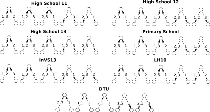
Figure 4: Most frequent temporal motifs discovered by TMM on the seven networks for $\Delta t=300$.

To give an insight of the main differences between egocentric and non-egocentric motifs and highlight the usefulness of the former in discovering patterns of social interaction, we report the five most frequent motifs found by the different methods. We focus on a temporal gap $\Delta t=300$ seconds, but results are quite similar for different temporal gaps.

Figure 4 shows the first five motifs found by TMM on the different datasets, ordered by frequency. These motifs show some dynamics in the interaction, but it is difficult to interpret them in terms of social interaction patterns or to identify some clear features that distinguish the various datasets. Moreover, Figure 4 shows that the five most frequent motifs are the same for all the datasets, with the only exception of the fifth motifs of InVS13 and LH10.

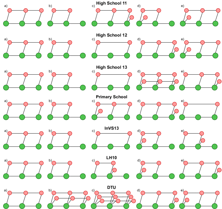
Figure 5: Most frequent egocentric temporal motifs discovered by ETMM on the three datasets for $\Delta t=300$.

The five most frequent motifs discovered by our method are reported in Figure 5. Note that the egocentric focus allows to generate motifs which are quite interpretable in terms of social interactions of the person under investigation (the ego). For instance, for HighSchool11 (first line) we identify a continuous interaction with another person (a) (c) (e), possibly combined with a third person joining at the beginning (e) or at the end (c) of the interaction.

Concerning the other datasets, even if the first two ETMs are the same (except for the DTU dataset), our approach does identify some differences that can be related to the different type of networks under investigation. For example, our method is able to identify motifs characterized by rich and dynamic interactions among students in high school and university, and by sparse and short interactions among employees in the research institute. The last line of Figure 5 shows the motifs found by ETMM on the DTU dataset, and it is easy to see that the structures of the discovered motifs are quite different and more complex with respect to the structures of the motifs found in the other datasets. This may also depend on the fact that the DTU dataset, collected using Bluetooth technology, captures co-location and not face-to-face interactions.

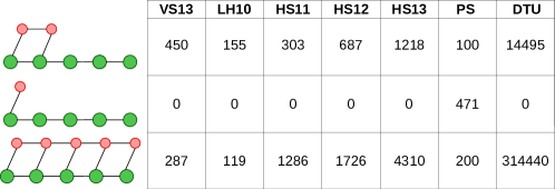
Figure 6: The figure shows the frequencies of three ETM for each dataset. The ETMs are those with the maximum variance among datasets.

To provide further insights on the relationship between motifs and types of networks, we looked for the set of temporal motifs that most discriminates among different datasets. We selected the three egocentric temporal motifs with maximum variance of occurrence among the datasets, and report their frequencies in Figure 6. The difference between the primary school and the other datasets is striking. The former contains a motif that is totally missing in the other networks, namely the case where an individual briefly interacts with another one (for less than 5 minutes) and has no more interactions in the following 20 minutes. This small set of motifs may seem a poor description of the analyzed social settings. However, it is surprisingly accurate in catching differences and similarities among datasets, as we will see in next section.

7.2 Egocentric vs non-egocentric graph distances

To give some quantitative estimate of the descriptiveness of the motifs found by our method, we study their effectiveness in measuring the distance among the networks described in Section 6. In particular, we show the importance of the egocentric perspective in identifying similar social contexts by means of network distances (Definition 14).

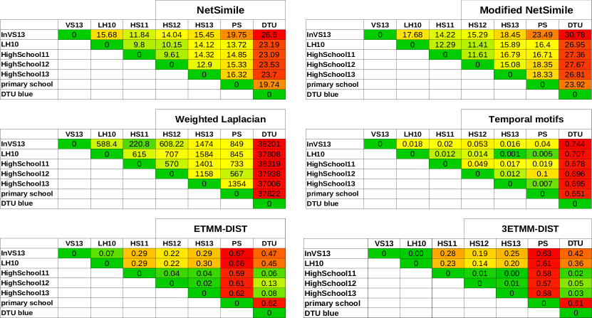
Figure 7: Distances among networks using five different methods, namely: NetSimile, Modified NetSimile, Weighted Laplacian, Temporal motifs and ETM-based distance. Each element of the table is colored in a color scale from green (minimum distance) to red (maximum distance). The last tables show the distances obtained using ETM-based distance using $\Delta t=300$ and $k=4$, with all motifs (left) and the three most discriminative ones (right).

Figure 7 shows the distances computed with the four non-egocentric methods reported in Section 6.5 (first two rows) and with our ETM-based distance (last row). Each table reports the pairwise distances between networks and each element is colored with a color scale starting from green (minimum distance) to red (maximum distance). The figure clearly shows that all non-egocentric methods have serious problems in producing meaningful distances between interaction networks. First, all of them consider DTU to be the farthest away from all other networks. However, we expect that DTU network, which collects the co-location behaviors of university students, should show some similarities with the ones capturing the face-to-face interactions of high school students, namely HighSchool11, HighSchool12 and HighSchool13. These similarities seem not adequately detected by these methods. As previously anticipated, the fact that DTU results appear so different from those obtained with the other datasets may depend on the fact that different technologies (RFID vs Bluetooth) have been used to collect the data, suggesting that non-egocentric approaches fail in revealing social patterns when different technologies are at place. We also notice that both NetSimile and Modified NetSimile (first row) detect hospital (LH10) as the closest network to primary school; this appears as an unexpected result, considering the differences between these two social contexts. Moreover, the Weighted Laplacian method (first table second row) fails in identifying similar environments, since we observe that InVS13 is very close to HighSchool11 but quite distant from HighSchoo13. Finally, according to (non-egocentric) temporal motifs (second table second row) the network LH10 is very close to almost all datasets, being almost identical to HighSchool13.

The last row of Figure 7 shows the results of our ETM-based distance (for $\Delta t=300$ and $k=4$), using all ETMs (left) and only the three most discriminative ones (right), i.e., those maximizing the variance of ETM frequencies among datasets (shown in Figure 6). The reported network distances provide a more satisfactory description of the similarity between the underlying datasets. First of all, the three high school networks are very close to each other, with distances around 0, while presenting larger distances with all other networks. Moreover, among the other networks, the closest one is represented by the one capturing the co-location behavior of university students (DTU), which are expected to share some behavioral routines with high school students (e.g., class attendance). This shows that ETM is capable of finding similar social interaction patterns despite the use of different data collection technologies, something alternative non-egocentric measures completely fail to achieve. The network which is farthest away from all the others is the primary school network: this may be explained by the fact that primary school children seem to experience interaction dynamics which are significantly different from the ones characterizing the social settings of young adults and adults. Finally, we observe that another sensible niche is represented by the two working places, namely the hospital and the research institute, quite similar between each other and quite distinct from all other settings. Interestingly, limiting the set of ETMs to the three most discriminative ones produces results which are very similar to those obtained with the full set of motifs (around six thousands). This is a surprising result and a confirmation of the effectiveness of the egocentric perspective in characterizing different types of social interaction settings.

7.3 Sensitivity analysis

In the following we provide a sensitivity analysis showing how the choice of the parameters, namely the temporal gap $\Delta t$ and the temporal neighborhood order $k$, affect the ETM-based distance. In Figure 8 we report the ETM-based distance among datasets using $\Delta t$ equal to $300$ and $900$ seconds, and $k$ ranging from $3$ to $5$. We observe that results are quite stable. For intermediate values of the parameters, results are very similar to those presented for $\Delta t=300$ and $k=4$, with distances that tend to increase for increasing values of $\Delta t$ and $k$. Intuitively, small values of both $\Delta t$ and $k$ (i.e., $\Delta t=300$ and $k=3$, top left matrix) produce small motifs, leading to a partial reduction in discriminative capacity, with the primary school becoming (more) similar to workplaces and high schools. On the other side, large values of both $\Delta t$ and $k$ (i.e., $\Delta t=900$ and $k=5$, bottom right matrix) determine a slight decrease in the capacity of detecting similarities among related datasets (namely between different high schools). This is again not surprising, as jointly increasing $\Delta t$ and $k$ substantially increases the required length for a temporal fragment to match a motif, making it more complex for the method to mine relevant motifs.

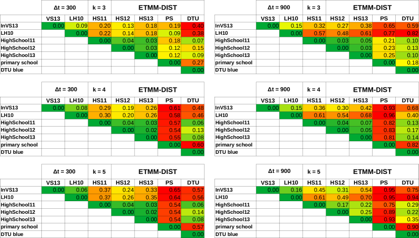
Figure 8: ETM-based distances obtained using $\Delta t=300,900$ and $k=3,4$ and $5$.

7.4 Results on distance communication and synthetic datasets

In this section we evaluate the ability of the ETM-based distance to characterize networks beyond close proximity interaction data. First of all we consider other typologies of social data representing distance communication interactions (Fig. 9), then we explore the algorithm performance on synthetic temporal graphs (Fig. 10).

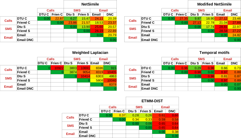
Figure 9: Distances among different communication networks using five different methods, namely: NetSimile, Modified NetSimile, Weighted Laplacian, Temporal motifs and ETM-based distance. Each element of the table is colored in a color scale from green (minimum distance) to red (maximum distance). The last table shows the distances obtained using ETM-based distance with $\Delta t=3600$ and $k=4$.

The non-physical interaction datasets that we consider employ different communication technologies (phone calls, SMSs and emails, see Section 6.2). For this experiment, we choose $k=4$ and $\Delta t=3600$, a temporal gap for which the six temporal networks are characterized by a similar average degree (equal to 0.052 for phone calls, 0.049 for SMSs and 0.051 for emails). Results are shown in Figure 9. Non-egocentric methods manage to capture the similarity among some of the networks using the same technology (e.g., SMSs for NetSimile and Modified NetSimile, emails for temporal motifs), but they badly fail in most cases. On the other hand, the ETM-based distance is quite consistent in capturing the similarity between networks employing the same communication technology. Moreover, networks based on SMSs and phone calls are more similar to each other than networks based on emails, as expected. This is a further proof of the versatility of ETM patterns to characterize temporal behaviors.

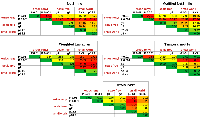
Figure 10: Distances among different synthetic networks using five different methods, namely: NetSimile, Modified NetSimile, Weighted Laplacian, Temporal motifs and ETM-based distance. Each element of the table is colored in a color scale from green (minimum distance) to red (maximum distance). The last table shows the distances obtained using ETM-based distance with $k=4$. No temporal gap is needed in this case, as the networks are not extracted from time series but synthetically generated according to the procedure described in Section 6.3.

Results for the synthetic datasets are shown in Figure 10. Our ETM-based distance is clearly capable of detecting similarities among Erdős-Rényi graphs, outperforming all competitors, and among scale-free ones, which are however modelled reasonably well by all methods. On the other hand, the ETM-based distance lags behind all competitors in detecting similarities between small-world networks. This result sheds some light on the limitations of the egocentric perspective of our method. Indeed, ETMs deliberately discard the information on connections among neighbors of the ego node (we only consider the existence of neighbors and not their mutual behavior), thus neglecting the clustering structure of the network. This explains why the synthetic small-world networks, characterized by high values of clustering coefficient, are less effectively described by our method.

8 Conclusion

In this manuscript we proposed a novel approach for mining temporal motifs based on an ego perspective. Each motif represents the evolution, during few time steps, of the set of neighbors of a specific network node. Egocentric temporal motifs present some essential characteristics that distinguish them from standard temporal motifs.

First of all, egocentric temporal motifs are simpler, at a topological level, with respect to standard temporal motifs, since they only take into account the neighboring nodes of the ego, ignoring the connections among them. This allows both to account for larger neighborhoods and to explore more in detail the temporal aspect, including duration of contacts and contemporary interactions, usually neglected in standard procedures for temporal motif mining. This is a necessary requirement when analyzing social domains like physical human interactions, where each individual can interact with multiple people at a time, with various durations.

Second, the egocentric view has substantial advantages from a computational perspective. Traditional techniques for motif mining rely on an isomorphism test for assessing if two sub-networks are equivalent or not, and this limits their applicability to mine motifs containing a handful of nodes. The focus on an ego node allows us to sidestep this problem. We show how an egocentric temporal neighborhood, which is the sub-structure representing a candidate motif, can be encoded into a bit vector in a way such that two neighborhoods have the same encoding if and only if they are isomorphic.

We made use of seven different datasets representing social interactions and applied our egocentric temporal motif miner, comparing the results with a state of the art non-egocentric temporal motif miner. Our method is shown to be more effective in terms of selectivity and quality of the extracted motifs. By visually inspecting the most frequent motifs found in each dataset, it is apparent that our method succeeds in grasping some of the peculiarities of each dataset: more rich and dynamical interactions among students in high school and university, sparser and shorter interactions for the research institute, a combination of the two in the hospital, and a different behavior at the primary school. Importantly, differences and similarities between datasets are quantified by defining a correlation measure between egocentric signatures. The results that we obtain fully reflect the social context represented by the network, especially if compared with standard non-egocentric approaches to measure temporal networks’ distance. Later, we show how the egocentric perspective is crucial for the discrimination among different communication technologies, like phone calls, SMSs and emails, and how it also allows to characterize temporal variants of popular network topologies, like Erdős-Rényi and scale-free.

The egocentric perspective surely represents an important limitation too, since we are neglecting all the second order interactions, i.e., the interactions between neighbors of an ego node. This is especially limiting in networks which are characterized by a high clustering coefficient, as shown by the suboptimal results that we achieve on small-world networks. On the other hand, this is a necessary requirement for the bit vector encoding and hence for the extreme velocity of our method (which scales linearly with the number of nodes and the timesteps of the temporal network). This allows to mine motifs covering larger structures and longer time sequences with respect to alternative solutions. Our extensive experimental results show that, even renouncing to represent second-order interactions, the proposed method is able to recognize different social settings, substantially outperforming existing alternatives.
In conclusion, we are proposing a novel efficient method to obtain temporal motifs from the node point of view. This method is not conceived to completely replace existing temporal motif mining methods, but rather to complement them in revealing a different kind of motifs. As shown in our experimental evaluation, this can be particularly useful to study social interaction networks, which could not be properly analyzed with existing approaches.

Data availability: The source code is freely available at:
https://github.com/AntonioLonga/Egocentric-Temporal-Motifs-Miner-ETMM. The datasets employed in our experiments can be downloaded at:

• http://www.sociopatterns.org (sociopattern datasets)

• https://doi.org/10.6084/m9.figshare.7267433 (DTU)

• http://realitycommons.media.mit.edu/friendsdataset.html (Friends&Family)

• http://snap.stanford.edu/data/email-Eu-core-temporal.html (Emails)

• http://networkrepository.com/email-dnc.php (Emails DNC)

References

- Aharony et al. (2011) N. Aharony, W. Pan, C. Ip, I. Khayal, and A. Pentland. Social fmri: Investigating and shaping social mechanisms in the real world. Pervasive and Mobile Computing, 7(6):643–659, 2011.
- Alon (2007) U. Alon. Network motifs: theory and experimental approaches. Nature Reviews Genetics, 8(6):450–461, 2007.
- Araujo et al. (2014) M. Araujo, S. Papadimitriou, S. Günnemann, C. Faloutsos, P. Basu, A. Swami, E. E. Papalexakis, and D. Koutra. Com2: fast automatic discovery of temporal (‘comet’) communities. In Pacific-Asia Conference on Knowledge Discovery and Data Mining, pages 271–283. Springer, 2014.
- Barabási and Albert (1999) A.-L. Barabási and R. Albert. Emergence of scaling in random networks. science, 286(5439):509–512, 1999.
- Berlingerio et al. (2012) M. Berlingerio, D. Koutra, T. Eliassi-Rad, and C. Faloutsos. Netsimile: A scalable approach to size-independent network similarity. arXiv preprint arXiv:1209.2684, 2012.
- Bollobás et al. (2003) B. Bollobás, C. Borgs, J. T. Chayes, and O. Riordan. Directed scale-free graphs. In SODA, volume 3, pages 132–139, 2003.
- Dunlavy et al. (2011) D. M. Dunlavy, T. G. Kolda, and E. Acar. Temporal link prediction using matrix and tensor factorizations. ACM Transactions on Knowledge Discovery from Data (TKDD), 5(2):1–27, 2011.
- Erdős and Rényi (1960) P. Erdős and A. Rényi. On the evolution of random graphs. Publ. Math. Inst. Hung. Acad. Sci, 5(1):17–60, 1960.
- Fournet and Barrat (2014) J. Fournet and A. Barrat. Contact patterns among high school students. PLoS ONE, 9(9):e107878, 09 2014. doi: 10.1371/journal.pone.0107878. URL http://dx.doi.org/10.1371%2Fjournal.pone.0107878.
- Génois et al. (2015) M. Génois, C. L. Vestergaard, J. Fournet, A. Panisson, I. Bonmarin, and A. Barrat. Data on face-to-face contacts in an office building suggest a low-cost vaccination strategy based on community linkers. Network Science, 3(3):326–347, 2015.
- Gurukar et al. (2015) S. Gurukar, S. Ranu, and B. Ravindran. Commit: A scalable approach to mining communication motifs from dynamic networks. In Proceedings of the 2015 ACM SIGMOD International Conference on Management of Data, pages 475–489, 2015.
- Holme (2015) P. Holme. Modern temporal network theory: a colloquium. The European Physical Journal B, 88(9):234, 2015.
- Holme and Saramaki (2012) P. Holme and J. Saramaki. Temporal networks. Physics Reports, 519(3):97–125, 2012.
- Hulovatyy et al. (2015) Y. Hulovatyy, H. Chen, and T. Milenković. Exploring the structure and function of temporal networks with dynamic graphlets. Bioinformatics, 31(12):i171–i180, 2015.
- Jazayeri and Yang (2020) A. Jazayeri and C. C. Yang. Motif discovery algorithms in static and temporal networks: A survey. arXiv preprint arXiv:2005.09721, 2020.
- Jin et al. (2007) R. Jin, S. McCallen, and E. Almaas. Trend motif: A graph mining approach for analysis of dynamic complex networks. In Seventh IEEE International Conference on Data Mining (ICDM 2007), pages 541–546. IEEE, 2007.
- Kossinets and Watts (2006) G. Kossinets and D. Watts. Empirical analysis of an evolving social network. Science, 311(5757):88–90, 2006.
- Kossinets et al. (2008) G. Kossinets, J. Kleinberg, and D. Watts. The structure of information pathways in a social communication network. In Proceedings of the 14th ACM SIGKDD international conference on Knowledge discovery and data mining, pages 435–443, 2008.
- Kostakis et al. (2017) O. Kostakis, N. Tatti, and A. Gionis. Discovering recurring activity in temporal networks. Data Mining and Knowledge Discovery, 31(6):1840–1871, 2017.
- Kosyfaki et al. (2018) C. Kosyfaki, N. Mamoulis, E. Pitoura, and P. Tsaparas. Flow motifs in interaction networks. arXiv preprint arXiv:1810.08408, 2018.
- Kovanen et al. (2011) L. Kovanen, M. Karsai, K. Kaski, J. Kertész, and J. Saramäki. Temporal motifs in time-dependent networks. Journal of Statistical Mechanics: Theory and Experiment, 2011(11):P11005, 2011.
- Leskovec et al. (2007) J. Leskovec, J. Kleinberg, and C. Faloutsos. Graph evolution: Densification and shrinking diameters. ACM transactions on Knowledge Discovery from Data (TKDD), 1(1):2–es, 2007.
- Liu et al. (2019) P. Liu, A. R. Benson, and M. Charikar. Sampling methods for counting temporal motifs. In Proceedings of the Twelfth ACM International Conference on Web Search and Data Mining, pages 294–302, 2019.
- Mastrandrea et al. (2015) R. Mastrandrea, J. Fournet, and A. Barrat. Contact patterns in a high school: a comparison between data collected using wearable sensors, contact diaries and friendship surveys. PloS one, 10(9):e0136497, 2015.
- Milgram (1967) S. Milgram. The small world problem. Psychology today, 2(1):60–67, 1967.
- Milo et al. (2002) R. Milo, S. Shen-Orr, S. Itzkovitz, N. Kashtan, D. Chklovskii, and U. Alon. Network motifs: simple building blocks of complex networks. Science, 298(5594):824–827, 2002.
- Newman (2010) M. Newman. Network: An introduction. Oxford University Press, 2010.
- Nicosia et al. (2013) V. Nicosia, J. Tang, C. Mascolo, M. Musolesi, G. Russo, and V. Latora. Graph metrics for temporal networks. In Temporal networks, pages 15–40. Springer, 2013.
- Paranjape et al. (2017) A. Paranjape, A. R. Benson, and J. Leskovec. Motifs in temporal networks. In Proceedings of the Tenth ACM International Conference on Web Search and Data Mining, pages 601–610, 2017.
- Ray et al. (2014) A. Ray, L. Holder, and S. Choudhury. Frequent subgraph discovery in large attributed streaming graphs. In Proceedings of the 3rd International Workshop on Big Data, Streams and Heterogeneous Source Mining: Algorithms, Systems, Programming Models and Applications, pages 166–181, 2014.
- Rossi and Ahmed (2015) R. A. Rossi and N. K. Ahmed. The network data repository with interactive graph analytics and visualization. In AAAI, 2015. URL http://networkrepository.com.
- Rozenshtein et al. (2017) P. Rozenshtein, N. Tatti, and A. Gionis. Finding dynamic dense subgraphs. ACM Transactions on Knowledge Discovery from Data (TKDD), 11(3):1–30, 2017.
- Rozenshtein et al. (2020) P. Rozenshtein, G. Preti, A. Gionis, and Y. Velegrakis. Mining dense subgraphs with similar edges. arXiv preprint arXiv:2007.03950, 2020.
- Sapiezynski et al. (2019) P. Sapiezynski, A. Stopczynski, D. D. Lassen, and S. Lehmann. Interaction data from the copenhagen networks study. Scientific Data, 6(1):1–10, 2019.
- Stehlé et al. (2011) J. Stehlé, N. Voirin, A. Barrat, C. Cattuto, L. Isella, J.-F. Pinton, M. Quaggiotto, W. Van den Broeck, C. Régis, B. Lina, et al. High-resolution measurements of face-to-face contact patterns in a primary school. PloS one, 6(8):e23176, 2011.
- Tantipathananandh et al. (2007) C. Tantipathananandh, T. Berger-Wolf, and D. Kempe. A framework for community identification in dynamic social networks. In Proceedings of the 13th ACM SIGKDD international conference on Knowledge discovery and data mining, pages 717–726, 2007.
- Vanhems et al. (2011) P. Vanhems, N. Voirin, S. Roche, V. Escuret, C. Regis, C. Gorain, S. Pires-Cronenberger, M. Giard, B. Lina, F. Najioullah, et al. Risk of influenza-like illness in an acute health care setting during community influenza epidemics in 2004-2005, 2005-2006, and 2006-2007: a prospective study. Archives of internal medicine, 171(2):151–157, 2011.
- Vanhems et al. (2013) P. Vanhems, A. Barrat, C. Cattuto, J.-F. Pinton, N. Khanafer, C. Régis, B.-a. Kim, B. Comte, and N. Voirin. Estimating potential infection transmission routes in hospital wards using wearable proximity sensors. PloS one, 8(9):e73970, 2013.
- Wang et al. (2020) J. Wang, Y. Wang, W. Jiang, Y. Li, and K.-L. Tan. Efficient sampling algorithms for approximate temporal motif counting. In Proceedings of the 29th ACM International Conference on Information & Knowledge Management, pages 1505–1514, 2020.
- Wasserman et al. (1994) S. Wasserman, K. Faust, et al. Social network analysis: Methods and applications, volume 8. Cambridge university press, 1994.
- Watts and Strogatz (1998) D. J. Watts and S. H. Strogatz. Collective dynamics of ‘small-world’networks. nature, 393(6684):440–442, 1998.
- Zhao et al. (2010) Q. Zhao, Y. Tian, Q. He, N. Oliver, R. Jin, and W.-C. Lee. Communication motifs: a tool to characterize social communications. In Proceedings of the 19th ACM international conference on Information and knowledge management, pages 1645–1648, 2010.