Quantum-geometric perspective on spin-orbit-coupled Bose superfluids

Abstract

We employ the Bogoliubov approximation to study how the quantum geometry of the helicity states affects the superfluid properties of a spin-orbit-coupled Bose gas in continuum. In particular we derive the low-energy Bogoliubov spectrum for a plane-wave condensate in the lower helicity band and show that the geometric contributions to the sound velocity are distinguished by their linear dependences on the interaction strength, i.e., they are in sharp contrast to the conventional contribution which has a square-root dependence. We also discuss the roton instability of the plane-wave condensate against the stripe phase and determine their phase transition boundary. In addition we derive the superfluid density tensor by imposing a phase-twist on the condensate order parameter and study the relative importance of its contribution from the interband processes that is related to the quantum geometry.

I Introduction

Recent studies have shown that the quantum geometry of the Bloch states can play important roles in characterizing some of the fundamental properties of Fermi superfluids (SFs) peotta15 ; liang17 . The physical mechanism is quite clear in a multiband lattice: the geometric effects originate from the dressing of the effective mass of the SF carriers by the interband processes, which in return controls those SF properties that depend on the carrier mass. Besides the SF density/weight, the list includes the velocity of the low-energy Goldstone modes and the critical BKT temperature peotta15 ; liang17 ; iskin18a ; iskin18b ; iskin20a ; iskin20b ; julku18 ; wang20 . On the other hand the intraband processes give rise to the conventional effects. Depending on the band structure and the strength of the interparticle interactions, it has been established that the geometric effects can become sizeable and may even dominate in an isolated flat band peotta15 . Furthermore such geometric effects on Fermi SFs can be traced all the way back to the two-body problem in a multiband lattice in vacuum torma18 ; iskin21 .

Despite the growing number of recent works exposing the role of quantum geometry for the Fermi SFs, there is a lack of understanding in the bosonic counterparts which are much less studied julku21a ; julku21b ; yangnote . For instance Julku et al. have considered a weakly-interacting BEC in a flat band, and showed that the speed of sound has a linear dependence on the interaction strength and a square-root dependence on the quantum metric of the condensed Bloch state julku21a ; julku21b . They have also showed that the quantum depletion is dictated solely by the quantum geometry and the SF weight has a quantum-geometric origin.

Motivated by the success of analogous works on spin-orbit-coupled Fermi SFs iskin18a ; iskin18b ; iskin20a ; julku18 , here we investigate the SF properties of a spin-orbit-coupled Bose gas from a quantum-geometric perspective. Our work differs from the existing literature in several ways li15 ; zhai15 ; zhang16a . In particular we derive the low-energy Bogoliubov spectrum for a plane-wave condensate in the lower helicity band and identify the geometric contributions to the sound velocity. The geometric effects survive only when the single-particle Hamiltonian has a a $\sigma_{z}$ term in the pseudospin basis that is coupled with a $\sigma_{x}$ (and/or equivalently a $\sigma_{y}$) term. In contrast to the conventional contribution that has a square-root dependence on the interaction strength, we find that the geometric ones are distinguished by a linear dependence. Similar to the Fermion problem where the geometric effects dress the effective mass of the Goldstone modes, here one can also interpret the geometric terms in terms of a dressed effective mass for the Bogoliubov modes. We also discuss the roton instability of the plane-wave ground state against the stripe phase and determine the phase transition boundary. All of these results are achieved analytically by reducing the $4\times 4$ Bogoliubov Hamiltonian (that involves both lower and upper helicity bands) down to $2\times 2$ through projecting the system onto the lower helicity band. The projected Hamiltonian works extremely well except for a tiny region in momentum-space around the point where the helicity bands are degenerate. In addition we derive the SF density tensor by imposing a phase-twist on the condensate order parameter and analyze the relative importance of its contribution from the interband processes yangnote .

The rest of the paper is organized as follows. We begin with the theoretical model in Sec. II: the many-body Hamiltonian is introduced in Sec. II.1 and the noninteracting helicity spectrum is reviewed in Sec. II.2. Then we present the Bogoliubov mean-field theory for a plane-wave condensate in Sec. III: the four branches of the full Bogoliubov spectrum are discussed in Sec. III.1 and the two branches of the projected (i.e., to the lower-helicity band) Bogoliubov spectrum are derived in Sec. III.2. Furthermore, by analyzing the resultant Bogoliubov spectrum in the low-energy regime, we find closed-form analytic expressions for the Bogoliubov modes in Sec. III.3 and for the roton instability of the plane-wave condensate against the stripe phase in Sec. III.4. Finally we derive and analyze the SF density tensor and condensate density in Sec. IV. The paper ends with a summary of our conclusions given in Sec. V.

II Theoretical Model

In order to study the interplay between a BEC and SOC, and having cold-atom systems in mind, here we consider a two-component atomic Bose gas that is characterized by a weakly-repulsive zero-ranged (contact) interactions in continuum. It is customary to refer to such a two-component bosonic system as the pseudospin-$1/2$ Bose gas.

II.1 Pseudospin-$1/2$ Bose Gas

In particular, by making use of the momentum-space representation, we express the single-particle Hamiltonian in the usual form

$$\mathcal{H}_{0}=\sum_{\mathbf{k}}\Lambda_{\mathbf{k}}^{\dagger}\left[\big{(}\varepsilon_{\mathbf{k}}+\varepsilon_{\mathbf{k_{0}}}\big{)}\sigma_{0}+\frac{\mathbf{d}_{\mathbf{k}}\cdot\boldsymbol{\sigma}}{m}\right]\Lambda_{\mathbf{k}},$$ (1)

where $\mathbf{k}=(k_{x},k_{y},k_{z})$ is the momentum vector with $\hbar=1$ and $\Lambda_{\mathbf{k}}^{\dagger}=\big{(}a_{\uparrow\mathbf{k}}^{\dagger}\;a_{\downarrow\mathbf{k}}^{\dagger}\big{)}$ is a two-component spinor with the creation operator $a_{\sigma\mathbf{k}}^{\dagger}$ for a pseudospin-$\sigma$ particle in state $|\sigma\mathbf{k}\rangle=a_{\sigma\mathbf{k}}^{\dagger}|0\rangle.$ Here $\sigma=\{\uparrow,\downarrow\}$ labels the two components of the Bose gas and $|0\rangle$ is the vacuum state. The first term $\varepsilon_{\mathbf{k}}=k^{2}/(2m)$ is the kinetic energy of a particle where $\varepsilon_{\mathbf{k_{0}}}$ is a convenient choice of an energy offset ($\mathbf{k_{0}}$ is defined below) and $\sigma_{0}$ is an identity matrix. The second term is the so-called SOC where $\boldsymbol{\sigma}=(\sigma_{x},\sigma_{y},\sigma_{z})$ is a vector of Pauli spin matrices and $\mathbf{d}_{\mathbf{k}}=\big{(}d^{x}_{\mathbf{k}},d^{y}_{\mathbf{k}},d^{z}_{\mathbf{k}}\big{)}$ is the SOC field with linearly dispersing components $d^{i}_{\mathbf{k}}=\alpha_{i}k_{i}.$ Here we choose $\alpha_{i}\geq 0$ and $\alpha_{x}\geq\{\alpha_{y},\alpha_{z}\}$ without the loss of generality.

Similarly a compact way to express the intraspin and interspin interaction terms is

$$\mathcal{H}_{U}=\frac{1}{2V}\sum_{\begin{subarray}{c}\sigma\sigma^{\prime}\\ \mathbf{k_{1}}+\mathbf{k_{2}}=\mathbf{k_{3}}+\mathbf{k_{4}}\end{subarray}}U_{\sigma\sigma^{\prime}}a_{\sigma\mathbf{k_{1}}}^{\dagger}a_{\sigma^{\prime}\mathbf{k_{2}}}^{\dagger}a_{\sigma^{\prime}\mathbf{k_{3}}}a_{\sigma\mathbf{k_{4}}},$$ (2)

where $V$ is the volume and $U_{\sigma\sigma^{\prime}}\geq 0$ is the strength of the interactions. Here we consider a sufficiently weak $U_{\uparrow\downarrow}$ in order to prevent competing phases that are beyond the scope of this paper. See Sec. III.4 for a detailed account of the stability analysis. In addition we include a chemical potential term $\mathcal{H}_{\mu}=-\sum_{\sigma\mathbf{k}}\mu_{\sigma}a_{\sigma\mathbf{k}}^{\dagger}a_{\sigma\mathbf{k}}$ to the total Hamiltonian $\mathcal{H}=\mathcal{H}_{0}+\mathcal{H}_{U}+\mathcal{H}_{\mu}$ of the system, and determine $\mu_{\sigma}$ in a self-consistent fashion.

II.2 Helicity Bands

Let us first discuss the single-particle ground state. The eigenvalues of the Hamiltonian matrix shown in Eq. (1) can be written as

$$\xi_{s\mathbf{k}}=\varepsilon_{\mathbf{k}}+\varepsilon_{\mathbf{k_{0}}}+s\frac{d_{\mathbf{k}}}{m},$$ (3)

where $s=\pm$ labels, respectively, the upper and lower band and $d_{\mathbf{k}}=|\mathbf{d}_{\mathbf{k}}|$ is the magnitude of the SOC field. Therefore the single-particle (helicity) spectrum exhibits two branches due to SOC. In the pseudospin basis $|\sigma\mathbf{k}\rangle$, the corresponding eigenvectors (i.e., helicity basis) $|s\mathbf{k}\rangle=a_{s\mathbf{k}}^{\dagger}|0\rangle$ can be represented as $|+,\mathbf{k}\rangle=\begin{pmatrix}u_{\mathbf{k}}&v_{\mathbf{k}}e^{i\varphi_{\mathbf{k}}}\end{pmatrix}^{\mathrm{T}}$ for the upper and $|-,\mathbf{k}\rangle=\begin{pmatrix}-v_{\mathbf{k}}e^{-i\varphi_{\mathbf{k}}}&u_{\mathbf{k}}\end{pmatrix}^{\mathrm{T}}$ for the lower helicity band, where $u_{\mathbf{k}}=\sqrt{(d_{\mathbf{k}}+d^{z}_{\mathbf{k}})/(2d_{\mathbf{k}})},$ $v_{\mathbf{k}}=\sqrt{(d_{\mathbf{k}}-d^{z}_{\mathbf{k}})/(2d_{\mathbf{k}})},$ $\varphi_{\mathbf{k}}=\arg(d^{x}_{\mathbf{k}}+id^{y}_{\mathbf{k}}),$ and $\mathrm{T}$ denotes the transpose. Alternatively,

$$\begin{pmatrix}a_{\uparrow\mathbf{k}}\\ a_{\downarrow\mathbf{k}}\end{pmatrix}=\begin{pmatrix}u_{\mathbf{k}}&-v_{\mathbf{k}}e^{-i\varphi_{\mathbf{k}}}\\ v_{\mathbf{k}}e^{i\varphi_{\mathbf{k}}}&u_{\mathbf{k}}\end{pmatrix}\begin{pmatrix}a_{+,\mathbf{k}}\\ a_{-,\mathbf{k}}\end{pmatrix}$$

is the transformation between the annihilation operators for the pseudospin and helicity states.

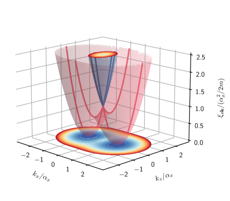
Figure 1: Helicity bands $\xi_{s\mathbf{k}}$ ( in units of $\alpha_{x}^{2}/2m$) are shown for $\alpha_{x}=2\alpha_{z}$ and $\alpha_{y}=0$ at $k_{y}=0$. The upper (red) and lower (blue) bands touch at $\mathbf{k}=\mathbf{0}$. The single-particle ground state is doubly degenerate at $\mathbf{k}=(\pm\alpha_{x},0,0)$.

For notational convenience, the lower helicity state $|-,\mathbf{k}\rangle$ is denoted as $|\phi_{\mathbf{k}}\rangle$ in the rest of the paper. Then the single-particle ground state $|\phi_{\mathbf{k_{0}}}\rangle$ is determined by setting $\partial\xi_{-,\mathbf{k}}/\partial k_{i}=0,$ leading to either $k_{i}=0$ or $\alpha_{i}^{2}=d_{\mathbf{k}}$. Here we choose $\mathbf{k_{0}}=(\alpha_{x},0,0)$ without the loss of generality cui13 ; ozawa12 ; baym14 , for which case the single-particle ground-state energy $\xi_{-,\mathbf{k_{0}}}=0$ vanishes (see Fig. 1) and the single-particle ground state $|\phi_{\mathbf{k_{0}}}\rangle=\begin{pmatrix}-1/\sqrt{2}&1/\sqrt{2}\end{pmatrix}^{\mathrm{T}}$ admits a real representation. Note that the ground state is at least two-fold degenerate with the opposite-momentum state $|\phi_{-\mathbf{k_{0}}}\rangle=\begin{pmatrix}1/\sqrt{2}&1/\sqrt{2}\end{pmatrix}^{\mathrm{T}},$ and we highlight its competing role in Sec. III.4. Having introduced the theoretical model, and discussed its single-particle ground state, next we analyze the many-body ground state within the Bogoliubov mean-field approximation.

III Bogoliubov Theory

Under the Bogoliubov mean-field approximation, the many-body ground state is known to be either a plane-wave condensate or a stripe phase depending on the relative strengths between the intraspin and interspin interactions cui13 ; ozawa12 ; baym14 ; wang10 ; barnett12 . See Sec. III.4 for a detailed account of the stability analysis. Assuming that $U_{\uparrow\downarrow}$ is sufficiently weak, here we concentrate only on the former phase.

III.1 Bogoliubov Spectrum

In order to describe the many-body ground state $|\phi_{\mathbf{k_{0}}}\rangle$ that is macroscopically occupied by $N_{0}$ particles, we replace the annihilation and creation operators in accordance with $a_{\sigma\mathbf{k}}=\Delta_{\sigma}\sqrt{V}\delta_{\mathbf{k}\mathbf{k_{0}}}+\tilde{a}_{\sigma\mathbf{k}}.$ Here the complex field $\Delta_{\sigma}=\sqrt{n_{0}}\langle\sigma|\phi_{\mathbf{k_{0}}}\rangle$ corresponds to the mean-field order parameter for the condensate with condensate density $n_{0}=N_{0}/V$, $\delta_{ij}$ is a Kronecker-delta, and the operator $\tilde{a}_{\sigma\mathbf{k}}$ denotes the fluctuations on top of the ground state. Following the usual recipe, we neglect the third- and fourth-order fluctuation terms in the interaction Hamiltonian. Then the excitations are described by the so-called Bogoliubov Hamiltonian

$$\mathcal{H}_{\mathrm{B}} =\frac{1}{2}\sum_{\mathbf{q}}^{\prime}\Psi_{\mathbf{q}}^{\dagger}\begin{pmatrix}\mathbf{H}^{pp}_{\mathbf{q}}&\mathbf{H}^{ph}_{\mathbf{q}}\\ \mathbf{H}^{hp}_{\mathbf{q}}&\mathbf{H}^{hh}_{\mathbf{q}}\end{pmatrix}\Psi_{\mathbf{q}},$$ (4)

$$\mathbf{H}^{pp}_{\mathbf{q}} =\begin{pmatrix}K_{\uparrow\mathbf{q}}&U_{\uparrow\downarrow}\Delta_{\uparrow}\Delta_{\downarrow}^{*}\\ U_{\uparrow\downarrow}\Delta_{\uparrow}^{*}\Delta_{\downarrow}&K_{\downarrow\mathbf{q}}\end{pmatrix}+\frac{\mathbf{d}_{\mathbf{k_{0}+q}}\cdot\boldsymbol{\sigma}}{m},$$ (5)

$$\mathbf{H}^{ph}_{\mathbf{q}} =\begin{pmatrix}U_{\uparrow\uparrow}\Delta_{\uparrow}^{2}&U_{\uparrow\downarrow}\Delta_{\uparrow}\Delta_{\downarrow}\\ U_{\uparrow\downarrow}\Delta_{\uparrow}\Delta_{\downarrow}&U_{\downarrow\downarrow}\Delta_{\downarrow}^{2}\end{pmatrix},$$ (6)

where $\Psi_{\mathbf{q}}^{\dagger}=\big{(}\tilde{a}_{\uparrow,\mathbf{k_{0}+q}}^{\dagger}\;\tilde{a}_{\downarrow,\mathbf{k_{0}+q}}^{\dagger}\;\tilde{a}_{\uparrow,\mathbf{k_{0}-q}}\;\tilde{a}_{\downarrow,\mathbf{k_{0}-q}}\big{)}$ is a four-component spinor and $K_{\sigma\mathbf{q}}=\varepsilon_{\mathbf{k_{0}+q}}+\varepsilon_{\mathbf{k_{0}}}-\mu_{\sigma}+2U_{\sigma\sigma}|\Delta_{\sigma}|^{2}+U_{\uparrow\downarrow}|\Delta_{-\sigma}|^{2}$ with the index $-\sigma$ denoting the opposite component of the spin. The other terms are simply related via $\mathbf{H}^{hh}_{\mathbf{q}}=(\mathbf{H}^{pp}_{-\mathbf{q}})^{*}$ and $\mathbf{H}^{hp}_{\mathbf{q}}=(\mathbf{H}^{ph}_{\mathbf{q}})^{\dagger}.$ The prime symbol indicates that the summation is over all of the non-condensed states. In this approximation, $\mu_{\sigma}$ is determined by setting the first-order fluctuation terms to $0$, leading to $\mu_{\sigma}=U_{\sigma\sigma}|\Delta_{\sigma}|^{2}+U_{\uparrow\downarrow}|\Delta_{-\sigma}|^{2}.$ Note that $\Delta_{\uparrow}=-\Delta_{\downarrow}=-\sqrt{n_{0}/2}$ are real for our particular choice for the ground state $|\phi_{\mathbf{k_{0}}}\rangle$.

The Bogoliubov spectrum $E_{s\mathbf{q}}^{n}$ is determined by the eigenvalues of $\tau_{z}\mathbf{H}_{\mathbf{q}}$ julku21a ; julku21b , i.e.,

$$\tau_{z}\mathbf{H}_{\mathbf{q}}|\chi_{s\mathbf{q}}^{n}\rangle=E_{s\mathbf{q}}^{n}|\chi_{s\mathbf{q}}^{n}\rangle,$$ (7)

where $\tau_{z}$ is a Pauli matrix acting only on the particle-hole sector, $\mathbf{H}_{\mathbf{q}}$ is the $4\times 4$ Hamiltonian matrix shown in Eq. (4), and $|\chi_{s\mathbf{q}}^{n}\rangle$ is the corresponding Bogoliubov state. Here $n=\pm$ labels, respectively, the upper and lower Bogoliubov band, and $s=\pm$ labels, respectively, the quasiparticle and quasihole branch for a given band $n$, leading to four Bogoliubov modes for a given $\mathbf{q}$. The Bogoliubov states are normalized in the usual way, i.e., if we denote $|\chi_{s\mathbf{q}}^{n}\rangle=\begin{pmatrix}|\chi_{s\mathbf{q}}^{n}\rangle_{1}\\ |\chi_{s\mathbf{q}}^{n}\rangle_{2}\end{pmatrix}$ then ${{}_{1}\langle}\chi_{s\mathbf{q}}^{n}|\chi_{s\mathbf{q}}^{n}\rangle_{1}-{{}_{2}\langle}\chi_{s\mathbf{q}}^{n}|\chi_{s\mathbf{q}}^{n}\rangle_{2}=s.$ While the Bogoliubov spectrum exhibits $E_{s\mathbf{q}}^{n}=-E_{-s,-\mathbf{q}}^{n}$ as a manifestation of the quasiparticle-quasihole symmetry, Eq. (7) does not allow for a closed-form analytic solution in general, and its characterization requires a fully numerical procedure.

In order to gain some analytical insight into the low-energy Bogoliubov modes, we assume that the energy gap between the lower and upper helicity bands nearby the ground state $|\phi_{\mathbf{k_{0}}}\rangle$ is much larger than the interaction energy. This occurs when the SOC energy scale is much stronger than the interaction energy scale. In this case the occupation of the upper band is negligible, and the system can be projected solely to the lower band as discussed next.

III.2 Projected System

The total Hamiltonian $\mathcal{H}$ of the system can be projected to the lower helicity band as follows cui13 . Using the identity operator $\sigma_{0}=\sum_{s}|s\mathbf{k}\rangle\langle s\mathbf{k}|$ for a given $\mathbf{k}$, we first reexpress $a_{\sigma\mathbf{k}}=\sum_{s}\langle\sigma|s\mathbf{k}\rangle a_{s\mathbf{k}},$ and discard those terms that involve the upper band, i.e., $a_{\sigma\mathbf{k}}\to\langle\sigma|\phi_{\mathbf{k}}\rangle a_{-,\mathbf{k}}.$ This procedure leads to

$$h_{0}+h_{\mu}=\sum_{\mathbf{k}}\big{(}\xi_{-,\mathbf{k}}-\mu\big{)}a_{-,\mathbf{k}}^{\dagger}a_{-,\mathbf{k}},$$ (8)

$$h_{U}=\frac{1}{2V}\sum_{\mathbf{k_{1}}+\mathbf{k_{2}}=\mathbf{k_{3}}+\mathbf{k_{4}}}f_{\mathbf{k_{1}}\mathbf{k_{2}}}^{\mathbf{k_{3}}\mathbf{k_{4}}}a_{-,\mathbf{k_{1}}}^{\dagger}a_{-,\mathbf{k_{2}}}^{\dagger}a_{-,\mathbf{k_{3}}}a_{-,\mathbf{k_{4}}},$$ (9)

$$f_{\mathbf{k_{1}}\mathbf{k_{2}}}^{\mathbf{k_{3}}\mathbf{k_{4}}}=\sum_{\sigma\sigma^{\prime}}U_{\sigma\sigma^{\prime}}\langle\phi_{\mathbf{k_{1}}}|\sigma\rangle\langle\phi_{\mathbf{k_{2}}}|\sigma^{\prime}\rangle\langle\sigma^{\prime}|\phi_{\mathbf{k_{3}}}\rangle\langle\sigma|\phi_{\mathbf{k_{4}}}\rangle,$$ (10)

where $\mu=(\mu_{\uparrow}+\mu_{\downarrow})/2$ is the effective chemical potential and $f_{\mathbf{k_{1}}\mathbf{k_{2}}}^{\mathbf{k_{3}}\mathbf{k_{4}}}=U_{\uparrow\uparrow}v_{\mathbf{k_{1}}}v_{\mathbf{k_{2}}}v_{\mathbf{k_{3}}}v_{\mathbf{k_{4}}}e^{i(\varphi_{\mathbf{k_{1}}}+\varphi_{\mathbf{k_{2}}}-\varphi_{\mathbf{k_{3}}}-\varphi_{\mathbf{k_{4}}})}+U_{\downarrow\downarrow}u_{\mathbf{k_{1}}}u_{\mathbf{k_{2}}}u_{\mathbf{k_{3}}}u_{\mathbf{k_{4}}}+U_{\uparrow\downarrow}v_{\mathbf{k_{1}}}u_{\mathbf{k_{2}}}u_{\mathbf{k_{3}}}v_{\mathbf{k_{4}}}e^{i(\varphi_{\mathbf{k_{1}}}-\varphi_{\mathbf{k_{4}}})}$ is the effective long-range interaction for the projected system. We note that the long-range nature of the effective interaction plays a crucial role in the Bogoliubov spectrum as discussed in Sec. III.4.

Under the Bogoliubov mean-field approximation that is used in Sec. III.1, we replace the creation and annihilation operators in accordance with $a_{-,\mathbf{k}}=\sqrt{N_{0}}\delta_{\mathbf{k}\mathbf{k_{0}}}+\tilde{a}_{-,\mathbf{k}}$ and set the first-order fluctuation terms to $0$. This leads to $\mu=n_{0}f_{\mathbf{k_{0}}\mathbf{k_{0}}}^{\mathbf{k_{0}}\mathbf{k_{0}}}=(n_{0}/4)\sum_{\sigma\sigma^{\prime}}U_{\sigma\sigma^{\prime}},$ which is consistent with $\mu_{\sigma}$ that is found in Sec. III.1. The zeroth-order fluctuation terms give $-\mu N_{0}+n_{0}f_{\mathbf{k_{0}}\mathbf{k_{0}}}^{\mathbf{k_{0}}\mathbf{k_{0}}}N_{0}/2.$ Then the excitations above the ground state are described by the Bogoliubov Hamiltonian

$$h_{\mathrm{B}} =\frac{1}{2}\sum_{\mathbf{q}}^{\prime}\psi_{\mathbf{q}}^{\dagger}\begin{pmatrix}h^{pp}_{\mathbf{q}}&h^{ph}_{\mathbf{q}}\\ h^{hp}_{\mathbf{q}}&h^{hh}_{\mathbf{q}}\end{pmatrix}\psi_{\mathbf{q}},$$ (11)

$$h^{pp}_{\mathbf{q}} =\xi_{-,\mathbf{k_{0}+q}}-\mu+\frac{n_{0}}{2}\left(f_{\mathbf{k_{0}},\mathbf{k_{0}+q}}^{\mathbf{k_{0}},\mathbf{k_{0}+q}}+f_{\mathbf{k_{0}+q},\mathbf{k_{0}}}^{\mathbf{k_{0}+q},\mathbf{k_{0}}}\right.$$

$$\left.\;\;\;\;\;\;\;\;\;\;\;\;\;\;\;\;\;\;\;\;\;\;\;+f_{\mathbf{k_{0}+q},\mathbf{k_{0}}}^{\mathbf{k_{0}},\mathbf{k_{0}+q}}+f_{\mathbf{k_{0}},\mathbf{k_{0}+q}}^{\mathbf{k_{0}+q},\mathbf{k_{0}}}\right),$$ (12)

$$h^{ph}_{\mathbf{q}} =\frac{n_{0}}{2}\left(f_{\mathbf{k_{0}+q},\mathbf{k_{0}-q}}^{\mathbf{k_{0}},\mathbf{k_{0}}}+f_{\mathbf{k_{0}-q},\mathbf{k_{0}+q}}^{\mathbf{k_{0}},\mathbf{k_{0}}}\right),$$ (13)

where $\psi_{\mathbf{q}}^{\dagger}=\big{(}\tilde{a}_{-,\mathbf{k_{0}+q}}^{\dagger}\;\tilde{a}_{-,\mathbf{k_{0}-q}}\big{)}$ is a two-component spinor, and the other terms are simply related via $h^{hh}_{\mathbf{q}}=h^{pp}_{-\mathbf{q}}$ and $h^{hp}_{\mathbf{q}}=(h^{ph}_{\mathbf{q}})^{*}.$ The Bogoliubov spectrum $\epsilon_{s\mathbf{q}}$ is determined by the eigenvalues of $\tau_{z}\mathbf{h}_{\mathbf{q}}$, leading to two Bogoliubov modes for a given $\mathbf{q}$, i.e.,

$$\epsilon_{s\mathbf{q}} =\frac{h^{pp}_{\mathbf{q}}-h^{hh}_{\mathbf{q}}}{2}+s\sqrt{\left(\frac{h^{pp}_{\mathbf{q}}+h^{hh}_{\mathbf{q}}}{2}\right)^{2}-|h^{ph}_{\mathbf{q}}|^{2}},$$ (14)

$$h^{pp}_{\mathbf{q}} =\xi_{-,\mathbf{k_{0}+q}}-\mu+\frac{n_{0}}{2}\sum_{\sigma\sigma^{\prime}}U_{\sigma\sigma^{\prime}}|\langle\phi_{\mathbf{k_{0}+q}}|\sigma\rangle|^{2}$$

$$+n_{0} \sum_{\sigma\sigma^{\prime}}U_{\sigma\sigma^{\prime}}\langle\phi_{\mathbf{k_{0}+q}}|\sigma^{\prime}\rangle\langle\sigma^{\prime}|\phi_{\mathbf{k_{0}}}\rangle\langle\phi_{\mathbf{k_{0}}}|\sigma\rangle\langle\sigma|\phi_{\mathbf{k_{0}+q}}\rangle,$$ (15)

$$h^{ph}_{\mathbf{q}} =n_{0}\sum_{\sigma\sigma^{\prime}}U_{\sigma\sigma^{\prime}}\langle\phi_{\mathbf{k_{0}+q}}|\sigma\rangle\langle\sigma|\phi_{\mathbf{k_{0}}}\rangle\langle\phi_{\mathbf{k_{0}}}^{*}|\sigma^{\prime}\rangle\langle\sigma^{\prime}|\phi_{\mathbf{k_{0}-q}}^{*}\rangle.$$ (16)

Here $s=\pm$ labels, respectively, the quasiparticle and quasihole branch of the lower Bogoliubov band (i.e., $n=-$) that is discussed in Sec. III.1. See Fig. 2 for their excellent numerical benchmark except for the spurious jumps at $\mathbf{q}=\mp\mathbf{k_{0}}$ that are discussed in Sec. III.5. The Bogolibov spectrum exhibits $\epsilon_{+,\mathbf{q}}=-\epsilon_{-,-\mathbf{q}}$ as a manifestation of the quasiparticle-quasihole symmetry. Note that when $U_{\sigma\sigma^{\prime}}=U\delta_{\sigma\sigma^{\prime}}$, these expressions reduce exactly to those of Ref. julku21a ; julku21b with $M=2$, where our $h^{pp}_{\mathbf{q}}=\xi_{-,\mathbf{k_{0}+q}}+Un_{0}/2$ and $h^{ph}_{\mathbf{q}}$ correspond, respectively, to their $\mathbf{q}^{2}/(2m_{eff})+\mu$ and $\mu\alpha(\mathbf{q})$ provided that $\mu=Un_{0}/2$ in this particular case. Such a reduction may not be surprising since the intraspin interactions $U_{\uparrow\uparrow}$ and $U_{\downarrow\downarrow}$ play the roles of sublattice-dependent onsite interactions $U_{AA}$ and $U_{BB}$, and the interspin interaction $U_{\uparrow\downarrow}$ plays the role of a (long-range) inter-sublattice interaction $U_{AB}$. Thus our $U_{\sigma\sigma^{\prime}}=U\delta_{\sigma\sigma^{\prime}}$ limit corresponds precisely to the $U=U_{AA}=U_{BB}$ and $U_{AB}=0$ case that is considered in Ref. julku21a ; julku21b .

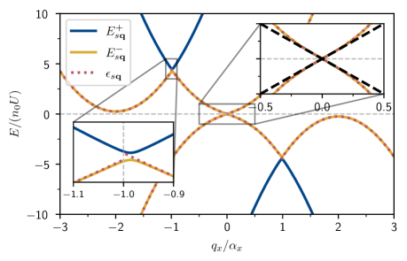
Figure 2: Bogoliubov spectrum is shown as a function of $q_{x}$ when $q_{y}=0=q_{z}$, $U=U_{\uparrow\uparrow}=2U_{\downarrow\downarrow}=4U_{\uparrow\downarrow}$, $\alpha_{x}=\alpha_{y}=2/\xi$ with the healing length $\xi=1/\sqrt{2mnU}$, and $\alpha_{z}=0$. Here the total particle density $n\approx n_{0}$ is set to $na^{3}=10^{-6}$ where $a=mU/(4\pi)$ is the scattering length. The full spectrum (solid lines) is shown together with the projected one (dotted lines) that is given by Eq. (14). In addition the low-$q$ expansion Eq. (20) is shown as dashed black lines in the right inset. If one sets $U_{\uparrow\uparrow}=U_{\downarrow\downarrow}$ then the band gap shown in the left inset disappears, i.e., see Sec. III.5 for the analysis of the spurious jumps at $q_{x}=\mp\alpha_{x}$. If one sets $U_{\uparrow\downarrow}=U_{\uparrow\uparrow}=U_{\downarrow\downarrow}$ then two additional zero-energy modes appear at $q_{x}=\mp 2\alpha_{x}$, i.e., see Sec. III.4 for the analysis of the roton instability.

We can make further analytical progress through a low-$\mathbf{q}$ expansion around the ground state, and use the fact that $|\langle\sigma|\phi_{\mathbf{k_{0}}}\rangle|^{2}=1/2$ for both pseudospin components, i.e., the $z$ component of $\mathbf{k_{0}}$ vanishes for the ground state.

III.3 Low-Momentum Expansion

Up to second order in $\mathbf{q}$, the low-energy expansions around the ground state $|\phi_{\mathbf{k_{0}}}\rangle$ can be written as

$$h^{pp}_{\mathbf{q}} =\frac{1}{2}\sum_{ij}q_{i}q_{j}M^{-1}_{ij}-\mu+\frac{n_{0}}{2}\sum_{\sigma\sigma^{\prime}}U_{\sigma\sigma^{\prime}}+2n_{0}\sum_{i\sigma\sigma^{\prime}}q_{i}U_{\sigma\sigma^{\prime}}$$

$$\times\mathrm{Re}\langle\partial_{i}\phi_{\mathbf{k}}|\sigma\rangle\langle\sigma|\phi_{\mathbf{k_{0}}}\rangle+n_{0}\sum_{ij\sigma\sigma^{\prime}}q_{i}q_{j}U_{\sigma\sigma^{\prime}}$$

$$\times\big{(}\mathrm{Re}\langle\partial_{i}\partial_{j}\phi_{\mathbf{k}}|\sigma\rangle\langle\sigma|\phi_{\mathbf{k_{0}}}\rangle+\langle\partial_{i}\phi_{\mathbf{k}}|\sigma\rangle\langle\sigma|\partial_{j}\phi_{\mathbf{k}}\rangle/2$$

$$+\langle\partial_{i}\phi_{\mathbf{k}}|\sigma^{\prime}\rangle\langle\sigma^{\prime}|\phi_{\mathbf{k_{0}}}\rangle\langle\phi_{\mathbf{k_{0}}}|\sigma\rangle\langle\sigma|\partial_{j}\phi_{\mathbf{k}}\rangle\big{)},$$ (17)

$$h^{ph}_{\mathbf{q}} =\frac{n_{0}}{4}\sum_{\sigma\sigma^{\prime}}U_{\sigma\sigma^{\prime}}+\frac{n_{0}}{2}\sum_{ij\sigma\sigma^{\prime}}q_{i}q_{j}U_{\sigma\sigma^{\prime}}\big{(}\langle\partial_{i}\partial_{j}\phi_{\mathbf{k}}|\sigma\rangle\langle\sigma|\phi_{\mathbf{k_{0}}}\rangle$$

$$-2\langle\partial_{i}\phi_{\mathbf{k}}|\sigma\rangle\langle\sigma|\phi_{\mathbf{k_{0}}}\rangle\langle\phi_{\mathbf{k_{0}}}^{*}|\sigma^{\prime}\rangle\langle\sigma^{\prime}|\partial_{j}\phi_{\mathbf{k}}^{*}\rangle\big{)},$$ (18)

where the spectrum of the lower helicity band is expanded as $\xi_{-,\mathbf{k_{0}+q}}=(1/2)\sum_{ij}q_{i}q_{j}M^{-1}_{ij}.$ Here $\mathbf{M}^{-1}$ is the inverse of the effective-mass tensor whose elements are given by $M^{-1}_{xx}=1/m$, $M^{-1}_{yy}=1/m-\alpha_{y}^{2}/(m\alpha_{x}^{2})$, $M^{-1}_{zz}=1/m-\alpha_{z}^{2}/(m\alpha_{x}^{2})$, and 0 otherwise. In addition $\mathrm{Re}$ denotes the real part of an expression and $|\partial_{i}\phi_{\mathbf{k}}\rangle$ stands for $\partial|\phi_{\mathbf{k}}\rangle/\partial k_{i}$ in the $\mathbf{k\to k_{0}}$ limit. By plugging these expansions in Eq. (14), and keeping up to second-order terms in $\mathbf{q}$, we obtain

$$\epsilon_{s\mathbf{q}} =2n_{0}\sum_{i\sigma\sigma^{\prime}}q_{i}U_{\sigma\sigma^{\prime}}\mathrm{Re}\langle\partial_{i}\phi_{\mathbf{k}}|\sigma\rangle\langle\sigma|\phi_{\mathbf{k_{0}}}\rangle+s\sqrt{X_{\mathbf{q}}},$$ (19)

$$X_{\mathbf{q}} =\mu\sum_{ij}q_{i}q_{j}\big{[}M^{-1}_{ij}+n_{0}\sum_{\sigma\sigma^{\prime}}U_{\sigma\sigma^{\prime}}\big{(}\langle\partial_{i}\phi_{\mathbf{k}}|\sigma\rangle\langle\sigma|\partial_{j}\phi_{\mathbf{k}}\rangle$$

$$+ \mathrm{Re}\langle\partial_{i}\partial_{j}\phi_{\mathbf{k}}|\sigma\rangle\langle\sigma|\phi_{\mathbf{k_{0}}}\rangle+2\langle\partial_{i}\phi_{\mathbf{k}}|\sigma^{\prime}\rangle\langle\sigma^{\prime}|\phi_{\mathbf{k_{0}}}\rangle\langle\phi_{\mathbf{k_{0}}}|\sigma\rangle$$

$$\times \langle\sigma|\partial_{j}\phi_{\mathbf{k}}\rangle+2\mathrm{Re}\langle\partial_{i}\phi_{\mathbf{k}}|\sigma^{\prime}\rangle\langle\sigma^{\prime}|\phi_{\mathbf{k_{0}}}\rangle\langle\phi_{\mathbf{k_{0}}}^{*}|\sigma\rangle\langle\sigma|\partial_{j}\phi_{\mathbf{k}}^{*}\rangle\big{)}\big{]},$$

for the low-energy Bogoliubov spectrum of the projected system. In addition to the conventional effective-mass term that depends only on the helicity spectrum, here we have the so-called geometric terms that depend also on the helicity states. The quantum geometry of the underlying Hilbert space is masked behind those terms that depend on $|\partial_{i}\phi_{\mathbf{k}}\rangle$ and $|\partial_{i}\partial_{j}\phi_{\mathbf{k}}\rangle$ julku21a ; julku21b . While most of these terms cancel one another, they lead to

$$\epsilon_{s\mathbf{q}} =n_{0}\big{(}U_{\downarrow\downarrow}-U_{\uparrow\uparrow}\big{)}\frac{\alpha_{z}q_{z}}{2\alpha_{x}^{2}}+\frac{s}{2}\sqrt{n_{0}(U_{\uparrow\uparrow}+U_{\downarrow\downarrow}+2U_{\uparrow\downarrow})}$$

$$\times \sqrt{\sum_{ij}q_{i}q_{j}M^{-1}_{ij}+n_{0}\big{(}U_{\uparrow\uparrow}+U_{\downarrow\downarrow}-2U_{\uparrow\downarrow}\big{)}\frac{\alpha_{z}^{2}q_{z}^{2}}{4\alpha_{x}^{4}}},$$ (20)

manifesting explicitly the quasiparticle-quasihole symmetry. When $U_{\uparrow\uparrow}=U_{\downarrow\downarrow}$, Eq. (20) is in full agreement with the recent literature for the reported parameters cui13 . In addition see the right inset in Fig. 2 for its numerical benchmark with Eq. (14).

Our work reveals that the linear term in $\alpha_{z}q_{z}$ that is outside of the square root as well as the quadratic term in $\alpha_{z}q_{z}$ that is in the inside have a quantum-geometric origin. Note that the geometric terms that depend on $\alpha_{x}$ and $\alpha_{y}$ vanish all together. Thus we conclude that the geometric effects survive only in the presence of a finite $\sigma_{z}$ coupling assuming a $\sigma_{x}$ (and/or equivalently a $\sigma_{y}$) coupling to begin with. See Sec. II.2 for our initial assumption in choosing $\mathbf{k_{0}}$. Although we choose a $\mathbf{k_{0}}$ that is symmetric in $y$ and $z$ directions, the condition $|\langle\sigma|\phi_{\mathbf{k_{0}}}\rangle|^{2}=1/2$ breaks this symmetry in general for other $\mathbf{k_{0}}$ values as it requires $k_{0z}=0$. The remaining geometric terms can be isolated from the conventional effective-mass term in the $\mathbf{q}\to(0,0,q_{z})$ limit when $\alpha_{z}\approx\alpha_{x}$, leading to $q_{i}q_{j}M^{-1}_{ij}=0$. Therefore this particular limit can be used to distinguish the geometric origin of sound velocity from the conventional one, i.e., unlike the conventional term that has $\propto\sqrt{U}$ dependence on the interaction strength, the geometric ones have $\propto U$ dependence. The square root vs. linear dependence is consistent with the recent results on multi-band Bloch systems julku21a ; julku21b . We note that the geometric term that is inside the square root can be incorporated into the conventional effective mass term, leading to a ‘dressed’ effective mass $M^{-1}_{zz}\to M^{-1}_{zz}+n_{0}(U_{\uparrow\uparrow}+U_{\downarrow\downarrow}-2U_{\uparrow\downarrow})\alpha_{z}^{2}/(4\alpha_{x}^{4})$ for the Bogoliubov modes julku21a ; julku21b . While this geometric dressing shares some similarities with the dressing of the effective-mass tensor of the Cooper pairs or the Goldstone modes in spin-orbit-coupled Fermi SFs, their mathematical structure is entirely different iskin18b ; iskin20a . The latter involves a $\mathbf{k}$-space sum over the quantum-metric tensor of the helicity bands that is weighted by a function of other quantities including the excitation spectrum.

We note in passing that when $U_{\sigma\sigma^{\prime}}=U\delta_{\sigma\sigma^{\prime}}$, our Eq. (19) reduce exactly to that of Ref. julku21a ; julku21b with $M=2$, for which case we obtain $\epsilon_{s\mathbf{q}}=s\epsilon_{\mathbf{q}}$ with $\epsilon_{\mathbf{q}}=\big{[}(Un_{0}/2)\sum_{ij}q_{i}q_{j}\big{(}M^{-1}_{ij}+Un_{0}\langle\partial_{i}\phi_{\mathbf{k}}|\partial_{j}\phi_{\mathbf{k}}\rangle+2Un_{0}\sum_{\sigma}\mathrm{Re}\langle\partial_{i}\phi_{\mathbf{k}}|\sigma\rangle\langle\sigma|\phi_{\mathbf{k_{0}}}\rangle\langle\phi_{\mathbf{k_{0}}}^{*}|\sigma\rangle\langle\sigma|\partial_{j}\phi_{\mathbf{k}}^{*}\rangle\big{)}\big{]}^{1/2}.$ Furthermore, using the fact that $|\phi_{\mathbf{k_{0}}}\rangle$ is real for the ground state, we find $\epsilon_{\mathbf{q}}=\big{[}(Un_{0}/2)\sum_{ij}q_{i}q_{j}\big{(}M^{-1}_{ij}+Un_{0}\langle\partial_{i}\phi_{\mathbf{k}}|\partial_{j}\phi_{\mathbf{k}}\rangle+Un_{0}\mathrm{Re}\langle\partial_{i}\phi_{\mathbf{k}}|\partial_{j}\phi_{\mathbf{k}}^{*}\rangle\big{)}\big{]}^{\frac{1}{2}}.$ In comparison the quantum metric of the lower helicity band is defined by $g_{ij}^{\mathbf{k}}=\mathrm{Re}\langle\partial_{i}\phi_{\mathbf{k}}|\big{(}\sigma_{0}-|\phi_{\mathbf{k}}\rangle\langle\phi_{\mathbf{k}}|\big{)}|\partial_{j}\phi_{\mathbf{k}}\rangle,$ and it reduces to $g_{ij}^{\mathbf{k}}=\langle\partial_{i}\phi_{\mathbf{k}}|\partial_{j}\phi_{\mathbf{k}}\rangle$ only when $|\phi_{\mathbf{k}}\rangle$ is real for all $\mathbf{k}$. This is because $\langle\partial_{i}\phi_{\mathbf{k}}|\phi_{\mathbf{k}}\rangle=-\langle\phi_{\mathbf{k}}|\partial_{i}\phi_{\mathbf{k}}\rangle=-\langle\partial_{i}\phi_{\mathbf{k}}^{*}|\phi_{\mathbf{k}}^{*}\rangle$ must vanish when $\phi_{\mathbf{k}}$ is real. Thus we conclude that the geometric dressing of the effective mass of the Bogoliubov modes can be written in terms of $g_{ij}^{\mathbf{k}}$ when $|\phi_{\mathbf{k}}\rangle$ is real for all $\mathbf{k}$. This is clearly the case when $d_{\mathbf{k}}^{y}=0$ in twoband lattices and when $\alpha_{y}=0$ in spin-orbit-coupled Bose SFs.

Furthermore, when $\alpha_{z}\neq 0$, we find that the competition between the linear term in $q_{z}$ that is outside of the square root and the quadratic terms within the square root in Eq. (20) causes an energetic instability (i.e., $\epsilon_{s\mathbf{q}}$ changes sign and becomes $\epsilon_{\pm,\mathbf{q}\lessgtr 0}$) in the $\mathbf{q}\to\mathbf{0}$ limit unless

$$\frac{4U_{\uparrow\downarrow}^{2}-(3U_{\uparrow\uparrow}-U_{\downarrow\downarrow})(3U_{\downarrow\downarrow}-U_{\uparrow\uparrow})}{U_{\uparrow\uparrow}+U_{\downarrow\downarrow}+2U_{\uparrow\downarrow}}\leq\frac{4\alpha_{x}^{2}}{mn_{0}}\left(\frac{\alpha_{x}^{2}}{\alpha_{z}^{2}}-1\right)$$ (21)

is satisfied. For instance this condition reduces to $3U_{\downarrow\downarrow}\geq U_{\uparrow\uparrow}\geq U_{\downarrow\downarrow}/3$ when $\alpha_{z}=\alpha_{x}$ in the $U_{\uparrow\downarrow}\to 0$ limit, revealing a peculiar constraint on the strength of the interactions. Our calculation suggests that the physical origin of this instability is related to the quantum geometry of the underlying space without a deeper insight. In addition, when $\alpha_{z}\neq 0$, Eq. (20) further suggests that there is a dynamical instability (i.e., $\epsilon_{s\mathbf{q}}$ becomes complex) unless the quadratic terms within the square root are positive, i.e., $1-\alpha_{z}^{2}/\alpha_{x}^{2}+mn_{0}\alpha_{z}^{2}(U_{\uparrow\uparrow}+U_{\downarrow\downarrow}-2U_{\uparrow\downarrow})/(4\alpha_{x}^{4}\geq 0.$ This condition is most restrictive when $\alpha_{z}\to\alpha_{x}$, giving rise to $(U_{\uparrow\uparrow}+U_{\downarrow\downarrow})/2\geq U_{\uparrow\downarrow}$ for the dynamical stability of the system. Next we show that the dynamical instability never takes place because it is preceded by the so-called roton instability, given that the geometric mean of $U_{\uparrow\uparrow}$ and $U_{\downarrow\downarrow}$ is guaranteed to be less than or equal to the arithmetic mean.

III.4 Roton Instability at $\mathbf{q}=\mp 2\mathbf{k_{0}}$

The zero-energy Bogoliubov mode that is found at $\mathbf{q=0}$ is a special example of the Goldstone mode that is associated with the spontaneous breaking of a continuous symmetry in SF systems. In addition to this phonon mode, the Bogoliubov spectrum also exhibits the so-called roton mode at finite $\mathbf{q}$. This peculiar spectrum clearly originates from the long-range interaction characterized by Eq. (10), and it is a remarkable feature given the surge of recent interest in roton-like spectra in various other cold-atom contexts santos03 ; saccani12 ; macri13 ; schmidt21 ; bottcher21 that paved the way for the creation of dipolar Bose supersolids schmidt21 ; bottcher21 . Furthermore the roton spectrum khame14 ; ji15 along with some supersolid properties li17 ; putra20 have also been measured with Raman SOC. As a consequence of these outstanding progress, the roton spectrum is nowadays considered as a possible route and precursor to the solidification of Bose SFs.

Depending on the interaction parameters, our numerics show that there may appear an additional pair of zero-energy modes at finite $\mathbf{q}$ when the roton gap vanishes. See also Refs. barnett12 ; ozawa12 ; baym14 ; zhang16a ; li13 ; li15 for related observations. It turns out they always appear precisely at opposite momentum $\mathbf{q}=\mp 2\mathbf{k_{0}}$ when the local minimum (maximum) of $\epsilon_{\pm,\mathbf{q}}$ touches the zero-energy axis with a quadratic dispersion away from it. For instance the roton minimum and its gap is clearly visible in Fig. 2 at $q_{x}=\mp 2\alpha_{x}$.

Given this numerical observation, we evaluate Eqs. (III.2) and (16) at $\mathbf{q}=\mp 2\mathbf{k_{0}}$, leading to, e.g., the quasiparticle-quasiparticle element $h^{pp}_{-2\mathbf{k_{0}}}=(U_{\uparrow\uparrow}+U_{\downarrow\downarrow}-2U_{\uparrow\downarrow})n_{0}/4,$ quasihole-quasihole element $h^{hh}_{-2\mathbf{k_{0}}}=\varepsilon_{3\mathbf{k_{0}}}+(U_{\uparrow\uparrow}+U_{\downarrow\downarrow}+2U_{\uparrow\downarrow})n_{0}/4,$ and quasiparticle-quasihole element $h^{ph}_{-2\mathbf{k_{0}}}=(U_{\downarrow\downarrow}-U_{\uparrow\uparrow})n_{0}/4.$ Then, by plugging them into Eq. (14), and noting that the stability of the Bogoliubov theory requires the local minimum (maximum) of the quasiparticle (quasihole) spectrum to satisfy $\epsilon_{\pm,\mp 2\mathbf{k_{0}}}\gtrless 0,$ we obtain the following condition

$$\left(\frac{2\alpha_{x}^{2}}{mn_{0}}+U_{\uparrow\uparrow}\right)\left(\frac{2\alpha_{x}^{2}}{mn_{0}}+U_{\downarrow\downarrow}\right)>\left(\frac{2\alpha_{x}^{2}}{mn_{0}}+U_{\uparrow\downarrow}\right)^{2}.$$ (22)

This condition guarantees the energetic stability of the many-body ground state that is presumed in Sec. II.2 to begin with, and it is in full agreement with the previously known results. For instance it reduces to $\sqrt{U_{\uparrow\uparrow}U_{\downarrow\downarrow}}>U_{\uparrow\downarrow}$ in the absence of a SOC when $\alpha_{x}=0$, and it reduces to $U>U_{\uparrow\downarrow}$ for equal intraspin interactions $U_{\uparrow\uparrow}=U_{\downarrow\downarrow}=U$ when $\alpha_{x}\neq 0$ cui13 ; wang10 . In general Eq. (22) suggests that while the ground state is energetically stable for all $\alpha_{x}$ values when $\sqrt{U_{\uparrow\uparrow}U_{\downarrow\downarrow}}>U_{\uparrow\downarrow},$ it is stable for sufficiently strong SOC strengths $\alpha_{x}>\alpha_{c}$ when $\sqrt{U_{\uparrow\uparrow}U_{\downarrow\downarrow}}<U_{\uparrow\downarrow}<(U_{\uparrow\uparrow}+U_{\downarrow\downarrow})/2.$ Here $\alpha_{c}=[mn_{0}(U_{\uparrow\downarrow}^{2}-U_{\uparrow\uparrow}U_{\downarrow\downarrow})/(2U_{\uparrow\uparrow}+2U_{\downarrow\downarrow}-4U_{\uparrow\downarrow})]^{1/2}$ is the critical threshold.

Both the appearance of an additional pair of zero-energy modes at $\mathbf{q}=\mp 2\mathbf{k_{0}}$ and the associated instability of the many-body ground state that is caused by $\epsilon_{\pm,\mathbf{q}}\lessgtr 0$ can be traced back to the degeneracy of the lower-helicity band $\xi_{-,\mathbf{k}}$ that is discussed in Sec. II.2. For instance, when $\alpha_{x}\geq\{\alpha_{y},\alpha_{z}\}$, our single-particle ground state $|\phi_{\mathbf{k_{0}}}\rangle$ is at least two-fold degenerate with the opposite-momentum state $|\phi_{-\mathbf{k_{0}}}\rangle$. Note that the relative momentum between these two particle (hole) states is exactly $\mp 2\mathbf{k_{0}}$. Then Eq. (22) suggests that while our initial choice for a plane-wave condensate that is described purely by the state $|\phi_{\mathbf{k_{0}}}\rangle$ is energetically stable for sufficiently weak $U_{\uparrow\downarrow}$, it eventually becomes unstable against competing states with increasing $U_{\uparrow\downarrow}$. Since this instability also occurs precisely at $\mathbf{q}=\mp 2\mathbf{k_{0}}$, it clearly signals the possibility of an additional condensate that is described by the state $|\phi_{-\mathbf{k_{0}}}\rangle$. Thus, when Eq. (22) is not satisfied, we conclude that the many-body ground state corresponds to the so-called stripe phase that is described by a superposition of two states with opposite momentum, i.e., $|\phi_{\mathbf{k_{0}}}\rangle$ and $|\phi_{-\mathbf{k_{0}}}\rangle$ wang10 ; barnett12 ; li13 ; li15 ; zhang16a ; zhai15 . Indeed some supersolid properties of the stripe phase have already been observed with Raman SOC li17 ; putra20 .

We would like to emphasize that this conclusion is immune to the increased degeneracy of the helicity states when the SOC field is isotropic in momentum space. For instance, despite the circular degeneracy caused by a Rashba SOC when $\alpha_{x}=\alpha_{y}$, the zero-energy modes still appear at $\mathbf{q}=\mp 2\mathbf{k_{0}}$, and therefore, the stripe phase again involves a superposition of two states with opposite momentum.

III.5 Spurious Jumps at $\mathbf{q}=\mp\mathbf{k_{0}}$

As shown in Fig. 2, there is an almost perfect agreement between the Bogoliubov spectrum of the $4\times 4$ Hamiltonian and that of the $2\times 2$ projected one except for a tiny region in the vicinity of a peculiar jump at $\mathbf{q}=\mp\mathbf{k_{0}}$. In order to reveal its physical origin, here we set $\alpha_{z}=0$ for its simplicity, and expand the Hamiltonian matrix at $\mathbf{q}=-\mathbf{k_{0}}+\boldsymbol{\delta}$ for a small $\boldsymbol{\delta}=(\delta,0,0)$. We find that

$$h^{pp}_{\boldsymbol{\delta}} =\xi_{-,\boldsymbol{\delta}}+\frac{n_{0}}{4}\big{[}U_{\uparrow\uparrow}+U_{\downarrow\downarrow}+2U_{\uparrow\downarrow}\cos(\varphi_{\boldsymbol{\delta}})\big{]},$$

$$h^{ph}_{\boldsymbol{\delta}} =\frac{n_{0}}{4}\big{[}U_{\uparrow\uparrow}-U_{\downarrow\downarrow}+2U_{\uparrow\downarrow}\cos(\varphi_{\boldsymbol{\delta}})\big{]},$$

where the phase angle $\varphi_{\mathbf{k}}$ is defined in Sec.II.2 leading to $\cos(\varphi_{\boldsymbol{\delta}})=\textrm{sgn}(\delta)$. This analysis shows it is those coupling terms $U_{\uparrow\downarrow}\cos(\varphi_{\boldsymbol{\delta}})$ between the $\uparrow$ and $\downarrow$ sectors in the Bogoliubov Hamiltonian that is responsible for the spurious jump at $\delta=0$ upon the change of sign of $\delta$. Note that our initial motivation in deriving the projected Hamiltonian in Sec. III.1 is the assumption that the energy gap between the lower and upper helicity bands nearby the single-particle ground state $|\phi_{\mathbf{k_{0}}}\rangle$ is much larger than the interaction energy. While the validity region of this assumption in $\mathbf{k}$ space is not limited with the ground state, it clearly breaks down in the vicinity of $\mathbf{k}=\mathbf{0}$ where the $s=\pm$ helicity bands are degenerate (see Fig. 1). For this reason our projected Hamiltonian becomes unphysical and fails to capture the actual result in a tiny region around $\mathbf{q}=-\mathbf{k_{0}}$.

Having presented a detailed analysis of the Bogoliubov spectrum, next we determine the SF density tensor and compare it to the condensate density of the system.

IV Superfluid $\boldsymbol{\mathrm{vs.}}$ Condensate Density

In this paper we define the SF density $\rho_{s}$ by imposing a so-called phase twist on the mean-field order parameter taylor06 ; he12 ; chen18 . When the SF flows uniformly with the momentum $\mathbf{Q}$, the SF order parameter transforms as $\Delta_{\sigma}\to\Delta_{\sigma}e^{i\mathbf{Q}\cdot\mathbf{r}},$ and the SF density tensor $\rho_{ij}$ is defined as the response of the thermodynamic potential $\Omega_{\mathbf{Q}}$ to an infinitesimal flow, i.e.,

$$\rho_{ij}=\frac{m}{V}\lim_{\mathbf{Q\to 0}}\frac{\partial^{2}\Omega_{\mathbf{Q}}}{\partial Q_{i}\partial Q_{j}}.$$ (23)

Here the derivatives are taken for a constant $\Delta_{\sigma}$ and $\mu_{\sigma}$, i.e., the mean-field parameters do not depend on $\mathbf{Q}$ in the $\mathbf{Q\to 0}$ limit. We note that the SF mass density tensor $m\rho_{ij}$ is a related quantity, and it corresponds to the total mass involved in the flow.

Let us now calculate $\Omega_{\mathbf{Q}}$ in the low-$\mathbf{Q}$ limit. In the absence of an SF flow when $\mathbf{Q=0}$, the thermodynamic potential $\Omega_{\mathbf{0}}$ can be written as $\Omega_{\mathbf{0}}=\Omega_{zp}+(T/2)\sum_{\ell\mathbf{q}}^{\prime}\mathrm{Tr}\ln\mathbf{G}_{\mathbf{0}\ell\mathbf{q}}^{-1},$ where $\Omega_{zp}=-\mu N_{0}/2-\sum_{\mathbf{q}}^{\prime}\big{(}\varepsilon_{\mathbf{q}}+\mu\big{)}/2$ is the zero-point contribution, $T$ is the temperature with the Boltzmann constant $k_{\mathrm{B}}=1$, $\mathrm{Tr}$ is the trace, and $\mathbf{G}_{\mathbf{0}\ell\mathbf{q}}^{-1}=i\omega_{\ell}\sigma_{0}\tau_{z}-\mathbf{H}_{\mathbf{q}}$ is the inverse of the Green’s function for the Bogoliubov Hamiltonian that is given in Eq. (4). Here $\omega_{\ell}=2\pi\ell T$ is the bosonic Matsubara frequency with $\ell$ an integer. In order to make some analytical progress, we make use of the Bogoliubov states and spectrum determined by Eq. (7), and define julku21a ; julku21b

$$\mathbf{G}_{\mathbf{0}\ell\mathbf{q}}=\sum_{ns}\frac{s|\chi_{s\mathbf{q}}^{n}\rangle\langle\chi_{s\mathbf{q}}^{n}|}{i\omega_{\ell}-E_{s\mathbf{q}}^{n}}.$$ (24)

This expression clearly satisfies $\mathbf{G}_{\mathbf{0}\ell\mathbf{q}}^{-1}\mathbf{G}_{\mathbf{0}\ell\mathbf{q}}=\sigma_{0}\tau_{0}.$ In the presence of an SF flow when $\mathbf{Q\neq 0}$, the thermodynamic potential $\Omega_{\mathbf{Q}}$ can be obtained through a gauge transformation of the bosonic field operators $\tilde{a}_{\sigma\mathbf{q}}\to\tilde{a}_{\sigma\mathbf{q}}e^{i\mathbf{Q}\cdot\mathbf{r}}.$ This transformation removes the phases of the SF order parameters, and we obtain the inverse Green’s function $\mathbf{G}_{\mathbf{Q}\ell\mathbf{q}}^{-1}=\mathbf{G}_{\mathbf{0}\ell\mathbf{q}}^{-1}-\boldsymbol{\Sigma}_{\mathbf{Q}}$ of the twisted system. Its $\mathbf{Q}$-dependent part has three terms $\boldsymbol{\Sigma}_{\mathbf{Q}}=\boldsymbol{\Sigma}_{\mathbf{Q},1}+\boldsymbol{\Sigma}_{\mathbf{Q},2}+\boldsymbol{\Sigma}_{\mathbf{Q},3}$  he12 : while the SOC-independent terms $\boldsymbol{\Sigma}_{\mathbf{Q},1}=\frac{Q^{2}}{2m}\sigma_{0}\tau_{0}$ and $\boldsymbol{\Sigma}_{\mathbf{Q},2}=\frac{\sigma_{0}}{m}\begin{bmatrix}(\mathbf{k_{0}+q})\cdot\mathbf{Q}&0\\ 0&(\mathbf{k_{0}-q})\cdot\mathbf{Q}\end{bmatrix}$ are diagonal both in the spin and particle-hole sectors, the SOC-induced term $\boldsymbol{\Sigma}_{\mathbf{Q},3}=\frac{1}{m}\begin{pmatrix}\mathbf{d}_{\mathbf{Q}}\cdot\boldsymbol{\sigma}&0\\ 0&\mathbf{d}_{\mathbf{Q}}\cdot\boldsymbol{\sigma}^{*}\end{pmatrix}$ is diagonal only in the particle-hole sector. These terms can be conveniently reexpressed as $\boldsymbol{\Sigma}_{\mathbf{Q},1}=(1/2)\sum_{ij}Q_{i}Q_{j}\partial_{i}\partial_{j}\mathbf{H}_{\mathbf{q}}$ and $\boldsymbol{\Sigma}_{\mathbf{Q},2+3}=\sum_{i}Q_{i}\tau_{z}\partial_{i}\mathbf{H}_{\mathbf{q}},$ where $\partial_{i}\mathbf{H}_{\mathbf{q}}$ stands for $\partial\mathbf{H}_{\mathbf{q}}/\partial q_{i}.$

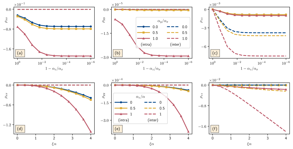
Figure 3: The intraband (solid lines) and interband (dashed lines) contributions to the summation term in the superfluid-density tensor $\rho_{ij}$ are shown when $T=0$ and $U=U_{\uparrow\uparrow}=U_{\downarrow\downarrow}=10U_{\uparrow\downarrow}/9.$ Here the left, middle and right columns correspond, respectively, to the diagonal elements $\rho_{xx}$, $\rho_{yy}$ and $\rho_{zz}$ (in units of $n_{0}\approx n$), and all of the off-diagonal elements vanish. In the top panel the diagonal elements are shown as a function of $\alpha_{z}$ for three values of $\alpha_{y}$ when $\alpha_{x}=2/\xi$ is fixed. In the bottom panel the diagonal elements are shown as a function of the SOC strength $\alpha=\alpha_{x}=\alpha_{y}$ for three values of the $\alpha_{z}/\alpha$ ratio.

Since we are interested only in the low-$\mathbf{Q}$ limit of $\Omega_{\mathbf{Q}}$, we can use the Taylor expansion $\ln\det\mathbf{G}_{\mathbf{Q}\ell\mathbf{q}}^{-1}=\mathrm{Tr}\ln\mathbf{G}_{\mathbf{0}\ell\mathbf{q}}^{-1}-\mathrm{Tr}\sum_{l=1}^{\infty}(\mathbf{G}_{\mathbf{0}\ell\mathbf{q}}\mathbf{\Sigma}_{\mathbf{Q}})^{l}/l,$ and keep up to second-order terms in $\mathbf{\Sigma}_{\mathbf{Q}}$. This calculation leads to

$$\rho_{ij}= mn_{0}M^{-1}_{ij}-\frac{mT}{2V}\sum_{\ell\mathbf{q}}^{\prime}\big{[}\mathrm{Tr}\big{(}\mathbf{G}_{\mathbf{0}\ell\mathbf{q}}\partial_{i}\partial_{j}\mathbf{H}_{\mathbf{q}}\big{)}$$

$$+\mathrm{Tr}\big{(}\mathbf{G}_{\mathbf{0}\ell\mathbf{q}}\tau_{z}\partial_{i}\mathbf{H}_{\mathbf{q}}\mathbf{G}_{\mathbf{0}\ell\mathbf{q}}\tau_{z}\partial_{j}\mathbf{H}_{\mathbf{q}}\big{)}\big{]}.$$ (25)

Here the first term is due to the kinetic energy of the condensate in the presence of an SF flow, i.e., there is an additional quadratic contribution $(N_{0}/2)\sum_{ij}Q_{i}Q_{j}M^{-1}_{ij}$ to $\Omega_{zp}$ coming from the low-$\mathbf{Q}$ expansion of $\sum_{\mathbf{k}}\xi_{-,\mathbf{k+Q}}a_{-,\mathbf{k}}^{\dagger}a_{-,\mathbf{k}}$ around $\mathbf{k_{0}}$. Thus, when the inverse of the effective-mass tensor $M^{-1}_{ij}$ vanishes, $\rho_{ij}$ is determined entirely by the Bogoliubov Hamiltonian, i.e., the quantum fluctuations above the condensate. The trace of the Green’s function in the second term is related to the density of excited (non-condensate) particles $n_{e}$ since its diagonal elements yield $n_{e}=-(T/V)\sum_{\ell\mathbf{q}}^{\prime}\big{(}G_{\mathbf{0}\ell\mathbf{q}}^{11}+G_{\mathbf{0}\ell\mathbf{q}}^{22}\big{)}e^{-i\omega_{\ell}0^{+}},$ or alternatively, $n_{e}=-(T/V)\sum_{\ell\mathbf{q}}^{\prime}\big{(}G_{\mathbf{0}\ell\mathbf{q}}^{33}+G_{\mathbf{0}\ell\mathbf{q}}^{44}\big{)}e^{i\omega_{\ell}0^{+}}.$ Thus, by performing the summation over the Matsubara frequencies, we eventually obtain

$$\rho_{ij}=n_{t}\delta_{ij}-n_{0}\frac{\alpha_{y}^{2}\delta_{iy}+\alpha_{z}^{2}\delta_{iz}}{\alpha_{x}^{2}}+\frac{m}{2V}\sum_{nn^{\prime}ss^{\prime}\mathbf{q}}^{\prime}ss^{\prime}\langle\chi_{s\mathbf{q}}^{n}|\tau_{z}$$

$$\partial_{i}\mathbf{H}_{\mathbf{q}}|\chi_{s^{\prime}\mathbf{q}}^{n^{\prime}}\rangle\langle\chi_{s^{\prime}\mathbf{q}}^{n^{\prime}}|\tau_{z}\partial_{j}\mathbf{H}_{\mathbf{q}}|\chi_{s\mathbf{q}}^{n}\rangle\frac{f_{\mathrm{B}}(E_{s\mathbf{q}}^{n})-f_{\mathrm{B}}(E_{s^{\prime}\mathbf{q}}^{n^{\prime}})}{E_{s\mathbf{q}}^{n}-E_{s^{\prime}\mathbf{q}}^{n^{\prime}}},$$ (26)

where $n_{t}=n_{0}+n_{e}$ is the total density of particles in the system and $f_{\mathrm{B}}(x)$ is the Bose-Einstein distribution function. Here a partial derivative $\partial f_{\mathrm{B}}(E_{s\mathbf{q}}^{n})/\partial E_{s\mathbf{q}}^{n}=-[1/(4T)]\mathrm{cosech}^{2}\left[E_{s\mathbf{q}}^{n}/(2T)\right]$ is implied when the summation indices coincide simultaneously ($n=n^{\prime}$ and $s=s^{\prime}$). In comparison to the SF density, the non-condensate density can be written as

$$n_{\mathrm{e}} =\frac{1}{2V}\sum_{ns\mathbf{q}}^{\prime}s\big{[}\langle\chi_{s\mathbf{q}}^{n}|\chi_{s\mathbf{q}}^{n}\rangle f_{\mathrm{B}}(E_{s\mathbf{q}}^{n})+{{}_{2}\langle}\chi_{s\mathbf{q}}^{n}|\chi_{s\mathbf{q}}^{n}\rangle_{2}\big{]},$$ (27)

$$=\frac{1}{2V}\sum_{ns\mathbf{q}}^{\prime}\big{[}s\langle\chi_{s\mathbf{q}}^{n}|\chi_{s\mathbf{q}}^{n}\rangle f_{\mathrm{B}}(E_{s\mathbf{q}}^{n})-1/2\big{]}.$$ (28)

We checked that both expressions yield the same numerical result. Note that $n_{\mathrm{e}}^{0}=[1/(2V)]\sum_{n\mathbf{q}}^{\prime}(-1+\langle\chi_{-,\mathbf{q}}^{n}|\chi_{-,\mathbf{q}}^{n}\rangle)$ is the so-called quantum depletion of the condensate at $T=0$.

As an illustration, in the case of a single-component Bose gas, there is a single Bogoliubov band with the usual quasiparticle-quasihole symmetric spectrum $E_{s\mathbf{q}}=sE_{\mathbf{q}}$ where $E_{\mathbf{q}}=\sqrt{\varepsilon_{\mathbf{q}}(\varepsilon_{\mathbf{q}}+2Un_{0})},$ and by plugging $\langle\chi_{s\mathbf{q}}|\tau_{z}\partial_{i}\mathbf{H}_{\mathbf{q}}|\chi_{s^{\prime}\mathbf{q}}\rangle=(sq_{i}/m)\delta_{ss^{\prime}}$ into Eq. (26), we recover the textbook definition $\rho_{ij}=n_{t}\delta_{ij}+[1/(mV)]\sum_{\mathbf{q}}^{\prime}q_{i}q_{j}\partial f_{\mathrm{B}}(E_{\mathbf{q}})/\partial E_{\mathbf{q}}$ of $\rho_{s}$ fetter . This shows that $\rho_{ij}=n_{t}\delta_{ij}$ at zero temperature and that the entire gas is SF. Similarly, by plugging $\langle\chi_{s\mathbf{q}}|\chi_{s^{\prime}\mathbf{q}}\rangle=(\varepsilon_{\mathbf{q}}+Un_{0})/E_{\mathbf{q}}$ into Eq. (28), we recover the textbook definition of $n_{e}=n_{e}^{0}+n_{e}^{T}$, where $n_{e}^{0}=[1/(2V)]\sum_{\mathbf{q}}^{\prime}[-1+(\varepsilon_{\mathbf{q}}+Un_{0})/E_{\mathbf{q}}]$ is the quantum depletion and $n_{e}^{T}=(1/V)\sum_{\mathbf{q}}^{\prime}(\varepsilon_{\mathbf{q}}+Un_{0})f_{\mathrm{B}}(E_{\mathbf{q}})/E_{\mathbf{q}}$ is the thermal one fetter .

We note in passing that Eq. (26) is consistent with the so-called SF weight that is derived in Ref. julku21a ; julku21b for a multi-band Bloch Hamiltonian. See also yangnote . Unlike our phase-twist method, they define the SF weight as the long-wavelength and zero-frequency limit of the current-current linear response. In particular our expression for a continuum model is formally equivalent to their $D_{1,\mu\nu}^{s}+D_{2,\mu\nu}^{s}+D_{3,\mu\nu}^{s}$ with the caveat that $D_{2,\mu\nu}^{s}$ is cancelled by the interband contribution of $D_{1,\mu\nu}^{s}$. This is similar to the cancellation that they observed for the Kagome lattice. Furthermore Eq. (26) can also be split into two parts $\rho_{ij}=\rho_{ij}^{\mathrm{intra}}+\rho_{ij}^{\mathrm{inter}}$ depending on the physical origin of the terms julku21a ; julku21b : the intraband (interband) processes give rise to the conventional (geometric) contribution. This division is motivated by the success of a similar description with Fermi SFs iskin18a ; julku18 .

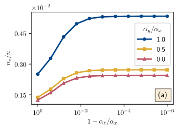
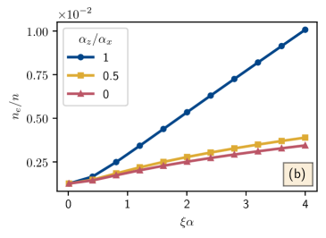
Figure 4: Quantum depletion of the condensate density is shown as a function of SOC parameters when $T=0$ and $U=U_{\uparrow\uparrow}=U_{\downarrow\downarrow}=10U_{\uparrow\downarrow}/9.$ The fraction of the depletion is plotted (a) as a function of $\alpha_{z}$ for three values of $\alpha_{y}$ when $\alpha_{x}=2/\xi$ is fixed, and (b) as a function of the SOC strength $\alpha=\alpha_{x}=\alpha_{y}$ for three values of the $\alpha_{z}/\alpha$ ratio.

In order to provide further evidence for its geometric origin, in Fig. 3 we compare the interband contribution with that of the intraband one coming from the summation term in Eq. (26). Here we set $T\to 0$. First of all this figure shows that the total contribution from the summation term decreases with the increased strength and isotropy of the SOC fields, i.e., when $\alpha_{y}\to\alpha_{x}$ in Figs. 3(a,b,c) and when $\alpha_{z}\to\alpha$ in Figs. 4(d,e,f). Thus $\rho_{xx}$ always decreases from $n_{t}$ with SOC. However, depending on the value of $\alpha_{y}$ and $\alpha_{z}$, the remaining contribution $n_{e}+n_{0}(\alpha_{x}^{2}-\alpha_{y}^{2}\delta_{iy}-\alpha_{z}^{2}\delta_{iz})/\alpha_{x}^{2}$ to $\rho_{yy}$ and $\rho_{zz}$ in Eq. (26) may compete with or favor the contribution from the summation term. More importantly Fig. 3 shows that not only $\rho_{zz}$ has the largest interband contribution but also its relative weight is predominantly controlled by $\alpha_{z}\neq 0$. These findings are in support of our Bogoliubov dispersion given in Eq. (20) whose quantum-geometric contributions are fully controlled by $\alpha_{z}\neq 0$. For completeness, in Fig. 4 we present the quantum depletion $n_{e}^{0}$ as a function of SOC parameters when $U=U_{\uparrow\uparrow}=U_{\downarrow\downarrow}=10U_{\uparrow\downarrow}/9.$ This figure shows that $n_{e}^{0}$ increases with the increased strength and isotropy of the SOC fields cui13 , i.e., when $\alpha_{y}\to\alpha_{x}$ in Fig. 4(a) and when $\alpha_{z}\to\alpha$ in Fig. 4(b). This is clearly a direct consequence of the increased degeneracy of the single-particle spectrum. However, since $n_{e}^{0}\ll n$ even for moderately strong SOC fields, the Bogoliubov approximation is expected to work well in general.

V Conclusion

To summarize here we considered the plane-wave BEC phase of a spin-orbit-coupled Bose gas and reexamined its SF properties from a quantum-geometric perspective. In order to achieve this task analytically, we first reduce the $4\times 4$ Bogoliubov Hamiltonian (that involves both lower and upper helicity bands) down to $2\times 2$ through projecting the system onto the lower helicity band. This is motivated by the assumption that the energy gap between the lower and upper helicity bands nearby the single-particle ground state is much larger than the interaction energy. Then, given our numerical verification that the projected Hamiltonian provides an almost perfect description for the lower (higher) quasiparticle (quasihole) branch in the Bogoliubov spectrum, we exploited the low-momentum Bogoliubov spectrum analytically and identified the geometric contributions to the sound velocity. In contrast to the conventional contribution that has a square-root dependence on the interaction strength, we found that the geometric ones are distinguished by a linear dependence. It may be important to emphasize that these geometric effects are not caused by the negligence of the upper helicity band. Similar to the Fermion problem where the geometric effects dress the effective mass of the Goldstone modes iskin20a ; iskin20b , here one can also interpret the geometric terms in terms of a dressed effective mass for the Bogoliubov modes. We also discussed the roton instability of the plane-wave ground state against the stripe phase and determined the phase transition boundary. In addition we derived the SF density tensor by imposing a phase-twist on the condensate order parameter and analyzed the relative importance of its contribution from the interband processes that is related to the quantum geometry. As an outlook we believe it is worthwhile to do a similar analysis for the stripe phase.

- (1) S. Peotta and P. Törmä, Superfluidity in topologically nontrivial flat bands, Nat. Commun. 6, 8944 (2015).
- (2) L. Liang, T. I. Vanhala, S. Peotta, T. Siro, A. Harju, and P. Törmä, Band geometry, Berry curvature, and superfluid weight, Phys. Rev. B 95, 024515 (2017).
- (3) M. Iskin, Exposing the quantum geometry of spin-orbit-coupled Fermi superfluids, Phys. Rev. A 97, 063625 (2018).
- (4) M. Iskin, Quantum metric contribution to the pair mass in spin-orbit-coupled Fermi superfluids, Phys. Rev. A 97, 033625 (2018).
- (5) M. Iskin, Geometric contribution to the Goldstone mode in spin-orbit-coupled Fermi superfluids, Physica B 592, 412260 (2020).
- (6) M. Iskin, Collective excitations of a BCS superfluid in the presence of two sublattices, Phys. Rev. A 101, 053631 (2020).
- (7) A. Julku, L. Liang, and P. Törmä, Superfluid weight and Berezinskii-Kosterlitz-Thouless temperature of spin-imbalanced and spin-orbit-coupled Fulde-Ferrell phases in lattice systems, New J. Phys. 20, 085004 (2018).
- (8) Z. Wang, G. Chaudhary, Q. Chen, and K. Levin, Quantum geometric contributions to the BKT transition: Beyond mean field theory, Phys. Rev. B 102, 184504 (2020).
- (9) P. Törmä, L. Liang, and S. Peotta, Quantum metric and effective mass of a two-body bound state in a flat band, Phys. Rev. B 98, 220511(R) (2018).
- (10) M. Iskin, Two-body problem in a multiband lattice and the role of quantum geometry, Phys. Rev. A 103, 053311 (2021). See also arXiv:2109.06000.
- (11) A. Julku, G. M. Bruun, and P. Törmä, Quantum Geometry and Flat Band Bose-Einstein Condensation, Phys. Rev. Lett. 127, 170404 (2021).
- (12) A. Julku, G. M. Bruun, and P. Törmä, Excitations of a Bose-Einstein condensate and the quantum geometry of a flat band, Phys. Rev. B 104, 144507 (2021).
- (13) Towards the completion of this work, we became aware of an independent study yang21 , where the SF density tensor is derived for a two-dimensional system using the linear-response theory. The results seem to agree with ours when there is an overlap.
- (14) L. Yang, Quantum-fluctuation-induced superfluid density in two-dimensional spin-orbit-coupled Bose-Einstein condensates, Phys. Rev. A 104, 023320 (2021).
- (15) Y. Li, G. I. Martone, S. Stringari, Bose-Einstein condensation with spin-orbit coupling, Annu. Rev. Cold At. Mol. 3, 201 (2015).
- (16) H. Zhai, Degenerate quantum gases with spin-orbit coupling: a review, Rep. Prog. Phys. 78, 026001 (2015).
- (17) Y. Zhang, M. E. Mossman, T. Busch, P. Engels, and C. Zhang, Properties of spin-orbit-coupled Bose-Einstein condensates, Front. Phys. 11(3), 118103 (2016).
- (18) X. Cui and Q. Zhou, Enhancement of condensate depletion due to spin-orbit coupling, Phys. Rev. A 87, 031604(R) (2013).
- (19) T. Ozawa and G. Baym, Stability of Ultracold Atomic Bose Condensates with Rashba Spin-Orbit Coupling against Quantum and Thermal Fluctuations, Phys. Rev. Lett. 109, 025301 (2012).
- (20) G. Baym and T. Ozawa, Condensation of bosons with Rashba-Dresselhaus spin-orbit coupling, J. Phys.: Conf. Ser. 529, 012006 (2014).
- (21) C. Wang, C. Gao, C.-M. Jian, and Hui Zhai, Spin-Orbit Coupled Spinor Bose-Einstein Condensates, Phys. Rev. Lett. 105, 160403 (2010).
- (22) R. Barnett, S. Powell, T. Graß, M. Lewenstein, and S. Das Sarma, Order by disorder in spin-orbit-coupled Bose-Einstein condensates, Phys. Rev. A 85, 023615 (2012).
- (23) L. Santos, G. V. Shlyapnikov, and M. Lewenstein, Roton-Maxon Spectrum and Stability of Trapped Dipolar Bose-Einstein Condensates, Phys. Rev. Lett. 90, 250403 (2003).
- (24) S. Saccani, S. Moroni, and M. Boninsegni, Excitation Spectrum of a Supersolid, Phys. Rev. Lett. 108, 175301 (2012).
- (25) T. Macrì, F. Maucher, F. Cinti, and T. Pohl, Elementary excitations of ultracold soft-core bosons across the superfluid-supersolid phase transition, Phys. Rev. A. 87, 061602 (2013).
- (26) J.-N. Schmidt, J. Hertkorn, M. Guo, F. Böttcher, M. Schmidt, K. S. H. Ng, S. D. Graham, T. Langen, M. Zwierlein, and T. Pfau, Roton Excitations in an Oblate Dipolar Quantum Gas, Phys. Rev. Lett. 126, 193002 (2021).
- (27) F. Böttcher, J.-N. Schmidt, J. Hertkorn, K. S. H. Ng, S. D. Graham, M. Guo, T. Langen, and T. Pfau, New states of matter with fine-tuned interactions: quantum droplets and dipolar supersolids, Rep. Prog. Phys. 84, 012403 (2021).
- (28) M. A. Khamehchi, Y. Zhang, C. Hamner, T. Busch, and P. Engels, Measurement of collective excitations in a spin-orbit-coupled Bose-Einstein condensate, Phys. Rev. A. 90, 063624 (2014).
- (29) S.-C. Ji, L. Zhang, X.-T. Xu, Z. Wu, Y. Deng, S. Chen, and J.-W. Pan, Softening of Roton and Phonon Modes in a Bose-Einstein Condensate with Spin-Orbit Coupling, Phys. Rev. Lett. 114, 105301 (2015).
- (30) J.-R. Li, J. Lee, W. Huang, S. Burchesky, B. Shteynas, F. C. Top, A. O. Jamison, and W. Ketterle, A stripe phase with supersolid properties in spin-orbit-coupled Bose-Einstein condensates, Nature 543, 91 (2017).
- (31) A. Putra, F. S.-Cárcoba, Y. Yue, S. Sugawa, and I. B. Spielman, Spatial Coherence of Spin-Orbit-Coupled Bose Gases, Phys. Rev. Lett. 124, 053605 (2020).
- (32) Y. Li, G. I. Martone, L. P. Pitaevskii, and S. Stringari, Superstripes and the Excitation Spectrum of a Spin-Orbit-Coupled Bose-Einstein Condensate, Phys. Rev. Lett. 110, 235302 (2013). See also the more recent analysis by G. I. Martone and S. Stringari, Supersolid phase of a spin-orbit-coupled Bose-Einstein condensate: a perturbation approach, submitted to SciPost (2021).
- (33) Y.-C. Zhang, Z.-Q. Yu, T. K. Ng, S. Zhang, L. Pitaevskii, and S. Stringari, Superfluid density of a spin-orbit-coupled Bose gas, Phys. Rev. A 94, 033635 (2016)
- (34) X.-L. Chen, J. Wang, Y. Li, X.-J. Liu, and H. Hu, Quantum depletion and superfluid density of a supersolid in Raman spin-orbit-coupled Bose gases, Phys. Rev. A 98, 013614 (2018).
- (35) E. Taylor, A. Griffin, N. Fukushima, and Y. Ohashi, Pairing fluctuations and the superfluid density through the BCS-BEC crossover, Phys. Rev. A 74, 063626 (2006).
- (36) L. He and X.-G. Huang, BCS-BEC crossover in three-dimensional Fermi gases with spherical spin-orbit coupling, Phys. Rev. B 86, 014511 (2012).
- (37) A. L. Fetter and J. D. Walecka, Quantum Theory of Many-Particle Systems (McGraw-Hill, 1971).