Berezinskii–Kosterlitz–Thouless transition – a universal neural network study with benchmarking

Abstract

Using a supervised neural network (NN) trained once on a one-dimensional lattice of 200 sites, we calculate the Berezinskii–Kosterlitz–Thouless phase transitions of the two-dimensional (2D) classical $XY$ and the 2D generalized classical $XY$ models. In particular, both the bulk quantities Binder ratios and the spin states of the studied systems are employed to construct the needed configurations for the NN prediction. By applying semiempirical finite-size scaling to the relevant data, the critical points obtained by the NN approach agree well with the known results established in the literature. This implies that for each of the considered models, the determination of its various phases requires only a little information. The outcomes presented here demonstrate convincingly that the employed universal NN is not only valid for the symmetry breaking related phase transitions, but also works for calculating the critical points of the phase transitions associated with topology. The efficiency of the used NN in the computation is examined by carrying out several detailed benchmark calculations.

I Introduction

Recently, techniques of Machine Learning (ML), such as supervised neural network (NN), autoencoder, as well as generative adversarial network (GAN) provide alternative approaches for studying many-body physics. In particular, these ML methods are shown to be efficient in classifying various phases of physical systems Wan16 ; Oht16 ; Car16 ; Tro16 ; Chn16 ; Tan16 ; Nie16 ; Den17 ; Zha17 ; Hu17 ; Li18 ; Zha18 ; Bea18 ; Lia19 ; Rod19 ; Car19 ; Zha19 ; Don19 ; Tan20.1 ; Tan20.2 ; Sin20 ; Sch20 ; Carrasquilla:2020mas ; Tomita:2020ylz . They are employed in the studies of high energy physics and astronomy as well Baldi:2014pta ; Hoyle:2015yha ; Mott:2017xdb ; Pang:2016vdc ; Sha18 ; Cavaglia:2018xjq ; Larkoski:2017jix ; Amacker:2020bmn ; Aad:2020cws ; Cabero:2020eik ; Nicoli:2020njz . To conclude, ML has gone far beyond its original fields of applications such as computer, information, and medical sciences.

The employment of NN in studying many-body systems usually consists of three stages, namely the training, the validation, and the testing (prediction) stages Car19 ; Carrasquilla:2020mas . Here we will briefly describe the stages of training and testing. The standard training set typically used in a NN calculation associated with investigating phase transition consists of several to a few thousand real configurations Car16 . As a result, the calculations are quite demanding. Apart from this, the NNs commonly employed have complicated infrastructure such as the convolutional neural network (CNN). Moreover, for any given model, special structure of the convolutional layer is designed for that model Car19 ; Carrasquilla:2020mas . The idea of using CNN is to capture the features of the system so that the NN can efficiently learn to distinguish various phases. From this point of view, a CNN built for a model may not be applicable for another system. Besides, for every studied model and each of the considered system sizes, a separate training is required. Finally, for the testing stage, real configurations are employed for the prediction. This would use huge amount of storage space if system of larger sizes are considered. Although the ideas from NN are shown to be able to study the critical phenomena of phase transitions, the facts that a training should be conducted whenever a new model or a different system size is considered, as well as the need of large storage space may prevent NN from being practically used in real investigations.

Because of these potential hindrances, it is desirable to construct a NN that can be used to study various phases of many models, and during the same time is efficient in both the computation and the storage. It is also interesting to notice that the majority of the studies associated with using the NN method to investigate phase transitions have focused on modifying the infrastructure of the NNs, and seldom provide benchmarks of the performance of the used NNs.

In Ref. Tan21 , a simple NN trained on a one-dimensional (1D) lattice using only two configurations as the training set is built (using Keras and Tensorflow kera ; tens ). The obtained (only one) NN successfully calculates the critical points of several three-dimensional models. In particular, both the (spin) configurations and the bulk observables are employed to construct the needed configurations, which are 1D lattices of 120 sites, for the NN prediction. Since only 1D configurations are required, the storage needed for the prediction stage is only at the permille level of that necessary for a standard NN calculation. An estimated benchmark also indicates the 1D NN is extremely efficient in the training stage Tan21 . Particularly, for the 3D classical $O(3)$ model, the time needed to train a NN using the standard approach with total 1000 configurations obtained at 4 temperatures and system size $L=48$ is at least 400 times as much as that required for the 1D NN. It should also be pointed out that the 1D NN of Ref. Tan21 is one of the few supervised NN approaches for studying phase transitions that the locations of the critical points (in the associated parameter spaces) are not required in advance.

The phase transitions corresponding to the models considered in Ref. Tan21 are induced by symmetry breaking and restoration. Hence it will be interesting to examine whether the constructed 1D NN is applicable to locate the critical point(s) associated with topological phase transitions. We would like to emphasize the fact that the majority of NN studies related to topological phase transitions use techniques of unsupervised NN instead of supervised NN. Consequently, it is motivated to conduct a supervised NN investigation for a topological phase transition, and particularly to examine whether the obtained outcomes are comparable in precision with those determined by unsupervised NN methods. Because of the reasons mentioned above, here we have used the 1D NN built in Ref. Tan21 to study the phase transitions of the two-dimensional (2D) classical $XY$ and the 2D generalized classical $XY$ models.

To calculate the critical point associated with the Berezinskii–Kosterlitz–Thouless (BKT) phase transition of the 2D classical $XY$ model, the standard approach is to determine the helicity modulus at finite lattices, and then applies the expected finite-size scaling (Which contains a logarithmic correction) to obtain the bulk critical point. Other quantities such as Binder ratios are seldom considered for such investigations. In this study observables which satisfy certain conditions (detailed later) will be used. In particular, the Binder ratios will be considered in the NN calculations.

Remarkably, using the 1D NN as well as the configurations constructed from the Binder ratios (and the spins), the critical points calculated by applying semiempirical finite-size scaling to the obtained relevant quantities are in good agreement with the known results in the literature. Our investigations indicate that in addition to the helicity modulus, the observables Binder ratios in conjunction with the NN techniques provides an efficient alternative approach for studying the phase transitions of BKT type. Although BKT type transitions are typically characterized by vortices, as we will show later, our outcomes imply that even few percent information of the whole spin configurations can be employed to detect the existence of a BKT transition.

The results presented here demonstrate that the used 1D NN is valid for both symmetry breaking and topology related phase transitions. In other words, the employed 1D NN is universal from a broaden point of view.

It is beyond doubt that the storage space needed for the prediction in this study is much less than the methods of using real configurations for the prediction. Apart from this, we also conduct some benchmark calculations to examine the efficient of our methods in both the training and the prediction stages. The results imply potentially a factor of at least several hundred to few thousand in efficiency is gained for our methods.

II The constructed supervised Neural Network

It should be pointed out that we hope to construct a supervised NN that is applicable to as many models as possible when the phase transitions are concerned. During the same time, the efficiency in both the computation and the storage space should not be sacrificed. Based on such thoughts, in Ref. Tan21 a NN trained on a 1D lattice of a given fixed size is built. Moreover, it is shown as well that such a NN can be employed to determine the critical points of several 3D systems successfully. Therefore, in this study, the 1D NN of Tan21 is recycled and is adopted here. In other words, no NN, except those for the benchmarking calculations, is trained in this investigation.

To make current paper self-contained, some technical details including the constructed 1D NN are briefly quoted from Ref. Tan21 . The 1D NN employed here is a multilayer perceptron (MLP) which consists of only one input layer, one hidden layer of 512 independent nodes, and one output layer. Moreover, the algorithm considered for the whole NN steps is the minibatch. The adam and the categorical cross entropy are the optimizer and the loss function used. $L_{2}$ regularization is applied so that the overfitting can be prevented. The activation functions considered between various layers are the ReLU and the softmax functions. The details of the constructed MLP are shown in Fig. 1. Notice Fig. 1 indicates that the techniques of one-hot encoding and flatten are also included in the infrastructure of the used NN. Refs. Tan20.1 ; Tan20.2 ; Tan21 contain more detailed descriptions of the employed NN .

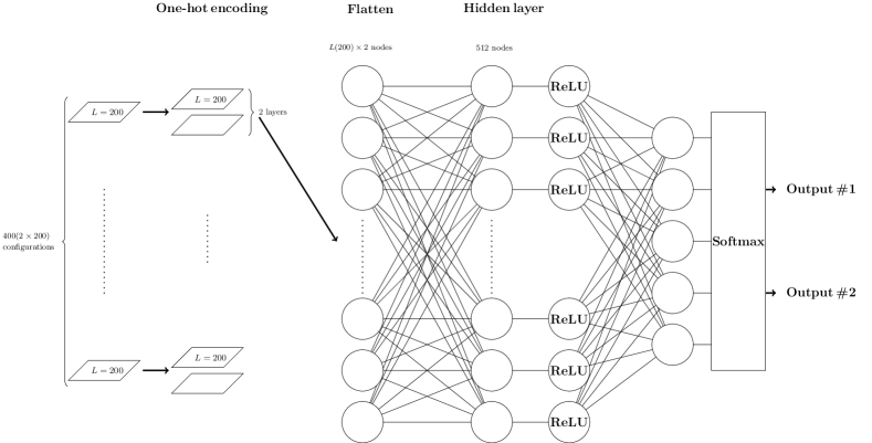
Figure 1: The NN (MLP), which consists of one input layer, one hidden layer, and one output layer, used here and in Refs. Tan20.1 ; Tan20.2 ; Tan21 . The training set are made up of 200 copies of only two configurations. There are 512 nodes in the hidden layer and each of these nodes is independently connected to every object in the training set. The steps of one-hot encoding and flatten are applied as well. The activation functions ReLU and softmax are employed in the associated layers. Finally, the output layer consists of two-component vector(s). The figure is reproduced from Refs. Tan20.1 ; Tan20.2 ; Tan21

For completeness, the training and the prediction strategies used in Ref. Tan21 will be introduced (quoted) for the benefit of readers. For the training set, instead of using real configurations obtained from the simulations, two artificial made configurations are employed. Particularly, one of the configuration has 0 as the value for each of its site, and every spot of the other configuration takes the number of 1. Because of the features of the considered training set, the corresponding labels are $(1,0)$ and $(0,1)$.

We would like to emphasize the fact that the employed NN was trained on a 1D lattice of 200 sites. Hence the training process takes much less computing resources than (any) other known schemes in the literature. We will provide some benchmarks later to demonstrate this fact. The considered approach for the NN prediction will be detailed later as well in the relevant sections.

It should be pointed out that 10 sets of random seeds are used so that there will be 10 MLPs. Each MLP will lead to an outcome which is the average over few hundred to several thousand results. The (final) main results quoted here are based on the means and the mean errors of the 10 outcomes. In other words, the errors shown here are associated with the NN, not the raw data.

III The microscopic models and observables

The Hamiltonian $H$ of the studied 2D generalized classical $XY$model on the square lattice is given by Has05 ; Can14 ; Can16

$$H=-\sum_{\left<ij\right>}\Delta\cos\left(\theta_{i}-\theta_{j}\right)-\left(1-\Delta\right)\cos\left(q\theta_{i}-q\theta_{j}\right),$$ (1)

where the summation is over nearest neighbor $i$ and $j$, $q$ is some (positive) integer, and $0\leq\theta_{i}\leq 2\pi$. When $\Delta=1$, the above Hamiltonian reduces to that of the standard 2D classical $XY$ model. In our study, we will consider the case of $\Delta=0.25$ and $q=3$.

Relevant observables used in this study are the first and the second Binder ratios which are given as

$$Q_{1,j}=\langle|m_{j}|\rangle^{2}/\langle m_{j}^{2}\rangle\,\,\text{and}\,\,Q_{2,j}=\langle m_{j}^{2}\rangle^{2}/\langle m_{j}^{4}\rangle,$$ (2)

respectively. Here $j=1$ or (and) 3, $m_{j}=\frac{1}{L^{2}}\sum_{k}\exp\left(i\theta_{k}j\right)$ and $L$ is the linear box size of the system Bin81 . Unless confusion may arise, the subscript $j$ in $Q_{1,j}$ and $Q_{2,j}$ will be omitted.

IV Benchmarks of the performance of the employed 1D NN

Before presenting the numerical results, we would like to show some benchmarks of the performance of the employed 1D NN here. The considered model for the benchmark investigation is the 2D classical XY model. We have carried out the associated calculations using both a CNN and a MLP. Comparison between the performance regarding the training of the employed 1D NN and a autoencoder is shown as well. The benchmark investigations are done on a server with 24 cores (two opteron 6344) and 96G memory. The installed version of tensorflow uses multiple CPUs for the calculations by default. Hence we keep only one training job running on the server at a time. It should be pointed out that the outcomes of the benchmarks may change due to some facts such as what machine is used for the calculations (CPU or GPU) and the jobs loading in that machine. Installing the tensorflow with different (versions of) libraries and how the executed codes are implemented would affect the benchmarks as well. Nevertheless, the benchmarking shown here provides useful information regarding the performance of the considered NNs. Finally, tunable parameters associated with NN not mentioned explicitly in the text are the default ones.

Unlike the main outcomes which will be demonstrated later, the shown mean errors in this section are associated with the raw data, i.e. we use one NN, not 10 NNs for the calculations.

IV.1 Benchmarks using a MLP

The employed MLP consists of one input layer, one hidden layer of 512 nodes, and one output layer. The epochs and the batch size used in the calculations are 800 and 40, respectively. Moreover, three calculations using various training strategies are conducted. The details are as follows.

1. For each of $L=64$, 96, and 128, 12 temperatures (6 below and 6 above the critical point) with each temperature having 1000 real configurations are considered. In addition, the variable $\theta_{i}$ at each site $i$ is converted to $\theta_{i}\,\text{mod}\,\pi$, and the resulting configurations are used as the training set. The step of one-hot encoding is employed as well.

2. For each of $L=64$, 96, and 128, 12 temperatures (6 below and 6 above the critical point) with each temperature having 1000 real configurations are used as the training set. The raw spin configurations are used directly as the training set and the step of one-hot encoding is not employed. Based on the relevant publications in the literature, this training procedure is the standard method of training the needed NN for studying the 2D classical $XY$ model.

3. 200 copies for each of the two artificial configurations described in the previous section are used as the training set. One-hot encoding is considered.

For convenience, These three investigations (from top to bottom) will be name the first, the second, and the third (training) methods. The total time takes to complete the whole training processes for each of the three different training strategies is as follows.

1. First training method: 2233.2 minutes (The time needed for training the $L=128$ data is 1227.3 minutes).

2. Second training method: 1078.4 minutes (The time needed for training the $L=128$ data is 605.27 minutes).

3. Third training method: 1.2 minutes.

The results indicate that the time required to train a MLP using the first method is about 2000 times as much as that needed to train a MLP with the third method. The time required for the prediction associated with the first training method is also several times as much as that needed for the prediction related to the third training approach.

The NN prediction using these three trained NN and the real spin configurations of $L=128$ leads to the outcomes demonstrated in Fig. 2. For the NN obtained using the third training method, each of the configurations employed for the prediction is built by firstly choosing 200 spins (randomly) from the raw $128^{2}$ spins, and then using the associated $\theta\,\text{mod}\,\pi$ to construct the needed 200 sites configuration (for the prediction).

The left and right panels of Fig. 2 are associated with the first and the third training methods, respectively. In addition, the intersecting points and the vertical dashed lines in these two panels are the NN predicted and the expected $\beta_{\text{KT}}$ for the 2D classical $XY$ model, respectively. The outcomes related to the second training method are not shown because the training is not successful. Indeed, for the second training approach, the simple MLP used for the training can hardly learn any information of the system from the raw spin configurations. Finally, the fact that the use of $\theta\,\text{mod}\,\pi$ instead of $\theta$ can lead to an outcome that a simply built NN is capable of detecting the BKT transition is quite remarkable.

It is beyond doubt that the results in Fig. 2 indicate the accuracy of the finite size critical $\beta$s obtained by the first and the third approaches are comparable with each other.

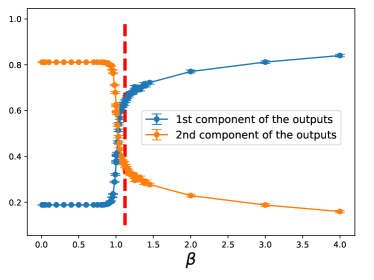
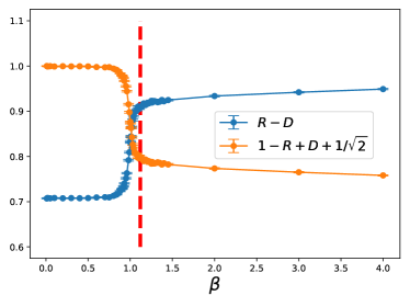
Figure 2: The MLP determination of the finite size critical inverse temperatures for the 2D classical $XY$ model (The system size is $L=128$). The left and the right panels correspond to the first and the third training methods, respectively, see the main text for the details. Here $R$ are the norms of the output vectors and $D$ is the difference between the $R$ of the smallest $\beta$ and $1/\sqrt{2}$.

IV.2 Benchmarks using a CNN

Ideally, the benchmark study should be conducted with a CNN that has been used in the literature. However, some details are typically missed in the relevant publications, for instance, the explicit expressions of the filters considered in Ref. Bea18 are not known. As a result, here we construct our own CNN for the investigations. The CNN considered here has one input layer, one convolutional layer, one average pooling layer, and one output layer.

For the CNN calculations, we use three training (and prediction) procedures as those associated with the MLP study described above. Notice the filter of the convolutional layer for the third training method is one-dimension, and the filters related to the second and the third training approaches are two-dimension. The resulting total time for each of the training strategies is as follows.

1. First training method: 580.9 minutes.

2. Second training method: 518.3 minutes.

3. Third training method: 1.0 minutes.

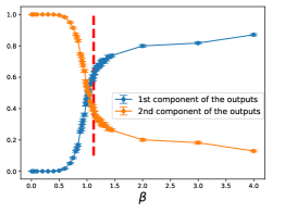
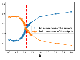
Figure 3: The CNN determination of the finite size critical inverse temperatures for the 2D classical $XY$ model (The system size is $L=128$). The left, the middle, and the right panels correspond to the first, the second, and the third training methods, respectively, see the main text for the details. Here $R$ are the norms of the output vectors and $D$ is the difference between the $R$ of the smallest $\beta$ and $1/\sqrt{2}$.

The results implies that the time required to train a CNN using either the first or the second methods is more than 500 times as much as that needed to train a CNN with the third method.

The CNN predictions are shown in Fig. 3. The left, the middle, and the right panels are the outcomes obtained from the CNNs trained by the first, the second, and the third method, respectively. The crossing points and the vertical lines in these panels are the CNN predicted and the expected critical points, respectively. Although the second method seems to lead to a result that is closest to $\beta_{\text{KT}}$, multiple crossing points are found for the left and the middle panels of Fig. 3. This will lead to large uncertainties for the estimated values of $\beta_{\text{KT}}$. One can build a more dedicated CNN, consider larger number of epochs, choose smaller learning rate, or use more data (close to $\beta_{\text{KT}}$) for the training so that the phenomenon of multiple crossing points does not show up. However, with these mended strategies the required training time could be (much) longer than that show above. It should also be pointed out that the crossing point depends on the chosen training set and the temperature interval (Which contains the true critical point) where the data associated with it are not included in the training set, see Fig. 4.

The determination of the crossing points associated with the third training method involves a factor $D$ which is the difference between the $R$ of the highest temperature and $1/\sqrt{2}$. As long as the $R$ of low temperatures saturate to a constant, the resulting crossing point should not depend on which highest temperature data is available (and used), see Fig. 5 which contains the crossings related to the highest temperature being 0.01 (left panel), 0.05 (middle panel), and 0.1 (right panel). Finally, although the crossing points in Fig. 5 seem to be less accurate than that related to the middle panel of Fig. 3, they are of high precision. This will lead to a better determination of the targeted quantity in finite-size scaling analysis.

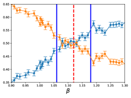
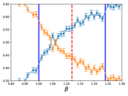
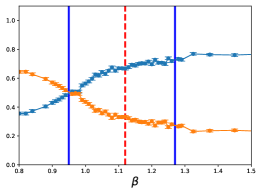
Figure 4: The CNN determination of the finite size critical inverse temperatures for the 2D classical $XY$ model using various training set (The system size is $L=128$). The trainings are conducted with the second method. In all panels, the vertical dashed lines are the expected $\beta_{\text{KT}}$, and the intervals bounded by the vertical solid lines are the regions where data associated with them are not used as the training set.

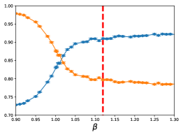
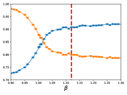
Figure 5: The CNN determination of the finite size critical inverse temperatures for the 2D classical $XY$ model (The system size is $L=128$). The results are associated with the third training method and are obtained using various $R$ corresponding to different highest temperatures, see the main text for the details.

IV.3 Comparison with a autoencoder

The first and the second training approaches shown above require the knowledge of the critical point in advance and this condition is less desirable since it is not always the case that the critical point is known for any given system. Hence the NN studies associated with topological phase transitions are usually conducted with unsupervised NNs. Here we also estimate the time requires to carry out the training for the autoencoder considered in Ref. Ale20 . Due to the infrastructure of the autoencoder built in Ref. Ale20 , the raw spin configurations cannot be employed directly, and we use the first method introduced above (but without considering the step of one-hot encoding) as the training strategy.

The total time needed for training the autoencoder is 1432.3 minutes, which is again more than 1000 times as much as that needed to train a MLP or a CNN with the third (training) method. In this study we do not conduct a detailed calculation of the prediction for the constructed autoencoder. A more systematic investigation will be presented in a future work.

IV.4 Remarks

One can construct a very dedicated and complicated CNN that has smooth data behavior with respect to $T$ ($\beta$) and is able to discover the BKT phase transition with high precision. This would then involve trial and error, and the obtained (complicated) CNN may only be valid for that studied system. Even for such a highly engineering CNN, one can still use the 2 artificial configurations introduced above as the training set, and it is anticipated that the associated comparisons of the efficiency in computation as well as the accuracy in prediction would be similar to those shown above.

V Numerical Results

In this section the results of applying the 1D NN to calculate the critical points of the considered models are presented. The associated Monte Carlo simulations are done using the Wolff algorithm Wol89 . We would like to emphasize the fact again that NO NEW NN IS TRAINED for obtaining the main results shown in this study. First of all, the outcomes associated with the 2D generalized classical $XY$ model are demonstrated.

V.1 Results associated with the 2D generalized classical $XY$ model

It is well known that for the 2D generalized classical $XY$ model studied here, two phase transitions will take place as one moves from the low temperature to the high temperature regions. Moreover, the first and the second phase transitions belong to the 3-state Potts (with critical temperature $T_{\text{Potts}}\sim 0.365$) and the BKT (with critical temperature $T_{\text{KT}}\sim 0.671$) universality classes, respectively Can14 ; Can16 .

V.1.1 Results using the spin configurations

To examine whether the employed 1D NN can detect these two phase transitions merely through (very small part of) the associated spin configurations, for each of the simulated temperatures and for every stored configuration with $L=128$, we have randomly chosen 200 sites ${j}$ and have used the $\theta_{j}\,\text{mod}\,\pi$ of these sites to construct a 200 sites 1D lattice to feed the NN. The magnitude $R$ of the resulting output vectors, obtained by this mentioned procedure, as a function of $T$ are shown in Fig. 6. It should be pointed out that in Fig. 6 the dashed and solid vertical lines represent the expected phase transitions related to the 3-state Potts and the BKT universality classes, respectively.

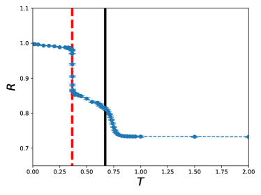
Figure 6: The magnitude $R$ of the outputs as a function of $T$ for the 2D generalized classical $XY$ model (The system size is $L=128$). The outcomes are obtained by using 200 spins ($\theta\,\text{mod}\,\pi$) randomly chosen from each of the real configurations. The vertical dashed and solid lines are the expected $T_{\text{Potts}}\sim 0.365$ and $T_{\text{KT}}\sim 0.671$, respectively.

Remarkably, as $T$ increases, the temperatures at which $R$ drops significantly are exactly located at those where the phase transitions occur. This strongly suggests that the used NN, which was trained on 1D lattice of 200 sites, is not only able to find phase transition associated with spontaneous symmetry breaking, but also can detect BKT type phase transition. It is remarkable as well that the results in Fig. 6 imply only (very) little information of the system is sufficient to detect change of states of that system.

As we will show later, if the Hamiltonian $H$ and the associated analytic investigation of $H$ are not known in advance, then the commonly use observables Binder ratios $Q_{i,1}$ can only detect the first phase transition (3-state Potts). Similarly, $Q_{i,3}$ or the helicity modulus can only find the 2nd transition of BKT type. With our simple NN, even with very LITTLE INFORMATION of the system one finds both the transitions. This can be considered as an advantage of NN approach over the traditional methods.

We would like to emphasize the fact that in Fig. 6, the drop of $R$ near $T_{\text{KT}}$ is slower than that close to $T_{\text{Potts}}$. This is consistent with the features of symmetry breaking and BKT type transitions since BKT type transition receives certain logarithmic corrections. It is remarkable that only few percent of the whole spin configurations can reveal the characteristics of the associated phase transitions.

To precisely calculate $T_{\text{Potts}}$ and $T_{\text{KT}}$, we have performed the same procedures for various system sizes. A preliminary investigation indicates $R\sim 1$ and $R\sim\sqrt{2/3}$ when $T\ll T_{\text{Potts}}$ and $T_{\text{Potts}}<T\leq T_{\text{KT}}$, respectively. In addition, $R$ $\sim$ $1/\sqrt{2}$ for $T\gg T_{\text{KT}}$. Using these results and the method introduced in Ref. Tan20.2 , the transition temperature $T_{\text{Potts,L}}$ corresponding to a given finite $L$ can be obtained by the intersection of $R$ and $1+\sqrt{2/3}-R$. Moreover, For a finite box size $L$ the related $T_{\text{KT,L}}$ is determined by the crossing point of $R-D$ and $\sqrt{2/3}+1/\sqrt{2}-R+D$, where $D$ is the difference between the $R$ of the (available) highest temperature and $1/\sqrt{2}$. The left and right panels of Fig. 7 demonstrate the critical temperatures obtained by this procedure for two system sizes $L=64$ and $L=128$.

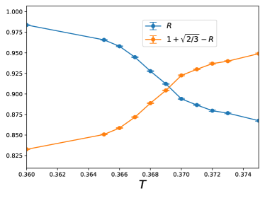
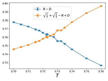
Figure 7: The determination of the finite size critical temperatures for the 2D generalized classical $XY$ model. The left and right panels correspond to box sizes $L=64$ (3-state Potts class) and $L=128$ (BKT), respectively. The outcomes are obtained by using 200 spins ($\theta\,\text{mod}\,\pi$) randomly chosen from each of the real configurations.

The intersecting points obtained by the above described strategies associated with the 3-state Potts and the BKT phase transitions are given as the left and the right panels of Fig. 8.

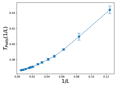
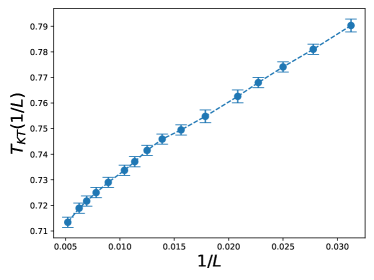
Figure 8: $T_{\text{Potts,L}}$ (left) and $T_{\text{KT,L}}$ (right) as functions of the system size $1/L$ for the 2D generalized classical $XY$ model. The outcomes are obtained by using 200 spins ($\theta\,\text{mod}\,\pi$) randomly chosen from each of the real configurations.

With a fit of the form $T_{\text{Potts,L}}=T_{\text{Potts}}+1/L^{\alpha}$ using all the data associated with the 3-state Potts class, one arrives at $T_{\text{Potts}}=0.3658(6)$ and $\alpha=1.52(9)$. The obtained $T_{\text{Potts}}=0.3658(6)$ agrees well with $T_{\text{Potts}}\sim 0.365$ determined in Refs. Can14 ; Can16 . Similarly, by fitting all the results related to the BKT transition with the ansatz $T_{\text{KT,L}}=T_{\text{K}}+b/(\log(L))^{2}+c/(\log(L))^{4}$ ($T_{\text{KT,L}}=T_{\text{K}}+b/(\log(L))^{2}$), one finds $T_{\text{KT}}=0.65(1)$ (0.657(3)) which is slightly below that calculated in Refs. Can14 ; Can16 (There $T_{\text{KT}}$ is found to be around 0.671). Considering the simplicity of the used NN as well as the difficulty in the calculations due to the logarithmic corrections associated with the BKT transition, the obtained $T_{\text{KT}}=0.65(1)$ is remarkably good.

V.1.2 Results using the Binder ratios

In addition to using raw spin configurations for the NN prediction, it is proposed and verified in Ref. Tan21 that bulk quantities that saturate to constants in the low and the high temperature regions can be employed to constructed the needed configurations for the NN prediction. Here we use this method to reinvestigate the BKT transition of the 2D generalized classical $XY$ model. Notice only several data points are needed to determine whether the targeted observable is appropriate for performing such calculations.

As can be seen in Fig. 9, the first Binder ratio $Q_{1,3}$ fulfills the condition of saturation very well. Consequently, $Q_{1,3}$ is perfectly suitable to carry out the associated calculations. It is interesting to notice that in Fig. 9 one sees that the magnitude of $Q_{1,3}$ remains a constant near $T_{\text{Potts}}$. In other words, $Q_{1,3}$ cannot be used to detect the phase transition associated with the 3-state Potts universality class. Similar situation occurs for $Q_{1,1}$. These observations in conjunction with Fig. 6 shown in the previous section strongly suggest that the NN approach has great potential to perform better than the traditional methods when phase transition is concerned.

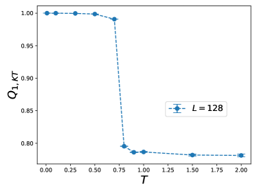
Figure 9: $Q_{1,3}$ (obtained on $128^{2}$ lattices) as a function of $T$ for the 2D generalized classical $XY$ model.

In our study, the Binder ratio $Q_{1,3}$ is used to construct the required configurations of 1D lattice with 200 sites for the prediction. For completeness, the detailed procedures are summarized as follows Tan21 . First, one performs the simulations with different $L$ and $T$. Second, for each simulated $L$, let $Q_{1,3}$ at the highest and the lowest temperatures be denoted by $Q_{\text{H}}$ and $Q_{\text{L}}$, respectively. In addition, $D_{L}$ is defined as $D_{L}=Q_{\text{L}}-Q_{\text{H}}$. With these notations, at every other temperature a configuration on a 1D lattice of 200 sites which will be used for the prediction is constructed through the following steps.

1. For a given temperature $T$, let the difference between the $Q_{1,3}$ at $T$ and $Q_{\text{H}}$ be $D_{T}$.

2. For each site $i$ of the 200 sites 1D lattice, choose a number $n$ in [0,1) randomly and uniformly.

3. If $n\geq|D_{T}/D_{L}|$, then the site $i$ is assigned the integer $1$. Otherwise the integer $0$ is given to $i$.

4. Repeat steps 1, 2 and 3 for all the simulated temperatures (or the inverse temperatures $\beta$).

The configurations constructed from steps 1 to 4 introduced above are fed to the trained NN. Then the associated critical point can be calculated by studying the temperature (or $\beta$) dependence of the output vectors $\vec{V}$. More specifically, if one treats $\vec{V}$ as functions of $T$ (or $\beta$), the critical point can be estimated to be at the temperature (or $\beta$) corresponding to the crossing point of the two curves built up from the components of $\vec{V}$. Apart from this, the critical point can be determined to be the temperature (or $\beta$) at which the output vector has the smallest value of magnitude as well.

We would like to point out that since with this method only bulk quantities satisfying certain conditions are needed for the NN prediction, the necessary storage space is much less than that for the standard approaches which require the whole spin states.

The intersections obtained through the steps introduced above are shown in Fig. 10. The employed bulk observable for reaching that figure is $Q_{1}$ and the system sizes $L$ for the left and the right panels of Fig. 10 are 48 and 96, respectively. In addition, the crossing points as a function of $1/L$ is demonstrated in Fig. 11.

By applying the finite-size scaling of the expression $T_{\text{KT,L}}=T_{\text{KT}}+b/(\log(L))^{2}+c/(\log(L))^{4}$ ($T_{\text{KT,L}}=T_{\text{KT}}+b/(\log(L))^{2}$) to all the data ($L\geq 96$ data) in Fig. 11, we arrive at $T_{\text{KT}}=0.674(5)$ ($T_{\text{KT}}=0.679(7)$) which is in excellent agreement with $T_{\text{KT}}\sim 0.671$ estimated in Refs. Can14 ; Can16 .

It is interesting to notice that the result calculated by using $Q_{1}$ seems more accurate than that obtained with part of the spin configurations. This may be due to the fact that $Q_{1}$ is a global quantity hence reveals more information of the system than that from part of the raw spin configurations.

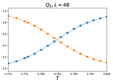
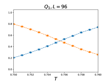
Figure 10: The intersecting points of the two components of the output vectors. The associated bulk quantity is $Q_{1}$. The left and the right panels are for the 2D generalized classical $XY$ model of system sizes $L=48$ and 96, respectively.

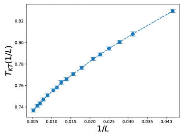
Figure 11: $T_{\text{KT}}$ (Which are obtained by the intersection method) as a function of the system size $1/L$ for the 2D generalized classical $XY$ model. The outcomes are obtained by the intersection method and are based on $Q_{1}$.

V.2 Results associated with the 2D classical $XY$ model

For the 2D classical $XY$ model, we will consider the approach of using the bulk observable(s) to determine the associated $T_{\text{KT}}$. Similar to the case of 2D generalized classical $XY$ model, the first and 2nd Binder ratios fulfill the saturation criterion, see Fig. 12. Therefore $Q_{1}$ will be employed for the calculations.

Fig. 13 shows the intersections of the two components of the output vectors. The left and the right panels are for $L=64$ and $L=128$, respectively.

The finite system inverse critical temperatures $\beta_{\text{KT,L}}$ of the 2D classical $XY$ model determined by the intersection idea is demonstrated in Fig. 14. Moreover, fits with the ansatz $\beta_{\text{KT,L}}=\beta_{\text{KT}}+b/(\log(L))^{2}+c/(\log(L))^{4}$ ($\beta_{\text{KT,L}}=\beta_{\text{KT}}+b/(\log(L))^{2}$) can lead to $\beta_{\text{KT}}=1.112(6)$ ($\beta_{\text{KT}}=1.107(7)$). The obtained values of $\beta_{\text{KT}}$ are in good agreement with $\beta_{\text{KT}}\sim 1.1199$ claimed in Ref. Has05 . During the analysis, we find that the values of $\beta_{\text{KT}}$ increase as fewer and fewer data of small $L$ are included in the fits. This indicates larger $L$ data may be needed in order to reach a high precision agreement.

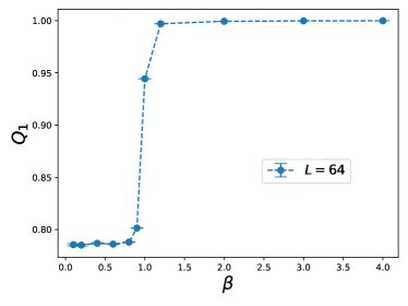
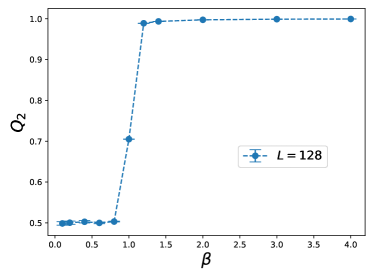
Figure 12: $Q_{1}$ (left panel, obtained on $64^{2}$ lattices) and $Q_{2}$ (right panel, obtained on $128^{2}$ lattices) as functions of $\beta$ for the 2D classical $XY$ model.

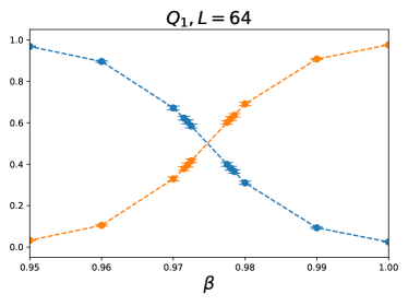
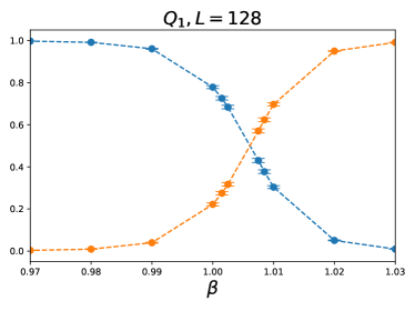
Figure 13: The intersecting points of the two components of the output vectors. The associated bulk quantity is $Q_{1}$. The left and the right panels are for the 2D classical $XY$ model of system sizes $L=64$ and $L=128$, respectively.

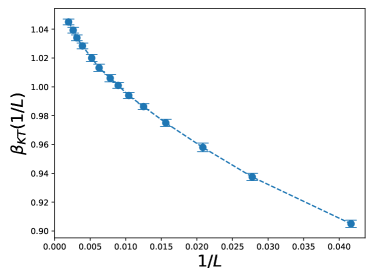
Figure 14: $\beta_{\text{KT}}$ as a function of the system size $1/L$ for the 2D classical $XY$ model. The outcomes are obtained by the intersection method and are based on $Q_{1}$.

VI Conclusions and Discussions

Using the NN constructed in Ref. Tan21 , which was trained on a 1D lattice of 200 sites, we calculate the critical points of the 2D classical $XY$ and the 2D generalized classical $XY$ models. We would like to stress again the following points.

1. In this study, no NN is trained. The employed NN is adopted from Ref. Tan21 , which was trained on a 1D lattice of 200 sites using two artificial configurations as the training set. In other words, ONE SIMPLE NN can be considered for the investigations of phase transitions of many models, and it is not required to train a new NN whenever the phase transition of a new system is studied. In particular, some aspects of information such as the critical point, the Hamiltonian, and the real states of the system are not required for training the 1D NN.

2. The needed configurations considered here for the NN prediction are based on both the spin states and the bulk quantities. The storage needed for the bulk observables takes little space. Moreover, since the required configurations for the NN prediction should be 1D lattices made up of 200 sites, in the Monte Carlo simulations one can just save randomly 200 spins or several sets of 200 spins. Such a procedure takes very small amount of storage space as well.

3. To provide some benchmarks of the performance of the used 1D NN, we have conducted several calculations using the standard supervised NN procedures. The outcomes indicate potentially at least a factor of several hundred to a few thousand in computational efficiency is gained for the 1D NN.

4. Due to the high efficiency in both the computation and the storage of the used 1D NN, calculations of large system sizes can be done without difficulty. Indeed, the largest linear system size $L$ considered here for the 2D classical XY model is $L=512$, and all the NN calculations presented in this study are conducted on only one server. With more data of large system sizes included in the analysis, the determined critical points have small uncertainties. For instance, the obtained $\beta_{\text{KT}}$ here for the 2D classical $XY$ model is 1.112(6), see also the results calculated in Refs. Bea18 ; Rod19 . It should be emphasized the fact that there are many parameters, for instance, the number and the explicit form of filters for the convolutional layer, that one can tune to construct a NN. Even NNs with the same infrastructure but initialized differently may lead to slightly variant results. Therefore there are some systematic uncertainties not taken into account for any quoted errors of NN results, and one should treat the NN outcomes (even those shown here) with caution.

5. For the studied 2D generalized classical $XY$ model, the employed NN can efficiently detect the known two phase transitions within this model by using only 200 out of 128² spins.

6. Here we demonstrate that with the techniques of NN, quantities other than the helicity modulus can be employed to study the BKT type phase transitions as well. Such a method provides an alternative and efficient approach to determine the critical points associated with the BKT transitions.

7. The majority of NNs considered in the literature have focus on the infrastructure of the NNs in order to obtain efficient and working NNs. Here our study indicates that by engineering the training and the prediction stages, such as using artificial configurations for the training and $\theta\,\text{mod}\,\pi$ instead of $\theta$ for the prediction, dramatic improvements are gained. Particularly, a universal NN that is applicable to both the symmetry breaking and the topology related phase transitions can be constructed.

8. As already being pointed out in Ref. Tan21 , the method proposed here is suited for calculating the phase transitions of real experimental data. This is because the only required criterion to use our method is the saturation of certain quantities in both ends of the parameter regions. Such a criterion clearly can be obtained for experiments concerning the phase transitions.

Moreover, we would like to emphasize the following point. On the one hand, proposing NN as a new alternative approach for studying various phases of matters is extremely impressive and remarkable, since NN traditionally belongs to completely different fields of science other than the condensed matter physics. On the other hand, it will be disappointing if the practical use of NN in investigating critical phenomena is hindered by some facts such as the requirement of huge amount of computing resources for the training, a lot of storage space needed for the prediction, and the necessity of redesignation and retraining whenever a new system is considered. Here we show that a universal NN trained on a 1D lattice can be applied to study the phase transitions associated with both symmetry breaking and topology. The benchmarks shown here demonstrate that the built NN is highly efficient in computation.

The (only one) 1D NN used here is shown to be valid for calculating the critical points of the 3D classical $O(3)$ model, the 3D 5-states ferromagnetic Potts model, a 3D dimerized quantum spin Heisenberg model, the 2D classical $XY$ model, and the 2D generalized classical $XY$ model. It definitely will be interesting to apply our NN, or construct a NN (a supervised one or an unsupervised one) following a similar elegant and simple idea, to other models that have been studied in the literature using complicated NN procedures.

Finally, we hope that our study may trigger similar NN explorations in research fields other than the condensed matter physics.

References

- (1) Lei Wang, Phys. Rev. B 94, 195105 (2016).
- (2) Tomoki Ohtsuki and Tomi Ohtsuki, J. Phys. Soc. Jpn. 85, 123706 (2016).
- (3) Juan Carrasquilla, Roger G. Melko, Nature Physics 13, 431–434 (2017).
- (4) Giuseppe Carleo, Matthias Troyer, Science 355, 602 (2017).
- (5) Kelvin Ch’ng, Juan Carrasquilla, Roger G. Melko, and Ehsan Khatami, Phys. Rev. X 7, 031038 (2017).
- (6) Akinori Tanaka, Akio Tomiya, J. Phys. Soc. Jpn. 86, 063001 (2017).
- (7) Evert P.L. van Nieuwenburg, Ye-Hua Liu, Sebastian D. Huber, Nature Physics 13, 435–439 (2017).
- (8) Dong-Ling Deng, Xiaopeng Li, and S. Das Sarma, Phys. Rev. B 96 195145 (2017).
- (9) Yi Zhang, Roger G. Melko, and Eun-Ah Kim Phys. Rev. B 96, 245119 (2017).
- (10) Wenjian Hu, Rajiv R. P. Singh, and Richard T. Scalettar, Phys. Rev. E 95, 062122 (2017).
- (11) C.-D. Li, D.-R. Tan, and F.-J. Jiang, Annals of Physics, 391 (2018) 312-331.
- (12) Pengfei Zhang, Huitao Shen, and Hui Zhai, Phys. Rev. Lett. 120, 066401 (2018).
- (13) Matthew J. S. Beach, Anna Golubeva, and Roger G. Melko, Phys. Rev. B 97, 045207 (2018).
- (14) Wenqian Lian et al. Phys. Rev. Lett. 122, 210503 (2019).
- (15) Joaquin F. Rodriguez-Nieva and Mathias S. Scheurer, Nat. Phys. 15, 790–795 (2019).
- (16) Giuseppe Carleo, Ignacio Cirac, Kyle Cranmer, Laurent Daudet, Maria Schuld, Naftali Tishby, Leslie Vogt-Maranto, and Lenka Zdeborová, Rev. Mod. Phys. 91, 045002 (2019).
- (17) Wanzhou Zhang, Jiayu Liu, and Tzu-Chieh Wei, Phys. Rev. E 99, 032142 (2019).
- (18) Xiao-Yu Dong, Frank Pollmann, and Xue-Feng Zhang, Phys. Rev. B 99, 121104(R) (2019).
- (19) D.-R. Tan et al. 2020 New J. Phys. 22 063016.
- (20) D.-R. Tan and F.-J. Jiang,Phys. Rev. B 102, 224434 (2020).
- (21) Japneet Singh, Vipul Arora, Vinay Gupta, and Mathias S. Scheurer, arXiv:2006.11868.
- (22) Mathias S. Scheurer and Robert-Jan Slager, Phys. Rev. Lett. 124, 226401 (2020).
- (23) J. Carrasquilla, Adv. Phys. X 5, no.1, 1797528 (2020).
- (24) Y. Tomita, K. Shiina, Y. Okabe and H. K. Lee, Phys. Rev. E 102, no.2, 021302 (2020).
- (25) P. Baldi, P. Sadowski and D. Whiteson, Phys. Rev. Lett. 114, 111801 (2015).
- (26) B. Hoyle, Astron. Comput. 16, 34-40 (2016).
- (27) A. Mott, J. Job, J. R. Vlimant, D. Lidar and M. Spiropulu, Nature 550, no.7676, 375-379 (2017).
- (28) L. G. Pang, K. Zhou, N. Su, H. Petersen, H. Stöcker and X. N. Wang, Nature Commun. 9, no.1, 210 (2018).
- (29) Phiala E. Shanahan, Daniel Trewartha, and William Detmold, Phys. Rev. D 97, 094506 (2018).
- (30) M. Cavaglia, K. Staats and T. Gill, Commun. Comput. Phys. 25, no.4, 963-987 (2019).
- (31) A. J. Larkoski, I. Moult and B. Nachman, Phys. Rept. 841, 1-63 (2020).
- (32) J. Amacker, W. Balunas, L. Beresford, D. Bortoletto, J. Frost, C. Issever, J. Liu, J. McKee, A. Micheli and S. Paredes Saenz, et al. JHEP 12, 115 (2020).
- (33) G. Aad et al. [ATLAS], Phys. Rev. Lett. 125, no.13, 131801 (2020).
- (34) M. Cabero, A. Mahabal and J. McIver, Astrophys. J. Lett. 904, no.1, L9 (2020).
- (35) K. A. Nicoli, C. J. Anders, L. Funcke, T. Hartung, K. Jansen, P. Kessel, S. Nakajima and P. Stornati, Phys. Rev. Lett. 126, no.3, 032001 (2021).
- (36) https://keras.io
- (37) https://www.tensorflow.org
- (38) D. -R. Tan, J. -H. Peng, Y. -H. Tseng, F. -J. Jiang, arXiv:2103.10846.
- (39) K. Binder, Z. Phys. B 43, 119 (1981).
- (40) Martin Hasenbusch, J. Phys. A 38 (2005) 5869-5884.
- (41) Gabriel A. Canova, Yan Levin, and Hefferson J. Arenzon, Phys. Rev. E 89, 012126 (2014).
- (42) Gabriel A. Canova, Yan Levin, and Hefferson J. Arenzon, Phys. Rev. E 94, 032140 (2016).
- (43) Constantia Alexandrou, Andreas Athenodorou, Charalambos Chrysostomou, Srijit Paul, Eur. Phys. J. B (2020) 93: 226.
- (44) U. Wolff, Phys. Rev. Lett. 62, 361 (1989).