Approximation of multiphase mean curvature flows
with arbitrary nonnegative mobilities

Abstract.

This paper is devoted to the robust approximation with a variational phase field approach of multiphase mean curvature flows with possibly highly contrasted mobilities. The case of harmonically additive mobilities has been addressed recently using a suitable metric to define the gradient flow of the phase field approximate energy. We generalize this approach to arbitrary nonnegative mobilities using a decomposition as sums of harmonically additive mobilities. We establish the consistency of the resulting method by analyzing the sharp interface limit of the flow: a formal expansion of the phase field shows that the method is of second order. We propose a simple numerical scheme to approximate the solutions to our new model. Finally, we present some numerical experiments in dimensions $2$ and $3$ that illustrate the interest and effectiveness of our approach, in particular for approximating flows in which the mobility of some phases is zero.

1. Introduction

Motion by mean curvature is the driving mechanism of many physical systems, in which interfaces are moving due to the thermodynamics of phase changes. Such situations are encountered in the modeling of epitaxial growth of thin films  [10], in the fabrication of nano-wire by vapor-liquid-solid growth [12, 33], in the modeling of wetting or de-wetting of substrates by crystalline materials [7, 16], or in the evolution of grain boundaries in polycrystalline materials [27].

A time-dependent collection of smooth domains $t\rightarrow\Omega(t)\subset\mathbb{R}^{d}$ is a motion by mean curvature if, for every $t$, the normal velocity $V(x,t)$ at each point $x\in\partial\Omega(t)$ is proportional to the mean curvature $H(x,t)$ of $\partial\Omega(t)$ at $x$. Up to a time rescaling, the equation of evolution takes the form

$$V(x,t) = H(x,t),\quad x\in\partial\Omega(t),$$

and can be viewed as the $L^{2}$-gradient flow of the perimeter of $\Omega(t)$

$$P(\Omega(t)) = {\mathcal{H}}^{d-1}(\partial\Omega(t)),$$

where ${\mathcal{H}}^{d-1}$ denotes the $(d-1)$-dimensional Hausdorff measure. The seminal work of Modica and Mortola [26] has shown that the perimeter can be approximated (in the sense of $\Gamma$-convergence) by the smooth Van der Waals-Cahn-Hilliard functional

(1) $$P_{\varepsilon}(u) = \displaystyle\int_{Q}\left(\displaystyle\frac{{\varepsilon}}{2}|\nabla u|^{2}+\displaystyle\frac{1}{{\varepsilon}}W(u)\right)\,dx.$$

defined for smooth functions $u$, with $Q\subset\mathbb{R}^{2}$ a fixed bounded domain that contains strictly the convex envelope of $\Omega(0)$ (so that $\partial\Omega(t)$ stays at positive distance from $\partial Q$), ${\varepsilon}>0$ a small parameter, and $W$ a smooth double-well potential, typically

$$W(s) = \displaystyle\frac{1}{2}s^{2}(1-s)^{2}.$$

It follows from Modica-Mortola’s $\Gamma$-convergence result [26] that, when $\Omega$ is a set of finite perimeter, its characteristic function $1_{\Omega}$ can be approximated in $L^{1}$ by sequences of functions of the form $u_{\varepsilon}=q(\operatorname{dist}(x,\Omega)/{\varepsilon})$, such that $P_{\varepsilon}(u_{\varepsilon})\rightarrow c_{W}P(\Omega)$, with $c_{W}=\int_{0}^{1}\sqrt{2W(s)}ds$. Here, $\operatorname{dist}(x,\Omega)$ denotes the signed distance to the set $\Omega$ (negative inside, positive outside), and $q$ is a so-called optimal profile that depends on the potential $W$ and is defined by

$$q=\mathop{\rm argmin}\limits_{p}\left\{\int_{\mathbb{R}}\sqrt{{W}(p(s))}\,|p^{\prime}(s)|ds,\;p(-\infty)=1,\,p(0)=1/2,\,p(+\infty)=0\right\},$$

where $p:\mathbb{R}\to\mathbb{R}$ ranges over the set of Lipschitz continuous functions. A simple derivation of the Euler equation associated with this minimization problem shows that

(2) $$q^{\prime}(s)=-\sqrt{2{W}(q(s))}\quad\text{and}\quad q^{\prime\prime}(s)=W^{\prime}(q(s)),\quad\text{ for all }s\in\mathbb{R},$$

which implies that $q(s)=(1-\tanh(s))/2$ in the case of the standard double-well potential ${W}(s)=\frac{1}{2}s^{2}(1-s)^{2}$ considered above.

The $L^{2}$-gradient flow of the Van der Waals–Cahn–Hilliard energy $P_{\varepsilon}$, gives the Allen-Cahn equation [1]. Up to a time rescaling, it takes the form

(3) $$u_{t} = \Delta u-\frac{1}{\varepsilon^{2}}W^{\prime}(u).$$

Given smooth initial and boundary conditions, this nonlinear parabolic equation has a unique solution in short time which satisfies a comparison principle  [2]. Furthermore, a smooth motion by mean curvature $t\mapsto\Omega(t)$ can be approximated by

$$\Omega^{\varepsilon}(t)=\left\{x\in\mathbb{R}^{d},\;u^{\varepsilon}(x,t)\geq\frac{1}{2}\right\},$$

where $u^{\varepsilon}$ solves (3) with initial condition

$$u^{\varepsilon}(x,0)=q\left(\frac{\operatorname{dist}(x,\Omega(0))}{\varepsilon}\right).$$

A formal asymptotic expansion of $u^{\varepsilon}$ near the boundary $\partial\Omega^{\varepsilon}(t)$ shows [4] that $u^{\varepsilon}$ is quadratically close to the optimal profile, i.e.

$$u^{\varepsilon}(x,t)=q\left(\frac{\operatorname{dist}(x,\Omega^{\varepsilon}(t))}{\varepsilon}\right)+O(\varepsilon^{2}),$$

and the normal velocity $V^{\varepsilon}$ along $\partial\Omega^{\varepsilon}(t)$ satisfies

$$V^{\varepsilon}=H_{\partial\Omega^{\varepsilon}(t)}+O(\varepsilon^{2}).$$

Convergence of $\partial\Omega_{\varepsilon}(t)$ to $\partial\Omega(t)$ has been rigorously proved for smooth flows with a quasi-optimal convergence order $O(\varepsilon^{2}|\log\varepsilon|^{2})$ [18, 19, 5] The fact that $u^{\varepsilon}$ is quadratically close to the optimal profile has inspired the development of very effective numerical methods  [26, 18, 8, 30, 11].

1.1. Multiphase flows

In the presence of several phases, the motion of interfaces obeys a relation of the form

$$\displaystyle V_{ij} = m_{ij}\sigma_{ij}H_{ij},$$

where $V_{ij},H_{ij}$, and $\sigma_{ij}$ denote, respectively, the normal velocity, the mean curvature and the surface tension along the interface $\Gamma_{ij}$ that separates the phases $i$ and $j$. The mobilities $m_{ij}$ describe how fast adatoms from one phase may be adsorbed in another phase as the front advances. These parameters are associated with the kinetics of the moving front, not with the equilibrium shape of the crystal, contrarily to the surface tensions $\sigma_{ij}$.

Assuming that the material phases partition an open region $Q\subset\mathbb{R}^{n},n=2,3$ into closed sets $\Omega_{i}$ occupied by the phase $i$, the perimeter functional takes the form

$$P(\Omega_{1},\Omega_{2},\dots,\Omega_{N}) = \frac{1}{2}\sum_{1\leq i<j\leq N}\sigma_{ij}{\mathcal{H}}^{d-1}(\Gamma_{ij}\cap Q).$$

with $\Gamma_{ij}=\partial\Omega_{i}\cap\partial\Omega_{j}$. We assume throughout this work that the surface tensions are additive, i.e., that there exist $\sigma_{k}\geq 0$, $1\leq k\leq N$, such that

$$\sigma_{ij} = \sigma_{i}+\sigma_{j},\quad 1\leq i<j\leq N.$$

The additivity property is always satisfied when $N\leq 3$ and when the set of coefficients $\{\sigma_{ij}\}$ satisfy the triangle inequality. In particular, this is the case of the evolution of a single chemical species in its liquid, vapor and solid phases. The perimeter functional can then be rewritten in the form

$$P(\Omega_{1},\Omega_{2},\dots,\Omega_{N}) = \sum_{i}^{N}\sigma_{i}{\mathcal{H}}^{d-1}(\partial\Omega_{i}\cap Q),$$

and therefore lends itself to approximation by the multiphase Cahn-Hilliard energy defined for ${\boldsymbol{u}}=(u_{1},u_{2},\dots,u_{N})$ by

$$P_{\varepsilon}({\boldsymbol{u}})=\begin{cases}\frac{1}{2}\displaystyle\sum_{i=1}^{N}\int_{Q}\sigma_{i}\left(\varepsilon\frac{|\nabla u_{i}|^{2}}{2}+\frac{1}{\varepsilon}W(u_{i})\right)dx,&\text{if\leavevmode\nobreak\ }\sum_{i=1}^{N}u_{i}=1\text{,}\\ +\infty&\text{otherwise.}\end{cases}$$

Modica-Mortola’s scalar $\Gamma$-convergence result was generalized to multiphase in [28] when $\sigma_{i}=1,1\leq i\leq N$. For more general $\Gamma-$convergence results, we refer to [3, 14] for inhomogeneous surface tensions, and to [22, 21] for anisotropic surface tensions.

The $L^{2}$-gradient flow of $P_{\varepsilon}$ yields the following system of Allen-Cahn equations:

(4) $$\partial_{t}u^{\varepsilon}_{k}=\sigma_{k}\left[\Delta u^{\varepsilon}_{k}-\frac{1}{\varepsilon^{2}}W^{\prime}(u^{\varepsilon}_{k})\right]+\lambda^{\varepsilon},\quad\forall k=1,\dots,N\text{,}$$

where the Lagrange multiplier $\lambda^{\varepsilon}$ accounts for the constraint $\sum_{k=1}^{N}u^{\varepsilon}_{k}=1$. In practice, however, the numerical schemes derived from (4) do not prove as accurate as in the single-phase case. To improve the convergence, one may localize the Lagrange multiplier $\lambda$ near the diffuse interface, as was proposed in [13], and consider instead of (4) the modified system

(5) $$\partial_{t}u^{\varepsilon}_{k}=\sigma_{k}\left[\Delta u^{\varepsilon}_{k}-\frac{1}{\varepsilon^{2}}W^{\prime}(u^{\varepsilon}_{k})\right]+\lambda^{\varepsilon}\sqrt{2W(u_{k})}\quad\forall k=1,\dots,N,$$

where the effect of $\lambda$ is essentially felt in the vicinity of the interfaces. A rigorous proof of convergence of this modified Allen-Cahn system to multiphase Brakke’s mean curvature flow is established in [32].

1.2. Incorporating mobilities

As mentioned above, mobilities are kinetic parameters that model how fast adatoms get attached to an evolving front. In [21, 22], mobilities are included in the definition of the surface potential $f({\boldsymbol{u}},\nabla{\boldsymbol{u}})$ and of the multi-well potential ${\bf W}({\boldsymbol{u}})$ that define the Allen-Cahn approximate energy ${\boldsymbol{u}}=(u_{1},u_{2},\dots,u_{N})$ as

$$P_{\varepsilon}({\boldsymbol{u}})=\begin{cases}\int_{Q}\varepsilon f({\boldsymbol{u}},\nabla{\boldsymbol{u}})+\frac{1}{\varepsilon}{\bf W}({\boldsymbol{u}})dx,&\text{if\leavevmode\nobreak\ }\sum_{i=1}^{N}u_{i}=1\text{,}\\ +\infty&\text{otherwise.}\end{cases}$$

Examples of surface potential $f$ and multiple well potential ${\bf W}$ that have been considered are

$$\left\{\begin{array}[]{ccl}f({\boldsymbol{u}},\nabla{\boldsymbol{u}})&=&\sum_{i<j}m_{ij}\sigma_{ij}\left|u_{i}\nabla u_{j}-u_{j}\nabla u_{i}\right|^{2},\\[6.0pt] {{\bf W}}({\boldsymbol{u}})&=&\sum_{i<j}\frac{\sigma_{ij}}{m_{ij}}u_{i}^{2}u_{j}^{2}+\sum_{i<j<k}\sigma_{ijk}u_{i}^{2}u_{j}^{2}u_{k}^{2}.\end{array}\right.$$

In these models, both surface tensions and mobilities appear in the Cahn-Hilliard energy. It is shown in [23, 22] that taking the sharp interface limit imposes constraints on the limiting values of the surface tensions and mobilities, in particular in the anisotropic case. From a numerical perspective it follows that the mobilities are likely to impact the size of the diffuse interfaces, as they appear in the energy, especially in situations where the contrast of mobilities is large.

In this work, we assume that the flux of adatoms is a linear function of the normal velocity of the interface $\Gamma_{ij}$, with a proportionality constant equal to $m_{ij}$. From the modeling point of view, this amounts to considering the surface tensions as geometric parameters which govern the equilibrium, and the mobilities as parameters related to the evolution of the system from an out-of-equilibrium configuration, which only affect the metric used for the gradient flow.

It is proposed in [12] to take the mobilities into account through the metric used to define the gradient flow. The mobilities that are considered in [12] mimic the properties of additive surface tensions, i.e., it is assumed that the $m_{ij}$’s, for $1\leq i<j\leq N$, can be decomposed as

(6) $$\frac{1}{m_{ij}}=\frac{1}{m_{i}}+\frac{1}{m_{j}},$$

for a suitable collection of coefficients $m_{k}>0,1\leq k\leq N$. We extend the definition of $m_{ij}$ to all $1\leq i,j\leq N$, $i\not=j$, by the natural symmetrization $m_{ji}=m_{ij}$.

The Allen-Cahn system associated to a set of mobilities with such a decomposability property takes the form

(7) $$\partial_{t}u^{\varepsilon}_{k}=m_{k}\left[\sigma_{k}\left(\Delta u^{\varepsilon}_{k}-\frac{1}{\varepsilon^{2}}W^{\prime}(u^{\varepsilon}_{k})\right)+\lambda^{\varepsilon}\sqrt{2W(u_{k})}\right],\quad\forall k\in\{1,\dots,N\},$$

where the Lagrange multiplier $\lambda^{\varepsilon}$ is again associated to the constraint $\sum u_{i}^{\varepsilon}=1$ and given by

$$\lambda^{\varepsilon}=-\frac{\sum_{k}m_{k}\sigma_{k}\left(\Delta u^{\varepsilon}_{k}-\frac{1}{\varepsilon^{2}}W^{\prime}(u^{\varepsilon}_{k})\right)}{\sum_{k}m_{k}\sqrt{2W(u_{k})}}.$$

This model has the following advantages [12]:

• It is quantitative in the sense that the coefficients $\sigma_{i}$ and $m_{i}$ can be identified from the mobilities and surface tensions $m_{ij}$ and $\sigma_{ij}$,

• Numerical tests indicate an accuracy of order two in $\varepsilon$, and suggest that the size of the diffuse interface does not depend on the ${m_{ij}}$’s,

• A simple and effective numerical scheme can be derived to approximate the solutions to (7).

Positive mobilities that satisfy (6) are called harmonically additive. For convenience, we extend the definition to nonnegative mobilities using the convention $\frac{1}{0^{+}}=+\infty$ and $\frac{1}{+\infty}=0^{+}$. The Allen-Cahn equation associated with a null coefficient $m_{i}=0$ reduces to $\partial_{t}u^{\varepsilon}_{i}=0$.

1.3. General mobilities

The main motivation of the paper is to introduce a phase field model similar to (7), but not limited to harmonically additive mobilities. For example, in the case of a 3-phase system ($N=3$), the triplet of mobility coefficients $(m_{12},m_{13},m_{23})=(1,0,0)$ is indeed harmonically additive as one can choose $m_{1}=m_{2}=2$ and $m_{3}=0$. However, this is far from general, and there seems to be no physical (even practical) reason that justifies this hypothesis. The situation studied in [12], that models the vapor-liquid-solid (VLS) growth of nanowires, is an illustration of this remark. Indeed, VLS growth can be viewed as a system of three phases with mobilities $m_{LS}=m_{LV}=1,m_{SV}=0$. In such a system, the vapor-solid interface remains fixed, as growth only takes place along the liquid-solid interface. It is easy to check that a triplet of mobilities of the form $(m_{12},m_{13},m_{23})=(1,1,0)$ fails to be harmonically additive (or more generally, any triplet $(1,1,\beta)$ as soon as $\beta<1/2$).

To derive a numerical scheme adapted to general nonnegative mobilities and ensuring that the width of the diffuse interface does not depend on the possible degeneracy of the mobilities, we decompose each mobility as a sum of harmonically additive mobilities. In other words, for each $m_{ij}$, $i\not=j$, we consider $P\in{\mathds{N}}$ and nonnegative coefficients $\{m^{p}_{ij}\}$ and $\{m^{p}_{i}\}$ such that

(8) $$m_{ij}=\sum_{p=1}^{P}m_{ij}^{p}\quad\text{ and }\quad\frac{1}{m^{p}_{ij}}=\frac{1}{m^{p}_{i}}+\frac{1}{m^{p}_{j}},$$

with the convention that $\frac{1}{0^{+}}=+\infty$ and $\frac{1}{+\infty}=0^{+}$.

It is easy to check that one can always find such a decomposition, provided all the $m_{ij}$’s are nonnegative. For instance, a canonical choice is

(9) $$m_{ij} = \sum_{1\leq k<\ell\leq N}m_{ij}^{k\ell},$$

with $m_{ij}^{k\ell}=m_{ij}\delta_{k}(i)\delta_{\ell}(j)$ satisfying

$$\displaystyle\frac{1}{m_{ij}^{k\ell}} = \displaystyle\frac{1}{m_{i}^{k\ell}}+\displaystyle\frac{1}{m_{j}^{k\ell}},$$

where, for every $1\leq\alpha\leq N$, $m_{\alpha}^{k\ell}=2m_{k\ell}(\delta_{k}(\alpha)+\delta_{\ell}(\alpha))$.

We associate to this decomposition a phase field model of the form

(10) $$\partial_{t}u^{\varepsilon}_{k}=m^{*}_{k}\left[\sigma_{k}\left(\Delta u^{\varepsilon}_{k}-\frac{1}{\varepsilon^{2}}W^{\prime}(u^{\varepsilon}_{k})\right)+\lambda^{\varepsilon}_{k}\sqrt{2W(u_{k})}\right],\quad\forall k\in\{1,\dots,N\}$$

where we define

• the coefficients $m^{*}_{k}$ as

  $$m^{*}_{k}=\sum_{p=1}^{P}m^{p}_{k}.$$

• the Lagrange multipliers $\lambda^{\varepsilon}_{k}$ as

  $$\lambda^{\varepsilon}_{k}=\frac{1}{m^{*}_{k}}\sum_{p=1}^{P}m_{k}^{p}\leavevmode\nobreak\ \lambda^{p,\varepsilon},\quad\text{ with }\quad\lambda^{p,\varepsilon}=-\left(\frac{\sum_{k=1}^{N}m_{k}^{p}\sigma_{k}\left(\Delta u^{\varepsilon}_{k}-\frac{1}{\varepsilon^{2}}W^{\prime}(u^{\varepsilon}_{k})\right)}{\sum_{k=1}^{N}m_{k}^{p}\sqrt{2W(u_{k})}}\right).$$

Remark 1.1.

The difference between the two models (7) and (10) lies in the definition of the Lagrange multipliers $\lambda^{\varepsilon}_{k}$. In the first case, the components $\lambda^{\varepsilon}_{k}$ are identical and do not differentiate interfaces according to the mobilities for the satisfaction of the constraint $\sum\partial_{t}u_{k}=0$. In the second model, the $\lambda^{\varepsilon}_{k}$’s are weighted in terms of the $m^{p}_{k}$’s.

Remark 1.2.

There is, in general, no unique way of decomposing a given set of nonnegative mobilities $(m_{ij})_{1\leq i<j\leq N}$ as a sum of harmonically additive mobilities. In view of the tests we performed, it seems that the particular choice of decomposition does not have a strong influence on the numerical results.

Proving the consistency of our new phase field model (10) is the main theoretical result of the present work. More precisely, we show that smooth solutions to the above system are close up to order 2 in $\varepsilon$ to a sharp interface motion.

Proposition 1.3.

Assume that ${\boldsymbol{u}}^{\varepsilon}$ is a smooth solution to (10) and define the set

$$E^{\varepsilon}_{i}(t)=\{x\in\Omega,\quad u_{i}^{\varepsilon}(x,t)\geq 1/2\}$$

and the interface

$$\Gamma_{ij}^{\varepsilon}(t)=\partial E^{\varepsilon}_{i}(t)\cap\left\{x\in\Omega,\quad u_{j}^{\varepsilon}(x,t)\geq u_{k}^{\varepsilon}(x,t)\quad\forall k\neq i\right\}.$$

Then, in a neighborhood of $\Gamma_{ij}^{\varepsilon}$, ${\boldsymbol{u}}^{\varepsilon}$ satisfies

$$\begin{cases}u_{i}^{\varepsilon}&=q\left(\frac{d_{i}^{\varepsilon}(x,t)}{\varepsilon}\right)+O(\varepsilon^{2}),\\ u_{j}^{\varepsilon}&=1-q\left(\frac{d_{i}^{\varepsilon}(x,t)}{\varepsilon}\right)+O(\varepsilon^{2}),\\ u_{k}^{\varepsilon}&=O(\varepsilon^{2}),\text{ for k }\in\{1,\dots,N\}\setminus\{i,j\},\end{cases}$$

where $d^{\varepsilon}_{i}(x,t)$ denotes the signed distance to $E^{\varepsilon}_{i}(t)$, with $d^{\varepsilon}_{i}(x,t)<0$ if $x\in E^{\varepsilon}_{i}(t)$. Define further $V_{ij}^{\varepsilon}(x,t)=\partial_{t}d^{\varepsilon}_{i}(x,t)$ for $x\in\Gamma_{ij}$. Then the following estimate holds:

$$V_{ij}^{\varepsilon} = m_{ij}\sigma_{ij}H_{ij}+O(\varepsilon).$$

The paper is organized as follows: Proposition 1.3 is proven formally in Section 2, using the method of matched asymptotic expansions (the formal proof is given for general nonnegative mobilities, thus including of course the more restrictive case of harmonically additive mobilities considered in [12]). In Section $3$, we propose a numerical scheme based on the phase-field system (10). To illustrate its simplicity, we give an explicit Matlab implementation of the scheme in dimension $2$ that requires less than $50$ lines. In the last section, we provide examples of simulations of multiphase flows in dimensions $2$ and $3$ that illustrate the consistency and effectiveness of the method, and the influence of mobilities on the flow.

2. Asymptotic expansion of solutions to the Allen-Cahn system

This section is devoted to the formal identification of sharp interface limits of solutions ${\boldsymbol{u}}^{\varepsilon}=(u_{1}^{\varepsilon},\dots,u^{\varepsilon}_{N})$ to the Allen-Cahn system (10). To this aim, we use the method of matched asymptotic expansions proposed in [15, 29, 6, 25, 13, 12], which we apply around each interface $\Gamma_{ij}$. Henceforth, we fix $i,j\in\{1,\dots,N\}$ and we assume that ${\boldsymbol{u}}^{\varepsilon}$ is a solution to (10) that is smooth near the interface $\Gamma^{\varepsilon}_{ij}$.

2.1. Preliminaries

Outer expansion far from $\Gamma_{ij}^{\varepsilon}$

We assume that the outer expansion of $u^{\varepsilon}_{k}$, i.e. the expansion far from the front $\Gamma^{\varepsilon}_{ij}$, has the form:

$$u^{\varepsilon}_{k}(x,t)=u^{0}_{k}(x,t)+\varepsilon u^{1}_{k}(x,t)+O(\varepsilon^{2}),\text{ for all }k\in\{1,\dots,N\}.$$

In particular, and analogously to [25], it is not difficult to see that if $E^{\varepsilon}_{i}(t)=\{x\in\Omega,u^{\varepsilon}_{i}\geq\frac{1}{2}\},$ then

$$u^{0}_{i}(x,t)=\begin{cases}1&\text{ if }x\in E^{\varepsilon}_{i}(t)\\ 0&\text{otherwise}\end{cases},\quad u^{0}_{j}(x,t)=\begin{cases}0&\text{ if }x\in E^{\varepsilon}_{i}(t)\\ 1&\text{otherwise}\end{cases}$$

and $u^{1}_{i}=u^{1}_{j}=0,$ $u^{0}_{k}=u^{1}_{k}=0$ for all $k\in\{1,\dots,N\}\setminus\{i,j\}$.

Inner expansions around $\Gamma_{ij}^{\varepsilon}$

In a small neighborhood of $\Gamma_{ij}^{\varepsilon}$, we define the stretched normal distance to the front as $z=\frac{1}{\varepsilon}{d^{\varepsilon}_{i}(x,t)},$ where $d^{\varepsilon}_{i}(x,t)$ denotes the signed distance to $E^{\varepsilon}_{i}(t)$ such that $d^{\varepsilon}_{i}(x,t)<0$ in $E^{\varepsilon}_{i}(t)$. The inner expansions of $u^{\varepsilon}_{k}(x,t)$ and $\lambda^{p,\varepsilon}(x,t)$, i.e. expansions close to the front, are assumed of the form

$$u^{\varepsilon}_{k}(x,t)=U^{\varepsilon}_{k}(z,x,t)=U^{0}_{k}(z,x,t)+\varepsilon U^{1}_{k}(z,x,t)+O(\varepsilon^{2}),\text{ for all }k\in\{1,\dots,N\},$$

and

$$\lambda^{p,\varepsilon}(x,t)=\Lambda^{p,\varepsilon}(z,x,t)=\varepsilon^{-2}\Lambda^{p,-2}(z,x,t)+\varepsilon^{-1}\Lambda^{p,-1}(z,x,t)+O(1).$$

Moreover, if $n$ denotes the unit normal to $\Gamma_{ij}$ and $V^{\varepsilon}_{ij}$ the normal velocity to the front (pointing to the inside of $E^{\varepsilon}_{i}$) for $x\in\Gamma_{ij}$

$$V^{\varepsilon}_{ij}=\partial_{t}d^{\varepsilon}_{i}(x,t)=V^{0}_{ij}+\varepsilon V^{1}_{ij}+O(\varepsilon^{2}),\quad n=\nabla d^{\varepsilon}_{i}(x,t).$$

where $\nabla$ refers to the spatial derivative only. Following [29, 25] we assume that $U^{\varepsilon}_{k}(z,x,t)$ does not change when $x$ varies normal to $\Gamma_{ij}$ with $z$ held fixed, or equivalently $(\nabla U^{\varepsilon}_{k})_{z={\rm const.}}\cdot n=0$. This amounts to requiring that the blow-up with respect to the parameter $\varepsilon$ is consistent with the flow.

Following [29, 25], it is easily seen that

(11) $$\begin{cases}\nabla u^{\varepsilon}_{k}=\nabla_{x}U^{\varepsilon}_{k}+\varepsilon^{-1}n\partial_{z}U^{\varepsilon}_{k},\\ \Delta u^{\varepsilon}_{k}=\Delta_{x}U^{\varepsilon}_{k}+\varepsilon^{-1}\Delta d_{i}\leavevmode\nobreak\ \partial_{z}U^{\varepsilon}_{k}+\varepsilon^{-2}\partial^{2}_{zz}U^{\varepsilon}_{k},\\ \partial_{t}u^{\varepsilon}_{k}=\partial_{t}U^{\varepsilon}_{k}{+}\varepsilon^{-1}V_{ij}^{\varepsilon}\partial_{z}U^{\varepsilon}_{k}.\end{cases}$$

Recall also that in a sufficiently small neighborhood of $\Gamma_{ij}$, according to Lemma 14.17 in [24], we have

$$\Delta d_{i}(x,t)=\sum_{k=1}^{d-1}\frac{\kappa_{k}(\pi(x))}{1+\kappa_{k}(\pi(x))d_{i}(x,t)}=\sum_{k=1}^{d-1}\frac{\kappa_{k}(\pi(x))}{1+\kappa_{k}(\pi(x))\varepsilon z},$$

where $\pi(x)$ is the projection of $x$ on $\Gamma_{ij}$ and $\kappa_{k}$ are the principal curvatures on $\Gamma_{ij}$. In particular this implies that

$$\Delta d^{\varepsilon}_{i}(x,t)=H_{ij}-\varepsilon z\|A_{ij}\|^{2}+O(\varepsilon^{2}),$$

where $H_{ij}$ and $\|A_{ij}\|^{2}$ denote, respectively, the mean curvature and the squared $2$-norm of the second fundamental form of $\Gamma_{ij}$ at $\pi(x)$.

Matching conditions between outer and inner expansions

The matching conditions (see [25] for more details) can be written as:

$$\lim_{z\to+\infty}U^{0}_{i}(z,x,t)=0,\lim_{z\to-\infty}U^{0}_{i}(z,x,t)=1,\quad\lim_{z\to\pm\infty}U^{1}_{i}(z,x,t)=0,$$

$$\lim_{z\to+\infty}U^{0}_{j}(z,x,t)=1,\lim_{z\to-\infty}U^{0}_{j}(z,x,t)=0,\quad\lim_{z\to\pm\infty}U^{1}_{j}(z,x,t)=0,$$

and

$$\lim_{z\to\pm\infty}U^{0}_{k}(z,x,t)=\lim_{z\to\pm\infty}U^{1}_{k}(z,x,t)=0,\text{for all }k\in\{1,\dots,N\}\setminus\{i,j\}.$$

Moreover, recall that the definition of $z$ implies that $U^{0}_{i}(0,x,t)=\frac{1}{2}$ and $U^{1}_{i}(0,x,t)=U^{2}_{i}(0,x,t)=0$.

2.2. Analysis of the Allen-Cahn system

We insert the form (11) in (10) and match the terms according to their powers of $\varepsilon$.

Order $\varepsilon^{-2}$

Identifying the terms of order $\varepsilon^{-2}$ gives for all $k\in\{1,\dots,N\}$:

$$\sigma_{k}\left(\partial^{2}_{zz}U^{0}_{k}-W^{\prime}(U^{0}_{k})\right)+\frac{1}{m_{k}^{*}}\sum_{p}m_{k}^{p}\Lambda^{p,-2}\sqrt{2W(U^{0}_{k})}=0,$$

and

$$\left[\sum_{k=1}^{N}m^{p}_{k}\sqrt{2W(U^{0}_{k})}\right]\Lambda^{p,-2}=-\sum_{k=1}^{N}m^{p}_{k}\sigma_{k}\left(\partial^{2}_{zz}U^{0}_{k}-W^{\prime}(U^{0}_{k})\right).$$

Assuming $\Lambda^{p,-2}=0$ shows that $\partial^{2}_{zz}U^{0}_{k}-W^{\prime}(U^{0}_{k})=0$ for all $k\in\{1,\dots,N\}$. Now, using boundary conditions, we deduce that $U^{0}_{k}(z,x,t)=0$ for all $k\in\{1,\dots,N\}\setminus\{i,j\}$ as $\lim_{z\to\pm\infty}U^{0}_{k}(z,x,t)=0$. About the case $k=i$, recall that the phase field profile $q$, defined as the solution of $q^{\prime\prime}(z)=W^{\prime}(q)$ with $\lim_{z\to+\infty}q(z)=0$, $\lim_{z\to-\infty}q(z)=1$ and $q(z)=1/2$, satisfies $q(z)=(1-\text{tanh}(z))/2$. Now by remarking that $U^{0}_{i}(0,x,t)=\frac{1}{2}$, $\lim_{z\to+\infty}U^{0}_{i}(z,x,t)=0$ and $\lim_{z\to-\infty}U^{0}_{i}(z,x,t)=1$, we show that $U^{0}_{i}(z,x,t)=q(z)$. The function $U^{0}_{j}$ can then be identified to $U^{0}_{j}=1-q(z)=q(-z)$ thanks to the partition constraint $\sum_{k=1}^{N}U^{0}_{k}(z,x,t)=1$.

Order $\varepsilon^{-1}$

Matching the next order terms shows that for $k\neq\{1,\dots,N\}\setminus{i,j}$,

$$\frac{1}{m^{*}_{k}}V^{0}_{ij}\partial_{z}U^{0}_{k}=\sigma_{k}\left[\partial^{2}_{zz}U^{1}_{k}-W^{\prime\prime}(U^{0}_{k})U^{1}_{k}+H_{ij}\partial_{z}U^{0}_{k}\right]+\frac{1}{m_{k}^{*}}\sum_{p}m_{k}^{p}\Lambda^{p,-1}\sqrt{2W(U^{0}_{k})}$$

and

$$\left[\sum_{k=1}^{N}m^{p}_{k}\sqrt{2W(U^{0}_{k})}\right]\Lambda^{p,-1}=-\sum_{k=1}^{N}m_{k}^{p}\sigma_{k}\left[\partial^{2}_{zz}U^{1}_{k}-W^{\prime\prime}(U^{0}_{k})U^{1}_{k}+H_{ij}\partial_{z}U^{0}_{k}\right].$$

Then, for all $k\in\{1,\dots,N\}\setminus\{i,j\}$, as $U^{0}_{k}=0$, we deduce that $\left(\partial^{2}_{zz}U^{1}_{k}-W^{\prime\prime}(0)U^{1}_{k}\right)=0$ which, in view of the matching boundary conditions $\lim_{z\to\pm\infty}U^{1}_{k}(z,x,t)=0$, yields $U^{1}_{k}=0.$

Moreover, recalling from (2) that $\sqrt{2W(q(z))}=-q^{\prime}(z)$, the equations for $U_{i}^{1}$ and $\Lambda^{p,-1}$ become

$$V^{0}_{ij}q^{\prime}(z)=\sigma_{i}m_{i}^{*}\left(\partial^{2}_{zz}U^{1}_{i}-W^{\prime\prime}(q(z))U^{1}_{i}\right)+\sigma_{i}q^{\prime}(z)H_{ij}-\sum_{p}m_{i}^{p}\Lambda^{p,-1}(z,x,t)q^{\prime}(z),$$

and

$$\begin{split}\left(m^{p}_{i}+m^{p}_{j}\right)q^{\prime}(z)\Lambda^{p,-1}(z,x,t)&=m^{p}_{i}\sigma_{i}\left(\partial^{2}_{zz}U^{1}_{i}-W^{\prime\prime}(q(z))U^{1}_{i}\right)+m^{p}_{i}\sigma_{i}q^{\prime}(z)H_{ij}+\\ &+m^{p}_{j}\sigma_{j}\left(\partial^{2}_{zz}U^{1}_{j}-W^{\prime\prime}(q(z))U^{1}_{j}\right)-m^{p}_{j}\sigma_{j}q^{\prime}(z)H_{ij},\end{split}$$

where the minus sign before the term $m^{p}_{j}\sigma_{j}q^{\prime}(z)H_{ij}$ comes from $\partial_{z}U^{0}_{j}=\partial_{z}(1-q(z))=-q^{\prime}$.

In particular, multiplying the last equation by $\frac{m_{i}^{p}}{m_{i}^{p}+m_{j}^{p}}$ and summing over $p$, we find that

$$\begin{split}\sum_{p}\left[m^{p}_{i}\Lambda^{p,-1}(z,x,t)q^{\prime}(z)\right]&=\left(\sum_{p}\frac{m_{i}^{p}}{m_{j}^{p}}m_{ij}^{p}\right)\left[\sigma_{i}\left(\partial^{2}_{zz}U^{1}_{i}-W^{\prime\prime}(q(z))U^{1}_{i}\right)+\sigma_{i}q^{\prime}(z)H_{ij}\right]\\ &+\left(\sum_{p}m_{ij}^{p}\right)\left[\sigma_{j}\left(\partial^{2}_{zz}U^{1}_{j}-W^{\prime\prime}(q(z))U^{1}_{j}\right)-\sigma_{j}q^{\prime}(z)H_{ij}\right].\end{split}$$

where we have used the equality $m_{ij}^{p}=(\frac{1}{m_{i}^{p}}+\frac{1}{m_{j}^{p}})^{-1}=\frac{m^{p}_{i}m^{p}_{j}}{m^{p}_{i}+m^{p}_{j}}$.
Then, by injecting this expression into the first equation, we see that

$$V^{0}_{ij}q^{\prime}(z) = \left[\left(m_{i}^{*}-\sum_{p}\frac{m_{i}^{p}}{m_{j}^{p}}m_{ij}^{p}\right)\sigma_{i}+\left(\sum_{p}m_{ij}^{p}\right)\sigma_{j}\right]q^{\prime}(z)H_{ij}$$

$$\quad\quad+\left(m_{i}^{*}-\sum_{p}\frac{m_{i}^{p}}{m_{j}^{p}}m_{ij}^{p}\right)\sigma_{i}\left(\partial^{2}_{zz}U^{1}_{i}-W^{\prime\prime}(q(z))U^{1}_{i}\right)$$

$$\quad\quad-\left(\sum_{p}m^{p}_{i,j}\right)\sigma_{j}\left(\partial^{2}_{zz}U^{1}_{j}-W^{\prime\prime}(q(z))U^{1}_{j}\right).$$

Moreover, remarking that

$${\left(m_{i}^{*}-\sum_{p}\frac{m_{i}^{p}}{m_{j}^{p}}m_{ij}^{p}\right)=\sum_{p}m_{i}^{p}-\sum_{p}\frac{(m_{i}^{p})^{2}}{m_{i}^{p}+m_{j}^{p}}=\sum_{p}\frac{m^{p}_{i}m^{p}_{j}}{m^{p}_{i}+m^{p}_{j}}=\sum_{p}m_{ij}^{p}=m_{ij}}\quad{\text{ and }\quad\sigma_{i}+\sigma_{j}=\sigma_{i,j}},$$

we deduce that $U^{1}_{i}$, $U^{1}_{j}$, and $V_{ij}^{0}$ satisfy

$$V_{ij}^{0}q^{\prime}(z)=\sigma_{i,j}m_{ij}q^{\prime}(z)H_{ij}+m_{ij}\sigma_{i}\left(\partial^{2}_{zz}U^{1}_{i}-W^{\prime\prime}(q(z))U^{1}_{i}\right)-m_{ij}\sigma_{j}\left(\partial^{2}_{zz}U^{1}_{j}-W^{\prime\prime}(q(z))U^{1}_{j}\right).$$

Multiplying this equation by $q^{\prime}$ and integrating over $\mathbb{R}$ leads to the interface evolution

$$V^{0}_{ij}=m_{ij}\sigma_{i,j}H_{ij},$$

as

$${\int_{\mathbb{R}}\left(\partial_{zz}^{2}U(z)-W^{\prime\prime}(z)U(z)\right)q^{\prime}(z)dz=\int_{\mathbb{R}}U(z)\left(q^{\prime\prime}(z)-W^{\prime}(q(z))\right)^{\prime}dz=0.}$$

Moreover, as $U=\sigma_{i}U^{1}_{i}-\sigma_{j}U^{1}_{j}$ satisfies the equation $\partial^{2}_{zz}U-W^{\prime\prime}(q)U=0$ and the boundary conditions $\lim_{z\to\pm\infty}U=0$, we deduce that $\sigma_{i}U^{1}_{i}-\sigma_{j}U^{1}_{j}=0$. It follows from the partition constraint $\sum_{k=1}^{N}U^{1}_{k}=U^{1}_{i}+U^{1}_{j}=0$ that $U^{1}_{i}=U^{1}_{j}=0$.

Moreover, we have

$$\left(m^{p}_{i}+m^{p}_{j}\right)q^{\prime}(z)\Lambda^{p,-1}(z,x,t)=m^{p}_{i}\sigma_{i}q^{\prime}(z)H_{ij}(x)-m^{p}_{j}\sigma_{j}q^{\prime}(z)H_{ij}(x),$$

which shows that

$$\Lambda^{p,-1}=\left(\frac{m^{p}_{i,j}}{m^{p}_{i}}\sigma_{i}-\frac{m^{p}_{i,j}}{m^{p}_{j}}\sigma_{j}\right)H_{i,j},$$

and Proposition 1.3 ensues.

3. Numerical scheme and implementation

In this section we introduce a Fourier spectral splitting scheme [17] to approximate the solutions to the Allen-Cahn system

$$\partial_{t}u^{\varepsilon}_{k}=m^{*}_{k}\left[\sigma_{k}\left(\Delta u^{\varepsilon}_{k}-\frac{1}{\varepsilon^{2}}W^{\prime}(u^{\varepsilon}_{k})\right)+\lambda^{\varepsilon}_{k}\sqrt{2W(u_{k})}\right],\quad k\in\{1,\dots,N\},$$

where $m^{*}_{k}=\sum_{p=1}^{P}m^{p}_{k}$ and

$$\lambda^{\varepsilon}_{k}=\frac{1}{m^{*}_{k}}\sum_{p=1}^{P}m_{k}^{p}\leavevmode\nobreak\ \lambda^{p,\varepsilon},\quad\text{ with }\quad\lambda^{p,\varepsilon}=-\left(\frac{\sum_{k=1}^{N}m_{k}^{p}\sigma_{k}\left(\Delta u^{\varepsilon}_{k}-\frac{1}{\varepsilon^{2}}W^{\prime}(u^{\varepsilon}_{k})\right)}{\sum_{k=1}^{N}m_{k}^{p}\sqrt{2W(u_{k})}}\right).$$

The solutions to the system are approximated numerically on a square box $Q=[0,L_{1}]\times\cdots\times[0,L_{d}]$ with periodic boundary conditions.

We recall that the Fourier $K$-approximation of a function $u$ defined in a box $Q$ is given by

$$u^{\boldsymbol{K}}(x)=\sum_{{\boldsymbol{k}}\in K_{d}}c_{\boldsymbol{k}}e^{2i\pi{\boldsymbol{\xi}}_{k}\cdot x},$$

where $K_{d}=[-\frac{K_{1}}{2},\frac{K_{1}}{2}-1]\times[-\frac{K_{2}}{2},\frac{K_{2}}{2}-1]\cdots\times[-\frac{K_{d}}{2},\frac{K_{d}}{2}-1]$, ${\boldsymbol{k}}=(k_{1},\dots,k_{d})$, and ${\boldsymbol{\xi}_{k}}=(k_{1}/L_{1},\dots,k_{d}/L_{d})$. In this formula, the $c_{\boldsymbol{k}}$’s denote the $K^{d}$ first discrete Fourier coefficients of $u$. The inverse discrete Fourier transform leads to $u^{K}_{\boldsymbol{k}}=\textrm{IFFT}[c_{\boldsymbol{k}}]$ where $u^{K}_{\boldsymbol{k}}$ denotes the value of $u$ at the points $x_{\boldsymbol{k}}=(k_{1}h_{1},\dots,k_{d}h_{d})$ and where $h_{i}=L_{i}/N_{i}$ for $i\in\{1,\dots,d\}$. Conversely, $c_{\boldsymbol{k}}$ can be computed as the discrete Fourier transform of $u^{K}_{\boldsymbol{k}},$ i.e., $c_{\boldsymbol{k}}=\textrm{FFT}[u^{K}_{\boldsymbol{k}}].$

3.1. Definition of the scheme

Given a time discretisation parameter $\delta_{t}>0$, we construct a sequence $({\boldsymbol{u}}^{n})_{n\geq 0}$ of approximations of ${\boldsymbol{u}}$ at the times $n\delta_{t}$, by adapting the splitting discretization schemes proposed in the previous works [13, 12]. More precisely, we iteratively

• minimize the Cahn-Hilliard energy without the constraint $\sum_{k=1}^{N}u_{k}^{n}=1$.

• compute the contribution of the Lagrange multipliers $\lambda_{k}^{\varepsilon}$ and update the values of $u_{k}^{n}$.

This approach provides a simple scheme, and our numerical experiments (see Section 4) together with Proposition 3.2 indicate that it is effective, stable, and that it conserves the partition constraint in the sense that

$$\sum_{k=1}^{N}u_{k}^{n+1}=\sum_{k=1}^{N}u_{k}^{0},\quad\forall n\in{\mathds{N}}.$$

Let us now give more details about our scheme.

• Solving the decoupled Allen-Cahn system (i.e., without the partition constraint):
   
  Let ${\boldsymbol{u}}^{n+1/2}$ denote an approximation of ${\boldsymbol{v}}(\delta_{t})$, where ${\boldsymbol{v}}=(v_{1},\dots,v_{N})$ is the solution with periodic boundary conditions on $\partial Q$ to:

  $$\begin{cases}\partial_{t}v_{k}(x,t)&=m_{k}^{*}\sigma_{k}\left[\Delta v_{k}(x,t)-\frac{1}{\varepsilon^{2}}W^{\prime}(v_{k}(x,t))\right],\quad(x,t)\in Q\times[0,\delta_{t}]\text{,}\\ {\boldsymbol{v}}(x,0)&={\boldsymbol{u}}^{n}(x),\quad x\in Q.\end{cases}$$

  Here, our motivation is to introduce a stable scheme in the sense that the associated Cahn-Hilliard energy decreases with the iterations. A totally implicit scheme would require the resolution of a nonlinear system at each iteration, which in practice would prove costly and not very accurate. Rather, we opt for a semi-implicit scheme in which the non linear term $W^{\prime}(v_{k})$ is integrated explicitly. More precisely, we consider the scheme

  $$\left(I_{d}-\delta_{t}m_{k}^{*}\sigma_{k}\left(\Delta-\alpha/\varepsilon^{2}I_{d}\right)\right)u_{k}^{n+1/2}=u_{k}^{n}-\frac{\delta_{t}m_{k}^{*}\sigma_{k}}{\varepsilon^{2}}\left(W^{\prime}(u_{k}^{n})-\alpha u_{k}^{n}\right),$$

  where $\alpha$ is a positive stabilization parameter, chosen sufficiently large to ensure the stability of the scheme. Indeed, it is known that the Cahn-Hilliard energy decreases unconditionally as soon as the explicit part, i.e. $s\to W^{\prime}(s)-\alpha s$, is the derivative of a concave function [20, 31]. This is the case for the potential $W(s)=\frac{1}{2}s^{2}(1-s)^{2}$, as soon as $\alpha>2$. We also note that even when $\alpha=0$, the semi-implicit scheme is stable under the classical condition $\delta_{t}\leq\frac{C}{\varepsilon^{2}}$, where $C=\sum_{s\in[0,1]}|W^{\prime\prime}(s)|.$ Further, as the fields $u_{k}^{n}$ are required to satisfy periodic boundary conditions on $\partial Q$, the action of the inverse operator $\left(I_{d}-m_{k}\delta_{k}\delta_{t}\left(\Delta-\alpha/\varepsilon^{2}I_{d}\right)\right)^{-1}$ is easily computed in Fourier space [17] using the Fast Fourier Transform. Remark that this strategy can also be generalized to anisotropic flows [9].

• Explicit projection onto the partition constraint $\sum u_{k}=1$ .
   
  The advantage of an implicit treatment of the Lagrange multiplier $\lambda_{k}^{\varepsilon}$ is not significant enough considering the complexity and the algorithmic cost of this approach. We rather prefer an explicit approach for which we will prove that the processing is exact in the sense that $\sum_{k=1}^{N}u_{k}^{n+1}=\sum_{k=1}^{N}u_{k}^{n},\quad\forall n\in{\mathds{N}}$. More precisely, for all $k\in\{1,\dots,N\}$, we define $u^{n+1}_{k}$ by

  $$u_{k}^{n+1}=u^{n+1/2}_{k}+\delta_{t}m_{k}^{*}\lambda^{n+1/2}_{k}\sqrt{2W(u^{n+1/2}_{k})}$$

  where

  $$\lambda^{n+1/2}_{k}=\frac{1}{m_{k}^{*}}\sum_{p=1}^{P}m_{k}^{p}\lambda^{p,n+1/2},\quad\text{ and }\quad{\lambda^{p,n+1/2}=-\frac{\sum_{i=1}^{N}m_{i}^{p}\alpha^{n+1/2}_{i}}{\sum_{i=1}^{N}m_{i}^{p}\sqrt{2W(u_{i}^{n+1/2})}}}.$$

  Here $\alpha^{n+1/2}_{i}$ is a semi-implicit approximation of $\sigma_{i}\left[\Delta u_{i}(x,t)-\frac{1}{\varepsilon^{2}}W^{\prime}(u_{i}(x,t))\right]$ at time $t_{n+1/2}$ defined by

  $$\alpha_{i}^{n+1/2}=\frac{u_{i}^{n+1/2}-u_{i}^{n}}{\delta_{t}m_{i}^{*}}.$$

Remark 3.1.

Notice that we can always assume that $\sum_{i}m_{i}^{p}>0$, as otherwise $m_{i,j}^{p}=0$ for all $i,j$ and there is no contribution of the $p$-th mobility. Moreover, the above definitions of $\alpha_{i}^{n+1/2}$ and $\lambda^{n+1/2}_{k}$ only make sense when the $m_{k}^{*}$’s or the sum $\sum_{i=1}^{N}m_{i}^{p}\sqrt{2W(u_{i}^{n+1/2})}$ do not vanish. In practice (see the code in Table 1), to overcome this difficulty and avoid any division by zero, it is more convenient to work with $\tilde{\lambda}^{n+1/2}_{k}=m_{k}^{*}\lambda^{n+1/2}_{k}$ and to use the following regularized version of the scheme :

$$u_{k}^{n+1}=u^{n+1/2}_{k}+\delta_{t}\tilde{\lambda}^{n+1/2}_{k}\left(\sqrt{2W(u^{n+1/2}_{k})}+\beta\right),\quad\tilde{\lambda}^{n+1/2}_{k}=\sum_{p=1}^{P}m_{k}^{p}\tilde{\lambda}^{p,n+1/2},$$

and

$$\tilde{\lambda}^{p,n+1/2}=-\frac{\sum_{i=1}^{N}m_{i}^{p}{\tilde{\alpha}}^{n+1/2}_{i}}{\sum_{i=1}^{N}m_{i}^{p}(\sqrt{2W(u_{i}^{n+1/2})}+\beta)},\text{ and }\tilde{\alpha}_{i}^{n+1/2}=\frac{u_{i}^{n+1/2}-u_{i}^{n}}{\delta_{t}\text{max}\{m_{i}^{*},\beta\}},$$

where $\beta\simeq 2.2210^{-16}$ is the machine precision.

The next proposition shows that our scheme conserves the partition constraint and conserves each phase whose mobilities at each of its interfaces are zero.

Proposition 3.2.

With the above notations:

• Assume that $m_{i}^{*}>\beta$ for all $i\in\{1,\dots,N\}$ and $\sum_{i}m_{i}^{p}>0$ for all $p\in\{1,\dots,P\}$, then the previous scheme preserves the partition constraint, i.e.

  $$\sum_{k=1}^{N}u_{k}^{n+1}=\sum_{k=1}^{N}u_{k}^{n}.$$

• Let $i\in\{1,\dots,N\}$. Assume that $m_{ij}=0$ for all $j\in\{1,\dots,N\}$, $j\not=i$, then

  $$u_{i}^{n+1}=u_{i}^{n}.$$

Proof of $(1)$ : As

$$u_{k}^{n+1}=u^{n+1/2}_{k}-\sum_{p=1}^{P}m_{k}^{p}\left[\frac{\sum_{i=1}^{N}m_{i}^{p}\left(u_{i}^{n+1/2}-u_{i}^{n}\right)/\text{max}\{m_{i}^{*},\beta\}}{\sum_{i=1}^{N}m_{i}^{p}(\sqrt{2W(u_{i}^{n+1/2})}+\beta)}\right](\sqrt{2W(u^{n+1/2}_{k})}+\beta)$$

it follows that

$$\sum_{k=1}^{N}u_{k}^{n+1} = \sum_{k=1}^{N}u^{n+1/2}_{k}-\sum_{p=1}^{P}\left[\sum_{i=1}^{N}m_{i}^{p}\left(u_{i}^{n+1/2}-u_{i}^{n}\right)/m_{i}^{*}\right]\frac{\sum_{k=1}^{N}m_{k}^{p}(\sqrt{2W(u^{n+1/2}_{k})}+\beta)}{\sum_{i=1}^{N}m_{i}^{p}(\sqrt{2W(u^{n+1/2}_{i})}+\beta)}$$

$$= \sum_{k=1}^{N}u^{n+1/2}_{k}-\sum_{i=1}^{N}(u_{i}^{n+1/2}-u_{i}^{n})\sum_{p=1}^{P}m_{i}^{p}/m_{i}^{*}=\sum_{k=1}^{N}u^{n}_{k}.$$

as $\sum_{p=1}^{P}m_{i}^{p}=m_{i}^{*}$.

Proof of $(2)$ : By definition, $\sum_{p}m_{ij}^{p}=m_{ij}=0$. All $m_{ij}^{p}$’s being nonnegative, we deduce that $m_{ij}^{p}=0$, $p\in\{1,\dots,P\}$, $j\in\{1,\dots,N\}\setminus\{i\}$. Moreover, as $m_{ij}^{p}$ is harmonically additive, i.e. $1/m_{ij}^{p}=(1/m_{i}^{p}+1/m_{j}^{p})$ (using the convention $\frac{1}{0^{+}}=+\infty$ and $\frac{1}{+\infty}=0^{+}$), if follows that, for every $q\in\{1,\dots,P\}$, either $m_{i}^{q}=0$, or $m_{i}^{q}>0$ and $m_{j}^{q}=0$ for all $j\in\{1,\dots,N\}\setminus\{i\}$. In the latter case, $m_{kj}^{q}=0$ for every $k\not=j$, so the ${q}$-th term is useless in the decomposition of all mobility coefficients $m_{kj}$, $k\not=j$, and can be removed. Using the same argument for every $q\in\{1,\dots,P\}$, and discarding the trivial situation where all mobility coefficients $m_{kj}$ are zero, we finally obtain that necessarily $m_{i}^{q}=0$, $\forall q\in\{1,\dots,P\}$ (using for simplicity the same notation $P$ for the new number of elements in the decomposition). Now, the first step of our scheme yields $u_{i}^{n+1/2}=u_{i}^{n}$ as $m_{i}^{*}=\sum_{p}m_{i}^{p}=0$, and the second step gives $\tilde{\lambda}_{i}^{n+1/2}=\sum_{p=1}^{P}m_{i}^{p}\tilde{\lambda}_{i}^{p,{n+1/2}}=0$ and $u_{i}^{n+1}=u_{i}^{n+1/2}=u_{i}^{n}$, as $\tilde{\lambda}^{p,n+1/2}$ is bounded and $m_{i}^{p}=0$ for all $p\in\{1,\dots,P\}$.

Remark 3.3.

The above argument brings the following natural question: given a collection of coefficients $\{m_{k\ell}^{p},1\leq k<\ell<N\}$, $p\in\{1,\dots,P\}$, how can we compute the coefficients $m_{i}^{p}$? In the case of positive coefficients, the following formula can be used, whose proof is straightfoward:

$$\frac{1}{m_{i}^{p}}=\frac{1}{2}\left(\frac{1}{m_{ij}^{p}}+\frac{1}{m_{ik}^{p}}-\frac{1}{m_{kj}^{p}}\right).$$

In practice, in particular in a numerical code, this formula can be extended to general nonnegative coefficients by simply replacing each null coefficient with the machine precision.

3.2. Matlab code

We present in Table 1 an example of Matlab code with less than $50$ lines which implements our splitting scheme in the case of $N=3$ phases in dimension $d=2$. Here is a short description of a few lines of the code:

• Lines $5$ to $8$ correspond to the initialization of the phase $u_{k}$ for $k=1,2,3$.

• Lines $11$ to $18$ implement a canonical decomposition of the mobility coefficients $m_{ij}$:

  $$(m_{12},m_{13},m_{23}) = (m^{1}_{12},m^{1}_{13},m^{1}_{23})+(m^{2}_{12},m^{2}_{13},m^{2}_{23})+(m^{3}_{12},m^{3}_{13},m^{3}_{23})$$

  $$= (m_{12},0,0)+(0,m_{13},0)+(0,0,m_{23})$$

  and provide the associated coefficients $m_{i}^{p}$.

• Lines $20$ to $24$ provide the operators necessary in Step 1 of the scheme for the numerical resolution of the equation

  $$\left(I_{d}-\delta_{t}m_{k}^{*}\sigma_{k}\left(\Delta-\alpha/\varepsilon^{2}I_{d}\right)\right)u_{k}^{n+1/2}=u_{k}^{n}-\frac{\delta_{t}m_{k}^{*}\sigma_{k}}{\varepsilon^{2}}\left(W^{\prime}(u_{k}^{n})-\alpha u_{k}^{n}\right),$$

  Two operators are introduced:

  $$OP(u,m)=u-\frac{\delta_{t}m\sigma}{\varepsilon^{2}}\left(W^{\prime}(u)-\alpha u\right)\quad\text{ and }\quad OL(u,m)=\left(I_{d}-\delta_{t}m\sigma\left(\Delta-\alpha/\varepsilon^{2}I_{d}\right)\right)^{-1}u$$

• Lines $33$-$39$ correspond to the computation of each Lagrange multiplier $\lambda^{p,n+1/2}$.

⬇

1%%%%%%%%% Resolution parameters

2N = 2^8; epsilon = 1/N; dt = 10/N^2; L = 1; T = 1;

3

4%%%%%%%%%% initial condition %%%%%%%%%%%%%%

5x = linspace(-L/2,L/2,N); [Y,X] = meshgrid(x,x); R = 0.3;

6d1 = max(sqrt((X).^2 + (Y + 0.1).^2) - R,Y - 0.05*cos(12*pi*X)); U1 = 1/2 - 1/2*(tanh(d1/epsilon/2));

7d2 = max(sqrt((X).^2 + (Y - 0.1).^2) - R, - Y + 0.05*cos(12*pi*X)); U2 = (1/2 - 1/2*(tanh(d2/epsilon/2)));

8U3 = 1 - (U1 + U2);

9

10%%%%%%%%%%%%% surface and mobility coefficients %%%%%%%%%%

11sigma12 = 1; sigma13 = 1; sigma23 = 1; m12 = 1; m13 = 0; m23 =0;

12

13%%%%%%%%%%%%% coefficients m_{i,j}^p and m_{i}^p %%%%%%%%%%%%

14sigma1 = (sigma12 + sigma13 - sigma23)/2; sigma2 = (sigma12 + sigma23 - sigma13)/2; sigma3 = (sigma23 + sigma13 - sigma12)/2;

15m12_1 = m12; m13_1 = 0; m23_1 = 0; m1_1 = 2*m12; m2_1 = 2*m12; m3_1 = 0;

16m12_2 = 0; m13_2 = m13; m23_2 = 0; m1_2 = 2*m13; m2_2 = 0; m3_2 = 2*m13;

17m12_3 = 0; m13_3 = 0; m23_3 = m23; m1_3 = 0 ; m2_3 = 2*m23; m3_3 = 2*m23;

18m1 = m1_1 + m1_2 + m1_3; m2 = m2_1 + m2_2 + m2_3; m3 = m3_1 + m3_2 + m3_3;

19%%%%%%%%%%%%%%%%%%%%%%%% Diffusion and reaction operators

20k = [0:N/2,-N/2+1:-1]; [K1,K2] = meshgrid(k,k); Delta = (K1.^2 + K2.^2);

21sqrtWU = @(U) abs(U.*(1-U)); potentiel_prim = @(U) U.*(1-U).*(1 - 2*U);

22alpha = 2;

23OP = @(U,dt,epsilon,sigma,m,alpha) U - dt/epsilon^2*sigma*m*(potentiel_prim(U) - alpha*U);

24OL = @(U,dt,epsilon,sigma,m,alpha) ifft2((1./(1 + dt*m*sigma*(4*pi^2*Delta + alpha/epsilon^2))).*fft2(U));

25

26%%%%%%%%%%%%%%%%%%%%%%%%% Computation of the solution %%%%%%%%%%%%%%%%

27for n=1:T/dt,

28 %%%%%%%%% Step 1 % Cahn Hilliard flow

29 U1_p = OL(OP(U1,dt,epsilon,sigma1,m1,alpha),dt,epsilon,sigma1,m1,alpha);

30 U2_p = OL(OP(U2,dt,epsilon,sigma2,m2,alpha),dt,epsilon,sigma2,m2,alpha);

31 U3_p = OL(OP(U3,dt,epsilon,sigma3,m3,alpha),dt,epsilon,sigma3,m3,alpha);

32 %%%%%%%% Step 2 % Lagrange multiplier Lambda

33alpha1 = (U1_p - U1)/(dt*max(m1,eps)); alpha2 = (U2_p - U2)/(dt*max(m2,eps)); alpha3 = (U3_p - U3)/(dt*max(m3,eps));

34if (m1_1 + m2_1 + m3_1>0), lambda_p1 = - ( m1_1*alpha1 + m2_1*alpha2 + m3_1*alpha3)./(m1_1*(sqrtWU(U1_p)+eps) + m2_1*(sqrtWU(U2_p)+eps) + m3_1*(sqrtWU(U3_p)+eps));

35else lambda_p1 = 0; end

36if ( m1_2 + m2_2 + m3_2>0), lambda_p2 = - ( m1_2*alpha1 + m2_2*alpha2 + m3_2*alpha3)./(m1_2*(sqrtWU(U1_p)+eps) + m2_2*(sqrtWU(U2_p)+eps) + m3_2*(sqrtWU(U3_p)+eps));

37else lambda_p2 = 0; end

38if ( m1_3 + m2_3 + m3_3>0), lambda_p3 = - ( m1_3*alpha1 + m2_3*alpha2 + m3_3*alpha3)./(m1_3*(sqrtWU(U1_p)+eps) + m2_3*(sqrtWU(U2_p)+eps) + m3_3*(sqrtWU(U3_p)+eps));

39else lambda_p3 = 0; end

40

41U1 = U1_p + dt*(m1_1*lambda_p1 + m1_2*lambda_p2 + m1_3*lambda_p3).*(sqrtWU(U1_p)+eps);

42U2 = U2_p + dt*(m2_1*lambda_p1 + m2_2*lambda_p2 + m2_3*lambda_p3).*(sqrtWU(U2_p)+eps);

43U3 = U3_p + dt*(m3_1*lambda_p1 + m3_2*lambda_p2 + m3_3*lambda_p3).*(sqrtWU(U3_p)+eps);

44

45 if (mod(n,10)==1)

46 imagesc(U3 + 2*U2)

47 pause(0.01);

48 end

49end

Table 1. Example of a Matlab implementation of the scheme described in Section 3.1 in the case of $N=3$ phases in dimension $2$.

4. Numerical experiments and validation

In this section, we report numerical experiments in dimensions $d=2$ and $d=3$, with $N=3$ or $N=4$ phases. In each case, the computational domain $Q$ is a unit cube $[-0.5,0.5]^{d}$ discretized in each direction with $K=2^{8}$ nodes in 2D and $K=2^{7}$ in 3D. We use the classical double-well potential $W(s)=\frac{1}{2}s^{2}(1-s)^{2}$.

4.1. Validation of the consistency of our approach

This first test illustrates the consistency of the numerical scheme in the case of $N=3$ phases. We consider the evolution of two circles by the flow (10) associated to the following surface tensions and mobilities:

$$(\sigma_{12},\sigma_{13},\sigma_{23})=(1,1,1)\quad\text{ and }\quad(m_{12},m_{13},m_{23})=(1,1,\frac{1}{4}).$$

Notice that this set of mobilities is not harmonically additive as

$$\frac{1}{m_{1}}=\frac{1}{2}(\frac{1}{m_{13}}+\frac{1}{m_{12}}-\frac{1}{m_{23}})=\frac{1}{2}(1+1-4)=-1<0.$$

We use therefore our approach with the canonical decomposition which reads

$$(m_{12},m_{13},m_{23})=\sum_{p=1}^{3}(m^{p}_{12},m^{p}_{13},m^{p}_{23}),$$

with

$$(m^{1}_{12},m^{1}_{13},m^{1}_{23})=(m_{12},0,0),\;(m^{2}_{12},m^{2}_{13},m^{2}_{23})=(0,m_{13},0),\;\text{ and }\;(m^{3}_{12},m^{3}_{13},m^{3}_{23})=(0,0,m_{23}),$$

where

$$(m^{1}_{1},m^{1}_{2},m^{1}_{3})=(2m_{12},2m_{12},0),\;(m^{2}_{1},m^{2}_{2},m^{2}_{3})=(2m_{13},0,2m_{13}),\;\text{ and }\;(m^{3}_{1},m^{3}_{1},m^{3}_{1})=(0,2m_{23},2m_{23}).$$

Moreover, the initial sets are chosen in the following way:

• the phase $u_{1}$ fills a circle of radius $r_{1}=0.2$ centered at $x=(-0.25,0,0)$

• the phase $u_{2}$ fills a circle of radius $r_{2}=0.2$ centered at $x=(0.25,0,0)$

These initial sets should evolve as circles with radius:

$$R_{1}(t)=\sqrt{r_{1}^{2}-2\sigma_{13}m_{13}t}\quad\text{ and }\quad R_{2}(t)=\sqrt{r_{2}^{2}-2\sigma_{23}m_{23}t}.$$

The following parameters are used for the computations: $\varepsilon=1.5/K$, $\delta_{t}=0.25/K^{2}$, and $\alpha=0$. Figure 1 shows the numerical multiphase solution ${\bf u}^{\varepsilon}=(u_{1}^{\varepsilon},u_{2}^{\varepsilon},u_{3}^{\varepsilon})$ at different times. The first graph in Figure 2 shows a very good agreement between the approximative radii $R_{1}^{\varepsilon}$ and $R_{2}^{\varepsilon}$ and their expected theoretical values. The second graph in Figure 2 shows that the numerical error on the constraint $\sum_{k}u_{k}=1$ is of the order of $10^{-12}$ in this context.

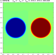
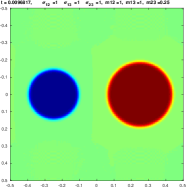
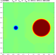
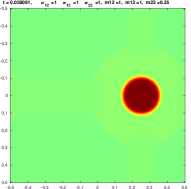
Figure 1. Mean curvature flow of two circular phases, with $\sigma_{12}=\sigma_{13}=\sigma_{23}=1$ and $m_{12}=1$, $m_{13}=1$, $m_{23}=\frac{1}{4}$. The images show the values of the function $2u_{2}+u_{3}$ at different times using a colormap such that $u_{1}$, $u_{2}$, and $u_{3}$ are represented in blue, red and green, respectively.

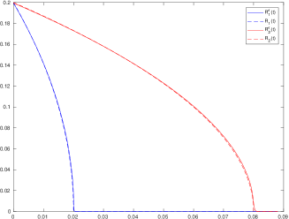
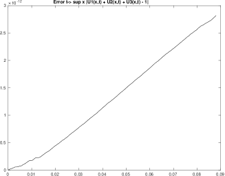
Figure 2. Mean curvature flow of two circular phases. Surface tensions are identical, mobilities are $(m_{12},m_{13},m_{23})=(1,1,\frac{1}{4})$. Left : Comparison of the radii $R_{k}^{\varepsilon}(t)$ and their theoretical values $R_{i}(t)$ associated with the phases $u_{k}$, k=1,2. Right: Plot of $\|1-\sum_{k}u_{k}(.,t)\|_{L^{\infty}}$.

4.2. Influence of the choice of a particular decomposition of mobilities

The decomposition (8) is not unique and it is therefore legitimate to question its effect on the numerical approximation of the flow. We consider here the simplest case using $N=3$ phases, homogeneous surface tensions $\sigma_{i,j}=1$ and homogeneous mobility coefficients $m_{ij}=1$. We then compare the numerical approximations associated with the following decompositions of the mobilities:

• the canonical choice with $P=3$:

  $$(m^{1}_{12},m^{1}_{13},m^{1}_{23})=(1,0,0),\;(m^{2}_{12},m^{2}_{13},m^{2}_{23})=(0,1,0)\;\text{ and }\;(m^{3}_{12},m^{3}_{13},m^{3}_{23})=(0,0,1)$$

  where

  $$(m^{1}_{1},m^{1}_{2},m^{1}_{3})=(2,2,0),\;(m^{2}_{1},m^{2}_{2},m^{2}_{3})=(2,0,2)\;\text{ and }\;(m^{3}_{1},m^{3}_{1},m^{3}_{1})=(0,2,2).$$

• a sparse decomposition with $P=1$:

  $$(1,1,1)=(m_{12},m_{13},m_{23})=\sum_{p=1}^{1}(m^{p}_{12},m^{p}_{13},m^{p}_{23})=(m^{1}_{12},m^{1}_{13},m^{1}_{23}),$$

  where $(m^{1}_{1},m^{1}_{2},m^{1}_{3})=(2,2,2)$. Notice that $(m_{12},m_{13},m_{23})=(1,1,1)$ is indeed harmonically additive which explains why we can use $P=1$.

The following numerical parameters $\varepsilon=1.5/K$, $\delta_{t}=0.25/K^{2}$, and $\alpha=0$ are used. Figure 3 shows the numerical multiphase solution ${\bf u}^{\varepsilon}=(u_{1}^{\varepsilon},u_{2}^{\varepsilon},u_{3}^{\varepsilon})$ at different times. The rows correspond to the canonical and sparse decomposition of the $m_{ij}$’s, respectively . We observe that the two flows are quite similar, which suggests that the choice of a particular decomposition has little influence.

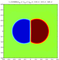
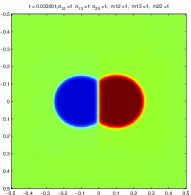
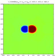
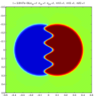
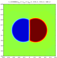
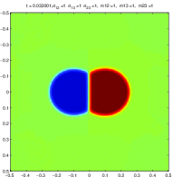
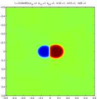
Figure 3. Influence of the choice of a particular decomposition of the mobilities: the canonical decomposition is used on the first row, a sparse decomposition on the second. The images show the values of $2u_{2}+u_{3}$ at different times, with the suitable colormap so that $u_{1}$, $u_{2}$, and $u_{3}$ are represented in blue, red and green, respectively.

4.3. Validation of our approach for highly contrasted mobilities

Our next tests show that our approach can handle highly contrasted mobilities. One expects that when $m_{ij}$ is small (or vanishes) the corresponding interface $\Gamma_{ij}$ hardly moves. The tests also show that mobilities are parameters that may strongly affect the flow. The computations have been performed with $\varepsilon=1/K$, $\delta_{t}=1/K^{2}$, and $\alpha=2$. Figure 4 represents a first series of numerical experiments in which $\sigma_{12}=\sigma_{13}=\sigma_{23}=1$. The rows depict the flow associated with the mobilities $(m_{12},m_{13},m_{23})=(1,1,1)$, $(0,1,1)$, and $(0,1,0)$ respectively, with the same initial condition. On each image, the phases $u_{1}$ and $u_{2}$ are plotted in blue and red respectively. As expected, the blue-red interface $\Gamma_{12}$ does not move when $m_{12}=0$ (second line), or when $m_{23}$ (third line).

Figure 5 represent similar experiments with the non-identical surface tensions $\sigma_{12}=0.1$ and $\sigma_{13}=\sigma_{23}=1$. The same conclusions hold.

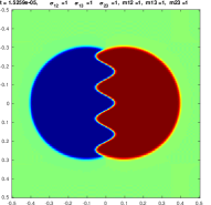
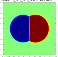
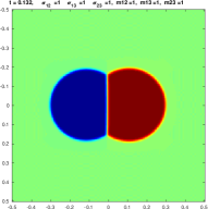
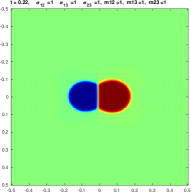
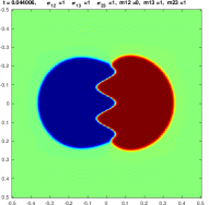
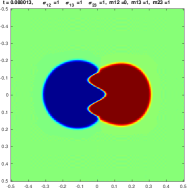
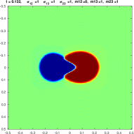
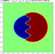
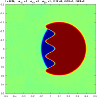
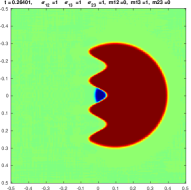
Figure 4. Mean curvature flows with highly contrasted mobilities, identical surface tensions. The rows correspond to $(m_{12},m_{13},m_{23})=(1,1,1)$, $(m_{12},m_{13},m_{23})=(0,1,1)$, and $(m_{12},m_{13},m_{23})=(0,1,0)$, respectively. Images show the values of the function $2u_{2}+u_{3}$ at different times using a colormap such that $u_{1}$, $u_{2}$, and $u_{3}$ appear in blue, red and green, respectively.

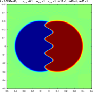
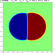
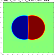
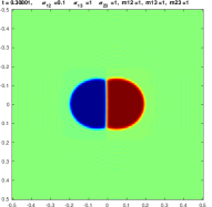
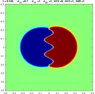
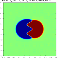
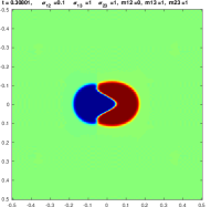
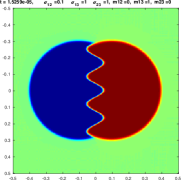
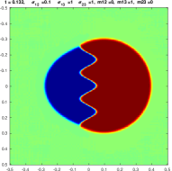
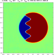
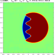
Figure 5. Mean curvature flows with highly contrasted mobilities, non-identical surface tensions. The rows correspond to $(m_{12},m_{13},m_{23})=(1,1,1)$, $(m_{12},m_{13},m_{23})=(0,1,1)$, and $(m_{12},m_{13},m_{23})=(0,1,0)$, respectively. Images show the values of the function $2u_{2}+u_{3}$ at different times using a colormap such that $u_{1}$, $u_{2}$, and $u_{3}$ appear in blue, red and green, respectively.

4.4. Numerical experiments with $N=4$ phases

We show now that our method can handle flows involving more than 3 phases. We consider a configuration with 4 phases and a canonical decomposition of the mobilities ${\bf m}=(m_{12},m_{13},m_{14},m_{23},m_{24},m_{34})$, which takes the form

$$(m_{12},m_{13},m_{14},m_{23},m_{24},m_{34})=\sum_{p=1}^{6}(m^{p}_{12},m^{p}_{13},m^{p}_{14},m^{p}_{23},m^{p}_{24},m^{p}_{34}),$$

where

$$(m^{p}_{12},m^{p}_{13},m^{p}_{14},m^{p}_{23},m^{p}_{24},m^{p}_{34})=\begin{cases}(m_{12},0,0,0,0,0,0)&\text{ if }p=1\\ (0,m_{13},0,0,0,0,0)&\text{ if }p=2\\ \hskip 42.67912pt\vdots&\\ (0,0,0,0,0,0,m_{34})&\text{ if }p=6\\ \end{cases}$$

Figure 6 shows a series of numerical experiments using

$$(\sigma_{12},\sigma_{13},\sigma_{14},\sigma_{23},\sigma_{24},\sigma_{34})=(1,1,1,1,1,1).$$

The rows correspond to ${\bf m}=(1,1,1,1,1,1)$, ${\bf m}=(0,1,1,1,1,1)$, and ${\bf m}=(0,0,1,1,1,1)$, respectively. In each image, the phases $u_{1},u_{2},u_{3},u_{4}$ are depicted in light blue, red, blue, and green, respectively. These results show good agreement with the expected theoretical flows.

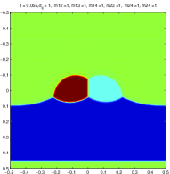
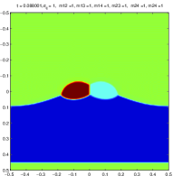
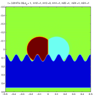
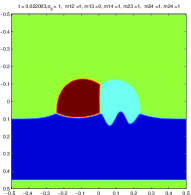
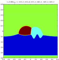
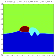
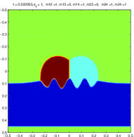
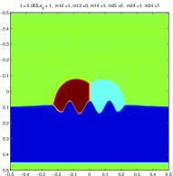
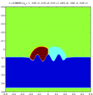
Figure 6. Numerical experiments with $N=4$ phases and homogeneous surface tensions $\sigma_{ij}=1$. The rows correspond to $(m_{12},m_{13},m_{14},m_{23},m_{24},m_{34})$ equal to $(1,1,1,1,1,1)$, $(0,1,1,1,1,1)$, and $(0,0,1,1,1,1)$, respectively. The images represent the values of $u_{1}+3u_{2}+1.5u_{4}$ at different times, with a suitable colormap so that $u_{1}$, $u_{2}$, $u_{3}$, and $u_{4}$ are shown in light blue, red, blue and green, respectively.

4.5. Numerical experiments in dimension $3$

Figure 7 shows the 3D version of the 2D computations reported in Figure 4. The surface tensions are identical, $\sigma_{ij}=1$. The rows represent the evolutions from the same initial condition with mobilities $(m_{12},m_{13},m_{23})$ equal to $(1,1,1)$, $(0,1,1)$, and $(0,1,0)$ respectively. In each image, the phases $u_{1}$ and $u_{2}$ are depicted in blue and red, respectively.

Our last example, shown in Figure 7, concerns a more complex situation with 3 phases where the initial geometry represents a toy truck. We compare evolutions obtained with different sets of mobilities, and with surface tensions $\sigma_{i,j}$ all equal to $1$.

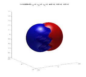
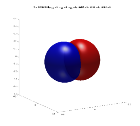
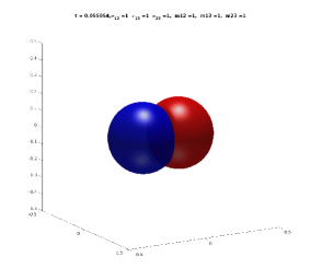
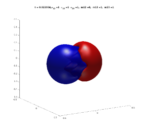
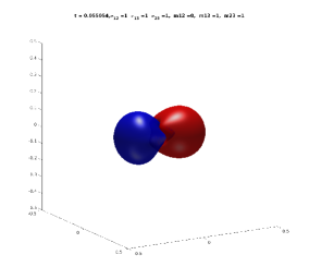
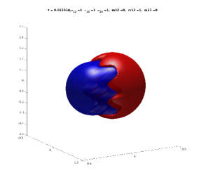
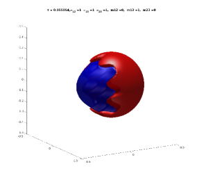
Figure 7. 3D multiphase mean curvature flows with homogeneous surface tensions $\sigma_{12}=\sigma_{13}=\sigma_{23}=1$. The rows correspond to $(m_{12},m_{13},m_{23})=(1,1,1)$, $(m_{12},m_{13},m_{23})=(0,1,1)$, and $(m_{12},m_{13},m_{23})=(0,1,0)$, respectively. The images show the level set $\{u_{1}=1/2\}$ in blue, and the level set $\{u_{2}=1/2\}$ in red, at different times.

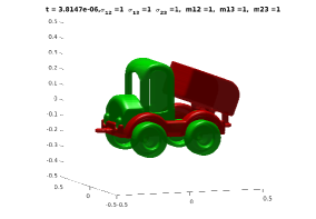
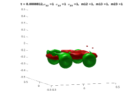
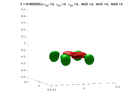
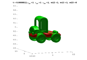
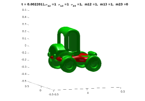
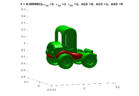
Figure 8. 3D multiphase mean curvature flows with homogeneous surface tensions $\sigma_{12}=\sigma_{13}=\sigma_{23}=1$. The rows correspond to $(m_{12},m_{13},m_{23})=(1,1,1)$, $(m_{12},m_{13},m_{23})=(1,1,0)$, and $(m_{12},m_{13},m_{23})=(0,1,0)$, respectively. The images show the 1/2-level sets of $u_{1}$ (red) and $u_{2}$ (green) at different times.

5. Conclusion

We introduced in this paper a numerical scheme for the approximation of multiphase mean curvature flow with additive surface tensions and general nonnegative mobilities. The scheme uses a decomposition of the set of mobilities as sums of harmonically additive mobilities. We provided a formal asymptotic expansion showing that smooth solutions of the associated Allen-Cahn system approximate a sharp interface motion driven by $V_{ij}=m_{i,j}\sigma_{ij}H_{ij},1\leq i<j\leq N$, up to order 2 in the order parameter $\varepsilon$. The numerical tests we report are consistent with this expected accuracy. In particular, when the contrast between mobilities is large, our scheme provides approximate flows characterized by a width of the diffuse interface between phases that is not affected by the mobility contrast.

References

- [1] S. M. Allen and J. W. Cahn. A microscopic theory for antiphase boundary motion and its application to antiphase domain coarsening. Acta Metall., 27:1085–1095, 1979.
- [2] L. Ambrosio. Geometric evolution problems, distance function and viscosity solutions. In Calculus of variations and partial differential equations (Pisa, 1996), pages 5–93. Springer, Berlin, 2000.
- [3] S. Baldo. Minimal interface criterion for phase transitions in mixtures of cahn-hilliard fluids. Annales de l’institut Henri Poincaré (C) Analyse non linèaire, 7(2):67–90, 1990.
- [4] G. Bellettini. Lecture Notes on Mean Curvature Flow, Barriers and Singular Perturbations. Scuola Normale Superiore, Pisa, 2013.
- [5] G. Bellettini and M. Paolini. Quasi-optimal error estimates for the mean curvature flow with a forcing term. Differential Integral Equations, 8(4):735–752, 1995.
- [6] G. Bellettini and M. Paolini. Quasi-optimal error estimates for the mean curvature flow with a forcing term. Differential Integral Equations, 8(4):735–752, 1995.
- [7] M. Ben Said, M. Selzer, B. Nestler, D. Braun, C. Greiner, and H. Garcke. A phase-field approach for wetting phenomena of multiphase droplets on solid surfaces. Langmuir, 30(14):4033–4039, 2014. PMID: 24673164.
- [8] J. Bence, B. Merriman, and S. Osher. Diffusion generated motion by mean curvature. Computational Crystal Growers Workshop,J. Taylor ed. Selected Lectures in Math., Amer. Math. Soc., pages 73–83, 1992.
- [9] E. Bonnetier, E. Bretin, and A. Chambolle. Consistency result for a non monotone scheme for anisotropic mean curvature flow. Interfaces Free Bound., 14(1):1–35, 2012.
- [10] E. Bonnetier and A. Chambolle. Computing the equilibrium configuration of epitaxially strained crystalline films. SIAM J. Appl. Math., 62(4):1093–1121, 2002.
- [11] M. Brassel and E. Bretin. A modified phase field approximation for mean curvature flow with conservation of the volume. Mathematical Methods in the Applied Sciences, 34(10):1157–1180, 2011.
- [12] E. Bretin, A. Danescu, J. Penuelas, and S. Masnou. Multiphase mean curvature flows with high mobility contrasts: A phase-field approach, with applications to nanowires. Journal of Computational Physics, 365:324 – 349, 2018.
- [13] E. Bretin, R. Denis, J.-O. Lachaud, and E. Oudet. Phase-field modelling and computing for a large number of phases. ESAIM Math. Model. Numer. Anal., 53(3):805–832, 2019.
- [14] E. Bretin and S. Masnou. A new phase field model for inhomogeneous minimal partitions, and applications to droplets dynamics. Interfaces and Free Boundaries, 2017.
- [15] G. Caginalp and P. C. Fife. Dynamics of layered interfaces arising from phase boundaries. SIAM J. Appl. Math., 48(3):506–518, 1988.
- [16] J. W. Cahn. Critical point wetting. The Journal of Chemical Physics, 66(8):3667–3672, 1977.
- [17] L. Chen and J. Shen. Applications of semi-implicit Fourier-spectral method to phase field equations. Computer Physics Communications, 108:147–158, 1998.
- [18] X. Chen. Generation and propagation of interfaces for reaction-diffusion equations. J. Differential Equations, 96(1):116–141, 1992.
- [19] P. de Mottoni and M. Schatzman. Geometrical evolution of developed interfaces. Trans. Amer. Math. Soc., 347:1533–1589, 1995.
- [20] D. Eyre. Computational and mathematical models of microstructural evolution,. Warrendale:The Material Research Society, 1998.
- [21] H. Garcke, B. Nestler, and B. Stoth. On anisotropic order parameter models for multi-phase systems and their sharp interface limits. Physica D: Nonlinear Phenomena, 115(1-2):87 – 108, 1998.
- [22] H. Garcke, B. Nestler, and B. Stoth. A multi phase field concept: Numerical simulations of moving phase boundaries and multiple junctions. SIAM J. Appl. Math, 60:295–315, 1999.
- [23] H. Garcke, B. Nestler, and B. Stoth. A multiphase field concept: numerical simulations of moving phase boundaries and multiple junctions. SIAM J. Appl. Math., 60(1):295–315, 2000.
- [24] D. Gilbarg and N. Trudinger. Elliptic Partial Differential Equations of Second Order. Springer, 1998.
- [25] P. Loreti and R. March. Propagation of fronts in a nonlinear fourth order equation. European Journal of Applied Mathematics, 11:203–213, 3 2000.
- [26] L. Modica and S. Mortola. Un esempio di -convergenza. Boll. Un. Mat. Ital. B (5), 14(1):285–299, 1977.
- [27] W. W. Mullins. Two-Dimensional Motion of Idealized Grain Boundaries, pages 70–74. Springer Berlin Heidelberg, Berlin, Heidelberg, 1999.
- [28] E. Oudet. Approximation of partitions of least perimeter by Gamma-convergence: around Kelvin’s conjecture. Experimental Mathematics, 20(3):260–270, 2011.
- [29] R. L. Pego. Front migration in the nonlinear Cahn-Hilliard equation. Proc. Roy. Soc. London Ser. A, 422(1863):261–278, 1989.
- [30] S. J. Ruuth. Efficient algorithms for diffusion-generated motion by mean curvature. J. Comput. Phys., 144(2):603–625, 1998.
- [31] J. Shen, C. Wang, X. Wang, and S. M. Wise. Second-order convex splitting schemes for gradient flows with ehrlich-schwoebel type energy: Application to thin film epitaxy. SIAM J. Numerical Analysis, 50(1):105–125, 2012.
- [32] K. Takasao. Convergence of landau-lifshitz equation to multi-phase brakke’s mean curvature flow. preprint.
- [33] N. Wang, M. Upmanyu, and A. Karma. Phase-field model of vapor-liquid-solid nanowire growth. Phys. Rev. Materials, 2:033402, Mar 2018.