Implicit Riemannian Concave Potential Maps
Abstract
We are interested in the challenging problem of modelling densities on Riemannian manifolds with a known symmetry group using normalising flows. This has many potential applications in physical sciences such as molecular dynamics and quantum simulations. In this work we combine ideas from implicit neural layers and optimal transport theory to propose a generalisation of existing work on exponential map flows, Implicit Riemannian Concave Potential Maps, IRCPMs. IRCPMs have some nice properties such as simplicity of incorporating symmetries and are less expensive than ODE-flows. We provide an initial theoretical analysis of its properties and layout sufficient conditions for stable optimisation. Finally, we illustrate the properties of IRCPMs with density estimation experiments on tori and spheres.
1 Introduction
This work focuses on applications of generative models where we want to approximate a -invariant target density , , with support on a prescribed compact Riemannian manifold and a known isometry group . This setting is important to many applications of ML to physical systems such as molecular systems [KKN20, WBP+20, NOKW19] and quantum field theory simulations [KAB+20, BKR+21].
To achieve this, we aim to build generative models with support on whose density is -invariant by construction (as opposed to learning an approximate -invariance). We focus on a family of models termed normalising flows. These are generative models whose density is defined via the push-forward of a base density through a parametric diffeomorphism with parameters (usually parametrised by a neural network), [PNR+19]. Normalising flows can be used to construct -invariant densities when the base density is -invariant (e.g. the Haar measure) and the diffeomorphism is -equivariant. This mechanism has been used to build invariant models on Euclidean manifolds [RRHT19, PNR+19, KKN20], Lie groups (U, SU) [KAB+20, BKR+21] and more general manifolds [KLL+21].
We turn our attention to normalising flows built from the gradients of a scalar potential . In the Euclidean space, this family of flows (referred to as convex potential flows, CPFs), where a diffeomorphism is defined via the gradients of a convex potential, 111Convexity of the smooth function on a convex support is a sufficient condition for the map to be a diffeomorphism on the same support. was explored in [HCTC21]. A promising way to extend CPFs to more general Riemannian manifolds builds on results from optimal transport (OT) theory [Vil09, McC01] using cost-convex/concave potentials, which are a natural generalisation of convex/concave potentials in the Euclidean space. This has been explored in [Sei13, CAL21, RRHT19].
A cost-concave (c-concave) potential with cost is a function that is not identically for which there exists a dual function such that
| (1) |
As observed in [CAL21] when is a smooth Riemannian manifold, OT theory has a powerful result that given two measures , on , with being absolutely continuous with respect to the volume-measure on and a cost with , where is the geodesic distance, there is a unique -concave potential that minimises such that is the push-forward of through the diffeomorphism , where is the Riemannian exponential map at the point and is the covariant derivative at , [McC01, Theorem 9] and [Vil09, Corollary 10.44]. This result gives us the confidence that, if we can parametrise a sufficiently expressive family of c-concave potentials, it is possible to approximate an arbitrary target measure starting from a simple base measure . In what follows we will only consider the case .
In this paper we explore normalising flows constructed from the exponential map of the gradients of cost-concave potentials as outlined above, building on work from [Sei13, CAL21, RRHT19]. Our contributions are as follows:
-
1.
We introduce Implicit Riemannian Concave Potential Maps, IRCPMs which extend Riemannian Convex Potential Maps, RCPMs from [CAL21] by allowing for much more general c-concave functions, Section 3.1, and by making it easy to incorporate symmetries of the target density, Section 3.2;
-
2.
We extend results from implicit layers, [ZGM+20, AK17], allowing higher-order implicit derivatives to be efficiently computed, Section 4.2;
- 3.
Finally we provide proof-of-concept experimental results on toy densities on tori in Section 5.1 and spheres in Section 5.2.
2 Related Work
Previous work [Sei13, RPR+20] has focused on directly parametrising the c-concave function with a neural network or other parametric family. This has the advantage of allowing a closed form flow, but it is hard to implement general and expressive solutions. Even for simple manifolds such as spheres, this proves to be a challenge [RPR+20, CAL21].
Discrete c-concave potential flows are a manifold-agnostic solution to parametrise c-concave functions whose dual function is assumed to be discrete. This reduces the continuous minimisation in Equation 1 to taking the minimum over a discrete set of values, [CAL21]. While this solution can be shown to enjoy universal approximation properties, it still has two main issues that we wish to address: (i) Scaling issues to high-dimensions (since discrete c-concave potentials are like mixture models it is hard to scale them to large-dimensional spaces without resorting to auto-regressive architectures)222Universality of discrete c-concave potentials relies on using -nets which is a set of points on such that any two points in the set are at most -away from each other. The number of points in the -net grows as , where is the dimension of .; (ii) Difficulty of incorporating target symmetries (there is no computationally cheap mechanism to incorporate known symmetries of the target density into discrete c-concave potentials).
We aim to address issues (i) and (ii) by introducing implicit c-concave potentials, which allow us to work with a much broader family of smooth dual functions , while making it straightforward to incorporate target symmetries, Section 3.2.
Implicit components for neural networks, defined via an inner optimisation, have been explored in many different contexts [BPRS18]; they have been proposed as layers [ZGM+20, AK17], in meta-learning [LMRS19], generative models [KWM+18] and planning [dABPSA+18, SJA+18] to name a few applications.
In [ZGM+20, AK17] implicit layers defined via minimisation or fixed-point equations have been studied. The first-order gradients of implicit layers are computed using the implicit function theorem for efficiency. Our formulation follows the same principles, but we extend the methodology to compute up to third-order gradients efficiently as necessary for our application, Section 4.2.
Equivariant manifold flows [KLL+21] are a general solution to build -equivariant ODE flows on manifolds. Working with ODEs in manifolds introduces several technical challenges such as complex integration procedures and computationally expensive estimation of the model’s likelihood.
OptimalTransport-Flows [OFLR21] are ODE-flows defined in the Euclidean space with additional transport costs added during optimisation.
3 Implicit Riemannian Concave Potential Maps, IRCPMs
3.1 Implicit c-concave functions with NNets
Inspired by the discrete cost-concave potentials proposed in [CAL21] and work on implicit neural layers (i.e. layers whose output is defined via an inner optimisation) [ZGM+20, AK17], we want to explore more general c-concave functions on a manifold by working directly with its definition, Equation 1, as a minimisation problem. We use neural networks to parametrise a family of functions , and implicitly define the function via the minimisation
| (2) |
where . The implicit c-concave function is then used to define a normalising flow via
| (3) |
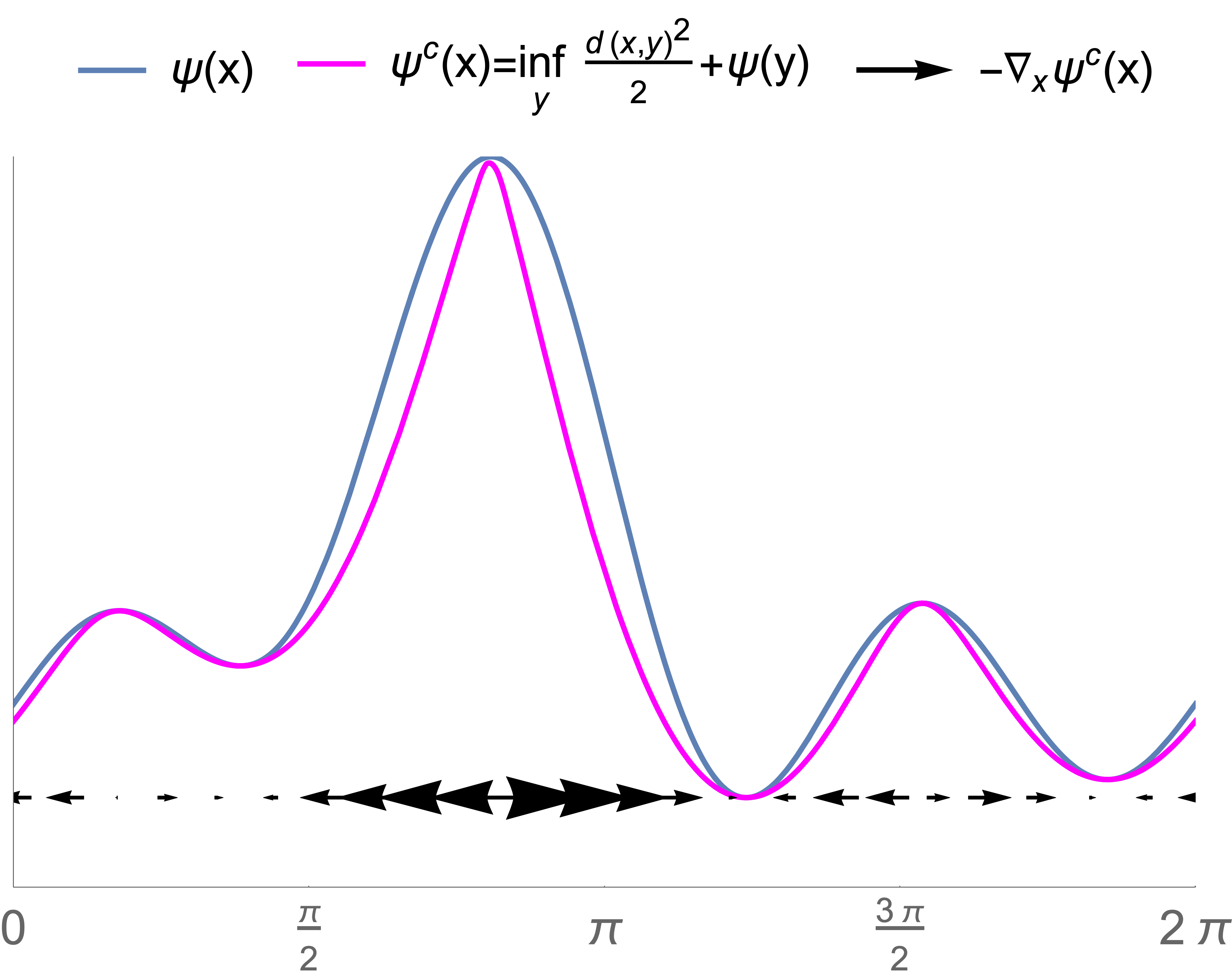
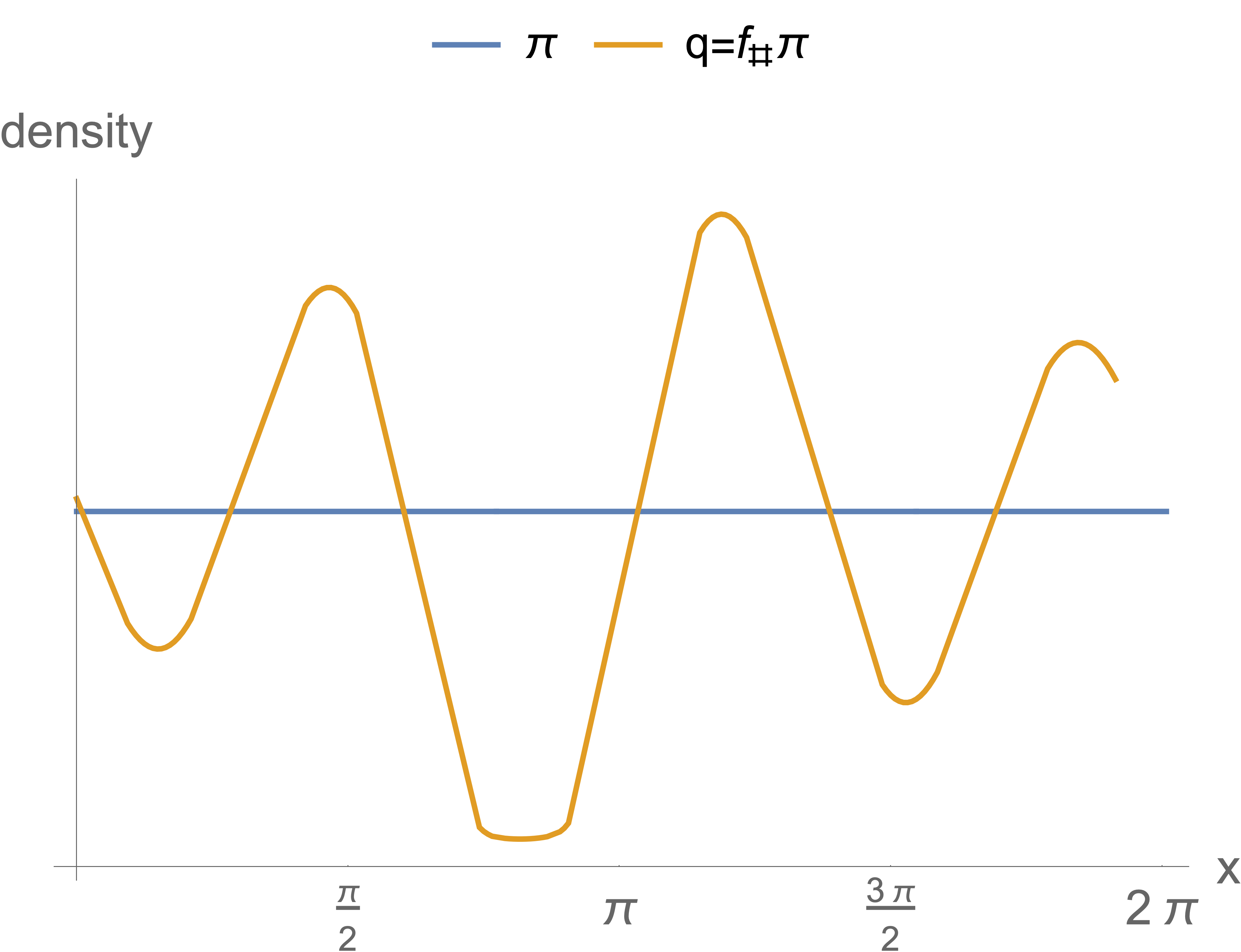
This flow is illustrated in Figure 1(left), where we show a concrete example of , and on the torus . The model’s density is defined via the push-forward of a simple base measure (such as the Haar measure if is a Lie group),
| (4) |
where is the Jacobian matrix of and is a matrix that projects to the tangent space at (this projection is necessary when working with an embedding of into instead of a local chart). In what follows we will refer to this family of normalising flows as implicit Riemannian concave potential maps, IRCPMs.
3.2 Incorporating symmetries
One of the main motivations of this work is to easily incorporate symmetries into our models. Symmetries are described by a group of isometries of the manifold .
We could consider a G-invariant extension of discrete c-concave potentials [CAL21] via the modification
| (5) |
where is the Riemannian distance between the point and the orbit of the point under the action of the symmetry group , . Unfortunately, there is no simple closed-formula for on interesting settings (e.g. quantum simulations on a lattice) which makes this impractical.
We show in 1 that it is relatively simple to build G-equivariant IRCMPs: it is sufficient that (i) the group action is an isometry (i.e. leaves the intrinsic distance function invariant) and (ii) that the function is -invariant.
Lemma 1.
Let be a Riemannian manifold with distance and isometry group ; and let be a G-invariant scalar function. Then the diffeomorphism defined via is G-equivariant.
Proof.
First we show that the cost-concave dual function is G-invariant
| is an isometry with adjoint | ||||
| is invariant | ||||
| is invertible | ||||
It remains to show that is -equivariant if is -invariant. As observed in [KLL+21](Th1) the gradient of a G-invariant scalar function is G-equivariant. Therefore the term is G-equivariant. Finally, the exponential map is equivariant to isometries. Indeed, if , and , the two curves and are two geodesics with and . These two geodesics are therefore equal. Evaluating them at gives us the equivariance of . ∎
3.3 Relation between ,
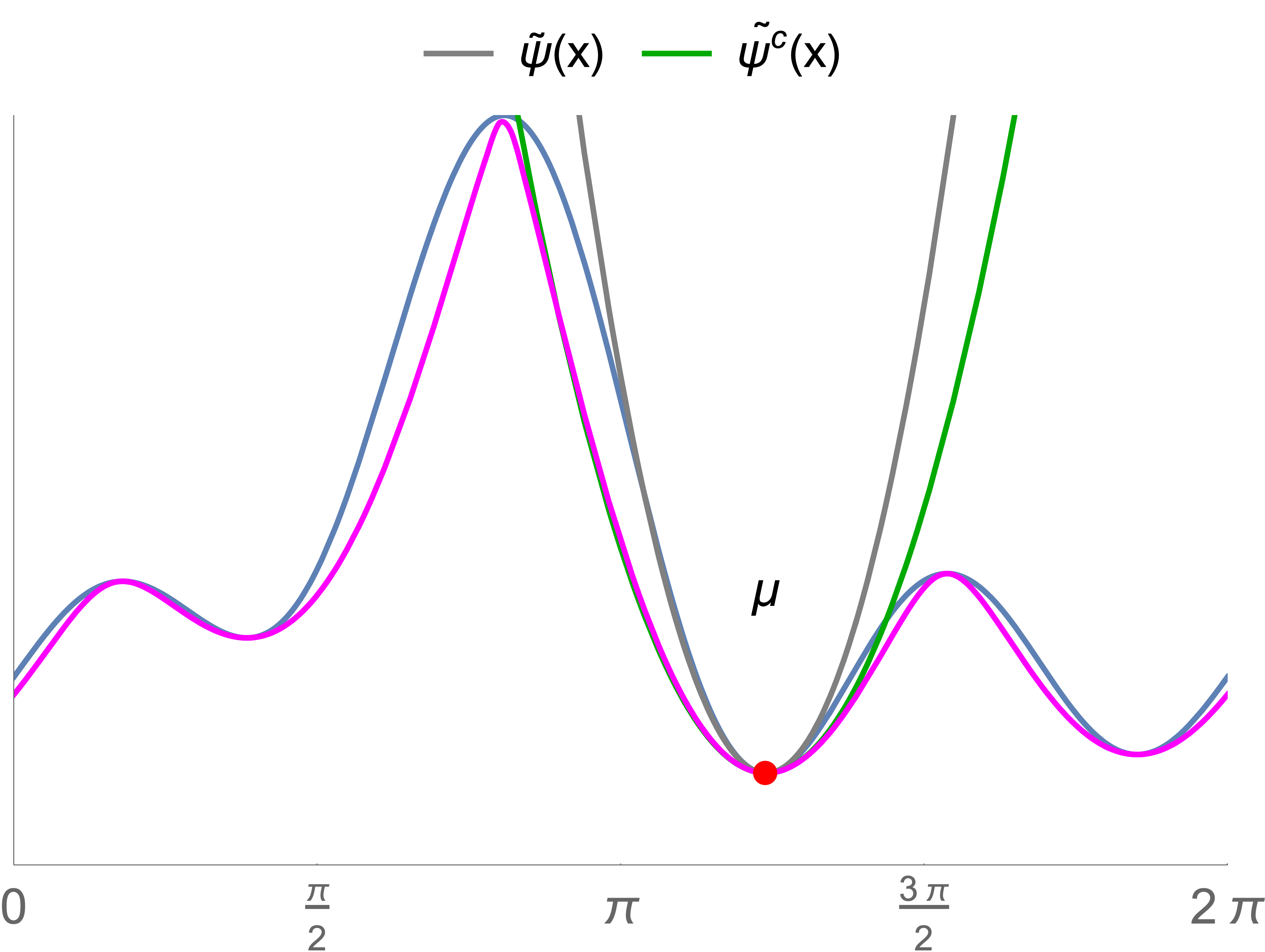
An interesting observation is that local minima of are also local minima of , as formalised in 2 in the Euclidean space. Additionally, 2 relates the Hessian, , of and of at the local minima. Although this observation is limited to Euclidean geometry it suggests that for points near the local minima of the flow will increase the concentration of the base density in the regions . Consequently, and should have a similar local minima structure as the target energy. This suggests a heuristic to initialise as a function of the form , where is the target energy, is a learned non-decreasing function and is a learned "correction". This relationship between and is illustrated in Figure 1(right) using an example and defined on the torus .
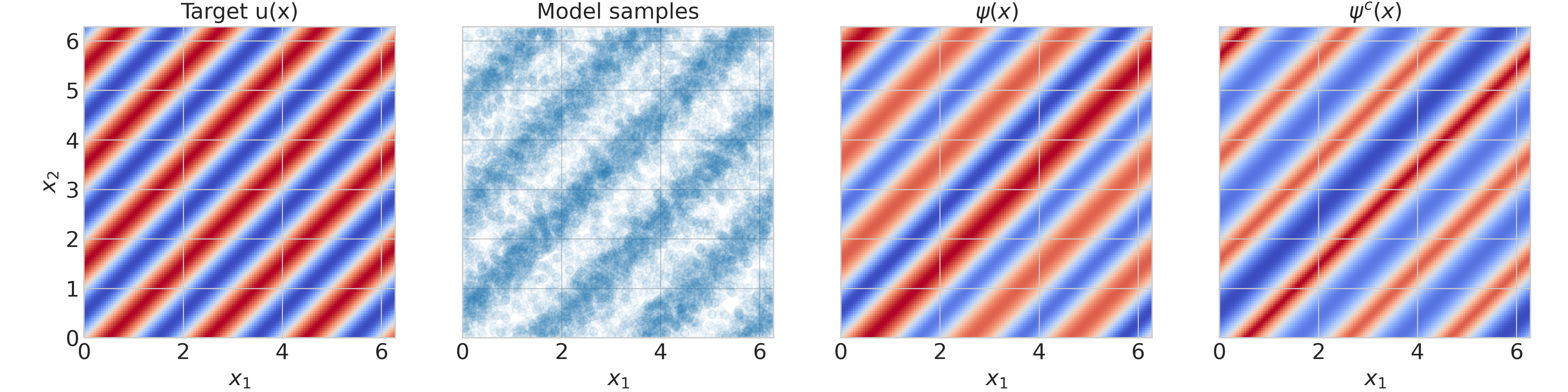
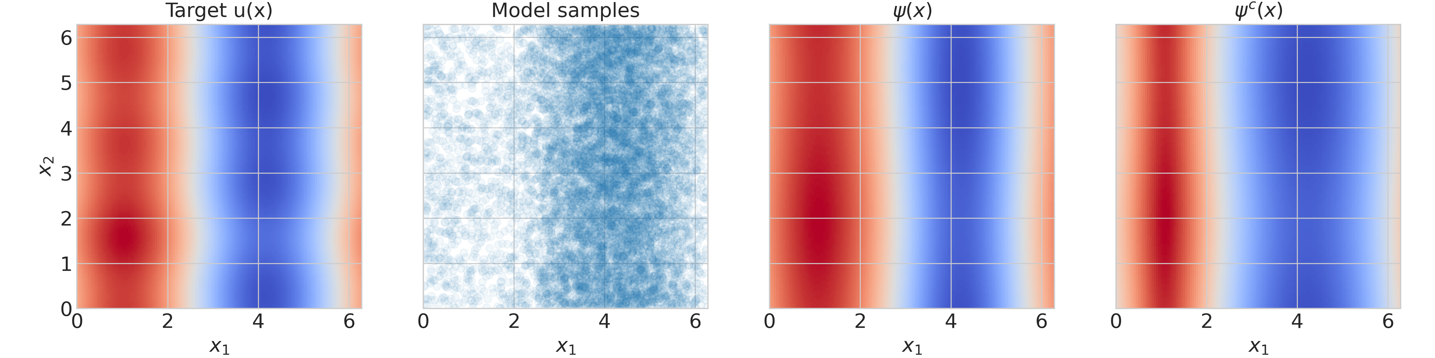
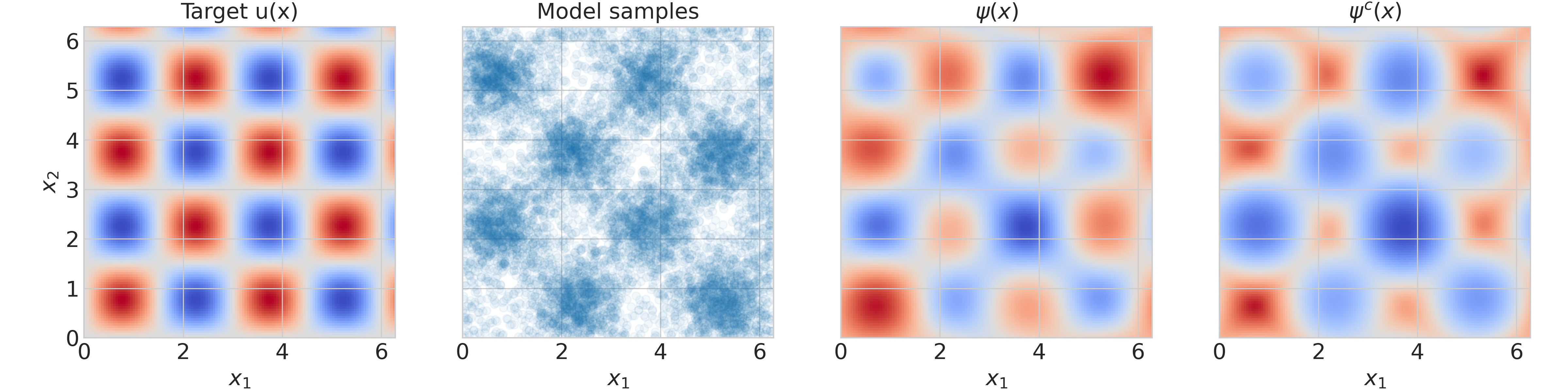
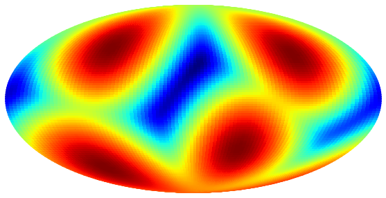
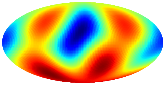
We can empirically observe these relationships in Figure 2 and Figure 3(c) where the learned functions and , develop the same modes as the target density.
Lemma 2.
Let and be a positive definite matrix and . Then the c-concave function dual to is given by
Proof.
Since is assumed positive definite, has a global minimum which is given by solving . We can re-arrange the terms of to a more convenient form by performing a Taylor expansion around up to second-order (since is quadratic, the expansion is exact),
Replacing above gives
Now we note that in the quadratic form above , so it is a quadratic form centred at with Hessian matrix , so it can be re-written as
∎
4 Solving the infimum problem
Given a generic , computing can be a difficult problem. We are interested in finding conditions on which guarantee this problem can be solved with gradient descent.
4.1 Bounding the derivatives of
Let be the function obtained by following gradient descent along on , initialised at . Computing is a much simpler problem than . Below we will see that by controlling the norm of the gradient of , as well as the operator norm of its Hessian, we can guarantee that everywhere.
First, let’s see how to ensure that the global minimum is in a ball around .
Lemma 3.
Assume is such that everywhere, then if we have . In particular, the infimum in of is within a ball of radius around .
Proof.
Let be such that . Since is complete, there exists with and . For , let .
We have
| (6) |
We have . This means . Since the function is positive for , the result follows.
∎
The above Lemma 3 lets us constrain the location of the global minimum inside a ball. Let’s now see a condition to ensure that this minimum is unique inside this ball, and is reached by gradient descent. We write for the Hessian of , and for the operator norm of .
Lemma 4.
We can choose and such that if and everywhere, then for any , has its global minimum within the ball . Gradient descent along on , initialised at , finds this minimum. In other words, .
Proof.
Assume that is small enough such that for any in , the map is a diffeomorphism from the euclidean unit closed ball in onto its image . Also, as in Lemma 3, assume that everywhere.
Since is a sum of two terms, and , its Hessian with respect to is also a sum of two terms, respectively and . At , the Hessian is exactly the identity . This means that for any in , if is small enough, then in . Now, assume that everywhere. This implies that and is invertible with eigenvalues in . In particular it is positive definite at any in . We can immediately conclude from [Mil16, Lemma 2.2] that critical points of are all isolated minima inside . The vector field along the boundary of points strictly inward the ball. By [JJ08, Cor. 8.3.1], the ball is the disjoint union of its stable manifolds 333A stable manifold of a critical point is the set of points on the manifold for which the integral curves of converge to at goes to . The dimension of this manifold is given by the number of positive eigenvalues of the Hessian at the critical point . See [JJ08] for more details., where runs over all the critical points of . Since at every critical points of the Hessian is positive definite, all the submanifolds are open and of the same dimension as . Since is connected, there is only one critical point and . By definition of , gradient descent along leads to . ∎
4.2 Implicit higher-order gradients
From 4, under Lipschitz constraints on and its gradients, the global minimum in Equation 1 will coincide with the local minima . This allows us to formulate Equation 2 as an equality constraint implicit layer [ZGM+20, AK17], , where
| (7) |
The first-order gradients of the minimiser with respect to can be efficiently computed via the implicit function theorem.
IRCPMs are built using the first-order gradients of , which require first-order gradients of with respect to . As a consequence, the log-det-Jacobian terms in Equation 4 will involve second-order derivatives of with respect to . Finally, optimisation of the model’s likelihood will require computing an extra derivative with respect to the model’s paramters . This results in third-order derivatives of (second-order in and an extra derivative with respect to ).
We can efficiently compute higher-order derivatives of with respect to and by considering a recursive computation of vector-Jacobian products . As in [ZGM+20, AK17], are obtained by solving a linear system of equations
| (8) |
Second and higher-order vector-Jacobian products can be obtained by a recursive application of Equation 8. More precisely, let the -th order vector-Jacobian product be . If is implicitly defined via the (linear) equality constraint then, the -th order vector-Jacobian product is given by .
4.3 The case of
The Hessian of the squared distance, as well as its eigenvalues, is computed in [FX06, Pen17]. Using this, we will offer practical choices for and .
5 Optimisation and Experiments
In each experiment we trained the model to approximate a given target density for some energy function defined either on a torus or on the sphere . The model used for the experiments is either an IRCPM or a stack of IRCPMs as specified in each experiment.
The function is parametrised with a two-layer MLP with softplus non-linearities with layer sizes [32, 32, 1] for the experiments on the torus and layer sizes [128, 128, 1] for the experiments on the sphere. The parameters of are optimised using the Adam optimiser [KB14] to minimise the KL-divergence between the density defined by the model and the target ,
| (9) |
where is the normaliser of the target density. The gradients of the term with respect to are estimated using the stochastic estimator from [DEN+17, HCTC21] unless stated otherwise. For all experiments we report estimated values of and the effective sample size (ESS), [DDFG01, LL01], using samples from the model.
5.1 Targets on
We tested IRCPMs on 3 target densities on the torus . Their expressions are detailed in Table 1. These targets test the ability of our model to capture modes as well as to incorporate symmetries. For the experiment with symmetries the target has a continuous symmetry group for some arbitrary angle . The symmetry was exactly incorporated into the model by using invariant features as input to the function , this architecture is referred to as "Symmetric MLP" in Table 1. The results are shown in Figure 2 and Table 1. In all cases the model reaches ESS . We observed, as suggested by the analysis in Section 3.3, that the learned function has similar mode structure as the target energy.
In Table 1 we compared a free form (parametrised by a neural network) with different parametrisations inspired by Section 3.3 which use the target energy to construct in a way that leverages its local structure. The experiments suggest that combining learned components with the target energy while preserving its mode structure allows the model to reach competitive ESS while using a much smaller number of parameters, which is a very desirable property.
| Target | architecture | # parameters | ESS |
|---|---|---|---|
| MLP | 1249 | ||
| Symmetric MLP | 1249 | ||
| 1 | |||
| 4 | |||
| as in [RPR+20, Table 2, multi-modal] | MLP | 1249 | |
| 1 | |||
| 4 | |||
| MLP | 1249 | ||
| 1 | |||
| 4 |
5.2 Multi-modal target on
We tested our setup on the sphere by choosing a target density from [RPR+20], which was also used in [CAL21]. The target is a mixture of the form
| (10) |
where , , , , maps from spherical to Euclidean coordinates, and is a point on the embedded sphere in Euclidean coordinates.
Our model consists of a stack of three IRCPMs with shared parameters, as we found that stacking the same transformation lead to more stable training. The neural network is an MLP that takes the euclidean coordinates of points in as inputs. The output of the MLP is divided by , which is equivalent to initialising the weights of the last layer of the MLP closer to . We also found this to help with training stability and final performance. Finally, we computed the logarithmic determinant of the Jacobian exactly inside the KL, and did not need stochastic estimators of the gradients.
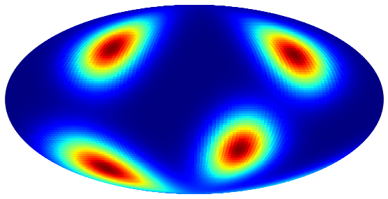
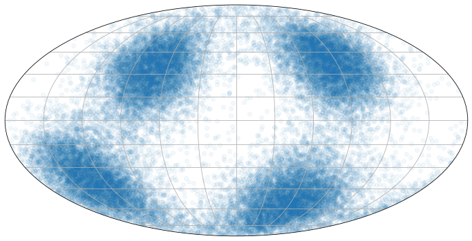
The performance of our model is on par with the RCPM model of [CAL21], with an ESS above and a KL of around nats. Figure 3(c) shows the learnt . Note how the modes of are placed nearby the modes of the target density in Fig. 3(a).
We checked that the bounds derived in Sections 4.3 are satisfied by our trained model. For this purpose, we sampled a million points uniformly at random on , and computed the norm of the gradient of as well as the operator norm of the Hessian . We observed , and . Since , our model sits comfortably within the bounds derived in Section 4.3 and we conclude that it is safe to use gradient descent to find .
Given the success of simpler models and on the torus, Table 1, we tried those same models on . Despite the qualitative similarity between Fig 3(c) and the target energy Fig 3(b) of our trained MLP model, we found the simpler models to be unstable and not competitive so more work is needed to take advantage of the similarities between and . Finally, we trained a model with a single or only stacked transformations instead of as above. We found the models with stack height or to be qualitatively equivalent: scatter plots, as well as ESS and KL were indistinguishable. The only difference was that with only stacked transformations, we observed and . These values are too high and do not satisfy the bounds of Section 4.3. This suggests that the bounds of that section might be too restrictive, and future work could improve on them. With a single transformation, the values of measured during training were even higher. Training of the model was unstable, with only some seeds reaching high ESS, while for other the ESS initially rose before collapsing.
6 Discussion
We introduced Implicit Riemannian Concave Potential Maps, IRCPMs. A class of normalising flow models that uses implicit layers (that is, layers defined via a minimum problem) to define cost-concave potentials for exponential map flows. It extends prior work [CAL21] by considering a more general class of cost-concave functions, which allow for easy incorporation of known symmetries of the target density. We provided an initial theoretical analysis of the proprieties of these flows and lay-ed out conditions for stable training. In particular, the relationship between and the target energy is very intriguing. If we can better understand this relationship, perhaps we’ll be able to come up with more effective parametrisation of .
Similarly to other recent work on flows on Riemannian manifolds [CAL21, KLL+21], the model definition is agnostic to the underlying manifold structure, but its practical implementation requires the ability to efficiently compute the exponential map, covariant derivatives and geodesic distances.
IRCPMs have no explicit formula for the log-det-Jacobian terms. It therefore relies on stochastic estimators for scalable training [DEN+17, HCTC21] but evaluation of such models in high-dimensional settings based on exact likelihoods is still a challenge. This challenge is common to all flow models without explicit log-det-Jacobian [PNR+19, GCB+18, CAL21, KLL+21, MN20] and not specific to our proposed model.
The presented experiments are only to provide an illustration and proof-of-concept of different aspects of IRCPMs. Since the target manifolds are low-dimensional and the neural networks used are relatively small, we used a naive backpropagation through the minimisation in Equation 2 for optimisation. However we emphasise that a much more scalable training can be performed using the implicit higher-order gradients from Section 4.2 (both in terms of memory and compute).
References
- [AK17] Brandon Amos and J. Zico Kolter. OptNet: Differentiable optimization as a layer in neural networks. In Proceedings of the 34th International Conference on Machine Learning, volume 70 of Proceedings of Machine Learning Research, pages 136–145. PMLR, 2017.
- [BKR+21] Denis Boyda, Gurtej Kanwar, Sébastien Racanière, Danilo Jimenez Rezende, Michael S Albergo, Kyle Cranmer, Daniel C Hackett, and Phiala E Shanahan. Sampling using su (n) gauge equivariant flows. Physical Review D, 103(7):074504, 2021.
- [BPRS18] Atilim Gunes Baydin, Barak A Pearlmutter, Alexey Andreyevich Radul, and Jeffrey Mark Siskind. Automatic differentiation in machine learning: a survey. Journal of machine learning research, 18, 2018.
- [CAL21] Samuel Cohen*, Brandon Amos*, and Yaron Lipman. Riemannian Convex Potential Maps. In ICML, 2021.
- [dABPSA+18] Filipe de Avila Belbute-Peres, Kevin Smith, Kelsey Allen, Josh Tenenbaum, and J Zico Kolter. End-to-end differentiable physics for learning and control. Advances in neural information processing systems, 31:7178–7189, 2018.
- [DDFG01] Arnaud Doucet, Nando De Freitas, and Neil Gordon. An introduction to sequential monte carlo methods. In Sequential Monte Carlo methods in practice, pages 3–14. Springer, 2001.
- [DEN+17] Kun Dong, David Eriksson, Hannes Nickisch, David Bindel, and Andrew Gordon Wilson. Scalable log determinants for gaussian process kernel learning. arXiv preprint arXiv:1711.03481, 2017.
- [FX06] Ricardo Ferreira and Joao Xavier. Hessian of the riemannian squared distance function on connected locally symmetric spaces with applications. In Controlo 2006, 7th Portuguese conference on automatic control, volume 2. Citeseer, 2006.
- [GCB+18] Will Grathwohl, Ricky TQ Chen, Jesse Bettencourt, Ilya Sutskever, and David Duvenaud. Ffjord: Free-form continuous dynamics for scalable reversible generative models. arXiv preprint arXiv:1810.01367, 2018.
- [HCTC21] Chin-Wei Huang, Ricky T. Q. Chen, Christos Tsirigotis, and Aaron Courville. Convex potential flows: Universal probability distributions with optimal transport and convex optimization. In International Conference on Learning Representations, 2021.
- [JJ08] Jürgen Jost and Jeurgen Jost. Riemannian geometry and geometric analysis, volume 42005. Springer, 2008.
- [KAB+20] Gurtej Kanwar, Michael S Albergo, Denis Boyda, Kyle Cranmer, Daniel C Hackett, Sébastien Racaniere, Danilo Jimenez Rezende, and Phiala E Shanahan. Equivariant flow-based sampling for lattice gauge theory. Physical Review Letters, 125(12):121601, 2020.
- [KB14] Diederik P Kingma and Jimmy Ba. Adam: A method for stochastic optimization. arXiv preprint arXiv:1412.6980, 2014.
- [KKN20] Jonas Köhler, Leon Klein, and Frank Noé. Equivariant flows: exact likelihood generative learning for symmetric densities. In International Conference on Machine Learning, pages 5361–5370. PMLR, 2020.
- [KLL+21] Isay Katsman, Aaron Lou, Derek Lim, Qingxuan Jiang, Ser-Nam Lim, and Christopher De Sa. Equivariant manifold flows. In ICML Workshop on Invertible Neural Networks, Normalizing Flows, and Explicit Likelihood Models, 2021.
- [KWM+18] Yoon Kim, Sam Wiseman, Andrew Miller, David Sontag, and Alexander Rush. Semi-amortized variational autoencoders. In International Conference on Machine Learning, pages 2678–2687. PMLR, 2018.
- [LL01] Jun S Liu and Jun S Liu. Monte Carlo strategies in scientific computing, volume 10. Springer, 2001.
- [LMRS19] Kwonjoon Lee, Subhransu Maji, Avinash Ravichandran, and Stefano Soatto. Meta-learning with differentiable convex optimization. In Proceedings of the IEEE/CVF Conference on Computer Vision and Pattern Recognition, pages 10657–10665, 2019.
- [McC01] Robert J McCann. Polar factorization of maps on riemannian manifolds. Geometric & Functional Analysis GAFA, 11(3):589–608, 2001.
- [Mil16] John Milnor. Morse Theory.(AM-51), Volume 51. Princeton university press, 2016.
- [MN20] Emile Mathieu and Maximilian Nickel. Riemannian continuous normalizing flows. arXiv preprint arXiv:2006.10605, 2020.
- [NOKW19] Frank Noé, Simon Olsson, Jonas Köhler, and Hao Wu. Boltzmann generators: Sampling equilibrium states of many-body systems with deep learning. Science, 365(6457), 2019.
- [OFLR21] Derek Onken, Samy Wu Fung, Xingjian Li, and Lars Ruthotto. Ot-flow: Fast and accurate continuous normalizing flows via optimal transport. In Proceedings of the AAAI Conference on Artificial Intelligence, volume 35, pages 9223–9232, 2021.
- [Pen17] Xavier Pennec. Hessian of the riemannian squared distance. Preprint. https://www-sop.inria.fr/members/Xavier.Pennec/AOS-DiffRiemannianLog.pdf, 2017.
- [PNR+19] George Papamakarios, Eric Nalisnick, Danilo Jimenez Rezende, Shakir Mohamed, and Balaji Lakshminarayanan. Normalizing flows for probabilistic modeling and inference. arXiv preprint arXiv:1912.02762, 2019.
- [RPR+20] Danilo Jimenez Rezende, George Papamakarios, Sébastien Racanière, Michael Albergo, Gurtej Kanwar, Phiala Shanahan, and Kyle Cranmer. Normalizing flows on tori and spheres. In International Conference on Machine Learning, pages 8083–8092. PMLR, 2020.
- [RRHT19] Danilo Jimenez Rezende, Sébastien Racanière, Irina Higgins, and Peter Toth. Equivariant hamiltonian flows. arXiv preprint arXiv:1909.13739, 2019.
- [Sei13] Tomonari Sei. A jacobian inequality for gradient maps on the sphere and its application to directional statistics. Communications in Statistics-Theory and Methods, 42(14):2525–2542, 2013.
- [SJA+18] Aravind Srinivas, Allan Jabri, Pieter Abbeel, Sergey Levine, and Chelsea Finn. Universal planning networks: Learning generalizable representations for visuomotor control. In International Conference on Machine Learning, pages 4732–4741. PMLR, 2018.
- [Vil09] Cédric Villani. Optimal transport: old and new, volume 338. Springer, 2009.
- [WBP+20] Peter Wirnsberger, Andrew J Ballard, George Papamakarios, Stuart Abercrombie, Sébastien Racanière, Alexander Pritzel, Danilo Jimenez Rezende, and Charles Blundell. Targeted free energy estimation via learned mappings. The Journal of Chemical Physics, 153(14):144112, 2020.
- [ZGM+20] Qianggong Zhang, Yanyang Gu, Michalkiewicz Mateusz, Mahsa Baktashmotlagh, and Anders Eriksson. Implicitly defined layers in neural networks. arXiv preprint arXiv:2003.01822, 2020.
