Casimir effect for magnetic media: Spatially nonlocal response to the off-shell quantum fluctuations

Abstract

We extend the Lifshitz theory of the Casimir force to the case of two parallel magnetic metal plates possessing a spatially nonlocal dielectric response. By solving Maxwell equations in the configuration of an electromagnetic wave incident on the boundary plane of a magnetic metal semispace, the exact surface impedances are expressed in terms of its magnetic permeability and longitudinal and transverse dielectric functions. This allows application of the Lifshitz theory with reflection coefficients written via the surface impedances for calculation of the Casimir pressure between magnetic metal (Ni) plates whose dielectric responses are described by the alternative nonlocal response functions introduced for the case of nonmagnetic media. It is shown that at separations from 100 to 800 nm the Casimir pressures computed using the alternative nonlocal and local plasma response functions differ by less than 1%. At separations of a few micrometers, the predictions of these two approaches differ between themselves and between that one obtained using the Drude function by several tens of percent. We also compute the gradient of the Casimir force between Ni-coated surfaces of a sphere and a plate using the alternative nonlocal response functions and find a very good agreement with the measurement data. Implications of the obtained results determined by the off-shell quantum fluctuations to a resolution of long-standing problems in the Casimir physics are discussed.

I Introduction

An attractive force between two parallel uncharged ideal metal planes in vacuum was predicted by H. B. G. Casimir 1 and is referred to by his name. As an effect caused by the zero-point oscillations of quantum fields, the Casimir force found a wide application in both elementary particle physics and cosmology. Specifically, the Casimir energy of quark and gluon fields contributes some part of the total energy of hadrons in the bag model 2 ; 3 . The Casimir effect provides a mechanism for the compactification of extra dimensions in Kaluza-Klein field theories 4 , affects the evolution of cosmological models with nontrivial topology 5 ; 6 , and allows to place strong constraints on non-Newtonian gravity and light elementary particles 7 ; 8 ; 9 . The Casimir force has also become the topic of a large body of research in atomic and condensed matter physics 10 ; 11 ; 12 ; 13 ; 14 ; 15 ; 16 .

There are two main approaches to theory of the Casimir effect. The first of them, which goes back to Casimir 1 , is based on quantum field theory. In order to find the Casimir energy in the framework of this approach, one should consider the quantum field in a restricted quantization volume, determine the energy eigenvalues, sum them up, and apply the appropriate regularization and renormalization procedures for obtaining the finite result 1 ; 17 ; 18 ; 19 ; 20 ; 21 . The second approach, which is based on quantum statistical physics, goes back to Lifshitz 22 ; 23 . This approach uses the concept of a fluctuating field created by stochastic currents existing inside the bodies bounding the quantization volume. According to the fluctuation-dissipation theorem, the spectral distribution of fluctuations is expressed via the imaginary part of a response function of the boundary materials to quantum fluctuations which permits to find an expression for the stress tensor and finally for the Casimir interaction.

Both approaches lead to the Lifshitz formulas for the Casimir free energy and force between two thick plates (semispaces) described by the frequency-dependent dielectric permittivities as response functions. In Ref. 24 the Lifshitz formulas were generalized to the case of magnetic media. There is, however, an important difference between the two approaches. The quantum field theoretical approach is the most rigorous when the boundary problem under consideration has real eigenvalues. This is the case for the ideal metal boundaries, in applications to the elementary particle physics and cosmology, and also for some idealized dielectrics and metals whose dielectric functions are constant or described by the dissipationless plasma model, respectively. To derive the Lifshitz formula for more realistic boundary bodies possessing dissipation, the quantum field theoretical approach was combined with some auxiliary electrodynamic problem 25 . By contrast, the statistical physics derivation results in the Lifshitz formula solely for the dissipative media where the dielectric function possesses a nonzero imaginary part leading to the complex eigenvalues of the boundary problem. This is in rather poor agreement with the fact that a substitution of real dielectric permittivity of the plasma model in the Lifshitz formula results in a nonzero Casimir force.

Repeated precise experiments on measuring the Casimir interaction between metallic test bodies 26 ; 27 ; 28 ; 29 ; 30 ; 31 ; 32 ; 33 ; 34 ; 35 ; 36 ; 37 ; 38 revealed a puzzling problem. It turned out that theoretical predictions of the Lifshitz theory are excluded by the measurement data if the dielectric response of a metal at low frequencies is described by the well-tested dissipative Drude function possessing a nonzero imaginary part, as required by the statistical physics derivation of the Lifshitz formula. The same experiments 26 ; 27 ; 28 ; 29 ; 30 ; 31 ; 32 ; 33 ; 34 ; 35 ; 36 ; 37 ; 38 were found to be in a very good agreement with calculations using the Lifshitz formula if the low-frequency dielectric response of the boundary bodies is described by the real plasma function which disregards dissipation and should be inapplicable at low frequencies (at sufficiently high frequencies, where the optical data of interacting bodies are available, the response functions along the imaginary frequency axis in both cases were found using the Kramers-Kronig relations from the measured complex index of refraction 11 ; 13 ; 14 ; 15 ; 16 ).

It is meaningful also that the Lifshitz theory using the Drude response function violates the Nernst heat theorem for metals with perfect crystal lattice which is a truly equilibrium system with a nondegenerate ground state 39 ; 40 ; 41 ; 42 (an agreement is restored for only the crystal lattices containing some fraction of impurities 43 ; 44 ; 45 ). The Lifshitz theory using the plasma response function satisfies the Nernst theorem 39 ; 40 ; 41 ; 42 . All unexpected experimental and theoretical results mentioned above are valid for the boundary bodies with both nonmagnetic 26 ; 27 ; 28 ; 29 ; 30 ; 35 ; 36 ; 37 ; 38 ; 39 ; 40 ; 41 and magnetic 31 ; 32 ; 33 ; 34 ; 42 metals. Many attempts have been undertaken in order to solve this problem (see Ref. 46 for a review of different approaches suggested in the literature).

One of this approaches addresses to the spatial nonlocality which occurs in the screening effects or the anomalous skin effect 47 ; 48 ; 49 ; 50 . The exact impedances taking the spatial nonlocality into account were found in Refs. 48 ; 49 for the case of nonmagnetic metals. Using the respective reflection coefficients in the Lifshitz theory, it was shown 51 ; 52 that the spatial nonlocality associated with the anomalous skin effect gives only a minor contribution to the Casimir force.

Recently the spatially nonlocal complex functions were proposed 53 which describe nearly the same response of a metal to the electromagnetic fluctuations on the mass shell, as does the Drude model, but a significantly different response to quantum fluctuations off the mass shell. The suggested alternative response functions do not aim dealing with small deviations from locality which occur for the anomalous skin effect or screening effects 47 ; 48 ; 49 ; 50 in electromagnetic fields on the mass shell. They seek a more adequate description of the quantum fluctuations off the mass shell which are not immediately observable but contribute significantly to the Casimir effect. The alternative response functions of Ref. 53 take the proper account of dissipation, obey the Kramers-Kronig relations, and describe correctly reflection of the on-shell electromagnetic waves on metallic surfaces in optical experiments. It was shown 53 that the Lifshitz theory using the exact impedances of Refs. 48 ; 49 obtained from the alternative nonlocal response functions is brought into agreement with experiments on measuring the Casimir interaction between bodies made of nonmagnetic metal. What is more, according to the results of Ref. 54 , the proposed alternative nonlocal response functions bring the Lifshitz theory in agreement with the Nernst heat theorem both for metals with perfect crystal lattices and for metals with impurities.

In this paper, a formulation of the Lifshitz theory in terms of surface impedances, which allows an account of the spatially nonlocal dielectric response, is extended to the case of quantization volumes bounded by magnetic metal bodies. By solving Maxwell equations in the configuration of an electromagnetic wave incident on a magnetic metal semispace, we find the exact nonlocal impedances for two polarizations of the incident field and respective reflection coefficients. The obtained results are used to calculate the Casimir pressure between two parallel magnetic metal (Ni) plates whose dielectric response is described by the alternative nonlocal functions introduced in Refs. 53 ; 54 . It is shown that at separations of a few hundred nanometers the computed pressures are nearly the same as are given by the Lifshitz theory using the dissipationless plasma model. At separations of several micrometers predictions of the Lifshitz theory using the alternative nonlocal response are smaller in magnitude than those computed using the plasma and Drude responses. Thus, at separation of 4 $\mu$m the Casimir pressure computed using the alternative nonlocal response comprises 70% and 57% of the pressure computed using the plasma and Drude response functions, respectively.

We have also computed the gradient of the Casimir force in the experimental configuration of Refs. 32 ; 33 , i.e., between a Ni-coated sphere and a Ni-coated plate, using the alternative nonlocal response functions at low frequencies and the available optical data of Ni. The obtained results are shown to be in a very good agreement with the measurement data over the entire range of separations from 223 to 550 nm. Thus, the alternative nonlocal response functions to quantum fluctuations, which take into account the dissipation of conduction electrons at low frequencies, bring the Lifshitz theory in agreement with the measurement data not only for nonmagnetic metals but for magnetic ones as well.

The paper is organized as follows. In Sec. II, we derive the exact impedances for magnetic media possessing the spatially nonlocal dielectric response. Section III contains our computational results for the Casimir pressure between two parallel magnetic metal plates described by both nonlocal and local response functions. Section IV presents a comparison between experiment and theory. In Sec. V, the reader will find our conclusions and a discussion.

II Exact impedances for the spatially nonlocal dielectric response of magnetic media

We consider a magnetic metal possessing the spatially nonlocal dielectric properties which fills in the semispace $z>0$ (see Fig. 1 where the $y$ axis is directed downwards perpendicular to the $xz$ plane). Let the wave vector ${\mbox{\boldmath$k$}}=(k_{x},k_{y},k_{z})$ of an electromagnetic wave incident on the plane $z=0$ under some angle to the $z$-axis belongs to the $xz$ plane, so that $k_{y}=0$. Then, the electric field with transverse magnetic polarization, $\mbox{\boldmath$E$}_{\rm TM}$, is perpendicular to $k$ and also lies in the $xz$ plane whereas the transverse electric field, $\mbox{\boldmath$E$}_{\rm TE}$, is perpendicular to it and directed downwards (see Fig. 1).

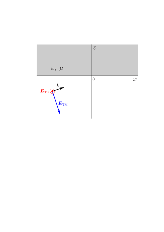
Figure 1: Choice of the coordinate system in the configuration of an electromagnetic wave with a wave vector $\bf{k}$ incident from vacuum on the plane $z=0$ of magnetic medium filling in the semispace $z>0$ (see the text for further discussion).

The Maxwell equations inside the magnetic medium with no external charges and currents take the standard form

$${\rm rot}\mbox{\boldmath$E$}=-\frac{1}{c}\frac{\partial\mbox{\boldmath$B$}}{\partial t},$$ (1)

$${\rm rot}\mbox{\boldmath$H$}=\frac{1}{c}\frac{\partial\mbox{\boldmath$D$}}{\partial t},$$ (2)

$${\rm div}\mbox{\boldmath$B$}=0,\quad{\rm div}\mbox{\boldmath$D$}=0,$$ (3)

where $E$ is the electric field, $B$ is the magnetic induction, $H$ is the magnetic field, and $D$ is the electric displacement. With our choice of the coordinate system, all these fields have the form

$$\mbox{\boldmath$F$}(t,\mbox{\boldmath$r$})=\mbox{\boldmath$F$}(t,\mbox{\boldmath$r$};\omega,k_{x})=\mbox{\boldmath$F$}{(z;\omega,k_{x})}e^{-i\omega t+ik_{x}x}.$$ (4)

Below we briefly repeat a derivation of the exact impedances performed in Ref. 49 for nonmagnetic media making the corresponding generalizations to the magnetic case where necessary. Note that in experiments on measuring the Casimir interaction magnetic metal is nonmagnetized in order to avoid an impact of the additional magnetic force. In doing so our choice $k_{y}=0$ is not restrictive because we consider a homogeneous isotropic medium where the preferential direction is fixed only by the wave vector leading to tensor character of the dielectric properties (see below). As a result, in the end of derivation one can replace $k_{x}$ with $k_{\bot}=(k_{x}^{2}+k_{y}^{2})^{1/2}$.

We start from the derivation of exact surface impedance for the TE polarization of the electromagnetic field which is defined as 48 ; 49 ; 52 ; 55

$$Z_{\rm TE}(\omega,{k_{\bot}})=-\frac{E_{y}(+0;\omega,{k_{\bot}})}{H_{x}(+0;\omega,{k_{\bot}})}.$$ (5)

For the TE-polarized field $\mbox{\boldmath$E$}_{\rm TE}(t,\mbox{\boldmath$r$})=\left(0,E_{y}(t,\mbox{\boldmath$r$}),0\right)$ and from Eq. (1) using Eq. (4) we obtain

$$B_{x}{(z;\omega,k_{x})}=\frac{ic}{\omega}\frac{dE_{y}{(z;\omega,k_{x})}}{dz},$$

$$B_{z}{(z;\omega,k_{x})}=\frac{ck_{x}}{\omega}E_{y}{(z;\omega,k_{x})}.$$ (6)

From this it follows that both equalities in Eq. (3) are satisfied automatically.

Now we consider the respective magnetic field $\mbox{\boldmath$H$}(t,\mbox{\boldmath$r$})=\big{(}H_{x}(t,\mbox{\boldmath$r$}),0,H_{z}(t,\mbox{\boldmath$r$})\big{)}$ and electric displacement $\mbox{\boldmath$D$}_{\rm TE}(t,\mbox{\boldmath$r$})=\big{(}0,D_{y}(t,\mbox{\boldmath$r$}),0\big{)}$. Using Eq. (4), from Eq. (2) one finds

$$\frac{dH_{x}{(z;\omega,k_{x})}}{dz}-ik_{x}H_{z}{(z;\omega,k_{x})}=-\frac{i\omega}{c}D_{y}{(z;\omega,k_{x})}.$$ (7)

Below we assume that the effects of spatial dispersion are important for only dielectric properties of our medium and are unrelated to its magnetic properties. Then for the fields under consideration depending on $t$ as $\exp(-i\omega t)$ it holds

$$B_{x,z}{(z;\omega,k_{x})}=\mu(\omega)H_{x,z}{(z;\omega,k_{x})},$$ (8)

where $\mu(\omega)$ is the frequency-dependent magnetic permeability of a metal filling the semispace $z>0$.

Substituting Eq. (8) in Eq. (7), one obtains

$$\frac{1}{\mu(\omega)}\frac{dB_{x}{(z;\omega,k_{x})}}{dz}-\frac{ik_{x}}{\mu(\omega)}B_{z}{(z;\omega,k_{x})}+\frac{i\omega}{c}D_{y}{(z;\omega,k_{x})}=0.$$ (9)

Taking into account Eq. (6), this equation can be rewritten as

$$\frac{d^{2}E_{y}{(z;\omega,k_{x})}}{dz^{2}}-k_{x}^{2}E_{y}{(z;\omega,k_{x})}+\mu(\omega)\frac{\omega^{2}}{c^{2}}D_{y}{(z;\omega,k_{x})}=0.$$ (10)

The above equations are valid inside a medium, i.e., for $z>0$. In order to take into account the effects of spatial dispersion, one should use the condition of space homogeneity 55 ; 56 . To satisfy this condition, we assume that our medium fills in not a semispace, as in Fig. 1, but all of space $-\infty<z<\infty$. In so doing it is assumed that electrons are reflected specularly on the plane $z=0$, i.e., the following conditions are satisfied 49 :

$$E_{x,y}{(z;\omega,k_{x})}=E_{x,y}(-z;\omega,k_{x}),$$

$$E_{z}{(z;\omega,k_{x})}=-E_{z}(-z;\omega,k_{x}),$$

$$D_{x,y}{(z;\omega,k_{x})}=D_{x,y}(-z;\omega,k_{x}),$$

$$D_{z}{(z;\omega,k_{x})}=-D_{z}(-z;\omega,k_{x}).$$ (11)

Under these conditions one can perform the Fourier transform of all fields along the $z$-axis defined as

$$\widetilde{\mbox{\boldmath$F$}}{(\omega,k_{x},k_{z})}=\int_{-\infty}^{\infty}\!\!dz\mbox{\boldmath$F$}{(z;\omega,k_{x})}e^{-ik_{z}z}$$ (12)

and the inverse Fourier transform

$${\mbox{\boldmath$F$}}{(z;\omega,k_{x})}=\frac{1}{2\pi}\int_{-\infty}^{\infty}\!\!dk_{z}\widetilde{\mbox{\boldmath$F$}}{(\omega,k_{x},k_{z})}e^{ik_{z}z}.$$ (13)

Calculating the Fourier transform of both sides of Eq. (10), one obtains

$$I{(\omega,k_{x},k_{z})}-k_{x}^{2}\widetilde{E}_{y}{(\omega,k_{x},k_{z})}+\mu(\omega)\frac{\omega^{2}}{c^{2}}\widetilde{D}_{y}{(\omega,k_{x},k_{z})}=0,$$ (14)

where the following notation is introduced

$$I{(\omega,k_{x},k_{z})}\equiv\int_{-\infty}^{\infty}\!\!dz\frac{d^{2}E_{y}{(z;\omega,k_{x})}}{dz^{2}}e^{-ik_{z}z}$$

$$~{}~{}~{}=\int_{0}^{\infty}\!d\left(\frac{dE_{y}{(z;\omega,k_{x})}}{dz}\right)e^{-ik_{z}z}$$ (15)

$$~{}~{}~{}~{}~{}~{}~{}~{}~{}~{}~{}~{}~{}~{}~{}+\int_{-\infty}^{0}\!d\left(\frac{dE_{y}{(z;\omega,k_{x})}}{dz}\right)e^{-ik_{z}z}.$$

Integrating on the right-hand side of Eq. (15) by parts for two times with account of Eqs. (11) and (12), we find

$$I{(\omega,k_{x},k_{z})}=-k_{z}^{2}\widetilde{E}_{y}{(\omega,k_{x},k_{z})}-2\frac{dE_{y}(+0;\omega,k_{x})}{dz},$$ (16)

where the last term on the right-hand side originates from a discontinuity of the derivative $dE_{y}{(z;\omega,k_{x})}/dz$ at $z=0$.

Substituting Eq. (16) in Eq. (14), one obtains

$$-(k_{x}^{2}+k_{z}^{2})\widetilde{E}_{y}{(\omega,k_{x},k_{z})}+\mu(\omega)\frac{\omega^{2}}{c^{2}}\widetilde{D}_{y}{(\omega,k_{x},k_{z})}$$

$$~{}~{}~{}~{}~{}~{}~{}~{}~{}~{}~{}~{}~{}~{}~{}~{}~{}~{}~{}~{}=2\frac{dE_{y}(+0;\omega,k_{x})}{dz}.$$ (17)

On the other hand, from the first equality in Eq. (6) and Eq. (8) taken at $z=+0$ we arrive at

$$\frac{dE_{y}(+0;\omega,k_{x})}{dz}=-i\mu(\omega)\frac{\omega}{c}H_{x}(+0;\omega,k_{x}).$$ (18)

Taking into account that we deal with the TE polarization, $\mbox{\boldmath$E$}_{\rm TE}\bot\mbox{\boldmath$k$}$, it holds 55 ; 56

$$\widetilde{D}_{y}{(\omega,k_{x},k_{z})}={\varepsilon^{\rm Tr}}(\omega,{\mbox{\boldmath$k$}})\widetilde{E}_{y}{(\omega,k_{x},k_{z})},$$ (19)

where ${\varepsilon^{\rm Tr}}(\omega,{\mbox{\boldmath$k$}})$ is the transverse dielectric permittivity.

Substituting Eqs. (18) and (19) in Eq. (17), one finds

$$\frac{\widetilde{E}_{y}{(\omega,k_{x},k_{z})}}{H_{x}(+0;\omega,k_{x})}=-2i\frac{\mu(\omega){\omega}{c}}{\mu(\omega){\varepsilon^{\rm Tr}}(\omega,{\mbox{\boldmath$k$}}){\omega^{2}}-c^{2}(k_{x}^{2}+k_{z}^{2})}.$$ (20)

For any choice of the coordinate system in the $z=0$ plane one should replace $k_{x}$ with ${k_{\bot}}$ in Eq. (20). After this replacement, we make the inverse Fourier transform (13) on both sides of Eq. (20) and putting $z=+0$ obtain the final result for the TE surface impedance defined in Eq. (5)

$$Z_{\rm TE}(\omega,{k_{\bot}})=i\frac{\mu(\omega){\omega}{c}}{\pi}\int_{-\infty}^{\infty}\frac{dk_{z}}{\mu(\omega){\varepsilon^{\rm Tr}}(\omega,{\mbox{\boldmath$k$}}){\omega^{2}}-c^{2}{\mbox{\boldmath$k$}}^{2}},$$ (21)

where ${\mbox{\boldmath$k$}}^{2}={k_{\bot}^{2}}+k_{z}^{2}$. For a nonmagnetic medium, $\mu(\omega)=1$, the result (21) coincides with that obtained in Refs. 48 ; 49 .

We are coming now to the derivation of exact surface impedance for the TM polarization of the electromagnetic field which is defined as 48 ; 49 ; 52 ; 55

$$Z_{\rm TM}(\omega,{k_{\bot}})=\frac{E_{x}(+0;\omega,{k_{\bot}})}{H_{y}(+0;\omega,{k_{\bot}})}.$$ (22)

The TM polarized field $\mbox{\boldmath$E$}_{\rm TM}(t,{\mbox{\boldmath$r$}})=\left(E_{x}(t,{\mbox{\boldmath$r$}}),0,E_{z}(t,{\mbox{\boldmath$r$}})\right)$ has two nonzero components (see Fig. 1). This makes the case of TM polarization more complicated. Taking into account that all field components are given by Eq. (4), one finds $\mbox{\boldmath$B$}_{\rm TM}(t,{\mbox{\boldmath$r$}})=\left(0,B_{y}(t,{\mbox{\boldmath$r$}}),0\right)$ and Eq. (1) takes the form

$$\frac{dE_{x}{(z;\omega,k_{x})}}{dz}-ik_{x}E_{z}{(z;\omega,k_{x})}=\frac{i\omega}{c}B_{y}{(z;\omega,k_{x})}.$$ (23)

In a similar way, we have $\mbox{\boldmath$H$}_{\rm TM}(t,{\mbox{\boldmath$r$}})=\left(0,H_{y}(t,{\mbox{\boldmath$r$}}),0\right)$ and $\mbox{\boldmath$D$}_{\rm TM}(t,{\mbox{\boldmath$r$}})=\left(D_{x}(t,{\mbox{\boldmath$r$}}),0,D_{z}(t,{\mbox{\boldmath$r$}})\right)$ where all components are given by Eq. (4). As a result, Eq. (2) leads to

$$\frac{dH_{y}{(z;\omega,k_{x})}}{dz}=\frac{i\omega}{c}D_{x}{(z;\omega,k_{x})},$$

$$k_{x}H_{y}{(z;\omega,k_{x})}=-\frac{\omega}{c}D_{z}{(z;\omega,k_{x})}.$$ (24)

Taking into account that, in addition to Eq. (8), it also holds

$$B_{y}{(z;\omega,k_{x})}=\mu(\omega)H_{y}{(z;\omega,k_{x})},$$ (25)

we bring Eq. (24) to the form

$$\frac{dB_{y}{(z;\omega,k_{x})}}{dz}-i\mu(\omega)\frac{\omega}{c}D_{x}{(z;\omega,k_{x})}=0,$$

$$k_{x}B_{y}{(z;\omega,k_{x})}+\mu(\omega)\frac{\omega}{c}D_{z}{(z;\omega,k_{x})}=0.$$ (26)

We express $B_{y}{(z;\omega,k_{x})}$ from the second equality in Eq. (26) and substitute to the right-hand side of Eq. (23). The result is

$$ik_{x}\frac{dE_{x}{(z;\omega,k_{x})}}{dz}+k_{x}^{2}E_{z}{(z;\omega,k_{x})}-\mu(\omega)\frac{\omega^{2}}{c^{2}}D_{z}{(z;\omega,k_{x})}=0.$$ (27)

Now we differentiate both sides of Eq. (23) with respect to $z$ and, using the first equality in Eq. (26), obtain

$$\frac{d^{2}E_{x}{(z;\omega,k_{x})}}{dz^{2}}-ik_{x}\frac{\partial E_{z}{(z;\omega,k_{x})}}{\partial z}+\mu(\omega)\frac{\omega^{2}}{c^{2}}D_{x}{(z;\omega,k_{x})}=0.$$ (28)

The Fourier transform of Eq. (27) with account of Eq. (11) leads to

$$k_{x}k_{z}\widetilde{E}_{x}{(\omega,k_{x},k_{z})}-k_{x}^{2}\widetilde{E}_{z}{(\omega,k_{x},k_{z})}$$

$$~{}~{}~{}~{}~{}~{}~{}~{}~{}~{}~{}~{}~{}~{}~{}+\mu(\omega)\frac{\omega^{2}}{c^{2}}\widetilde{D}_{z}{(\omega,k_{x},k_{z})}=0.$$ (29)

The Fourier transform of Eq. (28) can be written in the form

$$I_{1}{(\omega,k_{x},k_{z})}-ik_{x}I_{2}{(\omega,k_{x},k_{z})}+\mu(\omega)\frac{\omega^{2}}{c^{2}}\widetilde{D}_{x}{(\omega,k_{x},k_{z})}=0,$$ (30)

where the integrals

$$I_{1}{(\omega,k_{x},k_{z})}\equiv\int_{-\infty}^{\infty}\frac{d^{2}E_{x}{(z;\omega,k_{x})}}{dz^{2}}e^{-ik_{z}z}dz,$$

$$I_{2}{(\omega,k_{x},k_{z})}\equiv\int_{-\infty}^{\infty}\frac{\partial E_{z}{(z;\omega,k_{x})}}{\partial z}e^{-ik_{z}z}dz$$ (31)

are calculated similar to Eqs. (15) and (16) under conditions (11) with the results

$$I_{1}{(\omega,k_{x},k_{z})}=-2\frac{dE_{x}(+0;\omega,k_{x})}{dz}-k_{z}^{2}\widetilde{E}_{x}{(\omega,k_{x},k_{z})},$$

(32)

$$I_{2}{(\omega,k_{x},k_{z})}=-2E_{z}(+0;\omega,k_{x})+ik_{z}\widetilde{E}_{z}{(\omega,k_{x},k_{z})}.$$

The additional terms on the right-hand side of these equalities originate from the discontinuities of the quantities $dE_{x}{(z;\omega,k_{x})}/dz$ and $E_{z}{(z;\omega,k_{x})}$ at $z=0$.

Substituting Eq. (32) in Eq. (30), we obtain

$$-k_{z}^{2}\widetilde{E}_{x}{(\omega,k_{x},k_{z})}+k_{x}k_{z}\widetilde{E}_{z}{(\omega,k_{x},k_{z})}$$

$$~{}~{}~{}~{}~{}~{}~{}~{}~{}+\mu(\omega)\frac{\omega^{2}}{c^{2}}\widetilde{D}_{x}{(\omega,k_{x},k_{z})}$$ (33)

$$~{}~{}~{}~{}~{}~{}~{}~{}~{}=2\frac{dE_{x}(+0;\omega,k_{x})}{dz}-2ik_{x}E_{z}(+0;\omega,k_{x}).$$

With account of Eq. (25), the first Maxwell equation (23) taken at $z=+0$ is

$$\frac{dE_{x}(+0;\omega,k_{x})}{dz}-ik_{x}E_{z}(+0;\omega,k_{x})=i\mu(\omega)\frac{\omega}{c}H_{y}(+0;\omega,k_{x}).$$ (34)

Substituting this in Eq. (33), one obtains

$$-k_{z}^{2}\widetilde{E}_{x}{(\omega,k_{x},k_{z})}+k_{x}k_{z}\widetilde{E}_{z}{(\omega,k_{x},k_{z})}$$ (35)

$$~{}~{}+\mu(\omega)\frac{\omega^{2}}{c^{2}}\widetilde{D}_{x}{(\omega,k_{x},k_{z})}=2i\mu(\omega)\frac{\omega}{c}H_{y}(+0;\omega,k_{x}).$$

Equations (29) and (35) taken together give the possibility to find the surface impedance $Z_{\rm TM}$ defined in Eq. (22). In the presence of spatial dispersion, the quantities $\widetilde{D}_{x}{(\omega,k_{x},k_{z})}$ and $\widetilde{D}_{z}{(\omega,k_{x},k_{z})}$ are the linear combinations of $\widetilde{E}_{x}{(\omega,k_{x},k_{z})}$ and $\widetilde{E}_{z}{(\omega,k_{x},k_{z})}$ where the components of the dielectric tensor serve as the coefficients 55 ; 56

$$\widetilde{D}_{x}{(\omega,k_{x},k_{z})}={\varepsilon}_{xx}\widetilde{E}_{x}{(\omega,k_{x},k_{z})}+{\varepsilon}_{xz}\widetilde{E}_{z}{(\omega,k_{x},k_{z})},$$

(36)

$$\widetilde{D}_{z}{(\omega,k_{x},k_{z})}={\varepsilon}_{zx}\widetilde{E}_{x}{(\omega,k_{x},k_{z})}+{\varepsilon}_{zz}\widetilde{E}_{z}{(\omega,k_{x},k_{z})}.$$

In Ref. 49 the tensor ${\varepsilon}_{ij}$ was diagonalized by rotating the coordinate system $(x,z)$ about $y$ axis by the angle $\varphi$ such that $\sin\varphi=k_{x}/k$, $\cos\varphi=k_{z}/k$. In the rotated coordinates $(x^{\prime},z^{\prime})$ the wave vector $k$ is directed along the $z^{\prime}$-axis and the dielectric tensor takes a diagonal form with the components ${\varepsilon^{\rm Tr}}$ and ${\varepsilon^{\,\rm L}}$ where ${\varepsilon^{\,\rm L}}$ is the longitudinal dielectric permittivity (we omit for brevity the arguments $\omega$ and $k$ in components of the dielectric tensor).

In Ref. 49 it was shown that

$${\varepsilon}_{xx}=\frac{1}{k_{x}^{2}+k_{z}^{2}}\left({\varepsilon^{\rm Tr}}k_{z}^{2}+{\varepsilon^{\,\rm L}}k_{x}^{2}\right),$$

$${\varepsilon}_{zz}=\frac{1}{k_{x}^{2}+k_{z}^{2}}\left({\varepsilon^{\rm Tr}}k_{x}^{2}+{\varepsilon^{\,\rm L}}k_{z}^{2}\right),$$

$${\varepsilon}_{xz}={\varepsilon}_{zx}=\left({\varepsilon^{\,\rm L}}-{\varepsilon^{\rm Tr}}\right)\frac{k_{x}k_{z}}{k_{x}^{2}+k_{z}^{2}}.$$ (37)

With account of (36), we rewrite Eqs. (29) and (35) in the following equivalent form:

$$\Big{[}k_{x}k_{z}+\mu(\omega)\frac{\omega^{2}}{c^{2}}{\varepsilon}_{zx}\Big{]}\widetilde{E}_{x}{(\omega,k_{x},k_{z})}+\Big{[}-k_{x}^{2}+\mu(\omega)\frac{\omega^{2}}{c^{2}}{\varepsilon}_{zz}\Big{]}\widetilde{E}_{z}{(\omega,k_{x},k_{z})}=0,$$ (38)

$$\Big{[}-k_{z}^{2}+\mu(\omega)\frac{\omega^{2}}{c^{2}}{\varepsilon}_{xx}\Big{]}\widetilde{E}_{x}{(\omega,k_{x},k_{z})}+\Big{[}k_{x}k_{z}+\mu(\omega)\frac{\omega^{2}}{c^{2}}{\varepsilon}_{xz}\Big{]}\widetilde{E}_{z}{(\omega,k_{x},k_{z})}=2i\mu(\omega)\frac{\omega}{c}H_{y}(+0;\omega,k_{x}).$$

By solving this system of linear equations with respect to $\widetilde{E}_{x}{(\omega,k_{x},k_{z})}$ and using Eq. (37) for the components of a nondiagonal dielectric tensor, we obtain

$$\frac{\widetilde{E}_{x}{(\omega,k_{x},k_{z})}}{H_{y}(+0;\omega,k_{x})}=2i\frac{c\omega\mu(\omega)}{k_{x}^{2}+k_{z}^{2}}$$ (39)

$$\times\left[\frac{k_{x}^{2}}{\mu(\omega)\omega^{2}{\varepsilon^{\,\rm L}}(\omega,{\mbox{\boldmath$k$}})}+\frac{k_{z}^{2}}{\mu(\omega)\omega^{2}{\varepsilon^{\rm Tr}}(\omega,{\mbox{\boldmath$k$}})-c^{2}(k_{x}^{2}+k_{z}^{2})}\right].$$

By replacing here $k_{x}$ with ${k_{\bot}}$, as was already done in the case of the TE polarization, and performing the inverse Fourier transform, we find the TM surface impedance (22) for a magnetic medium

$$Z_{\rm TM}(\omega,{k_{\bot}})=i\frac{c\omega\mu(\omega)}{\pi}\int_{-\infty}^{\infty}\frac{dk_{z}}{{\mbox{\boldmath$k$}}^{2}}\left[\frac{{k_{\bot}^{2}}}{\mu(\omega)\omega^{2}{\varepsilon^{\,\rm L}}(\omega,{\mbox{\boldmath$k$}})}\right.$$

$$~{}~{}~{}~{}~{}~{}\left.+\frac{k_{z}^{2}}{\mu(\omega)\omega^{2}{\varepsilon^{\rm Tr}}(\omega,{\mbox{\boldmath$k$}})-c^{2}{\mbox{\boldmath$k$}}^{2}}\right].$$ (40)

For a nonmagnetic medium, this result coincides with respective results of Refs. 48 ; 49 .

For calculation of the Casimir interaction in the framework of the Lifshitz theory (see the next section), one needs the values of surface impedances at the pure imaginary Matsubara frequencies $i\xi_{l}$, where $\xi_{l}=2\pi k_{B}Tl/\hbar$, $k_{B}$ is the Boltzmann constant, $T$ is the temperature, and $l=0,\,1,\,2,\,\ldots$ is an integer number. Substituting $\omega=i\xi_{l}$ in Eqs. (21) and (40), one obtains

$$Z_{\rm TE}(i\xi_{l},{k_{\bot}})=\frac{c\xi_{l}\mu_{l}}{\pi}\int_{-\infty}^{\infty}\frac{dk_{z}}{\mu_{l}{\varepsilon_{l}^{\rm Tr}}({\mbox{\boldmath$k$}}){\xi_{l}^{2}}+c^{2}{\mbox{\boldmath$k$}}^{2}},$$

$$Z_{\rm TM}(i\xi_{l},{k_{\bot}})=\frac{c\xi_{l}\mu_{l}}{\pi}\int_{-\infty}^{\infty}\frac{dk_{z}}{{\mbox{\boldmath$k$}}^{2}}\left[\frac{{k_{\bot}^{2}}}{\mu_{l}\xi_{l}^{2}{\varepsilon_{l}^{\,\rm L}}({\mbox{\boldmath$k$}})}\right.$$

$$~{}~{}~{}~{}~{}~{}\left.+\frac{k_{z}^{2}}{\mu_{l}\xi_{l}^{2}{\varepsilon_{l}^{\rm Tr}}({\mbox{\boldmath$k$}})+c^{2}{\mbox{\boldmath$k$}}^{2}}\right],$$ (41)

where ${\varepsilon_{l}^{\rm Tr}}({\mbox{\boldmath$k$}})\equiv{\varepsilon^{\rm Tr}}(i\xi_{l},{\mbox{\boldmath$k$}})$, ${\varepsilon_{l}^{\,\rm L}}({\mbox{\boldmath$k$}})\equiv{\varepsilon^{\,\rm L}}(i\xi_{l},{\mbox{\boldmath$k$}})$, and $\mu_{l}\equiv\mu(i\xi_{l})$.

In terms of the surface impedances (41) the amplitude reflection coefficients on the boundary plane of magnetic metal for two polarizations of the electromagnetic field take the form 48 ; 49 ; 55

$$r_{\rm TM}{(i\xi_{l},k_{\bot})}=\frac{cq_{l}-\xi_{l}Z_{\rm TM}{(i\xi_{l},k_{\bot})}}{cq_{l}+\xi_{l}Z_{\rm TM}{(i\xi_{l},k_{\bot})}},$$

$$r_{\rm TE}{(i\xi_{l},k_{\bot})}=\frac{cq_{l}Z_{\rm TE}{(i\xi_{l},k_{\bot})}-\xi_{l}}{cq_{l}Z_{\rm TE}{(i\xi_{l},k_{\bot})}+\xi_{l}},$$ (42)

where $q_{l}\equiv{({k_{\bot}^{2}}+\xi_{l}^{2}/c^{2})^{1/2}}$.

Equations (41) and (42) make it possible to apply the Lifshitz theory to the case of magnetic metal boundary plates possessing spatially nonlocal dielectric response.

III The Casimir pressure between magnetic metal plates described by the alternative nonlocal response functions

As was mentioned in Sec. I, the Lifshitz formula for the Casimir pressure $P$ between two parallel plates (semispaces) spaced at a distance $a$ was derived within the quantum-field-theoretical and statistical approaches. In terms of reflection coefficients on the boundary surfaces it can be written as 13 ; 22 ; 23

$$P(a,T)=-\frac{k_{B}T}{\pi}\sum_{l=0}^{\infty}{\vphantom{\sum}}^{\prime}\int_{0}^{\infty}\!\!\!q_{l}{k_{\bot}}d{k_{\bot}}$$

$$~{}~{}~{}~{}~{}~{}~{}~{}~{}~{}~{}~{}~{}~{}~{}\times\sum_{\alpha}\left[r_{\alpha}^{-2}{(i\xi_{l},k_{\bot})}e^{2aq_{l}}-1\right]^{-1}\!\!,$$ (43)

where the prime on the summation sign in $l$ divides the term with $l=0$ by 2 and the sum in $\alpha$ is over two polarizations of the electromagnetic field, $\alpha={\rm TM}$ and $\alpha={\rm TE}$. For magnetic plates demonstrating a spatially nonlocal dielectric response the reflection coefficients entering Eq. (43) are given by Eqs. (41) and (42). Note that the Casimir pressure between metallic plates of more than 100 nm thickness can be already considered as between semispaces and calculated using Eq. (43) 13 .

We consider the Casimir pressure between two parallel plates made of magnetic metal Ni which is not magnetized, so that there is no magnetic force in addition to the Casimir one. The dielectric response of Ni is supposed to be spatially nonlocal and described by the alternative response functions introduced in Ref. 53

$${\varepsilon^{\rm Tr}}(\omega,{k_{\bot}})=1-\frac{\omega_{p}^{2}}{\omega(\omega+i\gamma)}\left(1+i\frac{{v^{\rm Tr}}{k_{\bot}}}{\omega}\right),$$

$${\varepsilon^{\,\rm L}}(\omega,{k_{\bot}})=1-\frac{\omega_{p}^{2}}{\omega(\omega+i\gamma)}\left(1+i\frac{{v^{\,\rm L}}{k_{\bot}}}{\omega}\right)^{-1}\!\!\!.$$ (44)

Here, $\omega_{p}$ is the plasma frequency and $\gamma$ is the relaxation parameter (the latter depends on $T$), and ${v^{\rm Tr}}$, ${v^{\,\rm L}}$ are the constants of the order of Fermi velocity $v_{F}\sim 0.01c$.

The distinctive feature of response functions (44) is that they nearly coincide with the standard local Drude response function

$${\varepsilon}^{D}(\omega)=1-\frac{\omega_{p}^{2}}{\omega(\omega+i\gamma)}$$ (45)

for the electromagnetic fields on the mass shell. This is because

$$\frac{v^{\rm Tr,L}{k_{\bot}}}{\omega}\sim\frac{v_{F}}{c}\,\frac{c{k_{\bot}}}{\omega}\leqslant\frac{v_{F}}{c}\ll 1.$$ (46)

As a consequence, the alternative response functions (44) leads to almost the same results, as the Drude function (45), for the on-shell fields. This is not the case, however, for the off-shell electromagnetic fields for which the parameter (46) can be large.

Although the response functions (44) are of phenomenological character, they take dissipation into account and simultaneously satisfy the Kramers-Kronig relations and lead to an agreement of the Lifshitz theory with experiments on measuring the Casimir interaction between Au surfaces 53 . According to the results of Ref. 54 , the Casimir entropy calculated using Eq. (44) satisfies the Nernst heat theorem. Thus, it is of prime importance to test the alternative response functions (44) in the case of magnetic media.

For the response functions ${\varepsilon_{l}^{\rm Tr}}$ and ${\varepsilon_{l}^{\,\rm L}}$ depending only on ${k_{\bot}}$, the integrals in Eq. (41) are easily calculated

$$Z_{\rm TE}{(i\xi_{l},k_{\bot})}=\frac{\xi_{l}\mu_{l}}{\sqrt{c^{2}{k_{\bot}^{2}}+\mu_{l}{\varepsilon_{l}^{\rm Tr}}({k_{\bot}})\xi_{l}^{2}}},$$ (47)

$$Z_{\rm TM}{(i\xi_{l},k_{\bot})}=\frac{1}{\xi_{l}}\left[\vphantom{\frac{\sqrt{\mu_{l}{\varepsilon_{l}^{\rm Tr}}({k_{\bot}})\xi_{l}^{2}}}{{\varepsilon_{l}^{\rm Tr}}({k_{\bot}})}}\frac{c{k_{\bot}}}{{\varepsilon_{l}^{\,\rm L}}({k_{\bot}})}\right.$$

$$~{}~{}~{}~{}~{}~{}~{}~{}~{}~{}~{}~{}~{}~{}~{}\left.+\frac{\sqrt{c^{2}{k_{\bot}^{2}}+\mu_{l}{\varepsilon_{l}^{\rm Tr}}({k_{\bot}})\xi_{l}^{2}}-c{k_{\bot}}}{{\varepsilon_{l}^{\rm Tr}}({k_{\bot}})}\right].$$

Substituting Eq. (47) in Eq. (42), one arrives at

$$r_{\rm TM}{(i\xi_{l},k_{\bot})}=\frac{q_{l}{\varepsilon_{l}^{\rm Tr}}({k_{\bot}})-k_{\mu}^{\rm Tr}{(i\xi_{l},k_{\bot})}-{k_{\bot}}[{\varepsilon_{l}^{\rm Tr}}({k_{\bot}})-{\varepsilon_{l}^{\,\rm L}}({k_{\bot}})][{\varepsilon_{l}^{\,\rm L}}({k_{\bot}})]^{-1}}{q_{l}{\varepsilon_{l}^{\rm Tr}}({k_{\bot}})+k_{\mu}^{\rm Tr}{(i\xi_{l},k_{\bot})}+{k_{\bot}}[{\varepsilon_{l}^{\rm Tr}}({k_{\bot}})-{\varepsilon_{l}^{\,\rm L}}({k_{\bot}})][{\varepsilon_{l}^{\,\rm L}}({k_{\bot}})]^{-1}},$$

$$r_{\rm TE}{(i\xi_{l},k_{\bot})}=\frac{q_{l}\mu_{l}-k_{\mu}^{\rm Tr}{(i\xi_{l},k_{\bot})}}{q_{l}\mu_{l}+k_{\mu}^{\rm Tr}{(i\xi_{l},k_{\bot})}},$$ (48)

where

$$k_{\mu}^{\rm Tr}{(i\xi_{l},k_{\bot})}=\left[{k_{\bot}^{2}}+\mu_{l}{\varepsilon_{l}^{\rm Tr}}({k_{\bot}})\frac{\xi_{l}^{2}}{c^{2}}\right]^{1/2}$$ (49)

and ${\varepsilon_{l}^{\rm Tr}}$, ${\varepsilon_{l}^{\,\rm L}}$ are given by Eq. (44) where one should put $\omega=i\xi_{l}$.

Numerical computations of the Casimir pressure were performed by using Eqs. (43), (44), and (48) at $T=300~{}$K. For Ni we have used the following values of all parameters: $\hbar\omega_{p}=4.89~{}$eV, $\hbar\gamma=0.0436~{}$eV 57 ; 58 , $\mu_{0}=110$ at $T=300~{}$K 32 ; 33 ; 59 , $v_{F}=1.31\times 10^{6}~{}$m/s determined in the approximation of a spherical Fermi surface, and ${v^{\rm Tr}}={v^{\,\rm L}}=7v_{F}$ as was used in Ref. 53 for the best agreement between experiment and theory for Au test bodies (similar to Ref. 53 the below results are nearly independent on the value of ${v^{\,\rm L}}$ in the region $0\leqslant{v^{\,\rm L}}\leqslant 10v_{F}$).

It should be noted that the magnetic permeability $\mu(i\xi_{l})$ quickly decreases with $l$ and becomes equal to unity at frequencies much below the first Matsubara frequency. Because of this, magnetic properties influence the Casimir interaction only through the zero-frequency term of the Lifshitz formula (43) 60 . In the contribution of all terms with $l\geqslant 1$, one should put $\mu(i\xi_{l})=1$. It is helpful also that at $\xi_{0}=0$ the reflection coefficients (48) take an especially simple form

$$r_{\rm TM}(0,{k_{\bot}})=\frac{\omega_{p}^{2}}{2{v^{\,\rm L}}\gamma{k_{\bot}}+\omega_{p}^{2}},$$ (50)

$$r_{\rm TE}(0,{k_{\bot}})=\frac{\mu_{0}\sqrt{{k_{\bot}}}-\sqrt{{k_{\bot}}+B}}{\mu_{0}\sqrt{{k_{\bot}}}+\sqrt{{k_{\bot}}+B}},$$

where $B\equiv\mu_{0}\omega_{p}^{2}{v^{\rm Tr}}/(\gamma c^{2})$. Interestingly, the magnetic properties make an impact only on the TE polarization.

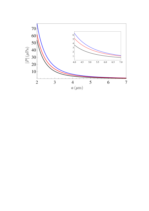
Figure 2: Magnitudes of the Casimir pressure between two parallel magnetic metal plates computed using the alternative nonlocal, plasma, and Drude response functions are shown as functions of separation by the bottom, medium, and top lines, respectively. The region of larger separations is shown in the inset on an enlarged scale.

The computational results for the magnitude of the Casimir pressure are shown in Fig. 2 by the bottom line as a function of separation in the region from 2 to $7~{}\mu$m. It is interesting to compare them with similar results obtained using the standard, spatially local, response functions. In this case we have

$${\varepsilon_{l}^{\,\rm L}}({\mbox{\boldmath$k$}})={\varepsilon_{l}^{\rm Tr}}({\mbox{\boldmath$k$}})={\varepsilon}_{l}={\varepsilon}(i\xi_{l}),$$ (51)

and Eq. (41) simplifies to

$$Z_{\rm TE}{(i\xi_{l},k_{\bot})}=\frac{\xi_{l}\mu_{l}}{\sqrt{c^{2}{k_{\bot}^{2}}+\mu_{l}{\varepsilon}_{l}\xi_{l}^{2}}},$$

$$Z_{\rm TM}{(i\xi_{l},k_{\bot})}=\frac{\sqrt{c^{2}{k_{\bot}^{2}}+\mu_{l}{\varepsilon}_{l}\xi_{l}^{2}}}{\xi_{l}{\varepsilon}_{l}}.$$ (52)

For $\mu_{l}=1$ these impedances were considered in Ref. 61 where it was shown that they lead to the standard Fresnel reflection coefficients. In fact a substitution of Eq. (52) in Eq. (42) results in

$$r_{\rm TM}{(i\xi_{l},k_{\bot})}=\frac{q_{l}{\varepsilon}_{l}-k_{\mu}{(i\xi_{l},k_{\bot})}}{q_{l}{\varepsilon}_{l}+k_{\mu}{(i\xi_{l},k_{\bot})}},$$

$$r_{\rm TE}{(i\xi_{l},k_{\bot})}=\frac{q_{l}\mu_{l}-k_{\mu}{(i\xi_{l},k_{\bot})}}{q_{l}\mu_{l}+k_{\mu}{(i\xi_{l},k_{\bot})}},$$ (53)

where $k_{\mu}{(i\xi_{l},k_{\bot})}$ is obtained from $k_{\mu}^{\rm Tr}{(i\xi_{l},k_{\bot})}$ defined in Eq. (49) by replacing of ${\varepsilon_{l}^{\rm Tr}}$ with ${\varepsilon}_{l}$ according to Eq. (51). Equation (53) presents the standard Fresnel coefficients commonly used in the Lifshitz theory for both nonmagnetic ($\mu_{l}=1$) and magnetic plate materials.

For comparison purposes, we also compute the Casimir pressure (43) between Ni plates using the Fresnel coefficients (53) and local dielectric responses given by the dissipative Drude (45) and dissipationless plasma response functions. At the pure imaginary Matsubara frequencies these functions are given by

$${\varepsilon}_{l}^{D}=1+\frac{\omega_{p}^{2}}{\xi_{l}(\xi_{l}+\gamma)},\qquad{\varepsilon}_{l}^{p}=1+\frac{\omega_{p}^{2}}{\xi_{l}^{2}}.$$ (54)

The computational results as the functions of separation are presented in Fig. 2 by the top and middle lines, respectively. In an inset, the region of larger separations is shown on an enlarged scale. As is seen in Fig. 2, the alternative nonlocal response functions (bottom line) lead to markedly smaller theoretical values of the pressure magnitude $|P_{nl}|$ than $|P_{p}|$ computed using the plasma function (middle line) and $|P_{D}|$ computed using the Drude response function over the entire range of separations from 2 to $7~{}\mu$m. As an example, at $a=4~{}\mu$m one has $P_{nl}/P_{p}\approx 0.70$ and $P_{nl}/P_{D}\approx 0.57$. At $a=6~{}\mu$m the same ratios are equal to $P_{nl}/P_{p}\approx 0.66$ and $P_{nl}/P_{D}\approx 0.57$.

In order to perform a comparison between the three response functions over a wider range of separations, in Fig. 3 we plot the ratios of $P_{nl}$ and $P_{p}$ to $P_{D}$. In so doing, we have taken into account that at separations below approximately $1~{}\mu$m the response functions are influenced by the interband transitions of electrons. An impact of these transitions becomes larger when the separation decreases. It is included in the response functions due to conduction electrons considered above by replacing the unities after the signs of equality on the right-hand sides of Eqs. (44) and (54) with the appropriate function of $\xi_{l}$ found by means of the Kramers-Kronig relations from the measured optical data of Ni 57 (see Refs. 13 ; 33 for details).

                          

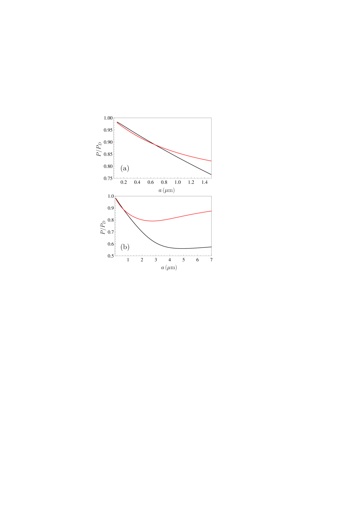
Figure 3: Ratios of the Casimir pressure between two parallel magnetic metal plates computed using the alternative nonlocal and plasma response functions to the same pressure computed using the Drude response function ($P_{nl}/P_{D}$ and $P_{p}/P_{D}$, respectively) are shown by the two lines over the separation regions (a) from 100 nm to $1.5~{}\mu$m and (b) from 100 nm to $7~{}\mu$m. In the region from from 100 to 655 nm the upper lines are for $P_{nl}/P_{D}$ and the lower lines are for $P_{p}/P_{D}$, and quite the reverse in the region from 655 nm to $7~{}\mu$m.

In Fig. 3(a) the ratios $P_{p}/P_{D}$ and $P_{nl}/P_{D}$ are shown as functions of separation by the lower and upper lines in the region from 100 to 655 nm, respectively. At $a\approx 655~{}$nm the lines cross each other. At larger separations the ratio $P_{p}/P_{D}$ is given by the upper line and the ratio $P_{nl}/P_{D}$ — by the lower one. In Fig. 3(b) these lines are shown over the entire range of separations from 100 nm to $7~{}\mu$m. Note that at separations below 100 nm theoretical predictions using all three response functions nearly coincide.

As is seen in Fig. 3(a), within the separation region from 100 to 800 nm the Casimir pressure between magnetic metal plates computed using the alternative nonlocal and local plasma response functions differ by less than 1%. This should be compared with the fact that almost equal Casimir pressures predicted by these response functions differ from that predicted by the Drude function by 2% at $a=100~{}$nm at by 13% already at $a=800~{}$nm. According to Fig. 3(b), at separations of a few micrometers the Casimir pressures predicted by the Lifshitz theory using all three response functions differ widely. With further increase of separation the Casimir pressure calculated using the alternative nonlocal and plasma response functions approach each other and the classical limit reached in the case of plates described by the Drude function and made of an ideal metal. This, however, holds at separations of the order of millimeters which are immaterial due to negligibly small force values.

In the next section, we compare the theoretical predictions obtained using both local and nonlocal response functions with the measurement data.

IV Comparison between experiment and theory

Experiments of Refs. 32 ; 33 are devoted to measurements of the Casimir interaction in the configuration of a Ni-coated hollow glass sphere with $R=61.71~{}\mu$m radius and a Ni-coated Si plate. The Ni coatings on both bodies were sufficiently thick in order they could be treated as all-nickel when considering the Casimir interaction. These experiments were performed in high vacuum at $T=300~{}$K by using the dynamic atomic force microscope based setup operated in the frequency-shift mode. Because of this, an immediately measured quantity was the gradient of the Casimir force between a sphere and a plate $F_{sp}^{\prime}(a,T)=\partial F_{sp}(a,T)/\partial a$.

According to the proximity force approximation, which is very accurate under the condition $a\ll R$ (see below), the gradient of the Casimir force in a sphere-plate geometry is expressed via the Casimir pressure between two parallel plates as 11 ; 13

$$F_{sp}^{\prime}(a,T)=-2\pi RP(a,T).$$ (55)

This gives the possibility to compare the measurement results with theoretical predictions of the Lifshitz theory for the Casimir pressure considered in Sec. III.

To perform a comparison between experiment and theory, one should take into account very small corrections to the result (55) arising due to the surface roughness on metallic coatings of a sphere and a plate 11 ; 13 ; 62 ; 63 and due to deviations from the proximity force approximation 64 ; 65 ; 66 ; 67 ; 68 ; 69 .

The root-mean-square roughness on the sphere and plate surfaces was measured using an atomic force microscope and found to be $\delta_{s}=1.5~{}$nm and $\delta_{p}=1.4~{}$nm, respectively. So small roughness can be taken into account perturbatively restricting ourselves to the second order in the small parameters $\delta_{s,p}/a$. Then the theoretical force gradients (55) corrected for the presence of surface roughness are given by 11 ; 13

$$F_{R}^{\prime}(a,T)=-2\pi RP(a,T)\left(1+10\frac{\delta_{s}^{2}+\delta_{p}^{2}}{a^{2}}\right).$$ (56)

Note that at $a=300$ nm the roughness correction is equal to only 0.05% of the force gradient and further decreases with increasing separation. This is much less than the differences between alternative theoretical predictions.

The final theoretical values of the force gradient are obtained by taking into account the correction to the proximity force approximation

$$F_{\rm theor}^{\prime}(a,T)=F_{R}^{\prime}(a,T)\left[1+\theta(a,T)\frac{a}{R}\right],$$ (57)

where, according to the results of Refs. 64 ; 65 ; 66 ; 67 ; 68 ; 69 , the coefficient $\theta(a,T)$ is negative and its magnitude does not exceed unity in the separation region $a<1~{}\mu$m. Thus, this correction is negligibly small at the experimental separations from 225 to 550 nm. In computations below we use the same values of $\theta(a,T)$ as in Ref. 33 .

Now we can compare the measurement data with theoretical predictions of the Lifshitz theory using different response functions of magnetic metal plates. In Figs. 4(a)–4(d) the mean measured data for the force gradient are shown as crosses over the four intervals of separation distances between Ni test bodies 32 . The arms of the crosses indicate the total experimental errors determined at a 67% confidence level.

The theoretical predictions of the Lifshitz theory using the alternative nonlocal response functions (44, computed by Eqs. (56) and (57) taking proper account of the optical data of Ni as explained in Sec. III, are shown in Figs. 4(a)–4(d) by the bottom bands. The width of these bands is determined by the errors in all theoretical parameters, such as the plasma frequency, relaxation parameter, sphere radius, etc. The theoretical bands computed 32 using the local dielectric response described by the plasma function ${\varepsilon}_{l}^{p}$ in Eq. (54) are indistinguishable from the bottom ones computed using the alternative nonlocal response functions.

As is seen in Figs. 4(a)–4(d), the bottom theoretical bands are in a very good agreement with the measurement data over the entire range of separations from 223 to 550 nm. The alternative response functions, however, take into account the relaxation properties of conduction electrons which are disregarded in an unjustified manner when using the plasma response function.

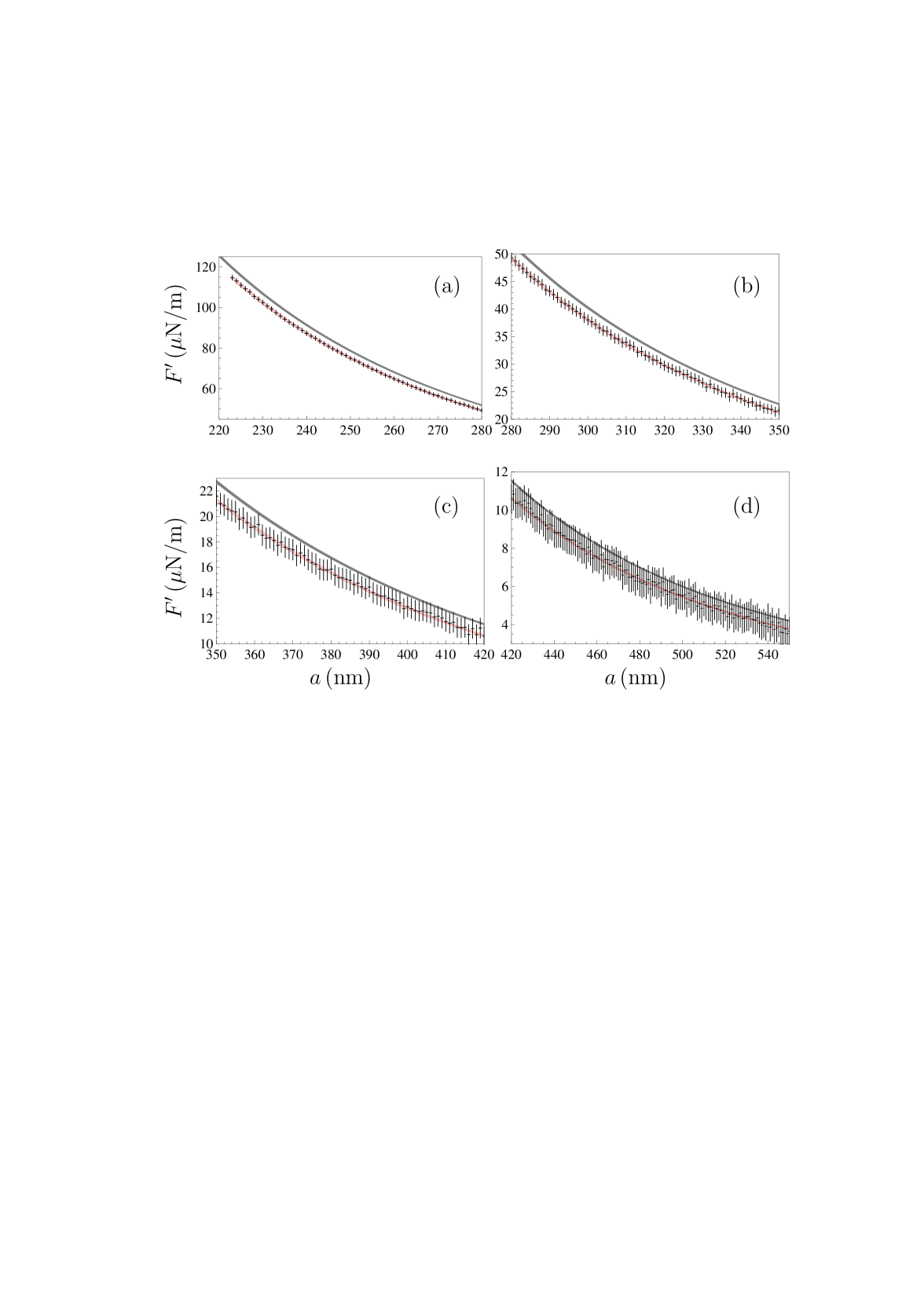
Figure 4: The mean measured gradients of the Casimir force between a sphere and a plate coated with magnetic metal Ni are shown by the crosses as functions of separation. The bottom and top theoretical bands are computed within the Lifshitz theory using the alternative nonlocal response functions and local Drude function, respectively.

The theoretical predictions of the Lifshitz theory computed 32 using the local dielectric response given by the Drude function ${\varepsilon}_{l}^{D}$ in Eq. (54) are shown by the top bands in Figs. 4(a)–4(d). Although the Drude response function takes proper account of the relaxation properties of conduction electrons in the on-shell electromagnetic fields, the theoretical predictions given by the top bands are excluded by the measurement data over the separation region from 223 to 420 nm. This can be explained by an assumption that the Drude function describes incorrectly the dielectric response to the off-shell electromagnetic fields contributing to the Casimir effect. One can conclude that the alternative nonlocal response functions provide a more adequate response to quantum fluctuations off the mass shell. Note that at separation distances below 100 nm the Casimir interaction is largely caused by the contribution of interband transitions to the dielectric permittivity. Because of this, at so short separations the discrimination between very close theoretical predictions obtained using the dielectric functions $\varepsilon^{D}$, $\varepsilon^{p}$, and $\varepsilon^{\rm Tr,L}$ is presently impossible and respective experiments are performed at larger separations (see Fig. 4 and Fig. 5 below).

We also use another approach to a comparison between experiment and theory based on the analysis of differences between theoretical gradients of the Casimir force (57) and mean measured gradients

$$\Delta F^{\prime}(a_{i},T)=F_{\rm theor}^{\prime}(a_{i},T)-F_{\rm expt}^{\prime}(a_{i},T),$$ (58)

where $a_{i}$ are the experimental separations at which the force gradient was measured.

     

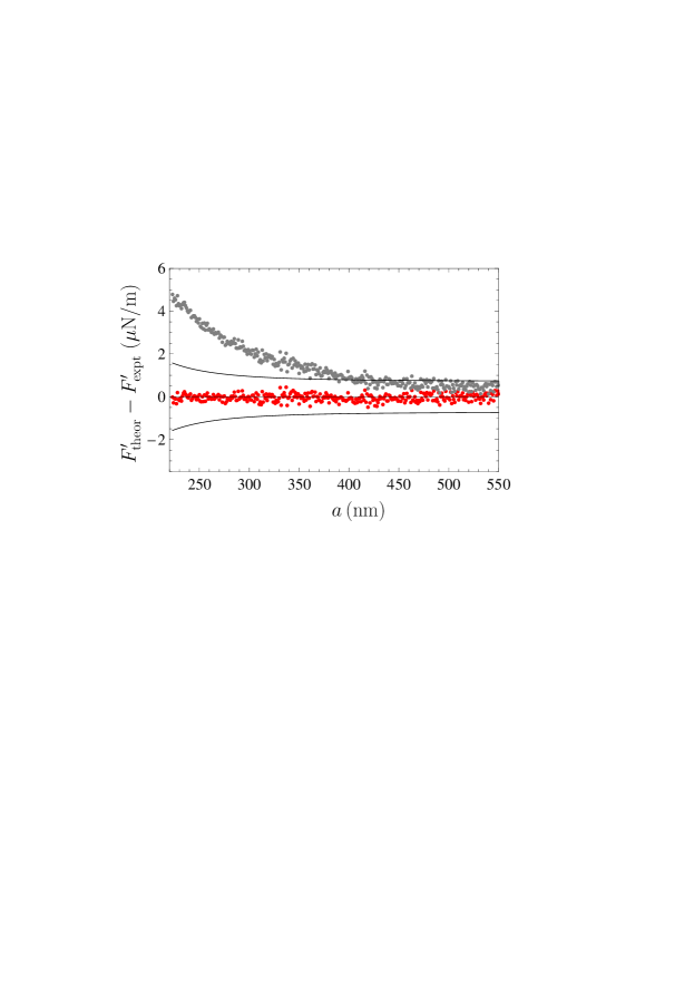
Figure 5: Differences between theoretical Casimir force gradients between a sphere and a plate coated with magnetic metal Ni computed either using the alternative nonlocal response functions (lower set of dots) or the local Drude function (upper set of dots) and mean experimental force gradients. The borders of the 67% confidence intervals for the force differences are shown by the two solid lines.

In Fig. 5, the lower set of dots presenting the quantity $\Delta F^{\prime}(a_{i},T)$ as a function of separation is computed with theoretical force gradients $F_{\rm theor}^{\prime}$ obtained using the alternative nonlocal response functions. For the upper set of dots the gradients $F_{\rm theor}^{\prime}$ were obtained using the local Drude response function. The two solid lines in Fig. 5 indicate the borders of the 67% confidence intervals for the random quantity $\Delta F^{\prime}$ in Eq. (58) which take into account the total experimental and theoretical errors.

As is seen in Fig. 5, all dots belonging to the lower set are inside the confidence intervals demonstrating a very good agreement between theory and the measurement data if the alternative nonlocal response functions are used in computations. The same holds when the local plasma response function is used in computations of $F_{\rm theor}^{\prime}$ 32 ; 33 which, however, disregards the relaxation properties of conduction electrons.

From Fig. 5 it is also seen that most of dots belonging to the upper set, obtained using the local Drude response function, are outside the confidence intervals over the separation region from 223 to 420 nm. This means that the Lifshitz theory using the local Drude response is experimentally excluded by measuring the Casimir interaction between magnetic metal plates.

According to the results of Sec. III, measurements of the Casimir interactions at separations of a few micrometers could easily discriminate between theoretical predictions of the Lifshitz theory obtained using the local plasma and the alternative nonlocal response functions. This could be made, for instance, by performing the differential force measurements proposed in Ref. 70 . At the moment, however, both these approaches to calculation of the Casimir force are experimentally consistent and one could decide between them based on only advantages and drawbacks in their application to a description of some other physical phenomena.

V Conclusions and discussion

In this paper, the Lifshitz theory of the Casimir force was extended to the case of magnetic metal boundary plates possessing a spatially nonlocal dielectric response. For this purpose, we have solved Maxwell equations describing an electromagnetic wave incident from vacuum on a magnetic metal semispace and expressed the exact impedances for two independent polarizations of the electromagnetic field via the longitudinal and transverse dielectric functions, as well as via the magnetic permeability of a semispace metal.

The obtained results were used to calculate the Casimir pressure between magnetic metal (Ni) plates described by the alternative nonlocal response functions. These functions have been introduced in Refs. 53 ; 54 in an effort to solve puzzling problems in the Lifshitz theory which was found to be in contradiction with the measurement data and fundamental principles of thermodynamics when the much studied relaxation properties of conduction electrons are taken into account in calculations by means of the Drude response function.

The basic idea behind introducing the alternative nonlocal response functions is that most of the experimental information about the electromagnetic response of a metal is obtained by using the on-shell fields. As to a nonlocal response to the off-shell fields, the possibilities of experimentally testing it are very limited. For instance, some information about only the longitudinal response function ${\varepsilon^{\,\rm L}}(\omega,{\mbox{\boldmath$k$}})$ can be obtained from measuring the energy loss and momentum transfer of a beam of high energy electrons passing through a thin metallic film 55 . This doubts on applications of the Drude response function with no modification in the region of electromagnetic fields off the mass shell, i.e., for $\omega^{2}<k^{2}c^{2}$, which gives a sizable contribution to the Casimir effect.

Thus, it is reasonable to look for nonlocal generalizations of the Drude function which nearly coincide with it for the on-shell fields but can deviate significantly for electromagnetic fluctuations off the mass shell. Taking into account that the plasma response function, leading to an agreement of the Lifshitz theory with the experimental data and requirements of thermodynamics, possesses the second order pole at zero frequency, the same property might be expected from the sought for response. The phenomenological alternative response functions introduced in Refs. 53 ; 54 satisfy these conditions.

Another motivation for using the alternative nonlocal response functions comes from graphene. At low energies characteristic for the Casimir effect at not too short separations, graphene is well described by the Dirac model. In the framework of this model, the spatially nonlocal response functions of graphene to both the on-shell and off-shell fields can be expressed precisely based on first principles of quantum field theory at nonzero temperature via the components of the polarization tensor in (2+1)-dimensional space-time (see Refs. 71 ; 72 for the complete results). In this situation, one expects that the Lifshitz theory of the Casimir interaction with graphene using its exact response functions should be in agreement with both the measurement data and requirements of thermodynamics. These expectations were confirmed by the measurement data of two experiments which were found to be in excellent agreement with theoretical predictions using the polarization tensor 73 ; 74 ; 75 ; 75a . On the other hand, the Casimir entropy in graphene systems calculated using the polarization tensor was proven to be in perfect agreement with the Nernst heat theorem 76 ; 77 ; 78 ; 79 .

After this discussion, we return to the obtained results. It was shown that at the experimental separations from 100 to 800 nm the Casimir pressures between two parallel Ni plates computed by the Lifshitz formula using the alternative nonlocal and local plasma response functions differ by less than 1%. However, at separations of a few micrometers these two theoretical predictions differ between themselves and with the prediction obtained using the local Drude function by several tens of percent. This opens up possibilities to experimentally check these predictions in near future.

We have also compared theoretical gradients of the Casimir force between a Ni-coated sphere and a Ni-coated plate, computed using the alternative nonlocal response functions and the optical data of Ni, with the measurement data of Refs. 32 ; 33 . The obtained theoretical results were found in to be in a very good agreement with the experimental ones over the entire range of separations from 223 to 550 nm. This agreement is almost identical to that obtained in Refs. 32 ; 33 using the optical data of Ni supplemented by the dissipationless plasma response function at low frequencies 32 ; 33 . It has been known also 32 ; 33 that the theoretical predictions obtained using the local Drude response are excluded by the measurement data over the range of separations from 223 to 420 nm. In so doing an advantage of the alternative nonlocal response functions is that they take into account the relaxation properties of conduction electrons at low frequencies, as does the Drude function, but, as opposed to the Drude function, leads to an agreement between experiment and theory which could be previously reached only by using the plasma model, i.e., by dropping the relaxation properties of conduction electrons.

In view of the above, one can conclude that the alternative nonlocal response functions to quantum fluctuations offer certain advantages over more conventional local response functions and deserve further investigation.

References

- (1) H. B. G. Casimir, On the attraction between two perfectly conducting bodies, Proc. Kon. Ned. Akad. Wet. B 51, 793 (1948).
- (2) I. Brevik and H. Kolbenstvedt, The Casimir effect in a solid ball when , Ann. Phys. (NY) 143, 179 (1982).
- (3) K. A. Milton, Fermionic Casimir stress on a spherical bag, Ann. Phys. (NY) 150, 432 (1983).
- (4) P. Candelas and S. Weinberg, Calculation of gauge couplings and compact circumferences from self-consistent dimensional reduction, Nucl. Phys. B 237, 397 (1984).
- (5) L. H. Ford, Quantum vacuum energy in general relativity, Phys. Rev. D 11, 3370 (1975).
- (6) S. G. Mamaev, V. M. Mostepanenko, and A. A. Starobinskii, Particle creation from the vacuum near a homogeneous isotropic singularity, Zh. Eksp. Teor. Fiz. 70, 1577 (1976) [Sov. Phys. JETP 43, 823 (1976)].
- (7) V. B. Bezerra, G. L. Klimchitskaya, V. M. Mostepanenko, and C. Romero, Advance and prospects in constraining the Yukawa-type corrections to Newtonian gravity from the Casimir effect, Phys. Rev. D 81, 055003 (2010).
- (8) G. L. Klimchitskaya and V. M. Mostepanenko, Constraints on axionlike particles and non-Newtonian gravity from measuring the difference of Casimir forces, Phys. Rev. D 95, 123013 (2017).
- (9) G. L. Klimchitskaya, P. Kuusk, and V. M. Mostepanenko, Constraints on non-Newtonian gravity and axionlike particles from measuring the Casimir force in nanometer separation range, Phys. Rev. D 101, 056013 (2020).
- (10) P. W. Milonni, The Quantum Vacuum. An Introduction to Quantum Electrodynamics (Academic Press, San Diego, 1994).
- (11) G. L. Klimchitskaya, U. Mohideen, and V. M. Mostepanenko, The Casimir force between real materials: Experiment and theory, Rev. Mod. Phys. 81, 1827 (2009).
- (12) A. W. Rodrigues, F. Capasso, and S. G. Johnson, The Casimir effect in microstructured geometries, Nat. Photon. 5, 211 (2011).
- (13) M. Bordag, G. L. Klimchitskaya, U. Mohideen, and V. M. Mostepanenko, Advances in the Casimir Effect (Oxford University Press, Oxford, 2015).
- (14) L. M. Woods, D. A. R. Dalvit, A. Tkatchenko, P. Rodriguez-Lopez, A. W. Rodriguez, and R. Podgornik, Materials perspective on Casimir and van der Waals interactions, Rev. Mod. Phys. 88, 045003 (2016).
- (15) S. Y. Buhmann, Disperson Forces, I,II (Springer, Berlin, 2012).
- (16) Bo E. Sernelius, Fundamentals of van der Waals and Casimir Interactions (Springer, New York, 2018).
- (17) N. G. Van Kampen, B. R. A. Nijboer, and K. Schram, On the macroscopic theory of Van der Waals forces, Phys. Lett. A 26, 307 (1968).
- (18) B. W. Ninham, V. A. Parsegian, and G. H. Weiss, On the macroscopic theory of temperature-dependent van der Waals forces, J. Stat. Phys. 2, 323 (1970).
- (19) D. Langbein, Macroscopic theory of van der Waals attraction, Solid State Commun. 12, 853 (1973).
- (20) K. Schram, On the macroscopic theory of retarded Van der Waals forces, Phys. Lett. A 43, 282 (1973).
- (21) K. A. Milton, The Casimir Effect: Physical Manifestations of Zero-Point Energy (World Scientific, Singapore, 2001).
- (22) E. M. Lifshitz, The theory of molecular attractive forces between solids, Zh. Eksp. Teor. Fiz. 29, 94 (1955) [Sov. Phys. JETP 2, 73 (1956)].
- (23) E. M. Lifshitz and L. P. Pitaevskii, Statistical Physics, Part II (Pergamon, Oxford, 1980).
- (24) P. Richmond and B. W. Ninham, A note on the extension of the Lifshitz theory of van der Waals forces to magnetic media, J. Phys. C: Solid St. Phys. 4, 1988 (1971).
- (25) Yu. S. Barash and V. L. Ginzburg, Electromagnetic fluctuations in a substance and molecular (van der Waals) interbody forces, Usp. Fiz. Nauk 116, 5 (1975) [Sov. Phys. Usp. 18, 305 (1975)].
- (26) R. S. Decca, E. Fischbach, G. L. Klimchitskaya, D. E. Krause, D. López, and V. M. Mostepanenko, Improved tests of extra-dimensional physics and thermal quantum field theory from new Casimir force measurements, Phys. Rev. D 68, 116003 (2003).
- (27) R. S. Decca, D. López, E. Fischbach, G. L. Klimchitskaya, D. E. Krause, and V. M. Mostepanenko, Precise comparison of theory and new experiment for the Casimir force leads to stronger constraints on thermal quantum effects and long-range interactions, Ann. Phys. (NY) 318, 37 (2005).
- (28) R. S. Decca, D. López, E. Fischbach, G. L. Klimchitskaya, D. E. Krause, and V. M. Mostepanenko, Tests of new physics from precise measurements of the Casimir pressure between two gold-coated plates, Phys. Rev. D 75, 077101 (2007).
- (29) R. S. Decca, D. López, E. Fischbach, G. L. Klimchitskaya, D. E. Krause, and V. M. Mostepanenko, Novel constraints on light elementary particles and extra-dimensional physics from the Casimir effect, Eur. Phys. J. C 51, 963 (2007).
- (30) C.-C. Chang, A. A. Banishev, R. Castillo-Garza, G. L. Klimchitskaya, V. M. Mostepanenko, and U. Mohideen, Gradient of the Casimir force between Au surfaces of a sphere and a plate measured using an atomic force microscope in a frequency-shift technique, Phys. Rev. B 85, 165443 (2012).
- (31) A. A. Banishev, C.-C. Chang, G. L. Klimchitskaya, V. M. Mostepanenko, and U. Mohideen, Measurement of the gradient of the Casimir force between a nonmagnetic gold sphere and a magnetic nickel plate, Phys. Rev. B 85, 195422 (2012).
- (32) A. A. Banishev, G. L. Klimchitskaya, V. M. Mostepanenko, and U. Mohideen, Demonstration of the Casimir Force between Ferromagnetic Surfaces of a Ni-Coated Sphere and a Ni-Coated Plate, Phys. Rev. Lett. 110, 137401 (2013).
- (33) A. A. Banishev, G. L. Klimchitskaya, V. M. Mostepanenko, and U. Mohideen, Casimir force between two magnetic metals in comparison with nonmagbetic test bodies, Phys. Rev. B 88, 155410 (2013).
- (34) G. Bimonte, D. López, and R. S. Decca, Isoelectronic determination of the thermal Casimir force, Phys. Rev. B 93, 184434 (2016).
- (35) J. Xu, G. L. Klimchitskaya, V. M. Mostepanenko, and U. Mohideen, Reducing detrimental electrostatic effects in Casimir-force measurements and Casimir-force-based microdevices, Phys. Rev. A 97, 032501 (2018).
- (36) M. Liu, J. Xu, G. L. Klimchitskaya, V. M. Mostepanenko, and U. Mohideen, Examining the Casimir puzzle with an upgraded AFM-based technique and advanced surface cleaning, Phys. Rev. B 100, 081406(R) (2019).
- (37) M. Liu, J. Xu, G. L. Klimchitskaya, V. M. Mostepanenko, and U. Mohideen, Precision measurements of the gradient of the Casimir force between ultraclean metallic surfaces at larger separations, Phys. Rev. A 100, 052511 (2019).
- (38) G. Bimonte, B. Spreng, P. A. Maia Neto, G.-L. Ingold, G. L. Klimchitskaya, V. M. Mostepanenko, and R. S. Decca, Measurement of the Casimir Force between 0.2 and m: Experimental Procedures and Comparison with Theory, Universe 7, 93 (2021).
- (39) V. B. Bezerra, G. L. Klimchitskaya, V. M. Mostepanenko, and C. Romero, Violation of the Nernst heat theorem in the theory of thermal Casimir force between Drude metals, Phys. Rev. A 69, 022119 (2004).
- (40) M. Bordag and I. Pirozhenko, Casimir entropy for a ball in front of a plane, Phys. Rev. D 82, 125016 (2010).
- (41) G. L. Klimchitskaya and V. M. Mostepanenko, Low-temperature behavior of the Casimir free energy and entropy of metallic films, Phys. Rev. A 95, 012130 (2017).
- (42) G. L. Klimchitskaya and C. C. Korikov, Analytic results for the Casimir free energy between ferromagnetic metals, Phys. Rev. A 91, 032119 (2015).
- (43) S. Boström and Bo E. Sernelius, Entropy of the Casimir effect between real metal plates, Physica A 339, 53 (2004).
- (44) I. Brevik, J. B. Aarseth, J. S. Høye, and K. A. Milton, Temperature dependence of the Casimir effect, Phys. Rev. E 71, 056101 (2005).
- (45) J. S. Høye, I. Brevik, S. A. Ellingsen, and J. B. Aarseth, Analytical and numerical verification of the Nernst theorem for metals, Phys. Rev. E 75, 051127 (2007).
- (46) V. M. Mostepanenko, Casimir Puzzle and Conundrum: Discovery and Search for Resolution, Universe 7, 84 (2021).
- (47) J. Lindhard, On the properties of a gas of charged particles, Dan. Mat. Fys. Medd. 28, 1 (1954).
- (48) V. P. Silin and E. P. Fetisov, Electromagnetic properties of a relativistic plasma, III, Zh. Eksp. Teor. Fiz. 41, 159 (1961) [Sov. Phys. JETP 14, 115 (1962)].
- (49) K. L. Kliewer and R. Fuchs, Anomalous Skin Effect for Specular Electron Scattering and Optical Experiments at Non-Normal Angles of Incidence, Phys. Rev. 172, 607 (1968).
- (50) N. D. Mermin, Lindhard Dielectric Function in the Relaxation Time Approximation, Phys. Rev. B 1, 2362 (1970).
- (51) E. I. Kats, Influence of nonlocality effects on van der Waals interaction, Zh. Eksp. Teor. Fiz. 73, 212 (1977) [Sov. Phys. JETP 46, 109 (1977)].
- (52) R. Esquivel and V. B. Svetovoy, Correction to the Casimir force due to the anomalous skin effect, Phys. Rev. A 69, 062102 (2004).
- (53) G. L. Klimchitskaya and V. M. Mostepanenko, An alternative response to the off-shell quantum fluctuations: a step forward in resolution of the Casimir puzzle, Eur. Phys. J. C 80, 900 (2020).
- (54) G. L. Klimchitskaya and V. M. Mostepanenko, Casimir entropy and nonlocal response functions to the off-shell quantum fluctuations, Phys. Rev. D 103, 096007 (2021).
- (55) M. Dressel and G. Grüner, Electrodynamics of Solids: Optical Properties of Electrons in Metals (Cambridge University Press, Cambridge, 2003).
- (56) L. D. Landau, E. M. Lifshitz, and L. P. Pitaevskii, Electrodynamics of Continuous Media (Pergamon, Oxford, 1984).
- (57) Handbook of Optical Constants of Solids, edited by E. D. Palik (Academic Press, New York, 1985).
- (58) M. A. Ordal, R. J. Bell, R. W. Alexander, L. L. Long, and M. R. Querry, Optical properties of fourteen metals in the infrared and far infrared: Al, Co, Cu, Au, Fe, Pb, Mo, Ni, Pd, Pt, Ag, Ti, V, and W, Appl. Optics 24, 4493 (1985).
- (59) A. Goldman, Handbook of Modern Ferromagnetic Materials (Springer, New York, 1999).
- (60) B. Geyer, G. L. Klimchitskaya, and V. M. Mostepanenko, Thermal Casimir interaction between two magnetodielectric plates, Phys. Rev. B 81, 104101 (2010).
- (61) R. Esquivel, C. Villarreal, and W. L. Mochán, Exact surface impedance formulation of the Casimir force: Application to spatially dispersive metals, Phys. Rev. A 68, 052103 (2003); 71, 029904(E) (2005).
- (62) M. Bordag, G. L. Klimchitskaya, and V. M. Mostepanenko, The Casimir force between plates with small deviations from plane-parallel geometry, Int. J. Mod. Phys. A 10, 2661 (1995).
- (63) P. J. van Zwol, G. Palasantzas, and J. Th. M. De Hosson, Influence of random roughness on the Casimir force at small separations, Phys. Rev. B 77, 075412 (2008).
- (64) C. D. Fosco, F. C. Lombardo, and F. D. Mazzitelli, Proximity force approximation for the Casimir energy as a derivative expansion, Phys. Rev. D 84, 105031 (2011).
- (65) G. Bimonte, T. Emig, R. L. Jaffe, and M. Kardar, Casimir forces beyond the proximity force approximation, Europhys. Lett. 97, 50001 (2012).
- (66) G. Bimonte, T. Emig, and M. Kardar, Material dependence of Casimir force: gradient expansion beyond proximity, Appl. Phys. Lett. 100, 074110 (2012).
- (67) L. P. Teo, Material dependence of Casimir interaction between a sphere and a plate: First analytic correction beyond proximity force approximation, Phys. Rev. D 88, 045019 (2013).
- (68) G. Bimonte, Going beyond PFA: A precise formula for the sphere-plate Casimir force, Europhys. Lett. 118, 20002 (2017).
- (69) M. Hartmann, G.-L. Ingold, and P. A. Maia Neto, Plasma versus Drude Modeling of the Casimir Force: Beyond the Proximity Force Approximation, Phys. Rev. Lett. 119, 043901 (2017).
- (70) G. Bimonte, G. L. Klimchitskaya, and V. M. Mostepanenko, Universal experimental test for the role of free charge carriers in the thermal Casimir effect within a micrometer separation range, Phys. Rev. A 95, 052508 (2017).
- (71) M. Bordag, G. L. Klimchitskaya, V. M. Mostepanenko, and V. M. Petrov, Quantum field theoretical description for the reflectivity of graphene, Phys. Rev. D 91, 045037 (2015); 93, 089907(E) (2016).
- (72) M. Bordag, I. Fialkovskiy, and D. Vassilevich, Enhanced Casimir effect for doped graphene, Phys. Rev. B 93, 075414 (2016); 95, 119905(E) (2017).
- (73) A. A. Banishev, H. Wen, J. Xu, R. K. Kawakami, G. L. Klimchitskaya, V. M. Mostepanenko, and U. Mohideen, Measuring the Casimir force gradient from graphene on a SiO2 substrate, Phys. Rev. B 87, 205433 (2013).
- (74) G. L. Klimchitskaya, U. Mohideen, and V. M. Mostepanenko, Theory of the Casimir interaction for graphene-coated substrates using the polarization tensor and comparison with experiment, Phys. Rev. B 89, 115419 (2014).
- (75) M. Liu, Y. Zhang, G. L. Klimchitskaya, V. M. Mostepanenko, and U. Mohideen, Demonstration of an Unusual Thermal Effect in the Casimir Force from Graphene, Phys. Rev. Lett. 126, 206802 (2021).
- (76) M. Liu, Y. Zhang, G. L. Klimchitskaya, V. M. Mostepanenko, and U. Mohideen, Experimental and theoretical investigation of the thermal effect in the Casimir interaction from graphene, Phys. Rev. B 104, 085436 (2021).
- (77) G. L. Klimchitskaya and V. M. Mostepanenko, Low-temperature behavior of the Casimir-Polder free energy and entropy for an atom interacting with graphene, Phys. Rev. A 98, 032506 (2018).
- (78) G. L. Klimchitskaya and V. M. Mostepanenko, Nernst heat theorem for an atom interacting with graphene: Dirac model with nonzero energy gap and chemical potential, Phys. Rev. D 101, 116003 (2020).
- (79) G. L. Klimchitskaya and V. M. Mostepanenko, Quantum field theoretical description of the Casimir effect between two real graphene sheets and thermodynamics, Phys. Rev. D 102, 016006 (2020).
- (80) G. L. Klimchitskaya and V. M. Mostepanenko, Casimir and Casimir-Polder Forces in Graphene Systems: Quantum Field Theoretical Description and Thermodynamics, Universe 6, 150 (2020).