Reinforcement Learning for Admission Control in Wireless Virtual Network Embedding

Abstract

Using Service Function Chaining (SFC) in wireless networks became popular in many domains like networking and multimedia. It relies on allocating network resources to incoming SFCs requests, via a Virtual Network Embedding (VNE) algorithm, so that it optimizes the performance of the SFC. When the load of incoming requests – competing for the limited network resources – increases, it becomes challenging to decide which requests should be admitted and which one should be rejected.

In this work, we propose a deep Reinforcement learning (RL) solution that can learn the admission policy for different dependencies, such as the service lifetime and the priority of incoming requests. We compare the deep RL solution to a first-come-first-serve baseline that admits a request whenever there are available resources. We show that deep RL outperforms the baseline and provides higher acceptance rate with low rejections even when there are enough resources.

I Introduction

Network Function Virtualization (NFV) is a common trend in networking as seen in telecommunications [1], Multimedia [2] and cloud computing [3]. One of its key roles is to embed a chain of services, also known as Service Function Chain (SFC), into infrastructure networks. The process of embedding is defined as Virtual Network Embedding (VNE), where a controller receives a Virtual Network Request (VNR) to allocate resources (e.g., CPU capacities and routes) to these services.

It becomes challenging when these VNRs have different minimum resource requirements. In this case, multiple VNRs are competing for the finite resources of infrastructure networks. A VNE algorithm can only allocate resources to optimize the performance of new incoming VNRs, but it cannot terminate an embedded VNR to accept new ones. Consequently, we need to control the admission of these VNRs into the infrastructure to decide which VNRs should be embedded. A possible naive, greedy, solution is to admit a VNR that can be served at the time of request, i.e., First Come First Serve.

Meanwhile, when the services differ in required resources, value or importance, the naive solution runs the risk of admitting less valuable, more resource-hungry services only to reject several other upcoming VNRs. We are hence interested in an admission control approach for VNRs, which optimizes the long-term average of admitted services (possibly weighted by revenue, value, priority, etc.) rather than just myopically focusing on the current request.

As this needs an understanding of upcoming requests, explicit models for that are usually not available, reinforcement learning is a promising approach. In this work, we use VNE in Wireless Sensor Network (WSN) as a case study and use two parameters to describe incoming VNRs:

• service lifetime: duration of leasing the network resources

• priority of embedding a VNR

Such applications are seen in smart environments with few to many distributed smart devices. These devices are supported by sensors that generate VNRs for heavy processing (seen in, e.g., gaming and multimedia applications) that can be executed on the near-by smart devices. We hence investigate RL as a tool for admission control of VNRs, where the uncertainty of upcoming VNRs is the main challenge. This could be related to, for example, changing arrival rates or VNRs parameters. We focus here on the latter, so that VNRs have different service lifetime and different priorities. The main objective of admission control is then to embed as many VNRs as possible (or VNRs with higher revenues), averaged over long time. For fairness and to avoid abusing the resources, an embedded VNR is terminated if its service lifetime ends.

In the following sections, we give a brief overview of related work with respect to admission control and Reinforcement Learning (RL), and how it differs from our work (Section II). Then, we formulate the problem and summarize the applied VNE solution (Section III). Next, we describe our RL framework (Section IV) and compare the proposed solution to greedy admission control in different simulation setups (Section V). Finally, we summarize the outcome in Section VII

II Related work

Using an RL approach in the context of WSNs has been used to solve many problems as in Medium Access Control (MAC) [4], energy saving [5], and many other similar problems [3]. Meanwhile, we focus here on work that explicitly consider RL, VNE and admission control.

Different types of requests were investigated when using RL for admission control. For instance, the authors in [6, 7, 8] assume that incoming requests have flow properties that need to be completed before some deadline, while the authors in [9, 10] assume that incoming requests are jobs that need to be running on servers, e.g., cloud or edge servers. In our work, the requests have the properties of both jobs and flows, since a VNR has multiple jobs connected via link flows.

The authors in [11, 12] assume that Quality of Service (QoS) is a constraint, hence, their proposed solutions reject VNRs that are likely to violate QoS bounds. In contrast to their assumption, we assume that QoS is an objective for the VNE problem, while the admission control maximizes the embedding revenue.

Furthermore, the work in [12] assumed arriving VNRs wait in a queue for a decision to be embedded or to be rejected. Meanwhile, in our work, and similar to [11], we have a queue length of only one. Therefore, queuing issues have been ignored to emphasize other features of the admission control problem. Consequently, using RL for optimizing waiting time in the queue [8, 13], queue length [14] and queuing management [15] is beyond the scope of this paper.

We use a VNE solution to check the feasibility of embedding a VNR. To combine both admission control and VNE problems, the work in [16] uses recurrent neural networks to reject VNRs that are likely to fail the QoS constraints, which saves the computational time needed by the VNE solution to check the VNR implementation feasibility. Hence, the admission control was trained to have high accuracy of detecting feasible accepted VNR embedding. In our work, the admission control is trained to maximize the network’s revenue, meaning that it can reject feasible VNRs in order to accept more VNRs later. Using [16] as a quick feasibility check and then using our RL agent to reject unpromising requests should make an interesting followup study.

Another prediction model was used by [17] to predict the arrival rate of upcoming VNRs. This is then followed by an RL agent, whose objective is to maximize the acceptance rate. In contrast, we do not use the arrival rate as an observation so that it is being implicitly learned by the RL agent. Building up on our work to consider changing arrival rates is straight forward, yet it requires deep analyses with respect to the uncertainty of the changes and the performance, which we leave as an extension to this work.

Further combinations of admission control and VNE decisions have been solved using RL in [18, 19]. Similar to our work, the objective is to maximize the network’s revenue. The monolithic mix of VNE and admission control applied in [18] is valid only for wired networks and cannot be applied or reused in our wireless network, due to the differences between wired and wireless VNE problems [20]. However, we assume a modular implementation, where admission control and VNE solutions are two separate modules that interact with each other. This allows reusing different modules in similar problems. Additionally, the simplicity of our problem will probably lead to shorter training time and faster convergence [21].

III Problem formulation

There are two objectives for our problem. First, we need to maximize the revenue from accepting VNRs, which is based on the acceptance rate, service time or/and priority of VNRs. Second, we need to minimize the number of used time slots per an accepted VNR for a high QoS. The latter is solved by a heuristic VNE solution (Section III-D). Because of our modular implementation, this VNE solution is treated as a black box to our first objective (Figure 1).

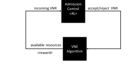
Figure 1: Interaction between VNE and admission control

The first objective –our main focus in this paper– would require rejecting VNRs, even if they could be embedded by the VNE solution, to allow more/better upcoming VNRs to be embedded instead. Hence, the decisions of whether to accept/reject a VNE depends on the resource allocation but not vice versa.

In the following subsections, we describe the features of the VNRs and the wireless network for formulating our problem, and describe briefly the VNE solution, since it interacts with the admission control.

III-A Virtual network requests

A VNR consists of $B$ tasks connected via $E$ links. Each processing task $b\in B$ requires a capacity $c_{\mathrm{req}}^{b}$, while a link has a minimum transmission data rate $r_{\mathrm{req}}$ requirement.

We assume that we have a predefined set of VNRs, whose typologies are known in advance. Hence, each VNR is labeled with an Identifier (ID), where the duration and priority of each VNR can change, but the topology and required resources do not.

Additionally, we assume that we have a discrete time environment, where at each time slot a new VNR $v$ arrives, whose runtime $\delta^{v}$ is uniformly distributed between $\left[\delta_{\mathrm{min}},\delta_{\mathrm{max}}\right]$ time steps. By altering the value of $\delta_{\mathrm{max}}$, the average VNR duration can be adjusted to simulate different loads. Similarly, each VNR has a priority $\lambda^{v}\in\left[\lambda_{\mathrm{min}},\lambda_{\mathrm{max}}\right]$.

III-B Wireless Sensor Network

The wireless sensor nodes operate in half-duplex communication mode; a node can be in one of three states: send, receive, idle. Each node $p\in P$ is defined using this set of properties: position in network computational capacity $C^{p}$, transmit power $S^{p}$ and noise floor $N_{0}$.

We assume that all sensor nodes share the same collision domain with bandwidth $\mathrm{BW}$. To allow multiple channel access, we assume an ideal TDMA with no collision and all transmissions are synchronized, in which we have $T$ time slots.

Given the attenuation $\gamma^{i,j}$ between two nodes $i,j\in P$ , the maximum achievable data rate $r_{\mathrm{max}}^{i,j,t}$ at time slot $t\in T$ is given by

$$r_{\mathrm{max}}^{i,j,t}=\frac{\mathrm{BW}}{|T|}\mathrm{log_{2}}(1+\frac{S^{i}\gamma^{i,j}}{I^{i,j,t}+N_{0}})$$ (1)

where $I^{i,j,t}=\sum_{\begin{subarray}{c}p\in P^{t}\\ p\neq i\end{subarray}}\gamma^{p,j}S^{p}$ is the interference at node $j$ from other nodes $P^{t}$ that are simultaneously transmitting with node $i$ at time slot $t$.

III-C Constraints

The required constraints for successful wireless VNE are described in details in [20], but we summarize them here whilst extending the formulation to a discrete time horizon.

First, a successfully embedded VNR $v$ will decrease its time duration $\delta^{v}=\delta^{v}-1$ each time step, so that $v$ is running as long as $\delta^{v}>0$, otherwise, the VNR will be terminated to avoid additional costs or abusing the resources. Second, let us assume that we have a list of VNRs $V^{+}$ which are currently running inside the network (i.e., $\delta^{v}>0,\quad\forall v\in V^{+}$). Then, we need to ensure the following

$$\sum_{P}\theta(b^{v},p) = 1 ,\quad\forall b\in v,\forall v\in V^{+}$$ (2)

$$\sum_{b\in B}\theta(b^{v},p)c_{\mathrm{req}}^{b} \leq C^{p} ,\quad\forall v\in V^{+},\forall p\in P$$ (3)

$$\eta(e^{v},i,j,t)r_{\mathrm{req}}^{e^{v}} \leq r_{\mathrm{max}}^{i,j,t}, \quad\forall\left\{i,j\right\}\in P,t\in T,e\in E,v\in V^{+}~{}$$ (4)

We use two binary variables to formulate the constraints: $\theta(b,p)$ and $\eta(e,i,j,t)$. The former is used to state if task $b$ is running on node $p$, while the latter is used to state if node $i$ is transmitting to node $j$ the data of link $e$ at time slot $t$.

In Eq. (2), we ensure that each task $b\in B$ where $v\in V^{+}$ is running on a node. However, all nodes should not be overutilized (Eq. (3)). Similarly, to guarantee an upper-bound delay, Eq. (4) checks, if node $i$ is transmitting the link $e$ to node $j$ at time slot $t$, then $r_{\mathrm{req}}^{e}$ is less than or equal to the maximum achievable rate $r_{\mathrm{max}}^{i,j,t}$. Note that we assume, for simplicity, a perfect medium access channel with constant channel access delay. Based on the interference from different transmissions, two nodes may transmit data of different links simultaneously.

In addition to the above constraints, we check the flow conservation ones to ensure successful routing. Meanwhile, we drop the formulation of these constraints lest we distract from the goal of the paper; the reader is referred to [22] for a detailed description.

III-D VNE solution

Our VNE solution is a straightforward first-fit constructive heuristic [22], which finds a solution by following a sequence of pre-ordered constraints. We summarize the process as following. First, wireless nodes are chosen at random for running the tasks on nodes, while checking the capacity constraint. If any node does not satisfy the capacity constraint, another node is selected at random. Next, we find shortest path routes between the nodes running the tasks. At the end, time slots are allocated to the transmissions between the nodes in a topological order. We start at the beginning with one time slot. If simultaneous transmissions cannot take place within the available time slots –i.e., due to duplex or $\mathrm{SINR}$ constraints –new additional time slots are used for transmissions. The optimality gap of this heuristic has been derived in [22].

IV Reinforcement learning for admission control

In this section, we describe the RL implementation of the admission control. As shown in Figure 1, the VNE solution, described in Section III-D, acts as an RL environment. Accordingly, it additionally provides the controller with a reward for training purposes.

In the following subsections, we define the observation space, action space and reward function of the RL environment.

IV-A Observation space

All observations are stored in a fixed-size multi discrete vector containing the following information:

• Node capacities: $\rightarrow\mathbb{R}^{P}$

• Edge activation $\equiv\eta$ $\rightarrow$ $\mathbb{R}^{P\times P\times T\times 2}$

• New VNR properties $\rightarrow\mathbb{R}^{2}$

  • Service time

  • Priority

Node capacities contain the available capacities of each node at the current time step. Edge activation is a multi-dimensional matrix containing all currently embedded links. The first and second dimension encode the edge of sending and receiving nodes. The third dimension stands for the time step at which the transmission takes place. Each transmission is labeled by 2 IDs representing which VNR and which link within the VNR. For new incoming VNRs, we add the VNR ID, duration $\delta^{v}$ and priority $\lambda^{v}$

IV-B Action space

The RL agent decides whether an incoming VNR is rejected or accepted (binary space). In case of acceptance, the VNE algorithm will try to embed the VNR into the network.

IV-C Reward function

The reward function is modeled to train the agent towards the desired behavior described in III.

TABLE I: Reward function

Agent decision	VNE solution	Label	Reward
accepted	feasible	true positive	+6
accepted	infeasible	false positive	-2
rejected	feasible	false negative	-1 + $r_{\mathrm{extra}}$
rejected	infeasible	true negative	±0

Table I describes the combinations of agent decisions and VNE algorithm solutions with their corresponding reward. An incoming VNR is labeled as true positive, if the agent decides to accept theVNR and the VNE algorithm successfully embedded it. The other labels describe the remaining combinations of agent’s decisions and the VNE solution feasibility. Note that these labels are just used to highlight the differences in taken decisions between the RL and first-come-first-serve solutions and do not reflect the performance of the RL decisions.

False negatives receive a positive reward $r_{\mathrm{extra}}$ calculated using Eq. (5), which stimulates accepting VNRs with high priority and low service lifetime. It relies on the relative delay ($f_{\delta}^{v}=\frac{\delta^{v}}{\delta_{\mathrm{max}}}$) and the relative priority ($f_{\lambda}^{v}=\frac{\lambda_{\mathrm{max}}-\lambda^{v}}{\lambda_{\mathrm{max}}-1}$) of the rejected VNR $v$.

$$r_{\mathrm{extra}}^{v}=c_{\delta}\cdot f_{\delta}^{v}+c_{\lambda}\cdot f_{\lambda}^{v}$$ (5)

The control parameters $c_{\delta}$ and $c_{\lambda}$ are used to tune the false negative behavior on the extra reward. In other words, they tune the weights for acceptance rate and the revenue.

V Simulation setup

The VNR used in this paper is made of three processing tasks ${B=\left\{\mathrm{K},\mathrm{L},\mathrm{M}\right\}}$ connected via two links ($E=\left\{\mathrm{KL},\mathrm{LM}\right\}$) as shown in Fig. 2.

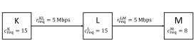
Figure 2: VNR overlay graph

The number of time slots per time step is $T=8$ for all simulations in this paper. We simulate 5 nodes placed in a small room (e.g., an office) with dimensions $3\,$\mathrm{m}$\,\times\,3\,$\mathrm{m}$,\times 3\,$\mathrm{m}$$. The wireless channel bandwidth is set to $\mathrm{BW}=20\,$\mathrm{M}\mathrm{H}\mathrm{z}$$. We set the minimum time duration per VNR $\delta_{\mathrm{min}}=2$ and $\delta_{\mathrm{max}}=30$, while the the VNR’s priority $\lambda\in\left[1,10\right]$.

All trained agents are compared to a baseline that always accepts a VNR and embed it whenever there are enough resources. Accordingly, this will have the first-come-first-serve behavior, where the embedding of a VNR depends only on the VNE solution’s feasibility. With respect to Table I, the output of this algorithm corresponds only to true positives and false positives.

To measure the impact of the control parameters ($c_{\delta}$ and $c_{\lambda}$) and the sensitivity of the trained agent to incoming VNR properties, we define 3 simulation setups:

1. fix $c_{\lambda}$ and change $c_{\delta}$

2. change $c_{\lambda}$ and fix $c_{\delta}$

3. fix both $c_{\lambda}$ and $c_{\delta}$, while evaluating different agents trained on different $\delta_{\mathrm{max}}$

VI Simulation results

We have for each configuration setup 100 different runs, where each run has 1000 time steps (i.e., 1000 incoming VNRs). We compare the median –to exclude outliers– of these runs to that from the baseline solution (gray dots).

VI-A Emphasizing low service time

As stated in Section IV-C, $c_{\delta}$ controls the agent’s decision (i.e., accept/reject a VNR $v$) with respect to the VNR’s duration $\delta^{v}$. To illustrate the sensitivity of agent’s decision to this parameter, we train eight agents whose $c_{\delta}$ change between $[1.6,3.0]$. All agents train for the same number of steps $10^{6}$ and $\delta_{\mathrm{max}}=30$ (Fig. 3).

Fig. 3a shows the median acceptance rate ($\frac{\text{number of accepted \acs{VNR}}}{\text{total number of incomming \acsp{VNR}}}$) of all trained agents and the always accept baseline agent under different offered load. Fig. 3b shows the corresponding relative number of false negatives created by those agents.

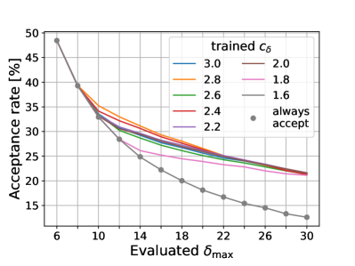
(a) Acceptance rate

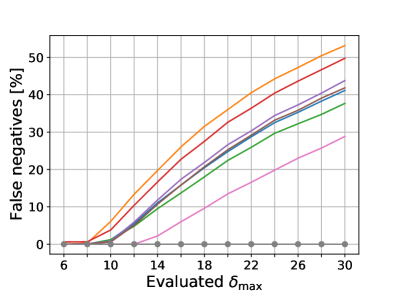
(b) False negatives

Figure 3: Results of $c_{\delta}$ parameter analysis

The agent trained with $c_{\delta}=1.6$ does not increase overall acceptance rate compared to the always accept baseline agent and does not make any false negatives decisions. Agents with higher values for $c_{\delta}$ show an increase in overall acceptance rate especially in higher offered load environments. This increase comes with the cost of creating more false negatives. The difference between each other is most present for medium offered loads. The agents with $c_{\delta}=1.8,2.0,2.2,2.4$ show a gradual increase in acceptance rate compared to each other when evaluating $\delta_{\mathrm{max}}$ between 10 and 22. For incoming VNRs with higher $\delta_{\mathrm{max}}$, the agents’ perform closely to each other (as in $c_{\mathrm{d}}=2.6,2.8,3.0$) to be twice as high as the baseline, while the unnecessary rejections introduced by the false negatives increases(Fig. 3b).

Consequently, $c_{\delta}$ should be carefully tuned: very small values will have similar performance to the baseline solution (lower bound), while having high values will yield unnecessary rejections and minimal to no gain in the acceptance ratio.

VI-B Emphasizing high priorities

Previous analyses focused on maximizing the acceptance rate by rejecting long VNRs. This may not be ideal because it prevents longer VNRs from being embedded at all. To prevent this, $c_{\lambda}$ can be used to give higher priority for longer VNRs (e.g., higher revenue). Fig. 4 shows the evaluation results of the trained agents with different values for $c_{\lambda}$ and $\lambda\in[1,10]$, while all agents use $\delta_{\mathrm{max}}=26$ for training and evaluations.

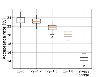
(a) Acceptance rate

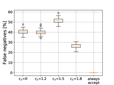
(b) False negatives

Figure 4: Results of $c_{\lambda}$ parameter analysis with $c_{\delta}=1.8$ and $\delta_{\mathrm{max}}=26$

In Fig. 4a, we observe that the higher the value of $c_{\lambda}$ during training the lower the acceptance of the resulting agent. This is due to accepting VNRs with high $\delta_{\mathrm{max}}$ and high priority. Meanwhile, there is a tendency to decrease the number of false negatives as $c_{\lambda}$ increases.

We extend our analysis, in Fig. 5, to investigate which VNRs are getting accepted or rejected during evaluation. Fig. 5a shows the number of true positives while Fig. 5b shows the number of false negatives using different values for $c_{\lambda}$ during training. Each point represents the number of embedded VNRs with their corresponding duration and priority values. For the agent with $c_{\lambda}=1.2$ most true positives are short VNRs of different priorities. As the VNR duration increase, they are being rejected by the admission control. VNRs with longer duration are not embedded at all, which can be seen in the dark area. The results for false negatives, in Fig. 5b confirm this behavior. Mainly long VNRs are being rejected, even if they can be embedded.

Higher values for $c_{\lambda}$ have two obvious impacts on the acceptance rate (Fig. 5a). First, the slope of the red boundary increases – the agent starts to accept longer VNRs with high priorities rather than short VNRs with low priority. Second, the dark area in the true postive graphs gradually changes to red. That means the agent has no longer hard constraints on rejecting long VNRs and becomes more flexible toward accepting long VNRs. This, however, decreases the long-run acceptance rate: the average acceptance rate decreases to be 74%, 48% and 40% when increasing $c_{\lambda}$ to 1.2, 1.5 and 1.8, respectively. Meanwhile the average priority of those embedded VNRs increases from 5.4 ($c_{\lambda}=1.2$) to 6.1 ($c_{\lambda}=1.8$), while those who were rejected even though there were available resources had on average 5.4 ($c_{\lambda}=1.2$) and 5.1 ($c_{\lambda}=1.8$) priorities.

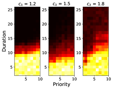
(a) True positives

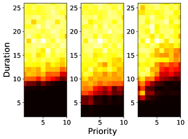
(b) False negatives

(c)

Figure 5: true positives and false negatives with $c_{\delta}=1.8$ and $\delta_{\mathrm{max}}=26$.

Meanwhile, $c_{\lambda}$ should be carefully tuned, otherwise it will lead to an undesired agent behavior. In Fig. 6, we retrain our environment for $c_{\delta}=30$ and, again, with increasing $c_{\lambda}$. We observe that agents trained with high values for $c_{\lambda}$ eventually start to prioritize false negatives (Eq. (5)). Hence, the results could be even worse than the baseline solution: lower acceptance rate (Fig. 6a) and higher false positive (Fig. 6b).

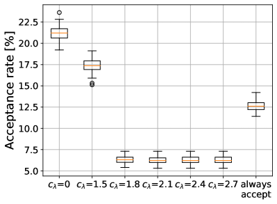
(a) Acceptance rate

(b) False negatives

Figure 6: Results of $c_{\lambda}$ parameter analysis with $c_{\delta}=1.8$ and $\delta_{\mathrm{max}}=30$

VI-C Changing maximum trained duration

In the previous sections, agents are trained with a fixed $\delta_{\mathrm{max}}$ and evaluated for different incoming $\delta_{\mathrm{max}}$. What if the agents were trained for a shorter $\delta_{\mathrm{max}}$? How would that impact the acceptance rate for incoming VNRs with longer, shorter, or equal to the trained $\delta_{\mathrm{max}}$?

To answer these questions, in total 9 agents are trained for $\delta_{\mathrm{max}}$ between 12 and 30 and evaluated, in addition to the baseline, for different $\delta_{\mathrm{max}}$ (Fig. 7). All training runs are performed with $c_{\delta}=1.8$, which is a compromise between increasing acceptance rate and limiting the number of false negatives as described in VI-A. We set $c_{\lambda}=0$.

In Fig. 7a, each agent shows the highest increase in median acceptance rate compared to the always accept baseline agent in the exact scenario it was trained for. For higher offered loads, the agents’ performance drops but still stays above the baseline level. This behavior results from agents not having encountered any larger VNR duration during training thus do not know how to properly deal with them during evaluation.

This can also be interpreted from Table II. Agents perform mostly the best when the trained and evaluated $\delta_{\mathrm{max}}$ are the same. As the difference between the trained and evaluated $\delta_{\mathrm{max}}$ increase, the acceptance rate decrease, but it is still better than the baseline solution. Meanwhile, Fig. 7b does not show consistent patterns for the relation between trained and evaluated $\delta_{\mathrm{max}}$ with respect to false negatives. Hence, it depends more on the environment and should be tuned with respect to other environment parameters (e.g., distribution of arriving VNR duration).

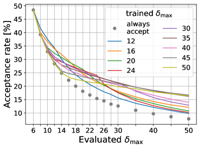
(a) Acceptance rate

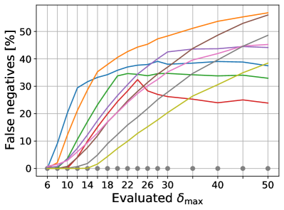
(b) False negatives

Figure 7: Impact of trained $\delta_{\mathrm{max}}$ on agent performance in different $\delta_{\mathrm{max}}$ enviromnets

TABLE II: Comparison between agents with different trained $\delta_{\mathrm{max}}$ in multiple $\delta_{\mathrm{max}}$ environments

eval $\delta_{\mathrm{max}}$	12	16	20	24	30	35	40	45	50
trained $\delta_{\mathrm{max}}$
12	34.3	26.8	22.3	19.2	15.6	13.6	12.1	10.9	9.8
16	33.9	29.5	24.7	21.5	18.1	16.0	14.3	13.0	12.1
20	32.2	29.1	26.3	22.0	17.7	15.3	13.5	12.0	10.8
24	30.2	27.9	25.9	24.1	17.5	14.6	12.7	11.3	10.2
30	30.9	27.7	25.5	23.7	21.2	18.1	15.8	14.1	12.9
35	29.9	26.9	25.1	23.5	21.3	19.6	18.3	17.1	16.2
40	30.3	26.0	24.0	22.4	20.4	18.4	16.6	15.1	14.0
45	28.8	24.7	23.5	22.6	20.9	19.6	18.5	17.5	16.7
50	28.4	23.3	22.1	21.2	19.8	19.0	17.9	17.1	16.4
baseline	28.4	22.2	18.1	15.4	12.6	11.0	9.7	8.6	7.8

VII Summary

This paper uses RL for admission control of VNRs in wireless VNE. RL agents are trained to maximize the revenue (e.g., acceptance rate or number prioritized VNR) by rejecting some VNRs to be able to accept more/better future VNRs. The agent’s behavior can be tuned by modifying the parameters $c_{\delta}$ and $c_{\lambda}$. On the one hand, low values of $c_{\delta}$ lead to a behavior with little to no increase in overall acceptance rate while keeping the number of false negatives small. High values of $c_{\delta}$ yield more false negatives aggressively, resulting in a higher overall acceptance rate, but with a diminishing return. On the other hand, the higher $c_{\lambda}$ the more likely the agent consider priority over duration. Hence, longer VNRs with a high priority value can be accepted. This should be carefully tuned, otherwise the results can be even worse than a first fit greedy baseline. Meanwhile, training an agent with a predefined $\delta_{\mathrm{max}}$ yields a better solution than the first fit baseline, even if there is a mismatch between the trained and deployed/evaluated $\delta_{\mathrm{max}}$.

References

- [1] Juliver Gil Herrera and Juan Felipe Botero. Resource allocation in nfv: A comprehensive survey. IEEE Transactions on Network and Service Management, 13(3):518–532, 2016.
- [2] Sevil Dräxler, Manuel Peuster, Marvin Illian, and Holger Karl. Generating resource and performance models for service function chains: The video streaming case. In 2018 4th IEEE Conference on Network Softwarization and Workshops (NetSoft), pages 318–322, 2018.
- [3] D. Praveen Kumar, Tarachand Amgoth, and Chandra Sekhara Rao Annavarapu. Machine learning algorithms for wireless sensor networks: A survey. Information Fusion, 49:1–25, 2019.
- [4] Ibrahim Mustapha, Borhanuddin M. Ali, A. Sali, M.F.A. Rasid, and H. Mohamad. An energy efficient reinforcement learning based cooperative channel sensing for cognitive radio sensor networks. Pervasive and Mobile Computing, 35:165–184, 2017.
- [5] H. Chen, X. Li, and F. Zhao. A reinforcement learning-based sleep scheduling algorithm for desired area coverage in solar-powered wireless sensor networks. IEEE Sensors Journal, 16(8):2763–2774, 2016.
- [6] Asif Hasnain and Holger Karl. Learning coflow admissions. In IEEE INFOCOM 2021 - IEEE Conference on Computer Communications Workshops (INFOCOM WKSHPS). IEEE Communications Society.
- [7] T.C.-K. Hui and Chen-Khong Tham. Adaptive provisioning of differentiated services networks based on reinforcement learning. IEEE Transactions on Systems, Man, and Cybernetics, Part C (Applications and Reviews), 33(4):492–501, 2003.
- [8] Penghao Sun, Zehua Guo, Sen Liu, Julong Lan, and Yuxiang Hu. Qos-aware flow control for power-efficient data center networks with deep reinforcement learning. In ICASSP 2020 - 2020 IEEE International Conference on Acoustics, Speech and Signal Processing (ICASSP), pages 3552–3556, 2020.
- [9] Xianfu Chen, Honggang Zhang, Celimuge Wu, Shiwen Mao, Yusheng Ji, and Medhi Bennis. Optimized computation offloading performance in virtual edge computing systems via deep reinforcement learning. IEEE Internet of Things Journal, 6(3):4005–4018, 2019.
- [10] Ying He, Nan Zhao, and Hongxi Yin. Integrated networking, caching, and computing for connected vehicles: A deep reinforcement learning approach. IEEE Transactions on Vehicular Technology, 67(1):44–55, 2018.
- [11] Timothy X. Brown, Hui Tong, and Satinder Singh. Optimizing admission control while ensuring quality of service in multimedia networks via reinforcement learning. In Proceedings of the 11th International Conference on Neural Information Processing Systems, NIPS’98, page 982–988, Cambridge, MA, USA, 1998. MIT Press.
- [12] Majid Raeis, Ali Tizghadam, and Alberto Leon-Garcia. Reinforcement learning-based admission control in delay-sensitive service systems. CoRR, abs/2008.09590, 2020.
- [13] Bai Liu, Qiaomin Xie, and Eytan Modiano. Reinforcement learning for optimal control of queueing systems. In 2019 57th Annual Allerton Conference on Communication, Control, and Computing (Allerton), pages 663–670, 2019.
- [14] Nguyen Cong Luong, Dinh Thai Hoang, Shimin Gong, Dusit Niyato, Ping Wang, Ying-Chang Liang, and Dong In Kim. Applications of deep reinforcement learning in communications and networking: A survey. IEEE Communications Surveys Tutorials, 21(4):3133–3174, 2019.
- [15] Pinyarash Pinyoanuntapong, Minwoo Lee, and Pu Wang. Delay-optimal traffic engineering through multi-agent reinforcement learning. In IEEE INFOCOM 2019 - IEEE Conference on Computer Communications Workshops (INFOCOM WKSHPS), pages 435–442, 2019.
- [16] A. Blenk, P. Kalmbach, P. van der Smagt, and W. Kellerer. Boost online virtual network embedding: Using neural networks for admission control. In 2016 12th International Conference on Network and Service Management (CNSM), pages 10–18, 2016.
- [17] Victor Millnert, Johan Eker, and Enrico Bini. Achieving predictable and low end-to-end latency for a network of smart services. In 2018 IEEE Global Communications Conference (GLOBECOM), pages 1–7, 2018.
- [18] Haipeng Yao, Sihan Ma, Jingjing Wang, Peiying Zhang, Chunxiao Jiang, and Song Guo. A continuous-decision virtual network embedding scheme relying on reinforcement learning. IEEE Transactions on Network and Service Management, 17(2):864–875, 2020.
- [19] A. Blenk, P. Kalmbach, J. Zerwas, M. Jarschel, S. Schmid, and W. Kellerer. Neurovine: A neural preprocessor for your virtual network embedding algorithm. In IEEE INFOCOM 2018 - IEEE Conference on Computer Communications, pages 405–413, 2018.
- [20] H. Afifi, S. Auroux, and H. Karl. Marvelo: Wireless virtual network embedding for overlay graphs with loops. In 2018 IEEE Wireless Communications and Networking Conference (WCNC), pages 1–6, 2018.
- [21] Gabriel Dulac-Arnold, Richard Evans, Peter Sunehag, and Ben Coppin. Reinforcement learning in large discrete action spaces. CoRR, abs/1512.07679, 2015.
- [22] Haitham Afifi and Holger Karl. An approximate power control algorithm for a multi-cast wireless virtual network embedding. In 2019 12th IFIP Wireless and Mobile Networking Conference (WMNC), pages 95–102, 2019.