Spatial Ensemble: a Novel Model Smoothing Mechanism for Student-Teacher Framework

Abstract

Model smoothing is of central importance for obtaining a reliable teacher model in the student-teacher framework, where the teacher generates surrogate supervision signals to train the student. A popular model smoothing method is the Temporal Moving Average (TMA), which continuously averages the teacher parameters with the up-to-date student parameters. In this paper, we propose “Spatial Ensemble”, a novel model smoothing mechanism in parallel with TMA. Spatial Ensemble randomly picks up a small fragment of the student model to directly replace the corresponding fragment of the teacher model. Consequentially, it stitches different fragments of historical student models into a unity, yielding the “Spatial Ensemble” effect. Spatial Ensemble obtains comparable student-teacher learning performance by itself and demonstrates valuable complementarity with temporal moving average. Their integration, named Spatial-Temporal Smoothing, brings general (sometimes significant) improvement to the student-teacher learning framework on a variety of state-of-the-art methods. For example, based on the self-supervised method BYOL, it yields $+0.9\%$ top-1 accuracy improvement on ImageNet, while based on the semi-supervised approach FixMatch, it increases the top-1 accuracy by around $+6\%$ on CIFAR-10 when only few training labels are available. Codes and models are available at: https://github.com/tengteng95/Spatial_Ensemble.

1 Introduction

Recent years have witnessed the success of the student-teacher framework in self-supervised [1, 2, 3, 4, 5] and semi-supervised [6, 7, 8] learning tasks. In this framework, the teacher is responsible for generating surrogate supervision signals to guide the learning of the student on unlabeled data, for example, category IDs for classification, feature patterns for contrastive learning, etc.

Many important works under this framework share a common model smoothing technique, i.e., the Temporal Moving Average (TMA), to generate the teacher from the student model. For example, Mean Teacher [6] for semi-supervision averages historical student weights as the teacher. MoCo [1] for self-supervision employs a slowly progressing encoder (teacher), driven by a momentum update with the query encoder (student). Another state-of-the-art method for self-supervision BYOL [2] employs a similar strategy to update the target (teacher) network with a slow-moving average of the online (student) network. We thus recognize that model smoothing with TMA is of central importance for obtaining a reliable teacher for these works.

In this paper, we rethink the mechanism of TMA and summarize its importance as two-fold. First, TMA enables the teacher to absorb parameters from different student editions and thus benefits from the model ensemble. Second, TMA constrains the variance of the teachers to be small to avoid inconsistent labels produced during two adjacent updates. An abrupt change to the pseudo labels will cripple training and possibly leads to optimization divergence. This is particularly important for self-supervised learning where annotations are unavailable.

We propose a novel model smoothing mechanism named “Spatial Ensemble”. Compared with TMA, Spatial Ensemble facilitates similar model smoothing benefits with a different mechanism, as illustrated in Figure 1. In TMA, the teacher absorbs each historical student as a whole. A temporally near student is absorbed into the teacher with a larger weighting factor due to the Exponential Moving Average effect. In contrast, in Spatial Ensemble, the teacher randomly picks up one or more small fragments of the student to replace the corresponding fragments of the teacher during each update. All the fragments are weighted equally in the teacher model. In this way, Spatial Ensemble stitches different fragments of previous student models into a unity, yielding the “Spatial Ensemble” effect. In spite of their fundamental differences, Spatial Ensemble facilitates similar benefits of model ensemble and smoothed update. The smoothed update is maintained by replacing only a small portion of parameters at each iteration. On the challenging self-supervised learning task, which is very sensitive to the quality of surrogate supervision signals, we observe that Spatial Ensemble achieves comparable performance with temporal moving average. It shows that our Spatial Ensemble can serve as a basic model smoothing technique for the student-teacher framework.

An important advantage of Spatial Ensemble lays in its complementarity to Temporal Moving Average. To explore their complementary benefits, we integrate both the temporal smoothing and spatial smoothing mechanism into a unified method named Spatial-Temporal Smoothing (STS). STS does not directly absorb a whole student, or simply replace a fragment. Instead, it updates a fragment of the teacher model with a temporal moving average of the corresponding fragment of the student. This “mix-up” model smoothing benefits from the mutual complementarity of temporal moving average and Spatial Ensemble. Experiments on both self-supervised and semi-supervised tasks show that using STS for model smoothing obtains general (sometimes significant) improvement over a majority of state-of-the-art methods.

We summarize our contribution as follows:
1. We propose a novel model smoothing mechanism named Spatial Ensemble. Compared with the popular temporal moving average, Spatial Ensemble achieves a comparable model smoothing effect with a different mechanism.

2. We integrate the spatial and temporal smoothing mechanism into a unified method named Spatial-Temporal Smoothing. STS benefits from the mutual complementarity of two mechanisms and consistently improves student-teacher methods on self- and semi-supervised learning tasks.

3. We notice two recognizable advantages of the model learned through STS, including strong robustness against various data corruptions, and superior transferring capability to the object detection task.

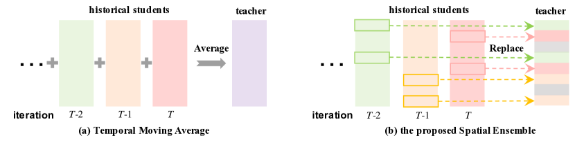
Figure 1: Illustration of Temporal Moving Average and Spatial Ensemble.

2 Related Work

In this section, we present a brief review of the development on semi- and self-supervised learning, as well as the student-teacher framework. We mainly focus on the recent deep learning literature related to our method.

Semi-supervised learning aims at achieving comparable performance to fully supervised methods, usually with a small portion of labeled data and the rest as unlabeled data. It is of great importance for real scenarios where annotations are difficult/expensive to acquire, such as medical data. Pseudo labels [9, 10] and consistency regularization [11, 7, 6] are two essential techniques in many recent semi-supervised approaches. Pseudo-Labeling [9] generates soft pseudo labels for the unlabeled data using the logits predicted by the model from the latest epoch. Laine et al. [10] improve the pseudo label generation process by leveraging a temporal ensembling prediction of different epochs. Mean-teacher [6] further simplifies this process by introducing a teacher model, which is a temporal ensembling of the student model through the exponential moving average, to generate pseudo labels directly. Besides, mean-teacher employs a consistency regularization to encourage similar predictions from the teacher and the student model. FixMatch [7] assumes that the consistency should also hold between images applied with augmentations of different degrees, and applies both a weak and a strong set of data augmentations.

Self-supervised learning largely narrows down its performance gap with supervised approaches and is receiving increasing attention in the community. Recent self-supervised methods can be roughly categorized into two genres, i.e., approaches based on pretext task and approaches based on contrastive learning. There are many kinds of insightful pretext task designs. One common method is generating surrogate supervision signals by feature clustering [12, 13, 14], image augmentation (usually rotation [15]), relative order of clipped image patches [16, 17, 18], etc. Another mainstream approach is to design a generative pretext task, e.g., image colorization [19, 20], image inpainting [21] and image denoising [22], and usually employ auto-encoders or generative adversarial networks [23] to transfer images. Instead of designing a pretext task, contrastive learning approaches [1, 4, 24, 25, 26, 27, 28, 29] aim at maximizing the feature similarities with augmented views produced from the identical image sample, while minimizing those from different image samples.

Student-teacher framework is a popular architecture that has been extensively used in many recent state-of-the-art methods, especially for semi- and self-supervised learning tasks. Usually, temporal moving average is employed to generate the teacher from historical student models. The optimization goal is to ensure the prediction consistency between the student and the teacher. Besides pulling different views of the same image closer, MoCo [1] employs a memory bank to store negative samples and pushes views from different images apart. BYOL [2] removes negative samples and leverages an asymmetric student-teacher architecture to prevent collapsing. An extra predictor is appended to the online (student) network to regress the output of the target (teacher) network.

3 Method

Preliminaries. Given a same network architecture, $\Theta^{\mathcal{T}}$ and $\Theta^{\mathcal{S}}$ are the parameters of the teacher and student model. Both $\Theta^{\mathcal{T}}$ and $\Theta^{\mathcal{S}}$ contains $n$ units of parameters, i.e., $\Theta^{\mathcal{T}}=\{\theta_{1}^{\mathcal{T}},\theta_{2}^{\mathcal{T}},\cdots,\theta_{n}^{\mathcal{T}}\}$ and $\Theta^{\mathcal{S}}=\{\theta_{1}^{\mathcal{S}},\theta_{2}^{\mathcal{S}},\cdots,\theta_{n}^{\mathcal{S}}\}$. A unit may correspond to a layer, a neuron or a channel, depending on the desired spatial granularity. To analyze the model update in consecutive iterations, we further define them as functions of the iteration $t$, i.e., $\Theta^{\mathcal{T}}(t)=\{\theta_{i}^{\mathcal{T}}(t)\}$ and $\Theta^{\mathcal{S}}(t)=\{\theta_{i}^{\mathcal{S}}(t)\}$.

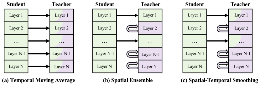
Figure 2: Illustration of three different model smoothing approaches TMA, SE, and STS.

3.1 Spatial Ensemble

We present a new model smoothing method named Spatial Ensemble (SE), as illustrated in Figure 2 (b). During each iteration, SE randomly picks up some units of the student model to replace the corresponding units of the teacher model, leaving the remaining parts of the teacher unchanged. We formulate this process as:

$$\Theta^{\mathcal{T}}(t)=\{\mathcal{P}_{i}\theta_{i}^{\mathcal{T}}(t-1)+(1-\mathcal{P}_{i})\theta_{i}^{\mathcal{S}}(t-1)\},$$ (1)

where $\mathcal{P}_{i}\sim Ber(p)$ (i.e., the Bernoulli distribution with success probability $p$) is a binary variable. We note that all $\mathcal{P}_{i}\sim Ber(p)(i=1,2,\cdots,n)$ are mutually independent to each other and have the same success probability $p$. It determines whether the $i$-th unit of the teacher parameters is to be preserved. Specifically, if $\mathcal{P}_{i}=1$, the $i$-th unit parameters is to be preserved. If $\mathcal{P}_{i}=0$, the $i$-th unit is to be replaced. Since $\mathcal{P}_{i}\sim Ber(p)$, larger $p$ results in lower replacing frequency and higher proportion of preserved units. Therefore, we name $p$ as the “preserving probability”.

For clarity, we omit the iteration indicator in all the equations in the following part of this paper and rewrite Equation 1 as:

$$\Theta^{\mathcal{T}}\Longleftarrow\{\mathcal{P}_{i}\theta_{i}^{\mathcal{T}}+(1-\mathcal{P}_{i})\theta_{i}^{\mathcal{S}}\}.$$ (2)

To investigate the mechanism of SE, we quantitatively analyze the smoothing effect on both the model parameters and the generated surrogate supervision signals. Specifically, we calculate the Mean-Square Errors (MSE) between teachers at two adjacent epochs, as well as the MSE between their outputs. We visualize the MSE values at the early training stages (epoch 1 to 20) in Fig. 3, from which we make two observations:

Remark 1: Spatial Ensemble smooths the teacher update. It is observed that without model smoothing, the MSE of both model parameters and supervision signals maintain relatively high values, indicating strong vibration during the teacher update. In another word, the teacher model and its output signals undergo substantial instability. In contrast, when using the TMA and the proposed SE to update the teacher, the MSE of both model parameters and supervision signals are much smaller (than Non-smoothing), yielding a smoothed teacher update.

Remark 2: Spatial Ensemble promotes convergence. Using TMA and SE, the MSE values gradually decrease as the training epochs increases. Such resulr indicates that the up-to-date teacher model gradually become closer to it prior edition, therefore approaching convergence. Without TMA or SE, the Non-smoothing mode maintains a roughly constant MSE value. We thus infer that Spatial Ensemble (as well as the TMA) promotes convergence of student-teacher framework.

We provide the pseudocode of SE in Algorithm 1, which is easy to implement with only a few lines of code. In Section 4.3, we further analyze the effect of $p$ on student-teacher learning performance.

Algorithm 1 Pseudocode of SE.

⬇

# net_s, net_t: student/teacher network

# m: momentum for TMA

# p: probability of a student layer belonging to the unpicked fragment.

params_s = net_s.parameters()

params_t = net_t.parameters()

for s, t in zip(params_s, params_t):

if random.rand() < p:

continue

else:

t = s

Algorithm 2 Pseudo code of STS.

⬇

# net_s, net_t: student/teacher network

# m: momentum for TMA

# p: probability of a student layer belonging to the unpicked fragment.

params_s = net_s.parameters()

params_t = net_t.parameters()

for s, t in zip(params_s, params_t):

if random.rand() < p:

continue

else:

t = m * t + (1-m) * s

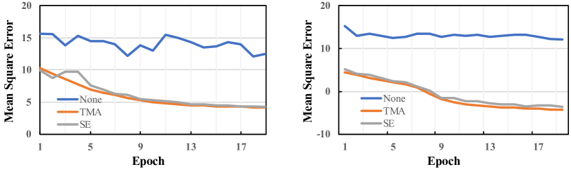
Figure 3: Illustration of mean square error of teacher parameters (Left) and generated supervision signals (Right) at two adjacent epochs. None represents no model smoothing is used. TMA adopts a momentum of 0.999. $p$ is set to 0.999 for SE. The vertical coordinates are arranged in Log scales.

3.2 Spatial-Temporal Smoothing

We further integrate TMA and SE into a unified model smoothing method named Spatial-Temporal Smoothing (STS), to benefit from their mutual complementarity. STS picks up several units in the student model and averages them with the corresponding units in the teacher model, which is formulated as:

$$\Theta^{\mathcal{T}}\Longleftarrow\{\mathcal{P}_{i}\theta_{i}^{\mathcal{T}}+(1-\mathcal{P}_{i})m\theta_{i}^{\mathcal{T}}+(1-\mathcal{P}_{i})(1-m)\theta_{i}^{\mathcal{S}}\},$$ (3)

where $m$ is the momentum for TMA.

STS degenerates to SE or TMA, given specification of hyper-parameters. When $m=0$, STS degenerates into SE. Similarly, when we set the preserving probability $p=1$, which results in $\mathcal{P}_{i}\equiv 0$, STS degenerates into TMA:

$$\Theta^{\mathcal{T}}\Longleftarrow m\Theta^{\mathcal{T}}+(1-m)\Theta^{\mathcal{S}},$$ (4)

Algorithm 2 illustrates the pseudocode of STS. Similar to SE, STS is easy to implement and can be integrated into most teacher-student frameworks. In Section 4.3, we present detailed analysis of how $p$ and $m$ influence the performance of STS.

4 Experiments

4.1 Baselines and Implementation Details

We evaluate the effectiveness of the proposed Spatial-Temporal Smoothing by applying it to the state-of-the-art self-supervised approaches (MoCo [1] and BYOL [2]) and semi-supervised method (FixMatch [7]). We use the official implementation of MoCo and re-implement BYOL and FixMatch using Pytorch [30]. All experiments are conducted on a machine with 8 RTX2080 GPUs. The masking probability $p$ is set to 0.7/0.5/0.5 for BYOL/MoCo/FixMatch, respectively. We dump the teacher model at the end of training. The self-supervised models are evaluated by following the common protocol of linear classification [4, 31, 2, 1] while semi-supervised performance are assessed with top-1 accuracy metric. We carefully follow both the training and evaluation settings of  [1, 2, 7] in their original paper for fair comparison. More details are given in the following.

MoCo [1] consists of a query model and a key model, which simulates the same role as the student and the teacher model, respectively. We adopt MoCo v2 with ResNet-50 as our baseline and use a memory bank of size 65536. The initial learning rate is set to 0.03 and adjusted by cosine learning rate scheduler [32]. Following the original paper, we train the model using SGD with momentum of 0.9, weight decay of 0.0001, and a mini-batchsize of 256. Both the query and key model adopt the same data augmentations as SimCLR [4], i.e., random crop, horizontal flip, color jitter, Gaussian blur, and gray-scale conversion.

BYOL [2] reformulates the self-supervised learning task as a regression task which maximizes the similarity of feature representations from the teacher and the student model. We train BYOL with Synchronized batch normalization [33] and use a mini-batchsize of 256. The basic learning rate is 0.1 and is decayed by cosine strategy [32]. The first 10 epochs are warmed up with a factor of 0.001 and gradually increased to the basic learning rate. We adopt SGD with momentum of 0.9 as the optimizer and set weight decay to 1e-4. BYOL uses the same set of data augmentations as SimCLR [4] as listed above, and adopts solarization with probability of 0.2 for the teacher model.

FixMatch [7] uses identical student and teacher network in the training phase while employing the TMA teacher for evaluation. We use Wide ResNet-28-2 [34] and Wide ResNet-28-8 as the backbone networks for CIFAR-10 and CIFAR-100, respectively. We use SGD with momentum 0.9 as the optimizer and train the model for $2^{20}$ iterations following the original paper. Each mini-batch comprises of 64 labeled images and 448 unlabeled images (i.e., 1:7). The initial learning rate is 0.03 and is decayed by cosine scheduler [32]. The weight decay is set to 0.0005 and 0.001 for CIFAR-10 and CIFAR-100, respectively. For data augmentation, the student only uses random crop and random horizontal flip. Besides these two augmentations, the teacher additionally adopts random augmentation [35].

Evaluation. Linear Evaluation is a common metric for measuring whether the feature representation learned by the self-supervised model is good. Typically, a classifier is appended to the feature encoder and finetuned on the down-streaming task. During the whole process, the parameters of the feature encoder, as well as the BN statistics, are fixed. We train the classifier appended to MoCo using the SGD optimizer for 100 epochs. The initial learning rate is 30 and is decayed at the 60th and 80th epoch with factor 0.1. For BYOL, the basic learning rate is 0.2 and is adjusted according to the cosine strategy during the full 80 epochs.

4.2 The Effect of SE and STS

We first evaluate the effect of SE on the self-supervised task. We select MoCo and BYOL as the baseline models and train them for 200 epochs. As shown in Table 1, disabling the model smoothing mechanism in MoCo and BYOL leads to failure of convergence, which is also observed in their original papers. The experimental results indicate the importance of model smoothing in these self-supervised approaches. When combined with SE, MoCo/BYOL achieves 66.7%/67.8% top-1 accuracy, demonstrating the effectiveness of SE in model smoothing.

We further validate the effectiveness of STS which integrates both the temporal and spatial smoothing strategies. As is shown in Table 2, compared to typical TMA, our method boosts the performance of MoCo (BYOL) from 67.5% (71.8%) to 67.8% (72.7%) in terms of top-1 accuracy, indicating the valuable complementarity of the spatial and temporal smoothing mechanism.

Method	Smoothing	top-1	top-5
MoCo	-	fail	fail
MoCo	SE	66.7	87.0
BYOL	-	fail	fail
BYOL	SE	67.8	88.3

Table 1: Analysis of the effectiveness of SE as a model smoothing approach.

Method	Smoothing	top-1	top-5
MoCo	TMA	67.5	88.0
MoCo	STS	67.8	88.1
BYOL	TMA	71.8	90.6
BYOL	STS	72.7	90.9

Table 2: Analysis of the superiority of STS over TMA.

4.3 Ablation Studies

In this section, we evaluate the effect of hyperparameters in STS and then investigate Spatial Ensemble of different granularities. BYOL is adopted as the default network for the following experiments. All the ablation experiments are conducted on the ImageNet dataset [36] and trained for 200 epochs unless noted otherwise.

Effect of hyperparameters $p$ and $m$. To explore how $p$ and $m$ influences the student-teacher learning performance, we conduct extensive experiments by selecting $m$ from {0, 0.9, 0.99, 0.999} and varying $p$ 0.1 to 0.9 with an interval of 0.2. We first investigate the effect of $p$ by setting $m=0$. Under this case, STS degenerates into SE. As is shown in Figure 4, BYOL fails to converge when $p=0$ while achieves increasing performance with the increase of $p$, demonstrating the importance of model smoothing. Figure 4 illustrates the results with different combinations of $p$ and $m$. It can be observed that STS yields better performance than typical TMA ($p=0$) in most cases. We also notice an interesting fact that with the increase (decrease) of $m$, the model achieves its best performance at relatively smaller (larger) value of $p$. For example, $p=0.99$ is the best choice when $m$ is set to 0.9. However, for $m=0.99$, a smaller $p$ of 0.7 yields much better performance than larger $p$ of 0.99. These results demonstrate the complementarity of spatial and temporal smoothing, as well as the important role of model smoothing for self-supervised learning based on the student-teacher framework.

Granularity of Spatial Ensemble. SE may have various granularities, corresponding to a layer, a channel, or a neuron as the smallest unit. When integrating SE into STS, we set the granularity to layer-wise by default. In this section, we investigate the impacts of different granularities, i.e., layer-wise (LW), channel-wise (CW) and neuron-wise (NW). Specifically, for a student parameter with shape $C_{in}\times C_{out}$, where $C_{in}$ and $C_{out}$ denote the number of input and output channels, respectively. For CW, we randomly pick up a small set of indexes along with the $C_{out}$ dimension and replace the corresponding teacher parameters. Similarly for NW, we randomly select neurons from the whole student model and replace the corresponding neurons of the teacher model. As shown in the top of Table 4, SE using NW outperforms its counterpart using LW and CW and achieves comparable performance with TMA. The result reveals that SE itself benefits from the fine-grained spatial ensemble. Besides, three variants of STS result in comparable performance, indicating the complementarity of temporal smoothing and spatial ensemble. When combined with temporal smoothing, LW is capable to produce a representative teacher model as good as its fine-grained counterpart NW. Considering that the time cost of LW is lower than both CW and NW, yet their performances are close, we use LW as default.

4.4 Self-supervised evaluation of STS

In this part, we substitute the model smoothing mechanism in BYOL [2] with our STS and compare the resulted model to other state-of-the-art methods on self-supervised learning. Furthermore, we investigate the robustness of our method to corrupted data. Finally, we evaluate the transfer capability of our method on the object detection task.

Comparison with State-of-the-art method. Table 3 presents the linear evaluation results of our method compared with the state-of-the-art self-supervised method on ImageNet [36]. Using BYOL as the base model, STS yields competitive top-1 accuracies of 73.0% and 74.5% under 300 and 1000 epochs, outperforming previous state-of-the-art approaches. It is worth noting that our model is trained with a smaller batch size of 256, while BYOL requires 4096. According to the results in the original BYOL paper, when the batch size decreases from 4096 to 256, its top-1 accuracy drops around than 0.6%.

Robust to corruptions on ImageNet-C. We further evaluate the robustness of our method to data corruptions. Specifically, we select ImageNet-C [37], which is a standard benchmark dataset for evaluating the model robustness to common corruptions and perturbations, as our testbed. There are 15 different corruption types in ImageNet-C. Besides, each type has 5 corrpution intensities. In the left part of Figure 5, we give some image examples of corruptions from ImageNet-C and the corresponding top-1 accuracy improvements of STS over TMA. Combining the right part of Figure 5, we observe that STS outperforms TMA under all the five corruption intensity settings and yields an improvement of around 1.5% in terms of the mean top-1 accuracy of 75 corruption combinations. Besides, considering a single corruption from these 75 combinations, STS leads to an improvement of around 0.5% $\sim$ 5.6%. These results demonstrate the superiority of our method in terms of the robustness to corruptions and further reveal the advantage of STS in enhancing the representative capability of the teacher model.

Transfer learning in object detection. We further evaluate the generalization ability of the learned representation using our approach for the more challenging object detection task. In Table 5, we compare our method with state-of-the-art self-supervised approaches. All the self-supervised models are trained for 200 epochs on the ImageNet dataset and then finetuned with the joint split of VOC2007 trainval and VOC2012 train. And their results are taken from SimSiam [38]. For fair comparison, we carefully follow the training and evaluation settings in SimSiam [38]. In more detail, we use the same detection codebase as SimSiam [38] and MoCo [1]. The default detector is Faster-RCNN [39] with a backbone of R50-C4. We finetune all the layers and BN statistics for 24,000 iterations with 16 images per batch. The image scales is set to [480, 800] pixels in the traning stage while 800 for inference. The initial learning rate is 0.02 and is decreased by a factor of 0.1 and 0.01 at when reaching 18,000 and 22,000 iterations. We can observe from Table 5 that the representation learned by our approach can be well transferred to downstream detection task and achieves comparable or superior performance than previous approaches, especially on the AP₇₅ metric.

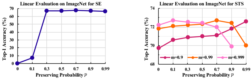
Figure 4: Linear evaluation results of SE (Left) and STS (Right) under different hyperparameter settings.

Method	Epoch	top-1	top-5
Jigsaw [40]	90	45.7	-
InstDis [41]	200	56.5	-
BigBiGAN [42]	-	56.5	-
Local Agg. [43]	-	60.2	-
CPC v2 [25]	200	63.8	85.3
SimCLR [4]	200	66.6	-
MoCo v2 [1]	200	67.5	-
PCL [44]	200	67.6	-
InfoMin Aug [24]	200	70.1	89.4
Swav [3]	400	70.7	-
SimSiam [38]	400	70.8	-
BYOL [2]	300	72.5	90.8
Ours (BYOL + STS)	300	73.0	91.3
PIRL [45]	800	63.6	-
SimCLR [4]	1000	69.3	89.0
InfoMin Aug [24]	800	73.0	91.1
MoCo v2 [1]	800	71.1	-
SimSiam [38]	800	71.3	-
Swav [3]	800	71.8	-
BYOL [2]	1000	74.3	91.6
Ours (BYOL + STS)	1000	74.5	91.8

Table 3: Comparison with state-of-the-art self-supervised methods on ImageNet under linear evaluation. All the experiments are based on ResNet-50 and pretrained with two $224\times 224$ views without multi-crop augmentation.

Method	Smoothing	top-1	time
TMA	-	71.8	$1.0\times$
SE	LW	67.8	$0.97\times$
SE	CW	70.8	$1.02\times$
SE	NW	71.6	$1.80\times$
STS	LW	72.7	$0.99\times$
STS	CW	72.8	$1.04\times$
STS	NW	72.8	$1.82\times$

Table 4: Comparison of SE and STS with different granularities.

pretrain	VOC07+12 detection
	AP50	AP	AP75
supervised	81.3	53.5	58.8
SimCLR	81.8	55.5	58.8
MoCo v2	82.3	57.0	63.3
SwAV	81.5	55.4	61.4
SimSiam	82.4	57.0	63.7
BYOL	81.4	55.3	61.1
Ours	82.3	57.2	64.4

Table 5: Transfer learning on VOC object detection benmark.

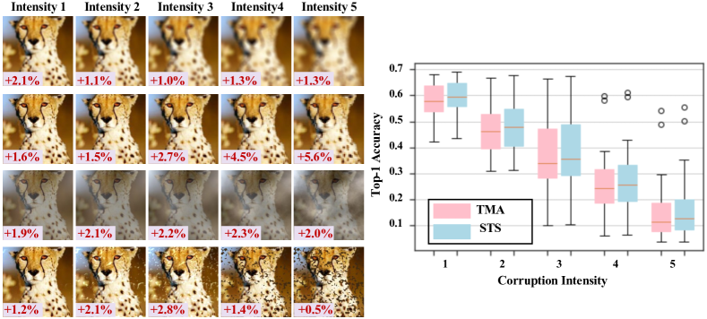
Figure 5: Left: Examples of 4 corruption types, namely defocus blur, pixelate, fog, and spatter. The numbers attached to the left-bottom corner denote the improvement of STS over TMA on the corresponding corruption type and intensity in terms of top-1 accuracy. Right: Comparison of top-1 accuracy between TMA and STS on ImageNet-C.

Method	CIFAR-10				CIFAR-100
	20 labels	40 labels	250 labels	4000 labels	200 labels	400 labels	2500 labels	10000 labels
$\prod$-Model [46]	-	-	45.74	85.99	-	-	42.75	62.12
Pseudo-Labeling [9]	-	-	50.22	83.91	-	-	42.62	63.79
Mean Teacher [6]	-	-	67.68	90.81	-	-	46.09	64.17
MixMatch [47]	-	52.46	88.95	93.58	-	32.39	60.06	71.69
UDA [48]	-	70.95	81.18	95.12	-	40.72	66.87	75.50
ReMixMatch [49]	-	80.90	94.56	95.28	-	55.72	72.57	76.97
FixMatch	86.68	92.06	94.89	95.77	42.78	52.54	70.75	76.53
FixMatch (STS)	93.31	93.89	95.10	95.94	45.85	55.25	72.22	77.92

Table 6: Comparison with state-of-the-art semi-supervised methods on the CIFAR-10 and CIFAR-100 benchmark datasets under the top-1 accuracy metric.

4.5 Semi-supervised Evaluation of STS

This part is to evaluate the performance of our STS when integrated with FixMatch [7] for semi-supervised learning. Following the common settings [6, 7], we use CIFAR-10 and CiFAR-100 as the benchmark datasets.

CIFAR-10. We evaluate our method on CIFAR-10 under four settings, i.e., using 2, 4, 25, 400 labels per class. As shown in Table 6, STS achieves consistently superior performance than TMA under these four different settings, yielding an improvement of 6.63%, 1.83%, 0.21%, and 0.17%, respectively. Although the numerical improvement is relatively small when 250/4000 labels are available, it is actually non-trivial since the results have already been very close to the performance upper bound (97.01%), which leverages all labels of 50,000 CIFAR-10 images. The comparison with 20/40 labels is more valuable since how to narrow the performance gap between semi-supervised and supervised learning with limited annotations is a heated research topic in the community. The remarkable improvement achieved by STS demonstrate its superiority and indicates the potential practical value in real scenarios where usually few labeled data is available.

CIFAR-100. In Table 6, we further provide the results on CIFAR-100 benchmark dataset under four settings, i.e., using 2, 4, 25, and 100 labels per class. Similar to the phenomenon observed in CIFAR-10, STS achieves noticeable improvements when only a few labels (200/400 labels) are given, outperforming the baseline by 3.07% and 2.71%. Besides, with more labels (2500/10000 labels), STS also achieves consistent improvements of 1.47% and 1.39%, demonstrating the effectiveness of our approach.

5 Conclusion

This paper reveals a new mechanism for model smoothing from the spatial ensemble perspective. In addition to the capacity of model smoothing, an important advantage of spatial ensemble is its complementarity to the popular temporal moving average. To benefit from such complementarity, we integrate temporal moving average and spatial ensemble into a unified model smoothing method named Spatial-Temporal Smoothing (STS). Extensive experiments on self-supervised and semi-supervised tasks show that STS brings general improvement to many state-of-the-art methods. Besides, STS achieves competitive results on the ImageNet-C dataset and the downstream object detection task, demonstrating its good generalization ability.

References

- He et al. [2020] Kaiming He, Haoqi Fan, Yuxin Wu, Saining Xie, and Ross B. Girshick. Momentum contrast for unsupervised visual representation learning. In Proc. of IEEE Intl. Conf. on Computer Vision and Pattern Recognition, 2020.
- Grill et al. [2020] Jean-Bastien Grill, Florian Strub, Florent Altché, Corentin Tallec, Pierre H. Richemond, Elena Buchatskaya, Carl Doersch, Bernardo Ávila Pires, Zhaohan Guo, Mohammad Gheshlaghi Azar, Bilal Piot, Koray Kavukcuoglu, Rémi Munos, and Michal Valko. Bootstrap your own latent - A new approach to self-supervised learning. In Proc. of Advances in Neural Information Processing Systems, 2020.
- Caron et al. [2020a] Mathilde Caron, Ishan Misra, Julien Mairal, Priya Goyal, Piotr Bojanowski, and Armand Joulin. Unsupervised learning of visual features by contrasting cluster assignments. In Proc. of Advances in Neural Information Processing Systems, 2020a.
- Chen et al. [2020a] Ting Chen, Simon Kornblith, Mohammad Norouzi, and Geoffrey E. Hinton. A simple framework for contrastive learning of visual representations. In Proc. of Intl. Conf. on Machine Learning, 2020a.
- Zbontar et al. [2021] Jure Zbontar, Li Jing, Ishan Misra, Yann LeCun, and Stéphane Deny. Barlow twins: Self-supervised learning via redundancy reduction. CoRR, 2021.
- Tarvainen and Valpola [2017] Antti Tarvainen and Harri Valpola. Mean teachers are better role models: Weight-averaged consistency targets improve semi-supervised deep learning results. In Proc. of Advances in Neural Information Processing Systems, 2017.
- Sohn et al. [2020] Kihyuk Sohn, David Berthelot, Nicholas Carlini, Zizhao Zhang, Han Zhang, Colin Raffel, Ekin Dogus Cubuk, Alexey Kurakin, and Chun-Liang Li. Fixmatch: Simplifying semi-supervised learning with consistency and confidence. In Proc. of Advances in Neural Information Processing Systems, 2020.
- Arazo et al. [2020] Eric Arazo, Diego Ortego, Paul Albert, Noel E. O’Connor, and Kevin McGuinness. Pseudo-labeling and confirmation bias in deep semi-supervised learning. In Proc. of International Joint Conference on Neural Networks, 2020.
- Lee et al. [2013] Dong-Hyun Lee et al. Pseudo-label: The simple and efficient semi-supervised learning method for deep neural networks. In Proc. of Intl. Conf. on Machine Learning Workshop, 2013.
- Laine and Aila [2017] Samuli Laine and Timo Aila. Temporal ensembling for semi-supervised learning. In 5th International Conference on Learning Representations, ICLR 2017, Toulon, France, April 24-26, 2017, Conference Track Proceedings. OpenReview.net, 2017. URL https://openreview.net/forum?id=BJ6oOfqge.
- Miyato et al. [2019] Takeru Miyato, Shin-ichi Maeda, Masanori Koyama, and Shin Ishii. Virtual adversarial training: A regularization method for supervised and semi-supervised learning. IEEE Trans. Pattern Anal. Mach. Intell., 41:1979–1993, 2019.
- Caron et al. [2018] Mathilde Caron, Piotr Bojanowski, Armand Joulin, and Matthijs Douze. Deep clustering for unsupervised learning of visual features. In Proc. of European Conference on Computer Vision, 2018.
- Caron et al. [2019] Mathilde Caron, Piotr Bojanowski, Julien Mairal, and Armand Joulin. Unsupervised pre-training of image features on non-curated data. In Porc. of IEEE Intl. Conf. on Computer Vision, 2019.
- Caron et al. [2020b] Mathilde Caron, Ishan Misra, Julien Mairal, Priya Goyal, Piotr Bojanowski, and Armand Joulin. Unsupervised learning of visual features by contrasting cluster assignments. In Proc. of Advances in Neural Information Processing Systems, 2020b.
- Gidaris et al. [2018] Spyros Gidaris, Praveer Singh, and Nikos Komodakis. Unsupervised representation learning by predicting image rotations. In Proc. of International Conference on Learning Representations, 2018.
- Noroozi and Favaro [2016a] Mehdi Noroozi and Paolo Favaro. Unsupervised learning of visual representations by solving jigsaw puzzles. In Proc. of European Conference on Computer Vision, 2016a.
- Doersch et al. [2015] Carl Doersch, Abhinav Gupta, and Alexei A. Efros. Unsupervised visual representation learning by context prediction. In Porc. of IEEE Intl. Conf. on Computer Vision, 2015.
- Doersch and Zisserman [2017] Carl Doersch and Andrew Zisserman. Multi-task self-supervised visual learning. In Porc. of IEEE Intl. Conf. on Computer Vision, 2017.
- Zhang et al. [2016] Richard Zhang, Phillip Isola, and Alexei A. Efros. Colorful image colorization. In Proc. of European Conference on Computer Vision, 2016.
- Zhang et al. [2017] Richard Zhang, Phillip Isola, and Alexei A. Efros. Split-brain autoencoders: Unsupervised learning by cross-channel prediction. In Proc. of IEEE Intl. Conf. on Computer Vision and Pattern Recognition, 2017.
- Pathak et al. [2016] Deepak Pathak, Philipp Krähenbühl, Jeff Donahue, Trevor Darrell, and Alexei A. Efros. Context encoders: Feature learning by inpainting. In Proc. of IEEE Intl. Conf. on Computer Vision and Pattern Recognition, 2016.
- Vincent et al. [2008] Pascal Vincent, Hugo Larochelle, Yoshua Bengio, and Pierre-Antoine Manzagol. Extracting and composing robust features with denoising autoencoders. In Proc. of Intl. Conf. on Machine Learning, 2008.
- Goodfellow et al. [2014] Ian J Goodfellow, Jean Pouget-Abadie, Mehdi Mirza, Bing Xu, David Warde-Farley, Sherjil Ozair, Aaron Courville, and Yoshua Bengio. Generative adversarial networks. Proc. of Advances in Neural Information Processing Systems, 2014.
- Tian et al. [2020a] Yonglong Tian, Chen Sun, Ben Poole, Dilip Krishnan, Cordelia Schmid, and Phillip Isola. What makes for good views for contrastive learning? In Proc. of Advances in Neural Information Processing Systems, 2020a.
- Hénaff [2020] Olivier J. Hénaff. Data-efficient image recognition with contrastive predictive coding. In Proc. of Intl. Conf. on Machine Learning, 2020.
- Bachman et al. [2019] Philip Bachman, R. Devon Hjelm, and William Buchwalter. Learning representations by maximizing mutual information across views. In Proc. of Advances in Neural Information Processing Systems, 2019.
- Hjelm et al. [2019] R. Devon Hjelm, Alex Fedorov, Samuel Lavoie-Marchildon, Karan Grewal, Philip Bachman, Adam Trischler, and Yoshua Bengio. Learning deep representations by mutual information estimation and maximization. In Proc. of International Conference on Learning Representations, 2019.
- Tian et al. [2020b] Yonglong Tian, Dilip Krishnan, and Phillip Isola. Contrastive multiview coding. In Proc. of European Conference on Computer Vision, 2020b.
- Misra and van der Maaten [2020a] Ishan Misra and Laurens van der Maaten. Self-supervised learning of pretext-invariant representations. In Proc. of IEEE Intl. Conf. on Computer Vision and Pattern Recognition, 2020a.
- Paszke et al. [2019] Adam Paszke, Sam Gross, Francisco Massa, Adam Lerer, James Bradbury, Gregory Chanan, Trevor Killeen, Zeming Lin, Natalia Gimelshein, Luca Antiga, Alban Desmaison, Andreas Köpf, Edward Yang, Zachary DeVito, Martin Raison, Alykhan Tejani, Sasank Chilamkurthy, Benoit Steiner, Lu Fang, Junjie Bai, and Soumith Chintala. Pytorch: An imperative style, high-performance deep learning library. In Proc. of Advances in Neural Information Processing Systems, 2019.
- Chen et al. [2020b] Ting Chen, Simon Kornblith, Kevin Swersky, Mohammad Norouzi, and Geoffrey E. Hinton. Big self-supervised models are strong semi-supervised learners. In Proc. of Advances in Neural Information Processing Systems, 2020b.
- Loshchilov and Hutter [2017] Ilya Loshchilov and Frank Hutter. SGDR: stochastic gradient descent with warm restarts. In Proc. of International Conference on Learning Representations, 2017.
- Peng et al. [2018] Chao Peng, Tete Xiao, Zeming Li, Yuning Jiang, Xiangyu Zhang, Kai Jia, Gang Yu, and Jian Sun. Megdet: A large mini-batch object detector. In Proc. of IEEE Intl. Conf. on Computer Vision and Pattern Recognition, 2018.
- Zagoruyko and Komodakis [2016] Sergey Zagoruyko and Nikos Komodakis. Wide residual networks. In Proc. of British Machine Vision Conference, 2016.
- Cubuk et al. [2020] Ekin Dogus Cubuk, Barret Zoph, Jon Shlens, and Quoc Le. Randaugment: Practical automated data augmentation with a reduced search space. In Proc. of Advances in Neural Information Processing Systems, 2020.
- Russakovsky et al. [2015] Olga Russakovsky, Jia Deng, Hao Su, Jonathan Krause, Sanjeev Satheesh, Sean Ma, Zhiheng Huang, Andrej Karpathy, Aditya Khosla, Michael S. Bernstein, Alexander C. Berg, and Fei-Fei Li. Imagenet large scale visual recognition challenge. International Journal of Computer Vision, pages 211–252, 2015.
- Hendrycks and Dietterich [2019] Dan Hendrycks and Thomas G. Dietterich. Benchmarking neural network robustness to common corruptions and perturbations. In Proc. of International Conference on Learning Representations, 2019.
- Chen and He [2020] Xinlei Chen and Kaiming He. Exploring simple siamese representation learning. CoRR, 2020.
- Ren et al. [2015] Shaoqing Ren, Kaiming He, Ross B. Girshick, and Jian Sun. Faster R-CNN: towards real-time object detection with region proposal networks. In Proc. of Advances in Neural Information Processing Systems, 2015.
- Noroozi and Favaro [2016b] Mehdi Noroozi and Paolo Favaro. Unsupervised learning of visual representations by solving jigsaw puzzles. In Proc. of European Conference on Computer Vision, 2016b.
- Wu et al. [2018] Zhirong Wu, Yuanjun Xiong, Stella X. Yu, and Dahua Lin. Unsupervised feature learning via non-parametric instance discrimination. In Proc. of IEEE Intl. Conf. on Computer Vision and Pattern Recognition, 2018.
- Donahue and Simonyan [2019] Jeff Donahue and Karen Simonyan. Large scale adversarial representation learning. In Proc. of Advances in Neural Information Processing Systems, 2019.
- Zhuang et al. [2019] Chengxu Zhuang, Alex Lin Zhai, and Daniel Yamins. Local aggregation for unsupervised learning of visual embeddings. In Porc. of IEEE Intl. Conf. on Computer Vision, 2019.
- Li et al. [2020] Junnan Li, Pan Zhou, Caiming Xiong, Richard Socher, and Steven C. H. Hoi. Prototypical contrastive learning of unsupervised representations. CoRR, 2020.
- Misra and van der Maaten [2020b] Ishan Misra and Laurens van der Maaten. Self-supervised learning of pretext-invariant representations. In Proc. of IEEE Intl. Conf. on Computer Vision and Pattern Recognition, 2020b.
- Rasmus et al. [2015] Antti Rasmus, Mathias Berglund, Mikko Honkala, Harri Valpola, and Tapani Raiko. Semi-supervised learning with ladder networks. In Proc. of Advances in Neural Information Processing Systems, 2015.
- Berthelot et al. [2019] David Berthelot, Nicholas Carlini, Ian J. Goodfellow, Nicolas Papernot, Avital Oliver, and Colin Raffel. Mixmatch: A holistic approach to semi-supervised learning. In Proc. of Advances in Neural Information Processing Systems, 2019.
- Xie et al. [2020] Qizhe Xie, Zihang Dai, Eduard H. Hovy, Thang Luong, and Quoc Le. Unsupervised data augmentation for consistency training. In Proc. of Advances in Neural Information Processing Systems, 2020.
- Berthelot et al. [2020] David Berthelot, Nicholas Carlini, Ekin D. Cubuk, Alex Kurakin, Kihyuk Sohn, Han Zhang, and Colin Raffel. Remixmatch: Semi-supervised learning with distribution matching and augmentation anchoring. In Proc. of International Conference on Learning Representations, 2020.