Minimal theory of massive gravity and constraints on the graviton mass

Abstract

The Minimal theory of Massive Gravity (MTMG) is endowed non-linearly with only two tensor modes in the gravity sector which acquire a non-zero mass. On a homogeneous and isotropic background the theory is known to possess two branches: the self-accelerating branch with a phenomenology in cosmology which, except for the mass of the tensor modes, exactly matches the one of $\Lambda$CDM; and the normal branch which instead shows deviation from General Relativity in terms of both background and linear perturbations dynamics. For the latter branch we study using several early and late times data sets the constraints on today’s value of the graviton mass $\mu_{0}$, finding that $(\mu_{0}/H_{0})^{2}=0.119_{-0.098}^{+0.12}$ at 68% CL, which in turn gives an upper bound at 95% CL as $\mu_{0}<8.4\times 10^{-34}$ eV. This corresponds to the strongest bound on the mass of the graviton for the normal branch of MTMG.

I Introduction

These years have shown several unexpected results from the experimental side [1, 2, 3, 4, 5]. Probably the most important one is the discovery of gravitational waves [6]. These modes are indeed showing the tensorial nature of the ripples of the spacetime, as correctly predicted by Einstein. This new discovery led in turn to a revolution also into the research of the predictions made by several theoretical models to the speed of propagation of gravitational waves [7]. In particular, the fact that we have seen two neutron stars merging with each other, gave us the chance to probe the speed of propagation for such waves compared to the one of electromagnetic waves together with the possibility of determining $H_{0}$ [8, 9]. The measurement gave strong constraints on the propagation of gravitational waves. Although the measurement was regarding small redshifts ($z<0.05$), nonetheless the gravitational waves had to be traveling through non trivial backgrounds (the wave had to travel at least the spacetime around the source, the one of the galaxy to which the source belongs, the inter-galactic region between the source-galaxy and the Milky Way, and finally the spacetime of our galaxy and the one of our solar system, see e.g. [10]. This kinematical observable pin-pointed the speed of propagation for such waves very close to the speed of light. In fact, several scalar tensor theories have been ruled out as predicting a speed of propagation which significantly differs today from unity [11].

As a matter of fact, the discovery of the gravitational waves led necessarily to the search for another fundamental property of theirs: what is the value of the mass appearing in the dispersion relation for such spacetime ripples? In order to be consistent with the multi-messenger measurement discussed above, the mass cannot be too large as this would change the speed of propagation considerably [12, 13]. General Relativity (and many other theories too) predicts that the tensor modes are massless. This is indeed consistent with the usual picture of gravity being a force with an infinite range. However, without assuming any theoretical prior, we could be addressing, just using any data at hand, the issue of determining the value of the mass for gravitational waves.

Although this phenomenological approach is well motivated, still one would find it more convincing if, after all, there exists a sensible theory which allows for a non-zero value for the mass of gravitational waves. If not, even the point of searching would look a bit philosophical, or at most, it would be an approach which is still incomplete as waiting for a good theory to be proposed. Fortunately, a theory which allows for a non-zero mass for the tensorial gravitational waves and at the same time which is not immediately ruled out by either theoretical or experimental constraints does exist [14]. This theory, the minimal theory of massive gravity (MTMG), is a modification of the massive gravity theory introduced in [15] (dRGT). Compared to dRGT, MTMG introduces a modification by breaking 4D Lorentz-invariance and removing through appropriate non-linear constraints the (three) modes which otherwise make the cosmological solutions of dRGT unstable/strongly coupled [16].

MTMG (as well as dRGT) allows for the existence of two different branches, namely: 1) the self-accelerating branch and 2) the normal branch. The self-accelerating branch shows exactly the same phenomenology as $\Lambda$CDM both at the level of the homogeneous and isotropic background and at the level of linear perturbation theory for scalar and vector modes [17]. The only difference is the presence of a mass for the tensor modes which does not modify the linear growth of structures. This branch then shares the same set of observational/experimental constraints with $\Lambda$CDM.

The normal branch of MTMG is a different beast. It gives a phenomenology of linear scalar perturbation which is different from $\Lambda$CDM so that it can give rise to new and interesting constraints from the data [18, 19]. On top of that, without introducing any new propagating degrees of freedom, the normal branch of MTMG allows the presence of a dynamical dark energy component, and such a dynamics can be set by appropriately choosing the fiducial metric to match essentially any desired profile. Recently the simplest possible dynamics for the normal branch (that reproduces the background dynamics of $\Lambda$CDM) has been studied in [20] and led to the surprising feature that the Planck data tend to set the squared mass of the tensor modes, $\mu^{2}$, to be a positive quantity (at 1-sigma). In fact, although this result was consistent with late time data only, still the data were allowing a large region of $\mu^{2}<0$ (i.e. the graviton could be a ultralight tachyonic field).

In this work, we seek constraints on the graviton mass in the presence of a background dynamical component that is intrinsically and generically present in the normal branch of MTMG. We will introduce five additional new parameters (compared to $\Lambda$CDM) for the model, but as we will see later on, joining all the chosen data sets will provide very strong constraints on the (time-dependent) mass of graviton. In particular we find that in MTMG, the considered data sets (to be described in more detail in the following, including Planck 2018) do not show internal tensions and all together lead to a bound on today’s value for the mass of the graviton as $\mu_{0}^{2}=2.5{}_{-4.8}^{+4.5}\times 10^{-67}\ {\rm eV}^{2}$. As far as we know, this result is the strongest constraint we have on the mass of the graviton for the normal branch of MTMG.

II The theory

The theory we want to discuss here is the minimal theory of massive gravity, MTMG. This theory has been constructed as to have only two degrees of freedom (the gravitational waves) in the gravity sector and as to share the same background dynamics as dRGT. In order to achieve these goals we adopt the usual ADM formalism and consider the physical lapse function $N$, the physical shift vector $N^{i}$ and the physical three dimensional metric $\gamma_{ij}$ as basic variables. We also need to choose a fiducial lapse function and a fiducial three dimensional metric which in the unitary gauge corresponds to given external fields

$$M\,,\quad\tilde{\gamma}_{ij}\,,$$ (1)

together with another three dimensional external field $\tilde{\zeta}^{i}{}_{j}$, which is related to the rate of change of the vielbein forming $\tilde{\gamma}_{ij}$. (In the following sections these three external fields will be chosen to be functions of time only, as to be able to have a homogeneous description of our universe at large scales.)

We can then introduce the tensor $\mathcal{K}^{i}{}_{j}$ defined by

$$\mathcal{K}^{i}{}_{l}\mathcal{K}^{l}{}_{j}=\tilde{\gamma}^{il}\gamma_{lj}\,,$$ (2)

where $\tilde{\gamma}^{il}$ is the inverse of $\tilde{\gamma}_{ij}$, that is $\tilde{\gamma}^{il}\tilde{\gamma}_{lj}=\delta^{i}{}_{j}$. Then we can also introduce the inverse tensor $\mathfrak{K}^{i}{}_{j}$ of $\mathcal{K}^{i}{}_{j}$, defined as

$$\mathfrak{K}^{i}{}_{l}\mathcal{K}^{l}{}_{j}=\delta^{i}{}_{j}=\mathcal{K}^{i}{}_{l}\,\mathfrak{K}^{l}{}_{j}\,.$$ (3)

Out of these building blocks we can introduce a symmetric 2-tensor (in three dimensions) as

$$\Theta^{ij}=\frac{\sqrt{\tilde{\gamma}}}{\sqrt{\gamma}}\,\{c_{1}\,(\gamma^{il}\mathcal{K}^{j}{}_{l}+\gamma^{jl}\mathcal{K}^{i}{}_{l})+c_{2}\,[\mathcal{K}\,(\gamma^{il}\mathcal{K}^{j}{}_{l}+\gamma^{jl}\mathcal{K}^{i}{}_{l})-2\tilde{\gamma}^{ij}]\}+2c_{3}\,\gamma^{ij}\,,$$ (4)

where $\tilde{\gamma}$ and $\gamma$ are the determinants of $\tilde{\gamma}_{ij}$ and $\gamma_{ij}$ respectively, whereas $\mathcal{K}\equiv\mathcal{K}^{l}{}_{l}$. Hereafter, $c_{\mu}$ ($\mu\in\{1,\dots,4\}$) are free numerical constants. As usual, we can introduce the extrinsic curvature tensor $K_{ij}$ defined as

$$K_{ij}=\frac{1}{2N}\,(\dot{\gamma}_{ij}-D_{i}N_{j}-D_{j}N_{i})\,,$$ (5)

where $D_{i}$ is the three dimensional covariant derivative compatible with $\gamma_{ij}$, that is $D_{m}\gamma_{ij}=0$. Now, we can define a three dimensional scalar $\mathcal{C}_{0}$ as

$$\mathcal{C}_{0}=\frac{1}{2}\,m^{2}\,M\,K_{ij}\,\Theta^{ij}-m^{2}M\left\{\frac{\sqrt{\tilde{\gamma}}}{\sqrt{\gamma}}\,\{c_{1}\,\tilde{\zeta}+c_{2}\,[(\mathcal{K}\tilde{\zeta}-\mathcal{K}^{i}{}_{l}\tilde{\zeta}^{l}{}_{i})]+c_{3}\,\mathfrak{K}^{i}{}_{l}\tilde{\zeta}^{l}{}_{i}\right\},$$ (6)

where $m$ is a mass-dimension scale (related to the graviton mass), and we have also named $\tilde{\zeta}\equiv\tilde{\zeta}^{l}{}_{l}$. It is also necessary to introduce the following three dimensional 2-tensor $\mathcal{C}^{i}{}_{j}$ as

$$\mathcal{C}^{i}{}_{j}=-m^{2}M\left\{\frac{\sqrt{\tilde{\gamma}}}{\sqrt{\gamma}}\,\bigl{[}\tfrac{1}{2}\,(c_{1}+c_{2}\mathcal{K})\,(\mathcal{K}^{i}{}_{j}+\gamma^{il}\mathcal{K}^{m}{}_{l}\gamma_{mj})-c_{2}\,\tilde{\gamma}^{il}\gamma_{lj}\bigr{]}+c_{3}\,\delta^{i}{}_{j}\right\}.$$ (7)

We can then introduce the action for MTMG as

$$S=S_{{\rm pre}}+\frac{M_{\rm P}^{2}}{2}\int d^{4}xN\sqrt{\gamma}\left(\frac{m^{2}}{4}\,\frac{M}{N}\,\lambda\right)^{2}\bigl{(}\Theta_{ij}\Theta^{ij}-\tfrac{1}{2}\,\Theta^{2}\bigr{)}-\frac{M_{\rm P}^{2}}{2}\int d^{4}x\sqrt{\gamma}\left[\lambda\mathcal{C}_{0}+(D_{i}\lambda^{j})\mathcal{C}^{i}{}_{j}\right]+S_{{\rm mat}}\,,$$ (8)

where we have introduced a Lagrange multiplier $\lambda$ together with another three dimensional vector Lagrange multiplier $\lambda^{i}$. Furthermore we have defined $\Theta_{ij}\equiv\gamma_{im}\gamma_{jn}\Theta^{mn}$ and $\Theta\equiv\gamma_{ij}\Theta^{ij}$, and $S_{{\rm mat}}$ is the action for the standard matter fields minimally coupled to the four-dimensional metric made of the ADM variables ($N$, $N^{i}$, $\gamma_{ij}$). Finally, $S_{{\rm pre}}$ is given by

$$S_{{\rm pre}}\equiv S_{{\rm GR}}+\frac{M_{\rm P}^{2}}{2}\,\sum_{n=1}^{4}\int d^{4}x\,\mathcal{S}_{n}\,,$$ (9)

where

$$S_{{\rm GR}} = \frac{M_{\rm P}^{2}}{2}\int d^{4}x\,N\sqrt{\gamma}\,[{}^{(3)}R+K^{ij}K_{ij}-K^{2}]\,,$$ (10)

$$\mathcal{S}_{1} = -m^{2}c_{1}\sqrt{\tilde{\gamma}}\,(N+M\mathcal{K})\,,$$ (11)

$$\mathcal{S}_{2} = -\frac{1}{2}\,m^{2}\,c_{2}\sqrt{\tilde{\gamma}}\,(2N\mathcal{K}+M\mathcal{K}^{2}-M\tilde{\gamma}^{ij}\gamma_{ji})\,,$$ (12)

$$\mathcal{S}_{3} = -m^{2}\,c_{3}\sqrt{\gamma}\,(M+N\mathfrak{K})\,,$$ (13)

$$\mathcal{S}_{4} = -m^{2}\,c_{4}\sqrt{\gamma}\,N\,,$$ (14)

${}^{(3)}R$ is the Ricci scalar for the three dimensional metric $\gamma_{ij}$, $K^{ij}\equiv\gamma^{im}\gamma^{jn}K_{mn}$, $K\equiv\gamma^{ij}K_{ij}$, and $\mathfrak{K}\equiv\mathfrak{K}^{l}{}_{l}$.

III The cosmological background

The action (8) is the full action of the theory which can be studied on any desired background, as long as it is compatible with the equations of motion for the theory. In the following we will focus on a homogeneous and isotropic background, as to study the cosmology for this theory. First of all, let us fix the fiducial metric $\tilde{\gamma}_{ij}=\tilde{a}(t)^{2}\,\delta_{ij}$ (so that $\tilde{\gamma}^{ij}=\tilde{a}^{-2}\,\delta^{ij}$), and, at the same time, also the fiducial lapse $M=M(t)$, and the rate of change for the fiducial vielbein $\tilde{\zeta}^{i}{}_{j}=\frac{\dot{\tilde{a}}}{M\,\tilde{a}}\,\delta^{i}{}_{j}$. Notice that having adopted the unitary gauge these fiducial variables come as purely background quantities. From the viewpoint of the physical sector, these correspond to external fields which explicitly break Lorentz invariance at the cosmological scale.

As for the remaining variables we will first set up the physical lapse, shift and 3D metric as follows:

$$N = N(t)\,(1+\alpha)\,,$$ (15)

$$N_{i} = N(t)\,\partial_{i}\chi\,,$$ (16)

$$\gamma_{ij} = a(t)^{2}\,[\delta_{ij}(1+2\zeta)+2a^{-2}\partial_{i}\partial_{j}E]\,.$$ (17)

Here, we have set not only the background but also the linear perturbation variables, $\alpha,\chi,\zeta$, and $E$. Since we have imposed the unitary gauge to hold, we cannot impose any further gauge conditions on the perturbation variables. On the other hand, we still have a freedom to re-select an arbitrary monotonic function of the time coordinate for the background of the temporal Stückelberg field. As a result, we can freely set, if needed, $N(t)$ to a conveniently chosen positive function of time, e.g. $N(t)=1$ or $N(t)=a(t)$. (If we a priori fix $N(t)$ in this way then the background equations of motion determines $M(t)$ instead of $N(t)$. See (27) below.) Now we can find the solution to the equation $\mathcal{K}^{i}{}_{l}\mathcal{K}^{l}{}_{j}=\tilde{\gamma}^{il}\gamma_{lj}$, order by order in perturbations, giving the fact that at the lowest order (i.e. on the background) we have $\mathcal{K}^{i}{}_{j}=(a/\tilde{a})\,\delta^{i}{}_{j}=\delta^{i}{}_{j}/X$. Here, we have introduced the background variable $X=X(t)$ defined as $\tilde{a}=X\,a$. We are now able to write down $\mathcal{S}_{1}$, $\mathcal{S}_{2}$ and $\mathcal{S}_{4}$. Along the same line, on finding the inverse of $\mathcal{K}^{i}{}_{j}$, namely $\mathfrak{K}^{i}{}_{j}$, we can write down also $\mathcal{S}_{3}$. After introducing

$$\lambda = \lambda(t)+\delta\lambda\,,$$ (18)

$$\lambda^{i} = \frac{1}{a^{2}}\,\delta^{ij}\partial_{j}\delta\lambda_{f}\,,$$ (19)

we have all the remaining building blocks which form the full action of the theory. Here, we have focused our attention only to the background and scalar perturbation modes. As for the remaining ones, vector modes dynamics is the same as GR (see e.g. [17]), whereas the tensor modes will get a massive dispersion relation, which will be described, for our convenience, later on.

We can introduce the matter fields in the usual ADM formalism without fixing any gauge. Just to give an example we will write here a perfect fluid component (labeled with a variable $I$), whose Schutz-Sorkin action [21, 22] reads

$$S_{{\rm pf}}^{(I)}=-\int d^{4}x\sqrt{-g}[\rho_{I}(n_{I})+J_{I}^{\mu}\partial_{\mu}\varphi_{I}]\,.$$ (20)

Here, $n_{I}\equiv\sqrt{-J_{I}^{\mu}J_{I}^{\nu}g_{\mu\nu}}$, and $J_{I}^{\mu}$ form the components of a time-like four-vector, out of which we have the normalized 4-velocity of the fluid $u_{I}^{\mu}\equiv J_{I}^{\mu}/n$. Then we write

$$J_{I}^{0} = \frac{J_{I}^{0}(t)}{N(t)}\,(1+\delta j_{0}^{I})\,,$$ (21)

$$J_{I}^{i} = \frac{1}{a^{2}}\,\delta^{ij}\partial_{j}\delta j_{I}\,,$$ (22)

$$\varphi_{I} = \varphi_{I}(t)+\delta\varphi_{I}\,.$$ (23)

The background equations of motion for the fluid impose that $J_{I}^{0}(t)=\mathcal{N}_{I}/a^{3}$, where $\mathcal{N}_{I}={\rm constant}$, together with $\varphi_{I}=-\int^{t}N(t^{\prime})\,\frac{\partial\rho_{I}}{\partial n_{I}}\,dt^{\prime}$. Having fixed the matter fields, whose background equations of motion do not get any modification (after all we are only changing the gravity sector), we are ready to move on to the remaining modified Einstein equations and the additional constraints introduced in MTMG.

One property of MTMG is that on the cosmological background the equations of motion lead, as a unique solution, to $\lambda(t)=0$. In this case the modified Friedmann equation reads

$$3M_{\rm P}^{2}H^{2} = \rho_{X}+\sum_{I}\rho_{I}\,,$$ (24)

$$\rho_{X} \equiv \frac{1}{2}\,m^{2}M_{\rm P}^{2}\,(c_{1}X^{3}+3c_{2}X^{2}+3c_{1}X+c_{4})\,.$$ (25)

The constraint introduced in MTMG leads to the following equation of motion

$$\mathcal{E}_{\lambda}=(c_{1}X^{2}+2c_{2}X+c_{3})\left(\frac{\dot{X}}{N}+HX-H\,\frac{M}{N}\right)=0\,.$$ (26)

As in dRGT, the factorized structure of this equation allows for the presence of two distinct branches of solutions [23]. In particular the so-called self-accelerating branch, defined by setting the first factor to vanish, leads to a quadratic algebraic equation for $X$, which implies $X={\rm constant}$. As a consequence, on this branch $\rho_{X}={\rm constant}$, and the dynamics of the cosmological background is the same as the one for $\Lambda$CDM.

On the other hand, for the so-called normal branch we solve $\mathcal{E}_{\lambda}=0$ by setting the second factor in (26) to vanish. This in turn, assuming $H\neq 0$, leads to

$$M=\frac{\dot{X}}{H}+N\,X\,.$$ (27)

Since now on, we will consider this branch since the self-accelerating branch is indistinguishable from $\Lambda$CDM (even at the level of perturbations, as far as scalar and vector perturbations are concerned ). Notice that we have fixed $M(t)$ as in (27), but still $X(t)$ is free, because $\tilde{a}(t)$, the scale factor of the fiducial metric, has to be understood as a given function of time (or as a fixed function of the temporal Stückelberg field in the covariant formulation), that can be freely specified as a part of the definition of the theory.

We can rewrite then the modified second Einstein equation as

$$2M_{\rm P}^{2}\,\frac{\dot{H}}{N} = -\sum_{I}(\rho_{I}+P_{I})-(\rho_{X}+P_{X})\,,$$ (28)

$$\rho_{X}+P_{X} = -\frac{1}{2}\,m^{2}M_{\rm P}^{2}\,\frac{\dot{X}}{NX}\,(c_{1}X^{2}+2c_{2}X+c_{3})\,.$$ (29)

As a direct consequence of these equations, in the normal branch, in general we should expect a time-dependent, i.e. dynamical component $\rho_{X}$ whose dynamics can be given a priori. In other words, although in the gravity sector there are no propagating degrees of freedom beside the gravitational tensor modes, still the background has non-trivial dynamics, in general different from the one of $\Lambda$CDM. What we intend to do in the present paper is to find constraints on the mass of the graviton in the normal branch allowing non-trivial background dynamics for $X(t)$, or, equivalently, for $\rho_{X}$.

III.1 Background dynamics

Given the functional freedom of choosing $\rho_{X}$, we will consider the normal branch of MTMG with a background which deviates only slightly from the one of $\Lambda$CDM. In particular, let us consider a background which interpolates two $\Lambda$CDM’s with slightly different cosmological constants. This interpolation is defined by giving an explicit form for the Hubble expansion rate in terms of the redshift $z$ as follows

$$\frac{H^{2}}{H_{0}^{2}}=\frac{H_{\Lambda{\rm{CDM}}}^{2}(z)}{H_{0}^{2}}+\left[f(z)-1\right]\Delta+\mathcal{O}(\Delta^{2})\,,$$ (30)

where

$$\frac{H_{\Lambda{\rm{CDM}}}^{2}(z)}{H_{0}^{2}} = \Omega_{m0}(1+z)^{3}+\Omega_{r0}(1+z)^{4}+1-\Omega_{m0}-\Omega_{r0}\,,$$ (31)

$$f(z) = \frac{1+\tanh\frac{A_{2}-z}{A_{2}A_{3}}}{1+\tanh A_{3}^{-1}}\,.$$ (32)

This form was motivated by a recent work in the context of minimally modified gravity [24]. The exact $\Lambda$CDM limit takes place when $\Delta\to 0$. Also notice that at low redshifts $0\leq z\ll A_{2}$, we have $\left[f(z)-1\right]\Delta\to 0$ and thus $H\simeq H_{\Lambda{\rm{CDM}}}(z)$. On the other hand, when $z\gg A_{2}$ (high redshifts), then

$$\frac{H^{2}}{H_{0}^{2}}=\frac{H_{\Lambda{\rm{CDM}}}^{2}(z)}{H_{0}^{2}}-\Delta+\mathcal{O}(\Delta^{2})\,,$$ (33)

which corresponds to a shift of the cosmological constant (the sign of $\Delta$ will be fixed by the data).

The modified Friedmann equation of MTMG, in the presence of some radiation and dust components is written as

$$3M_{\rm P}^{2}H^{2}=\rho_{m}+\rho_{r}+\rho_{X}\,,$$ (34)

where $\rho_{X}$ is given by (25). Now, in order to realize the behavior of $H(z)$ shown in (30), let us consider $X$ of the form

$$X=X(z)=1+(A_{1}-1)\,f(z)\,,\quad f(z)=\frac{1+\tanh\frac{A_{2}-z}{A_{2}A_{3}}}{1+\tanh(A_{3}^{-1})}\,.$$ (35)

(The value of $\Delta$ will be given in terms of $A_{1}$ as shown in (49) below.) In this case $X$ will show a transition between two different constant values, namely from $X=1$ for large redshifts to $X=A_{1}$. Indeed, if we require that $A_{2}>0$ (for the MC sampling we assume $A_{2}>0.12$ for the reason that will be explained later) and that $0<A_{3}\ll 1$, then the transition happens in the past. As a result, $\rho_{X}$ will also interpolate two constants. Notice that this transition is smooth for both $X$ and $\rho_{X}$, taking place at around $z\approx A_{2}$. Then we have at all times

$$\frac{H^{2}}{H_{0}^{2}}=\Omega_{m0}(1+z)^{3}+\Omega_{r0}(1+z)^{4}+\frac{m^{2}}{6H_{0}^{2}}\,(c_{1}X^{3}+3c_{2}X^{2}+3c_{3}X+c_{4})\,,$$ (36)

as a given function of $z$. We can redefine the parameters of the theory as

$$\bar{c}_{\mu}=c_{\mu}\,\frac{m^{2}}{H_{0}^{2}}\,,\qquad\mu\in\{1,\dots,4\}\,,$$ (37)

so that

$$\frac{H^{2}}{H_{0}^{2}}=\Omega_{m0}(1+z)^{3}+\Omega_{r0}(1+z)^{4}+\frac{1}{6}\,(\bar{c}_{1}X^{3}+3\bar{c}_{2}X^{2}+3\bar{c}_{3}X+\bar{c}_{4})\,,$$ (38)

where $X$ is given by (35). In the following, we will make use of the following variables

$$\varrho_{I} \equiv \frac{\rho_{I}}{3M_{\rm P}^{2}}\,,\quad p_{I}\equiv\frac{P_{I}}{3M_{\rm P}^{2}}\,,$$ (39)

$$\varrho_{X} \equiv \frac{\rho_{X}}{3M_{\rm P}^{2}}=(H_{0}^{2}/6)\,(\bar{c}_{1}X^{3}+3\bar{c}_{2}X^{2}+3\bar{c}_{3}X+\bar{c}_{4})\,,$$ (40)

$$p_{X} \equiv \frac{P_{X}}{3M_{\rm P}^{2}}=-\frac{1}{3}\frac{H_{0}^{2}}{2}\,X(\bar{c}_{1}X^{2}+2\bar{c}_{2}X+\bar{c}_{3})\,\frac{\dot{X}}{NHX}-\varrho_{X}\,,$$ (41)

$$= -\frac{1}{3}\,H_{0}^{2}\,\theta\,\epsilon_{X}-\varrho_{X}\,,$$

$$\theta(t) \equiv \frac{1}{2}\,X(\bar{c}_{1}X^{2}+2\bar{c}_{2}X+\bar{c}_{3})\,,$$ (42)

$$\epsilon_{X} \equiv \frac{\dot{X}}{NHX}=-(1+z)\frac{1}{X}\,X_{,z}\,,$$ (43)

where $X_{,z}=dX/dz$. From the second Einstein equation we also find (28)-(29), which can be rewritten as

$$\frac{\dot{H}}{N}=-\frac{3}{2}(\varrho_{X}+p_{X})-\frac{3}{2}\,\sum_{I}(\varrho_{I}+p_{I})\,.$$ (44)

On defining

$$\Omega_{{\rm DE},0}\equiv 1-\Omega_{m0}-\Omega_{r0}\,,$$ (45)

we find that for $z=0$

$$\Omega_{{\rm DE},0}=\frac{1}{6}\,(\bar{c}_{1}A_{1}^{3}+3\bar{c}_{2}A_{1}^{2}+3\bar{c}_{3}A_{1}+\bar{c}_{4})\,,$$ (46)

which can be used to rewrite $\bar{c}_{4}$ as

$$\bar{c}_{4}=6\Omega_{{\rm DE},0}-(\bar{c}_{1}A_{1}^{3}+3\bar{c}_{2}A_{1}^{2}+3\bar{c}_{3}A_{1})\,.$$ (47)

On the other hand at high redshifts $X\approx 1$, we have $\rho_{X}\to{\rm constant}$ and thus matching (38) (with $X$ given by (35)) to (30) results in

$$\frac{1}{6}\,(\bar{c}_{1}+3\bar{c}_{2}+3\bar{c}_{3})+\frac{1}{6}\bar{c}_{4}=\Omega_{{\rm DE},0}-\Delta+\mathcal{O}(\Delta^{2})\,,$$ (48)

which can be used in order to write down $\Delta$ in terms of $A_{1}$ and $\bar{c}_{i}$ ($i\in\{1,2,3\}$) as

$$\Delta=\frac{1}{6}[\bar{c}_{1}(A_{1}^{3}-1)+3\bar{c}_{2}(A_{1}^{2}-1)+3\bar{c}_{3}(A_{1}-1)]\,.$$ (49)

This vanishes either when $A_{1}=1$ or when $\bar{c}_{i}\to 0$. In other words, the exact $\Lambda$CDM background is recovered by setting either $A_{1}=1$ or $\bar{c}_{i}=0$ ($i\in\{1,2,3\}$). We also have

$$\frac{M}{N}=\frac{\dot{X}}{HN}+X=-(1+z)\,X_{,z}+X\,,$$ (50)

and the squared mass of the graviton, as we shall see later on, reads

$$\mu^{2}=\frac{1}{2}\,m^{2}\,X\left[c_{2}X+c_{3}+\frac{M}{N}\,(c_{1}X+c_{2})\right].$$ (51)

If we assume that $A_{2}>0$ and $0<A_{3}\ll 1$, then around today we find, since $X_{,z}\approx 0$, that $M/N=X=A_{1}$ so that

$$\theta_{0}\equiv\frac{\mu_{0}^{2}}{H_{0}^{2}}=\frac{1}{2}\,A_{1}\,[\bar{c}_{1}A_{1}^{2}+2\bar{c}_{2}A_{1}+\bar{c}_{3}]\,,$$ (52)

which can be used to find today’s value of the mass of the graviton in terms of $A_{1}$ and $c_{i}$. In the $\Lambda$CDM limit this mass vanishes.

III.2 Independent model parameters

Then we choose $A_{1},A_{2},\Omega_{{\rm DE},0},\bar{c}_{i}$ ($i\in\{1,2,3\}$) as the independent free parameters to run MC sampling. In principle we could also count the parameter $A_{3}$ (which sets the speed of transition). However, we have checked that the bestfit to the data does not depend on $A_{3}$, so that we can safely fix it to a small value as $A_{3}=10^{-3}$. On top of these $5$ ($+1$) parameters we also have the standard matter parameters. Then, as already stated above, one can find the following derived parameters

$$\theta_{0} = \frac{1}{2}A_{1}^{3}\bar{c}_{1}+A_{1}^{2}\bar{c}_{2}+\frac{1}{2}A_{1}\bar{c}_{3}\,,$$ (53)

$$\Delta = \left(A_{1}^{3}-1\right)\frac{\bar{c}_{1}}{6}+\left(A_{1}^{2}-1\right)\frac{\bar{c}_{2}}{2}+\left(A_{1}-1\right)\frac{\bar{c}_{3}}{2}\,,$$ (54)

$$\bar{c}_{4} = -A_{1}^{3}\bar{c}_{1}-3A_{1}^{2}\bar{c}_{2}-3A_{1}\bar{c}_{3}+6\Omega_{{\rm DE},0}\,,$$ (55)

where

$$\Omega_{{\rm DE},0}\equiv 1-\Omega_{m0}-\Omega_{r0}\,.$$ (56)

It should be noted that $A_{1}>0$, because $X$ is required to be positive. Otherwise the fiducial metric would have a vanishing scale factor. Furthermore, in order to prevent a rapid change from taking place only around today, we assume $A_{2}$ to be larger than 0.12. Flat priors with a sufficiently wide range are instead given to the $\bar{c}_{i}$ parameters.

IV Cosmological Perturbations

Let us first define all the perturbation variables which enter in the theory, keeping in mind we have already fixed a gauge for the perturbations, namely the unitary gauge. This study has been already performed in [20], and thus we will only summarize here the results. In any case, the equations of motion to be inserted in the Boltzmann solver appear here, as far as we know, for the first time in the literature. Since the vector perturbations dynamics have been shown to be exactly equal to the $\Lambda$CDM case, we will not mention them in the following. Instead, as usual, the scalar sector needs to be explained in more detail.

We have already introduced the variables up to first order in perturbation theory in the scalar sector. In the following we will find it useful to consider the following definitions

$$\eta_{X}(t) \equiv \bar{c}_{2}X(t)^{2}+\bar{c}_{3}X(t)+\frac{1}{2}\theta(t)^{2}Y(t)-2\theta(t)\,,\qquad Y(t)\equiv\frac{H_{0}^{2}}{H^{2}}\,,$$ (57)

$$\Gamma = \sum_{I}\Gamma_{I}\,,\qquad\Gamma_{I}=\varrho_{I}+p_{I}\,.$$ (58)

We can now expand up to second order the total action, including the total matter Lagrangian. One can introduce a phenomenological description of matter by starting with Lagrangians for perfect fluids and then adding to them the shear perturbation terms as done in [24]. For the Schutz-Sorkin action for perfect fluids, already introduced above, we have $u_{Ii}=J_{Ii}/n_{I}=g_{i\alpha}J_{I}^{\alpha}/n_{I}$. This leads to

$$\delta j_{I}=\frac{\mathcal{N}_{I}}{a^{3}}\,(v_{I}-\chi)\,,$$ (59)

where we have defined $u_{Ii}=\partial_{i}v_{I}$. Through this field redefinition, we have now introduced a field which has a simple physical meaning. The equation of motion for $\delta j_{I}$ can now be used in order to set the following constraint

$$\delta\varphi_{I}=\rho_{I,n}\,v_{I}\,,$$ (60)

which eliminates fields in the matter sector. By expanding the quantity $\rho_{I}/\rho_{I}(t)-1$ up to first order of perturbations, and calling such a variable $\delta\rho_{I}/\rho_{I}$, then we have that

$$\delta j_{0}^{I}=\frac{\rho_{I}}{n_{I}\rho_{I,n}}\,\frac{\delta\rho_{I}}{\rho_{I}}-\alpha\,.$$ (61)

This equation can be used as a field redefinition introducing the fields $\delta\rho_{I}/\rho_{I}$ in the matter sector, which have a clear physical meaning.

At this level we can find the equations of motion for all the perturbations we have in the gravity and matter sectors. For instance, by “$\mathcal{E}_{\alpha}$” we will name the equation of motion obtained by taking variation of the second order action with respect to the field $\alpha$. In this case we have the following equations of motion: $\mathcal{E}_{\alpha}$, $\mathcal{E}_{\chi}$, $\mathcal{E}_{\zeta}$, $\mathcal{E}_{E}$, $\mathcal{E}_{\delta\lambda}$, $\mathcal{E}_{\delta\lambda_{f}}$, $\mathcal{E}_{\delta\rho_{I}/\rho_{I}}$, $\mathcal{E}_{v_{I}}$. Each of these expression is required to vanish, being the equations of motion for the perturbations.

We can now set $N(t)=a(t)$ on the background, but we cannot choose any gauge fixing for the perturbation fields since we have already adopted the unitary gauge. Nonetheless, since Lorentz violation is introduced only in the gravity sector at cosmological scales and the percolation of the Lorentz violation to the matter sector due to graviton loops is suppressed by negative powers of $M_{\rm P}^{2}$, any quantities that can be observed by any probes made of matter fields should be (either exactly or approximately) gauge-invariant in the sense of the four-dimensional diffeomorphism. Therefore it is useful to define gauge invariant perturbation variables as follows

$$\alpha = \psi-\frac{1}{a}\,\dot{\chi}+\frac{1}{a}\,\partial_{t}\!\left[a\partial_{t}\!\left(\frac{E}{a^{2}}\right)\right],$$ (62)

$$\zeta = -\phi-H\,\chi+aH\,\partial_{t}\!\left(\frac{E}{a^{2}}\right),$$ (63)

$$\frac{\delta\rho_{I}}{\rho_{I}} = \delta_{I}-\frac{\dot{\rho}_{I}}{a\rho_{I}}\,\chi+\frac{\dot{\rho}_{I}}{\rho_{I}}\,\partial_{t}\!\left(\frac{E}{a^{2}}\right),$$ (64)

$$v_{I} = -\frac{a}{k^{2}}\,\theta_{I}+\chi-a\,\partial_{t}\!\left(\frac{E}{a^{2}}\right).$$ (65)

These gauge invariant variables, namely $\psi$, $\phi$, $\delta_{I}$, $\theta_{I}$ are nothing but the gauge invariant variables which define the longitudinal-gauge variables, including the Bardeen potentials [25]. Here $\theta$ with index $I$ represents the field associated with matter velocity and is a perturbation variable. The index $I$ refers for fluid components like, radiation $r$, cold dark matter $c$, etc. It is different from $\theta$ that appeared in the background variable associated with the pressure from the minimal massive gravity (42).

As for the matter equations of motion, they exactly reduce to the $\Lambda$CDM case, namely

$$\dot{\delta}_{I} = -3aH(c_{sI}^{2}-w_{I})\,\delta_{\mathrm{I}}-(1+w_{I})\,\theta_{I}+3(1+w_{I})\,\dot{\phi}\,,$$ (66)

$$\dot{\theta}_{I} = aH(3c_{sI}^{2}-1)\,\theta_{I}+k^{2}\psi+\frac{c_{sI}^{2}k^{2}}{1+w_{I}}\,\delta_{I}-k^{2}\sigma_{I}\,,$$ (67)

where $c_{sI}^{2}=(\partial p_{I}/\partial\rho_{I})_{s}$, and $w_{I}=p_{I}/\rho_{I}$. This standard result in the matter sector is actually expected as MTMG does not modify matter Lagrangians.

However, we should expect deviations when we consider the perturbed Einstein equations as we will show in the following. In fact, the equation of motion $E_{\delta\lambda_{V}}=0$, sets

$$\chi=-\frac{1}{H}\,\phi+a\,\partial_{t}\!\left(\frac{E}{a^{2}}\right)\,,$$ (68)

or, equivalently $\zeta=0$. We have used one equation and set one variable. We can consider a linear combination of the form $\mathcal{E}_{\alpha}+3Ha^{2}\,\mathcal{E}_{\chi}/k^{2}$ as to set the field $E$, and we can set $\delta\lambda$ by using $\mathcal{E}_{\chi}$. On using now $\mathcal{E}_{E}$, we find

$$\mathcal{E}_{1}\equiv\dot{\phi}+\frac{3a\theta Y\left(\Gamma-\frac{\epsilon_{X}\left(Y\theta-2\right)H^{2}}{3}\right)}{2H\left(Y\theta-2\right)}\,\phi+Ha\,\psi+\frac{3a^{2}}{k^{2}(Y\theta-2)}\,\sum_{I}\Gamma_{I}\theta_{I}=0\,,$$ (69)

which is one of the two dynamical equations that we use in the Boltzmann solver. Another linear combination of the remaining equations of motion, namely $\mathcal{E}_{\zeta}+3a^{2}\mathcal{E}_{E}/k^{2}$, can be used to set $\delta\lambda_{f}$. The equation of motion which has not yet been used is $\mathcal{E}_{\delta\lambda}$, which turns out to give a relation among $\phi,\theta_{I},\delta_{I}$ as

$$\mathcal{E}_{0}\equiv\left[\frac{(Y\theta-2)k^{2}}{a^{2}}+\frac{9Y\theta\Gamma}{2}\right]\phi+\frac{9aH(Y\theta-2)}{2k^{2}}\,\sum_{I}\Gamma_{I}\theta_{I}-3\sum_{I}\varrho_{I}\delta_{I}=0\,.$$ (70)

On taking a time derivative of $\mathcal{E}_{0}$, and using $\mathcal{E}_{1}$ in order to remove the $\dot{\phi}$ term, and the matter equations of motion to remove $\dot{\theta}_{I}$ and $\dot{\delta}_{I}$, we arrive at another equation of motion, the shear equation of motion, which can be written as follows.

$$\mathcal{E}_{2} \equiv \psi+\frac{9\,a^{2}}{2k^{2}}\,\sum_{I}\Gamma_{I}\sigma_{I}-\left[1+\frac{3Y\theta\Gamma}{(2Y\theta-4)H^{2}}+\frac{27a^{2}Y\theta\left(\sum_{I}c_{s,I}^{2}\Gamma_{I}-\frac{\Gamma^{2}}{2H^{2}}\right)}{2k^{2}(2-Y\theta)}+\left(1+\frac{9\Gamma\,a^{2}}{2k^{2}}\right)\frac{Y\eta_{X}\epsilon_{X}}{2-Y\theta}\right]\phi$$ (71)

$$+\frac{9a^{3}Y\left(\eta_{X}H^{2}\epsilon_{X}-\frac{3\theta\Gamma}{2}\right)}{2H\,k^{4}\left(Y\theta-2\right)}\sum_{I}\Gamma_{I}\theta_{I}-\frac{9a^{2}Y\theta}{2k^{2}\left(Y\theta-2\right)}\,\sum_{I}c_{s,I}^{2}\,\varrho_{I}\,\delta_{I}=0\,.$$

The equations $\mathcal{E}_{1}$ and $\mathcal{E}_{2}$ are the equations of motion which need to be implemented in the Boltzmann solver. At this level all the equations of motion have been used and all the variables have been set, and the independent equations of motion form a closed system of ODE’s in Fourier space. Since MTMG does not add any new degree of freedom in the gravity (or matter) sector, we are now ready to study the dynamics of linear perturbations for the normal branch of MTMG having a fully dynamical non-$\Lambda$CDM background. Before discussing the numerical results which will set constraints on such dynamics, we would like to investigate three other issues: 1) Having these equations of motion, what is the effective gravitational constant for MTMG? 2) Does this dynamical MTMG background lead to ghosts? 3) What is the dynamics for the tensor modes?

IV.1 Effective gravitational constant

In order to give a value for the effective gravitational constant in the normal branch of MTMG, let us consider as for matter only a single dust fluid (the introduction of an extra cold baryon fluid is trivial and will not affect the results). This approximation only holds evidently at late times when the radiation components can be neglected. Then the matter equations of motion read

$$\dot{\delta}_{c} = -\theta_{c}+3\,\dot{\phi}\,,$$ (72)

$$\dot{\theta}_{c} = -aH\,\theta_{c}+k^{2}\psi\,,$$ (73)

as dust has no shear. We can solve now $\mathcal{E}_{2}$ for $\psi$ in terms of $\phi$, and $\theta_{c}$. Now let us solve algebraically $\mathcal{E}_{1}$ for $\dot{\phi}$ in terms of $\phi$ and $\theta_{c}$ only, having already substituted $\psi$ in it. Then on substituting this expression for $\dot{\phi}$ in Eq. (72), we will have a relation among $\theta_{c}$, $\phi$, and $\dot{\delta}_{c}$ which can be used to to set $\theta_{c}$ in terms of $\phi$ and $\dot{\delta}_{c}$. We can now substitute this expression for $\theta_{c}$ in Eq. (73), which becomes a relation between $\phi$, $\dot{\delta}_{c}$ and $\ddot{\delta}_{c}$, and which can now be used to set the value of $\phi$. Finally we can substitute the expressions of $\theta_{c}$ and $\phi$ in Eq. (70), as to find a second order closed differential equation for $\delta_{c}$. On studying the behavior of such equation in the high-$k$ limit, we find it can be written as

$$\ddot{\delta}_{c}+aH\dot{\delta}_{c}-\frac{3}{2}\,\frac{G_{{\rm eff}}}{G_{N}}\,\varrho_{c}\,a^{2}\,\delta_{c}=0\,,$$ (74)

so that the friction term becomes standard, i.e. $aH$, while the mass term acquires a non-standard value, which can be written as

$$\frac{G_{{\rm eff}}}{G_{N}}=\frac{2}{2-Y\theta}-\frac{3Y\theta\Omega_{m}}{(Y\theta-2)^{2}}+\frac{2\eta_{X}\epsilon_{X}Y}{(Y\theta-2)^{2}}\,.$$ (75)

This result recovers the standard case in the smooth limit $\theta\to 0$ (or at early times, i.e. the limit $Y\to 0$). Since we also set constraints coming from the Integrated Sachs Wolfe effect, we need to find the relation between $\psi_{{\rm ISW}}\equiv\phi+\psi$ and the matter density profile $\delta_{c}$, as in

$$\psi_{{\rm ISW}}=-\frac{3H_{0}^{2}\Omega_{m0}}{k^{2}}\,\frac{\Sigma\,\delta_{c}}{a}\,.$$ (76)

In the above mentioned procedure to find $G_{{\rm eff}}/G_{N}$, we have found both $\phi$ and $\psi$ in terms of $\delta_{c}$ and its time derivatives. Therefore, it is straightforward to find in the high-$k$ limit the result

$$\Sigma=\frac{8+[2\eta_{X}\epsilon_{X}-(4+3\Omega_{m})\theta]\,Y}{2(Y\theta-2)^{2}}\,,$$

which reduces to unity, as expected, in the $\Lambda$CDM limit.

IV.2 No ghost conditions and stability

We know the theory does not introduce any new gravity degree of freedom besides the standard matter fields, whose action have not been modified. It is then expected that the no-ghost conditions and the no-Laplacian-instability conditions are trivially satisfied by matter fields. In fact, on reducing the degrees of freedom as we do in $\Lambda$CDM it is possible to reach a minimal, reduced Lagrangian only for the propagating degrees of freedom, say $\delta_{I}$, out of which, in the high-$k$ regime, we immediately find the following two stability conditions

$$Q_{I} = \frac{\rho_{I}^{2}}{(\rho_{I}+P_{I})}\,\frac{a^{2}}{k^{2}}>0\,,$$ (77)

$$c_{s,I}^{2} = \frac{\dot{P}_{I}}{\dot{\rho}_{I}}\geq 0\,,$$ (78)

which are exactly the same conditions also found in $\Lambda$CDM, and which are trivially satisfied by standard matter fields. In particular no ghost degrees of freedom are present in the theory (see also [17]).

IV.3 Tensor modes

In order to study the tensor modes for this theory we first set the perturbation variables as follows

$$\gamma_{ij}=a^{2}\,(\delta_{ij}+h_{ij})\,,$$ (79)

where $h_{ij}=\sum_{f={+},{\times}}\epsilon_{ij}^{f}\,h_{f}$, and $f$ runs over the two polarization modes. The two three-dimensional symmetric matrices $\epsilon_{ij}^{f}$ satisfy the traceless and transverse properties, namely $\delta^{ij}\epsilon_{ij}^{f}=0$ and $\epsilon_{il}^{f}\delta^{lj}\partial_{j}h_{f}=0$, and the normalization condition holds $\delta^{ij}\epsilon_{ik}^{{+}}\delta^{kl}\epsilon_{lj}^{{+}}=1=\delta^{ij}\epsilon_{ik}^{{\times}}\delta^{kl}\epsilon_{lj}^{{\times}}$, together with $\delta^{ij}\epsilon_{ik}^{{+}}\delta^{kl}\epsilon_{lj}^{{\times}}=0$. We are now ready to expand the action at second order in terms of these tensor modes perturbation variables. We arrive at an action which leads to a trivial and positive no-ghost condition but differs from the one of $\Lambda$CDM in the mass term, as expected from a theory of massive gravity. In fact, the equation motion for each perturbation can be easily found and can be written as follows

$$\ddot{h}_{f}=-2\,\frac{\dot{a}}{a}\,\dot{h}_{f}-(k^{2}+\mu^{2}\,a^{2})\,h_{f}\,,$$ (80)

where $f\in\{{+},{\times}\}$, and

$$\mu^{2}=\frac{H_{0}^{2}\,[(\theta^{2}Y-2\eta_{X})\,\epsilon_{X}+4\theta]}{4}\,,$$ (81)

so that when $\epsilon_{X}\to 0$, that is when $X={\rm constant}$, then $\theta=\mu^{2}/H_{0}^{2}={\rm constant}$, as expected. However, in general $\mu^{2}$ is a function of time.

V Confrontation with the data

Now that we have described all the necessary theoretical changes to implement in the Boltzmann solver, we want to discuss here the chosen data sets which will be used in order to constrain the parameters of the theory. We will make use of both early and late time (high and low redshifts) cosmological data.

• We will make use of the Planck 2018 data [1], in particular we will make use of low-$l$ data ($l\leq 29$), and for $l\geq 30$, we will consider temperature (TT), polarization (EE) power spectra, together with cross correlation of temperature and polarization (TE). The influence of MTMG on these observables is non trivial, but we will see that the parameter space will actually be strongly constrained.

• BAO (baryon acoustic oscillations) connects fluctuations of baryonic matter with acoustic waves of the primordial plasma (which can travel until recombination time). We will make use in particular of the data compilation in [26].

• We make use of the RSD data compilation of “Gold-2018” data set considered in [27], and the likelihood developed in [28]. This data set is particularly sensitive to the growth of perturbation which is sourced in turn in this theory by a modified value for the quantity $G_{{\rm eff}}/G_{N}$. In terms of the equations of motion we have, this will affect the power spectrum for the matter perturbations.

• We make use also of the Pantheon data (without implementing any prior on the absolute magnitude for the Type Ia supernovae), accordingly to [29]. This data set constrains the dynamics of the universe at large scale in the following redshift window, $0.01\leq z\leq 2.3$.

• ISW-galaxy cross correlation data have been used extensively in order to constrain dark energy models. Although this theory does not add any extra degree of freedom in the gravity (or matter) sector, still the function $\Sigma$ gets modified from unity and this in turn will set strong constraints for MTMG. In particular we will use the catalogs (2MASS Photometric Redshift catalog, the WISE×SuperCOSMOS photo-z catalog, the NRAO VLA SkySurvey radio sources catalog, the SDSS DR12 and SDSSDR6 QSO photometric catalogs) and a modified version of the likelihood (according to the new dynamics for $\Sigma$) presented in [30].

We have not inserted here several possibly interesting other data sets for several reasons. First of all, since there is a large discrepancy among several experiments for the same observable, $H_{0}$, we have chosen not to use data priors giving some constraint on this variable. To choose any prior for it would imply being sure about the systematics of all the experiments which are now running to understand its value, a knowledge which is at the moment missing at least for us. Nonetheless the remaining data sets will already constrain its value which will correspond to a prediction of the theory for it. On top of that we will present predictions for the theory also for the value of $S_{8}=\sqrt{\Omega_{m0}/0.3}$, and we will check its value compared to the latest results of both KiDS and DES.

We will make use of both modified code for CLASS and Montepython [31, 32, 33], as to adjust the theory of MTMG, in order to find, via a Metropolis-Hastings sampling algorithm, the available parameter space compatible with the given data sets.

VI Results

We will consider here the study of MTMG from two different approaches which in our intentions will complement each other. We find it useful to separate the contribution coming from the Planck data as to see whether in the context of MTMG there is a tension in the data. This procedure, on the other hand, will make it clear the contribution from early-time high-precision data to the constraint on the mass of the graviton which is expected in this theory to be of order of $H_{0}$.

VI.1 Data without including Planck

First of all, in the normal branch of MTMG, we have as one of the predominant and peculiar effects the fact that $G_{{\rm eff}}/G_{N}$ can deviate from unity. This immediately opens the possibility of having weak gravity implemented in the theory. In order to address this issue we then study the RSD data only. The results of this study can be read in Table 1. In particular, this measurement is not able by itself to constrain the theory much and allows for a large parameter space, especially (but not only) for negative values of $\theta_{0}$.

data set	$\theta_{0}$	$\Omega_{m}$	$\sigma_{8}$	$S_{8}$
RSD	$-1800_{-9900}^{+1852}$	$0.65_{-0.50}^{+0.55}$	$1.28_{-0.59}^{+1.1}$	$2.0_{-1.4}^{+2.3}$
RSD+BAO+Pantheon	$-1.6_{-4.5}^{+3.1}$	$0.296_{-0.027}^{+0.030}$	$0.804_{-0.086}^{+0.098}$	$0.798_{-0.090}^{+0.11}$
RSD+BAO+Pantheon+ISW	$-0.55_{-1.1}^{+0.91}$	$0.293_{-0.018}^{+0.018}$	$0.777_{-0.051}^{+0.052}$	$0.768_{-0.056}^{+0.055}$

Table 1: Constraints at 95% CL on $\theta_{0}=\mu_{0}^{2}/H_{0}^{2}$, $\Omega_{m}$, $\sigma_{8}$, and $S_{8}$ as inferred from different combinations of data sets (but without Planck), in the MTMG model.

We have studied first the influence of the RSD data alone on MTMG. We find that there is a large degeneracy in the parameter space allowed by this single data set, see e.g. in Fig. 1 the large parameter space for $S_{8}$ and how it reduces when other data sets are included. In particular, from Table 1, we can see that the RSD data alone allow for both positive and even quite large negative values for $\theta_{0}$, meaning that this data set is compatible with a tachyonic graviton having a negative squared mass. To have a tachyonic graviton implies the tensor modes having energy of order $E_{{\rm GW}}\simeq\sqrt{|\theta_{0}|}H_{0}$, that is with a wave-length much larger than the typical gravitational waves produced astrophysically, will start showing an instability in a cosmological time scale $\propto E_{{\rm GW}}^{-1}$.

On the other hand, if we also add the both BAO and Pantheon data the allowed parameter space considerably shrinks. Finally, on adding the ISW data, degeneracy further breaks down into a smaller region presented in Fig. 2.

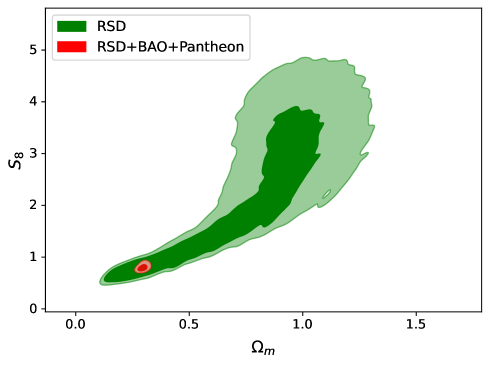
Figure 1: We show here the large degeneracy in parameter space the RSD data allow for the MTMG model and how instead BAO and Pantheon data effectively reduce it.

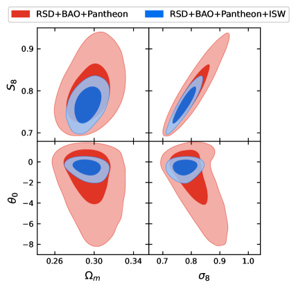
Figure 2: We show here that MTMG is sensitive also to ISW data, as the allowed parameter space further shrinks after we make use of them.

It should be noticed that at 68% CL, we have $\theta_{0}=-0.55_{-0.37}^{+0.61}$, which clearly states that: 1) $\Lambda$CDM is inside the 1-$\sigma$ level and 2) positive values for the mass of the graviton are well inside this allowed range of values. Now we can move on to study whether and how Planck will influence the final results.

VI.2 Data including Planck

We are now ready to analyze MTMG in the light of Planck data. Let us remind the reader that we have to sample a $\chi^{2}$ which is a function of eleven free parameters, namely

$$\chi^{2}=\chi^{2}(\omega_{b},\omega_{{\rm cdm}},\theta_{s},A_{s},n_{s},\tau_{{\rm reio}},A_{1},A_{2},\bar{c}_{1},\bar{c}_{2},\bar{c}_{3})\,,$$ (82)

where the first six ones are the same as in $\Lambda$CDM. The remaining five parameters are the new parameters introduced in MTMG in order to give a quite large class of possibilities in dynamics. Having eleven parameters, five more than $\Lambda$CDM, would give the idea that the constraints we obtains will not be so tight. This expectation is only partially true. Actually, the mass of the graviton, which is a function of the MTMG parameters and which is a derived parameter, directly and strongly affects the behavior of gravity and the structure formation (i.e. perturbations) so that, in fact, we obtain what we think is the strongest constraint on the mass of the graviton for the normal branch of MTMG.

In order to achieve this goal, and to see whether Planck data in the context of MTMG was suffering from tensions with the other data sets we have considered here, we have first of all made a run only using Planck data. The results for all the parameters of interest are shown in Table 2 and Fig. 3. In particular, in Fig. 3b, we can see that, thanks to Planck data, both positive and negative values for $\theta_{0}$ are still allowed but a large chunk of the negative parameter space is now not available any longer.

In the second and third steps we perform the $\chi^{2}$ adding BAO+Pantheon and then RSD+ISW as well. After marginalization over the parameters, for the constraint on $\theta_{0}$ at 68% CL we find $\theta_{0}=0.119_{-0.098}^{+0.12}$. This result shows that Planck tends to prefer non-negative values for the squared mass of the graviton, i.e. Planck prefers non-tachyonic gravitons in MTMG. Since, at 95% CL, we have $\theta_{0}=0.12_{-0.22}^{+0.21}$, then we can exclude all values for which $\theta_{0}<-0.1$ and $\theta_{0}>0.33$, which does not exclude $\Lambda$CDM. Furthermore, we find at 95% CL the following constraint on today’s squared mass for the graviton $\mu_{0}^{2}=2.5{}_{-4.8}^{+4.5}\times 10^{-67}\ {\rm eV}^{2}$, which implies, in particular, an upper bound $\mu_{0}<8.4\times 10^{-34}$ eV. We finally show for the joint analysis of all the data the 95% CL for $\mu_{0}^{2}$ in Fig. 4. We add the information on how MTMG is sensitive to the value of today’s Hubble parameter, and how both $S_{8}$ and $\theta_{0}$ are related to it in Fig. 5.

If the constraints on today’s value for the mass of the graviton turn out to be quite stringent (because most of the late time data sets are sensitive to it, i.e. they put constraints on the positive parameter$A_{1}$ on which $\mu_{0}$ also depends), we should expect that the value of the graviton mass at high redshifts should be less constrained as only Planck can sets some constraints on it. In fact at 95% CL we find $\mu_{{\rm\infty}}^{2}=0_{-69}^{+44}\times 10^{-67}{\rm eV}^{2}$.

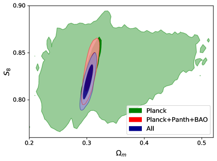
(a) Constraints/predictions on the variable $S_{8}$.

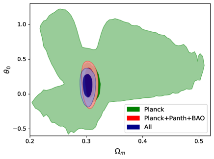
(b) Constraints on $\theta_{0}=\mu_{0}^{2}/H_{0}^{2}$, where $\mu_{0}^{2}$ is today’s squared mass of the graviton.

Figure 3: Analysis of Planck data, alone and together with BAO+Pantheon and further adding RSD+ISW.

	Planck	Planck+BAO+Pantheon	All joint analysis
$10^{2}\omega_{b}$	$2.242_{-0.030}^{+0.031}$	$2.242_{-0.027}^{+0.027}$	$2.247_{-0.027}^{+0.027}$
$\omega_{{\rm cdm}}$	$0.1197_{-0.0028}^{+0.0028}$	$0.1195_{-0.0020}^{+0.0020}$	$0.1189_{-0.0019}^{+0.0019}$
$100\theta_{s}$	$1.04194_{-0.00058}^{+0.00059}$	$1.04194_{-0.00056}^{+0.00056}$	$1.04198_{-0.00056}^{+0.00057}$
$\ln 10^{10}A_{s}$	$3.044_{-0.032}^{+0.032}$	$3.045_{-0.032}^{+0.033}$	$3.037_{-0.031}^{+0.031}$
$n_{s}$	$0.9671_{-0.0088}^{+0.0090}$	$0.9674_{-0.0076}^{+0.0077}$	$0.9683_{-0.0075}^{+0.0074}$
$\tau_{{\rm reio}}$	$0.055_{-0.015}^{+0.016}$	$0.055_{-0.015}^{+0.016}$	$0.052_{-0.015}^{+0.015}$
$A_{1}$	$0.57_{-0.57}^{+1.1}$	$0.63_{-0.63}^{+0.73}$	$0.71_{-0.71}^{+0.43}$
$A_{2}$	$6.2_{-7.0}^{+8.4}$	$6.4_{-6.4}^{+8.5}$	$3.9_{-3.9}^{+11}$
$\bar{c}_{1}$	$0.0_{-9.2}^{+9.2}$	$0.2_{-9.2}^{+9.0}$	$-0.1_{-8.5}^{+8.3}$
$\bar{c}_{2}$	$0.1_{-8.4}^{+8.4}$	$0.0_{-8.3}^{+8.5}$	$-0.4_{-7.1}^{+6.8}$
$\bar{c}_{3}$	$1.2_{-8.1}^{+8.1}$	$1.1_{-8.0}^{+8.2}$	$0.9_{-6.5}^{+6.6}$
$\Omega_{m}$	$0.318_{-0.068}^{+0.17}$	$0.306_{-0.012}^{+0.012}$	$0.302_{-0.011}^{+0.011}$
$H_{0}$	$67_{-10}^{+8}$	$68.11_{-0.92}^{+0.92}$	$68.37_{-0.93}^{+0.87}$
$\sigma_{8}$	$0.816_{-0.15}^{+0.089}$	$0.822_{-0.018}^{+0.021}$	$0.816_{-0.017}^{+0.016}$
$S_{8}$	$0.832_{-0.040}^{+0.040}$	$0.830_{-0.027}^{+0.028}$	$0.819_{-0.024}^{+0.023}$
$\Delta$	$-0.4_{-4.2}^{+2.7}$	$-0.4_{-4.1}^{+2.5}$	$-0.1_{-1.5}^{+1.3}$
$\theta_{0}$	$0.18_{-0.40}^{+0.64}$	$0.16_{-0.28}^{+0.27}$	$0.12_{-0.22}^{+0.21}$
$\bar{c}_{4}$	$3_{-10}^{+10}$	$3_{-11}^{+11}$	$3.2_{-6.9}^{+5.9}$

Table 2: Constraints at 95% CL on the primary and derived parameters of dynamical MTMG.

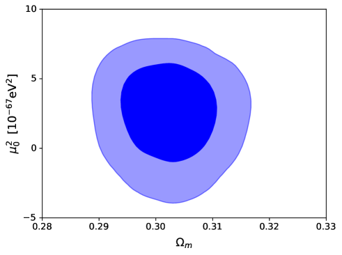
Figure 4: Constraints on $\mu_{0}^{2}$ for the joint analysis.

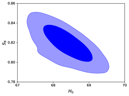
(a) Constraints on the variable $S_{8}$ as a function of $H_{0}$ in MTMG.

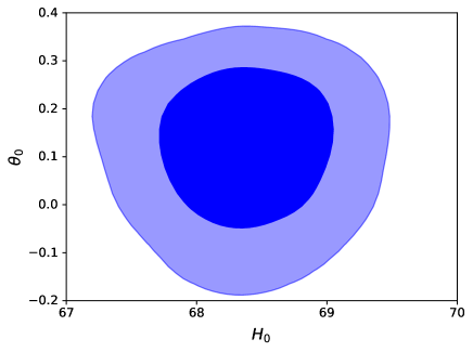
(b) Constraints on $\theta_{0}=\mu_{0}^{2}/H_{0}^{2}$ as a function of $H_{0}$ in MTMG.

Figure 5: Predictions given by the theory of MTMG regarding the observables $\theta_{0}$, $S_{8}$ and $H_{0}$.

VII Conclusions

The minimal theory of massive gravity (MTMG) is a theory with only two gravitational degrees of freedom which reproduces the dRGT massive gravity background for a homogeneous and isotropic universe without leading to ghost or strong coupling in general. As reminiscent of dRGT, the theory on a cosmological background allows for the presence of two branches, which are defined by the following background constraint (which comes in addition to the modified Einstein equations):

$$(c_{1}X^{2}+2c_{2}X+c_{3})\left(\frac{\dot{X}}{N}+HX-H\,\frac{M}{N}\right)=0\,,$$ (83)

where $N$ and $M$ are the physical and fiducial lapse respectively, $c_{i}$ ($i=1,2,3$) are free parameters of the theory, $H=\dot{a}/(aN)$ is the Hubble expansion rate, whereas $X=\tilde{a}/a$ is the ratio between the fiducial and the physical scale factors.

The self-accelerating solution, the one which fixes $X$ to be the constant satisfying $c_{1}X^{2}+2c_{2}X+c_{3}=0$, is indistinguishable from $\Lambda$CDM except for the tensor modes dynamics which acquire a non-zero mass. Therefore for this self-accelerating branch we can only assume the standard graviton-mass bounds to hold and they are trivially fulfilled once we impose from cosmological purposes that such a graviton mass is of order of $H_{0}$. In this latter case the self-accelerating branch of MTMG is trivially consistent with all experiments and observations, leaving no detectable imprint in the present data.

On the other hand, for the normal branch of MTMG, we need the equation $\frac{\dot{X}}{N}+HX-H\,\frac{M}{N}=0$ to hold. Since the fiducial metric (in the unitary gauge) corresponds to a given external field (that we fix to be homogeneous and isotropic, and only time-dependent, as to respect the symmetry of the FLRW background), it does not have its own dynamics and is a part of the definition of the theory. In particular on giving $X=X(z)$, Eq. (83) then uniquely fixes $M$ and from this point onward the theory will have its own phenomenological predictions which can be tested against the data.

We have thus studied the normal branch of MTMG in order to understand its predictions against some of the most recent and updated cosmological data. Although this in principle means to study the functional freedom of $X(t)$, in practice we have found it convenient to consider a simple model which describes a smooth three-parameters transition between two different values of $X$. In other words this model interpolates between two different values of the mass of the graviton, one describing the mass at high redshifts and the other one corresponding to today’s value for the mass of the graviton. Although this transition is still a special dynamics among all the possible ones, we think it captures the observationally relevant possibilities of the whole MTMG model for several reasons: (i) the background corresponds to a transition between two $\Lambda$CDM backgrounds (which differ by their effective cosmological constant), and we know that $\Lambda$CDM has still an extremely good fit to the data, and, although not impossible, it is quite hard to outperform it (see e.g. [24]); (ii) the final results on today’s value of the graviton mass $\mu_{0}$ closely agree with the ones recently shown in [20] for the simplest possible choice that $X(t)={\rm constant}$, namely the case where the background (but not the perturbations) is exactly the same as in $\Lambda$CDM. For these reasons we believe that the constraints we have found for the today’s graviton mass for the normal branch of MTMG will hold even for other dynamics of $X(t)$, after we impose all the constraints coming from the data.

After implementing the full Boltzmann equations for the perturbations, and on studying several data sets (and several combinations of them) which include Planck 2018, Pantheon (Supernovae Type Ia), baryonic acoustic oscillations (BAO), redshift space distortion (RSD), and ISW-galaxy correlation data sets, we have arrived at the following conclusions. First of all, inside these data sets MTMG does not feel any internal tension, so that all the data sets constrain the model in the most efficient way. Furthermore, although we use Planck 2018 and even if we have five new parameters (compared to $\Lambda$CDM), still we find strong constraint on today’s value of the graviton mass, to which most of the late-time data are sensitive. We then find that, at 95% CL, today’s squared mass for the graviton is bound to be in the following range: $\mu_{0}^{2}=2.5{}_{-4.8}^{+4.5}\times 10^{-67}\ {\rm eV}^{2}$, see also Fig. 4.

This result does not evidently rule out $\Lambda$CDM (for which $\mu_{0}$ vanishes), but rather, it gives a very interesting upper bound for the graviton mass in the normal branch of MTMG as $\mu_{0}<8.4\times 10^{-34}$ eV, which is the strongest so far for an existing theory of massive gravity. We hope this result will motivate further new studies in the field of massive gravity from both theoretical and phenomenological sides.