Passivity-based Local Criteria for Stability of Power Systems with Converter-Interfaced Generation

Abstract

With the increasing penetration of converter-interfaced distributed generation systems, it would be advantageous to specify local compliance criteria for these devices to ensure the small-signal stability of the interconnected system. Passivity of the device admittance, which is an example of a local criterion, has been used previously to avoid resonances between these devices and the lightly damped oscillatory modes of the network. Typical active and reactive power control strategies like droop control and virtual synchronous generator control inherently violate the passivity constraints on admittance at low frequencies, although this does not necessarily mean that the interconnected system will be unstable. Therefore, passivity of the admittance is unsuitable as a stability criterion for devices that are represented by their wide-band models. To overcome this problem, this paper proposes the use of criteria based on admittance at higher frequencies and an alternative transfer function at lower frequencies. The alternative representation uses active and reactive power and the derivatives of the polar components of voltage as interface variables. To allow for the separate analysis at low and high frequencies, the device dynamics should exhibit a slow-fast separation; this is proposed as an additional constraint. Adherence to the proposed criteria is not onerous and is easily verifiable through frequency response analysis.

I Introduction

A power system consists of a large number of devices like conventional and renewable energy generators, storage systems, loads, FACTS and HVDC converters, which are connected to the Transmission & Distribution (T&D) network. Sometimes, adverse dynamic interactions between these devices and the network occur, leading to oscillatory instabilities such as power swings, Sub-synchronous Resonance (SSR), Sub-synchronous Control Interactions (SSCI), Sub-synchronous Torsional Interactions (SSTI), Harmonic Resonances and Induction Generator effect [1, 2, 3, 4]. These instabilities may be anticipated and mitigated with the help of stability assessment tools like time-domain simulation and eigenvalue analysis.

Stability assessment generally needs to consider a large set of operating conditions of the network and the connected devices. A fresh analysis has to be done whenever the connection of a new device to the network is contemplated. Besides this, detailed information of the control structures and parameters are needed to carry out stability analysis. Some of these challenges can be alleviated by the use of a reduced system for the analysis. However, significant effort and engineering judgement are involved in determining the extent of the reduced study zone and the representation of the rest of the system by equivalents at its boundaries. The problem has become even more challenging with the proliferation of distributed generation systems, many of which have non-standardized controllers. Therefore, the possibility of specifying local (decentralized) criteria which, if complied with by individual devices, would ensure the stability of the interconnected system, has great appeal.

Although local criteria are likely to be conservative (sufficient, but not necessary for ensuring stability), this is acceptable as long as the criteria are not onerous or infeasible. The criteria should be such that compliance is easily verifiable through time-domain or frequency-domain analyses based on models or measurements. The main objective of this paper is to develop a set of criteria which has these attributes. Passivity [5] is a property of dynamical systems on which such criteria can be based. It is well-suited for this role because of the following reasons:

(a) Passive systems are stable.

(b) The system formed by the connection of passive sub-systems is also passive. Therefore the passivity of each sub-system can be individually ascertained with minimal information about the other sub-systems. If all connected sub-systems are passive, then unstable interactions among them are automatically precluded.

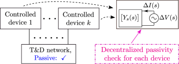
Figure 1: Passivity based stability assessment

(c) The model of a T&D network consisting of transmission lines, transformers, capacitors and inductors is inherently passive when it is formulated with currents and voltages as interface (input or output) variables. Topological changes in the network (for example, due to the addition/tripping of lines) or changes in the operating conditions do not affect the passivity of the network. The main objective then is to have each of the sub-systems that are connected to the T&D network locally conform to the passivity constraint, as depicted in Figure 1.

(d) The definition of a sub-system can be flexible; it could be an individual device or may encompass a sub-network with several devices. What matters is whether the sub-system is passive as seen from its boundary nodes.

(e) For linear time-invariant (LTI) systems, passivity can be conveniently ascertained using frequency domain conditions. Note that LTI models are appropriate for the study of many adverse interactions, as these can often be traced to small-signal instabilities.

The “self-disciplined stabilization” concept presented in [6] is similar to the scheme envisaged in Figure 1, but is applied to the Single-Input Single-Output devices in a dc microgrid. In three-phase ac systems, the models are Multi-Input Multi-Output, and the analysis is more involved. Passivity has been applied in a limited and approximate manner for the stability analysis of voltage source converter (VSC) based devices [7, 8, 9, 10, 11, 12] and HVDC converters [13]. In these papers, passivity is sought to be achieved locally around the network resonant frequencies only, and is not explored over the entire frequency domain. This requires knowledge of the parameters of the grid and other devices connected to it, because the combined system determines the resonant frequencies.

The passivity of converters and synchronous machines with their controllers are analysed in [14]. The synchronously rotating (D-Q) coordinate system is found to be convenient for developing the LTI models used in the analysis. Passivity of the admittance in D-Q variables appears to be a reasonable and achievable objective for the high-frequency models of the devices. It is also shown in the same paper that the admittances of typical active and reactive power injection devices inherently violate the passivity constraints at low frequencies, although this does not imply instability. Therefore, the passivity constraints on admittance are too restrictive for wide-band device models. To overcome the aforementioned difficulty, this paper proposes an expanded set of criteria which preserves the decentralized nature of the scheme. These criteria are given below:

1. The poles of the device transfer function should be separable into two well-separated clusters based on their magnitude. In other words, the natural transients should exhibit a slow-fast separation in the time domain (low and high frequency separation in the frequency domain).

2. The admittance transfer function should satisfy the frequency-domain passivity conditions in the high frequency range.

3. The transfer function between the derivatives of the polar coordinates of voltage and the active and reactive power drawn should satisfy the frequency-domain passivity conditions in the low frequency range.

Since most control strategies and transients in a power system exhibit time-scale separation characteristics, the first criterion is not unreasonable. Avoidance of grid resonances in the high frequency domain through passivity has already been demonstrated in earlier work. It is shown in this paper that in the low frequency range, with the specified set of interface variables, devices having typical droop-control or virtual synchronous machine characteristics can be made passive.

Compliance with the criteria can be verified numerically using frequency-domain techniques. Where analytical models or the internal details of the device and controller are not available, black-box simulation models or measurements may be used for obtaining the frequency responses. A case study of a converter-interfaced device is presented to illustrate the feasibility of this scheme.

II Passivity Definition

A system having a set of inputs $u(t)$ and an equal number of outputs $y(t)$ is said to be passive [5] if,

$$u(t)^{T}y(t)\geq\derivative{S(x)}{t}$$ (1)

for all $u(t)$ and $x(t)$, and for all $t\geq 0$, and where $S(x)$ is a continuously differentiable positive semi-definite function of the states $x$. $S(x)$ is also called the storage function.

II-A Passivity of LTI Systems (Time-Domain Conditions)

A LTI system represented by the state space model ($A$, $B$, $C$, $D$), is passive if there exist matrices $P$, $Q$ and $W$ such that [5]

$$PA+A^{T}P =-Q^{T}Q,$$ (2)

$$PB=C^{T}-Q^{T}W \;\;\text{and}\;\;D+D^{T}=W^{T}W$$

where the matrix $P$ is symmetric positive definite.

II-B Passivity of LTI Systems (Frequency-Domain Conditions)

A LTI system represented by a $n\times n$ rational, proper transfer function matrix $G(s)$ is passive if

1. there are no poles in the right half $s$-plane (complex plane).

2. The matrix $G^{\mathcal{R}}(j\Omega)=G(j\Omega)+G^{H}(j\Omega)=G(j\Omega)+G^{T}(-j\Omega)$ is positive semi-definite for all $\Omega\in(-\infty,\infty)$ which is not a pole of $G(s)$. $G^{\mathcal{R}}(j\Omega)$ is a Hermitian matrix, and therefore it will always have real eigenvalues. These should be non-negative for positive semi-definiteness [15].

3. For all $j\Omega_{p}$ that are poles of $G(s)$, the poles must be simple [16] and $\lim_{s\to j\Omega_{p}}(s-j\Omega_{p})\;G(s)$ should be positive semi-definite Hermitian.

For LTI systems, the frequency domain conditions are equivalent to those given in (1) and (2). Unlike (1) and (2) which require us to find a suitable storage function $S(x)$ or a set of matrices ($P$, $Q$ and $W$) - which is not straight forward - the frequency domain conditions are convenient from a practical perspective since they can be directly evaluated.

II-C Useful Properties

The usefulness of passivity criterion for stability assessment stems from the following properties.

1. Passivity is a sufficient condition for stability.

2. The inverse of a passive system is also passive, assuming that the state-space representation of the inverse system is well-defined.

3. A system formed by a negative feedback connection of passive sub-systems is also passive.

III Application to Power Systems

In this section, we outline the important steps and issues in the application of the passivity criterion (see  [14] for a detailed exposition). The first step in the application of passivity criteria is the formation of LTI models of the devices. Most power system devices are time-invariant or approximately so when expressed in the D-Q-o variables that are obtained using a synchronously rotating transformation [17] of the phase (a-b-c) variables. The models are linearized around a few operating points which are representative of the range of the device’s operation. The passivity check for the device has to be applied at each of these operating points.

The terminal currents and voltages are the “natural” interface (input and output) variables in an electrical system, as depicted in Figure 1. With these interface variables, a T&D network consisting of transmission lines, transformers, reactors and capacitors is inherently passive. The storage function for this system can be chosen to be the electro-magnetic energy stored in the inductive and capacitive components, which is dissipated in the resistive parts of these components. Topological changes in the network (due to the addition or removal of lines), or changes in the operating conditions do not affect the passivity of the network.

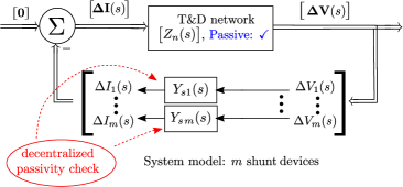
Figure 2: Transfer function representation of the system

The inherent passivity of the T&D network facilitates the decentralized scheme envisaged in Figure 1, as the task reduces to local assessment of the passivity of the devices/sub-systems connected to the network. The system shown in Figure 1 can be represented as a transfer function block diagram as shown in Figure 2.

For the $i^{th}$ single-port three-phase shunt device, $\Delta I_{i}=[\Delta i_{Di}\;\Delta i_{Qi}]^{T}$ and $\Delta V_{i}=[\Delta v_{Di}\;\Delta v_{Qi}]^{T}$ denote the D-Q components of the terminal currents and voltages respectively, and $\Delta I_{i}(s)$ = $Y_{si}(s)$ $\Delta V_{i}(s)$ defines the admittance matrix of the device. The transfer functions $Y_{si}(s)$ are matrices of size $2\times 2$ for single-port three-phase devices.

Once the admittance transfer function matrices are available, passivity can be assessed by checking their compliance to the conditions given in Section II-B. The frequency response of the transfer function matrices can be obtained either from an analytical model, or from experimental measurements, or applying the frequency scanning technique [13] to a simulation model of the system.

IV Limitation of D-Q Admittance Formulation

The scheme depicted in Figure 1 is based on the premise that it is possible to make all devices or sub-systems passive, if they are not so to begin with. The results in [7]–[14] indicate that the frequency domain conditions of Section II-B can usually be satisfied by the D-Q admittance of typical power system components in the high frequency range. However, it is also shown in [14] that the passivity conditions on the D-Q admittance are invariably violated in the low frequency range by many devices. For converter-interfaced devices, this is due to the commonly-used active and reactive power control strategies, as discussed in the following sub-sections.

IV-A Droop Control Strategy

The polar components of the bus voltage ($\phi,V_{n}$) and the active ($P$) and reactive power ($Q$) absorbed by the device are related to the D-Q voltage and current components as follows.

$$\phi =\tan^{-1}\left(\frac{v_{D}}{v_{Q}}\right),\,V=\sqrt{v_{D}^{2}+v_{Q}^{2}},\,V_{n}=\frac{V}{V_{o}}$$ (3)

$$P =v_{D}i_{D}+v_{Q}i_{Q},\,Q=v_{D}i_{Q}-v_{Q}i_{D}$$

The subscript ‘$o$’ denotes the quiescent value. The steady state active and reactive power drawn or injected by a wide class of power system components are often functions of frequency and voltage magnitude. The quasi-static model of a controlled device which follows a droop strategy is as follows.

$$\Delta P(s)=k_{pf}\,\Delta\tilde{\omega}(s)=k_{pf}\frac{s\;\Delta\phi(s)}{1+s\tau},\,\,\Delta Q(s)=k_{qv}\,\Delta V_{n}(s)$$ (4)

$\tau$, which is the time constant of the transfer function to approximately compute the derivative of the phase angle, is generally quite small.

Property 1.

The admittance corresponding to the small-signal model of a converter which emulates (4) is non-passive.

IV-B Virtual Synchronous Generator (VSG) Control Strategy

The VSG strategy is an alternative strategy for active and reactive power control of grid-connected converters. The controller is designed to emulate the characteristics of the classical model of a synchronous generator which is described by the following equations,

$$\frac{d\delta}{dt} =\omega_{r}-\omega_{o},$$ (5)

$$M\frac{d\omega_{r}}{dt} =P_{m}-D_{m}\omega_{r}+(v_{Q}i_{Q}+v_{D}i_{D})$$

$$v_{Q}+jv_{D} =E_{g}\angle\delta+jx_{g}(i_{Q}+ji_{D})$$

where $M,D_{m},\omega_{r},\delta,x_{g}$ denote the inertia, mechanical damping, electrical speed (in rad/s), rotor angle and transient reactance of the machine, and $E_{g}$ is constant.

Property 2.

The admittance corresponding to the small-signal model of a converter which emulates (5) is non-passive.

The proofs of these properties are given in [14]. These properties hold true regardless of the direction of power flow.

Illustrative Example: The non-passivity of the admittance in the low frequency region is illustrated in Figure 3. Two devices are considered: a VSC-based STATCOM that regulates terminal voltage using a PI controller and a VSC emulating a synchronous machine. The controller parameters of the STATCOM are as given in [18]. Note that passivity is inferred through the computation of the frequency-dependent eigenvalues of $Y_{s}^{\mathcal{R}}(j\Omega)=Y_{s}(j\Omega)+Y_{s}^{T}(-j\Omega)$, where $Y_{s}(j\Omega)$ denotes the admittance of the devices. One of the eigenvalues is negative in the lower frequency range (below 10 Hz), indicating that the conditions for passivity are not satisfied.

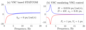
Figure 3: Eigenvalues of $Y_{s}^{\mathcal{R}}(j\Omega)$

Remarks: Passivity is a sufficient criterion for stability and not a necessary one. The conservative nature of passivity can be an acceptable trade-off against the benefits of having a convenient-to-use local criterion, provided passivity is achievable. The foregoing analysis shows that passivity of the admittance is impossible to achieve with typical control strategies of converter-interfaced devices, although it is well known that an interconnected system with these devices can be operated stably. Since these control strategies are essential for voltage and frequency regulation, they cannot be abandoned or radically changed. Hence there is a need to modify and/or expand the local criteria, and explore alternative transfer function formulations.

V Alternative Formulations based on Active and Reactive Power and Polar Coordinates of Voltage

Since the low frequency behaviour of devices is often associated with strategies to regulate voltage magnitude and frequency, an alternative formulation with the active and reactive power drawn by the device ($\Delta P$, $\Delta Q$), and the polar components of the bus voltage ($\Delta\phi$, $\Delta V_{n}$) as the interface variables, as defined in (3) is considered here. A related pair of interface variables is also considered, namely, the measured frequency and the derivative of $V_{n}$ as given below.

$$\Delta\tilde{\omega}(s)=\frac{s\,\Delta\phi(s)}{1+s\tau},\;\;\;\;\Delta\tilde{V}_{n}^{d}(s)=\frac{s\;\Delta V_{n}(s)}{1+s\tau}$$ (6)

The derivatives that are used in the computation of (6) are approximate; they preserve the proper-ness of the transfer functions.
The nomenclature for the various transfer function matrices employed in the following analyses are given in Table I.

Input variable	Output variable	Transfer function	Sub-system	Inverse system
Model I
$\begin{bmatrix}\Delta i_{D}(s)\\ \Delta i_{Q}(s)\end{bmatrix}$	$\begin{bmatrix}\Delta v_{D}(s)\\ \Delta v_{Q}(s)\end{bmatrix}$	$Z_{n}(s)$	Network	$Y_{n}(s)$
		$Z_{s}(s)$	Shunt device	$Y_{s}(s)$
Model II
$\begin{bmatrix}\Delta\phi(s)\\ \Delta V_{n}(s)\end{bmatrix}$	$\begin{bmatrix}\Delta P(s)\\ \Delta Q(s)\end{bmatrix}$	$J_{n}(s)$	Network	$\mathcal{N}_{n}(s)$
		$J_{s}(s)$	Shunt device	$\mathcal{N}_{s}(s)$
Model III
$\begin{bmatrix}\Delta\tilde{\omega}(s)\\ \Delta\tilde{V}_{n}^{d}(s)\end{bmatrix}$	$\begin{bmatrix}\Delta P(s)\\ \Delta Q(s)\end{bmatrix}$	$J_{nd}(s)$	Network	$\mathcal{N}_{nd}(s)$
		$J_{sd}(s)$	Shunt device	$\mathcal{N}_{sd}(s)$

Table I: Nomenclature for transfer function matrices

V-A Model II: ($\Delta P$,$\Delta Q$)-($\Delta\phi$,$\Delta V_{n}$) as input-output variables

It is essential to check whether the stability of the overall system with (a) D-Q currents and voltages and (b) ($\Delta P$, $\Delta Q$) and ($\Delta\phi$, $\Delta V_{n}$) as the input-output variables are equivalent. The following property clarifies this point.

Property 3.

Stability of the closed loop systems of Model I and Model II are equivalent, as the poles of the transfer functions are the same.

Proof.

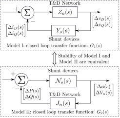
Figure 4: Stability of Model I and Model II

The expression of $G_{1}(s)$ is given as follows.

$$G_{1}(s)=\left(Y_{n}(s)+Y_{s}(s)\right)^{-1}\quad\text{where }Y_{n}(s)=(Z_{n}(s))^{-1}$$

The transfer functions of the individual components of Model I and Model II are related as follows.

$$\begin{aligned} J_{n}(s)=\left(\mathcal{E}Y_{n}(s)+\mathcal{C}\right)\mathcal{F},\,J_{s}(s)=\left(\mathcal{E}Y_{s}(s)-\mathcal{C}\right)\mathcal{F}\end{aligned}$$ (7)

where

$$\begin{aligned} \mathcal{E}=\begin{bmatrix}v_{Do}&v_{Qo}\\ -v_{Qo}&v_{Do}\end{bmatrix}&,\,\mathcal{C}=\begin{bmatrix}i_{Do}&i_{Qo}\\ i_{Qo}&-i_{Do}\end{bmatrix},\mathcal{F}=\begin{bmatrix}v_{Qo}&v_{Do}\\ -v_{Do}&v_{Qo}\end{bmatrix}\end{aligned}$$ (8)

The closed loop transfer function of Model II is as follows.

$$G_{2}(s) =\left(J_{s}(s)+J_{n}(s)\right)^{-1}=\mathcal{F}^{-1}\,G_{1}(s)\,\mathcal{E}^{-1}$$ (9)

The expressions here are derived using (7). Since $\mathcal{F}$ and $\mathcal{E}$ are both invertible (except for $v_{Do}=v_{Qo}=0$), the poles of both $G_{1}(s)$ and $G_{2}(s)$ are identical. This implies that the stability of the two models are equivalent. ∎

The choice of different input and output pairs may result in passivity properties being different. For instance, the droop control strategy is passive when these interface variables are used because the transfer function matrix in the relationship

$$\mathcal{N}_{s}(s)=\begin{bmatrix}\frac{1+s\tau}{s}\times\frac{1}{k_{pf}}&0\\ 0&\frac{1}{k_{qv}}\\ \end{bmatrix}$$

satisfies the frequency domain passivity conditions. The T&D network may be represented as follows:

$$J_{n}(s)=\begin{bmatrix}J_{11}(s)&J_{12}(s)\\ J_{21}(s)&J_{22}(s)\end{bmatrix}$$

At low frequencies, the network transfer function can be approximated by $J_{LF}=J_{n}(s=0)$, which is the unreduced form of the load-flow Jacobian matrix. Normally $J_{LF}^{R}=J_{LF}+J_{LF}^{T}$ is singular (with one zero eigenvalue), because there cannot be a unique solution for the phase angles for specified set of active and reactive power injections. $J_{LF}^{R}$ may not be positive semi-definite either because the shunt capacitances in the network often result in a negative eigenvalue. This also implies that the network transfer function $J_{n}(s)$ may not be passive.

The non-passivity of $J_{LF}$ can be alleviated by requiring that some devices connected to the network “contribute” to the diagonal terms of $J_{22}$. This is in order to compensate the effect of the shunt capacitances. The compensation must be done by the devices without jeopardizing their own passivity. This idea is depicted in Figure 5. In practical terms, this means that at least some devices should contribute to voltage regulation through Q-V control, which is not a surprising requirement. The compensation, denoted by $k_{qv}^{c}$, has to be specified for each device by the T&D operator based on an evaluation of the eigenvalues of $J_{LF}^{R}$ and the ratings of the connected devices. The aim is to ensure that no eigenvalue of $J_{LF}^{R}$ is negative.

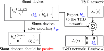
Figure 5: Contribution of devices to network passivity

Illustrative Example: The schematic of a network with controllable generators and loads is shown in Figure 6. The transmission line parameters and the equilibrium power flows are taken from the three-machine system of [19].

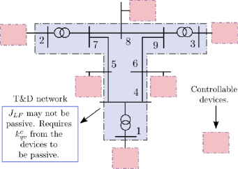
Figure 6: A network with controllable devices

The eigenvalues of $J_{LF}^{R}$ are given in Table II. $J_{LF}$ is not passive as $J_{LF}^{R}$ has a negative eigenvalue. If all the controllable generators and loads are able to contribute $k_{qv}^{c}=0.7$ pu, then $J_{LF}$ becomes passive, as shown in the table. Although the passivation of $J_{LF}$ is demonstrated here with equal contribution of $k_{qv}^{c}$ by all devices, it need not always be so in practice.

Base Case	Modified Case
$\mathbf{-0.84},0,7.52,8.50,10.15,$ $12.93,31.71,34.74,34.95,$ $36.29,41.37,42.8,93.51,94.52,$ $107.94,108.29,115.46,115.76$	$0,\mathbf{0.025},7.87,8.82,10.42,$ $13.13,32.43,35.06,35.44,36.53,$ $42.1,42.88,93.92,95.08,$ $108.29,109.06,115.72,116.61$
$k_{qv}^{c}$ contributions: 0.65 pu at buses 1, 2, 3, 5, 6, 8 each.

Table II: Eigenvalues of $J_{LF}^{R}$ of the three machine system

With this modification, passivity seems to be an achievable criterion for the network and the devices obeying the droop control strategy. However, Model II encounters problems with devices which emulate synchronous machines.

Property 4.

The transfer function matrix $\mathcal{N}_{s}(s)$ of a converter which emulates (5) is not passive. [See Appendix A.1 for the proof]

The network transfer functions considered in the analysis in this sub-section were based on a low frequency approximation, wherein the network was represented by a static model $J_{LF}$. However, the wide-band model of the network, $J_{n}(s)$, cannot be passivated because of the following property.

Property 5.

A R-L-C network will not satisfy the frequency domain passivity conditions at higher frequencies, with ($\Delta P$, $\Delta Q$) and ($\Delta\phi$, $\Delta V_{n}$) as input-output variables. [See Appendix B.1 for the proof]

V-B Model III: ($\Delta P$,$\Delta Q$)-($\Delta\tilde{\omega}$,$\Delta\tilde{V}_{n}^{d}$) as input-output variables

The following property brings out the equivalence of closed loop systems of Model I, Model II and Model III from a stability perspective.

Property 6.

The stability of closed loop systems represented by Models I, II and III are equivalent, provided that the closed loop system of Model I does not have repeated poles at $s=0$.

Proof.

Model III in Figure 7 represents the overall system model when the interface variables are chosen to be $(\Delta P,\Delta Q)$ and $(\Delta\tilde{\omega},\Delta\tilde{V}_{n}^{d})$. The closed loop transfer function of Model III is

$$G_{3}(s)=\frac{s}{(1+s\tau)}G_{2}(s).$$ (10)

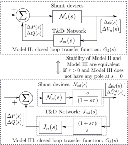
Figure 7: Stability of Model II and Model III

a) If there are no pole-zero cancellations on the RHS, then poles of $G_{3}(s)$ are the same as of $G_{2}(s)$, except for the additional stable pole at $s=-\frac{1}{\tau}$. In this case, both models are equivalent from a stability perspective.

b) A pole zero cancellation at $s=-\frac{1}{\tau}$ is not of concern since it is in the left half $s$-plane.

c) If $G_{2}(s)$ has a pole at $s=0$, which is cancelled by the zero at $s=0$ in (10), then the stability is not affected provided that the cancelled pole is simple (non-repeated). Note that if there is a non-simple pole of $G_{2}(s)$ at $s=0$, then $G_{2}(s)$ is unstable while $G_{3}(s)$ can be stable. ∎

Observation: The closed loop system with ($\Delta P$, $\Delta Q$) and ($\Delta\phi,\Delta V_{n}$) as the input-output pairs has non-simple (repeated) poles at $s=0$ only if all the converters emulating (5) have zero damping ($D_{m}$), and all converters emulating (4) have zero $k_{pf}$. As positive $D_{m}$ or $k_{pf}$ is introduced, one of the repeated poles at $s=0$ moves towards the left, and the pole at $s=0$ becomes simple. This can be understood in practical terms as follows: If $D_{m}$ and $k_{pf}$ are zero for all connected devices then the frequency will change monotonically if there is a load-generation imbalance. This situation can be avoided by having at least some devices with frequency regulation characteristics.

The advantage of using ($\Delta\tilde{\omega}$, $\Delta\tilde{V}_{n}^{d}$) is that passivity is a feasible objective for both droop-controlled devices and VSG-controlled devices, as is evident from the following property.

Property 7.

The transfer function matrix $\mathcal{N}_{sd}(s)$ of a converter which emulates (4) or (5) is passive, provided $\tau$ is small. [See Appendix A.2 and A.3 for proof]

As regards the network, the low frequency transfer function of the network can be related to $J_{LF}$ as

$$J_{nd}(s)=J_{LF}\times\frac{1+s\tau}{s}.$$

Note that $J_{nd}(s)$ has a simple pole on the $j\Omega$ axis (at $s=0$), thereby requiring compliance with condition (3) of Section II-B. If $J_{LF}$ is positive semi-definite hermitian after augmentation with the $k_{qv}^{c}$ contributed by the shunt devices (as discussed in Section V), then $J_{nd}(s)$ will satisfy the conditions of passivity at low frequencies. However, $J_{LF}$ is hermitian only for a lossless network. Since losses are generally small in a T&D network, they may be neglected in the analysis. In such a situation, the positive semi-definiteness of $J_{LF}$ implies that $J_{nd}(s)$ satisfies the passivity conditions at low frequency.

The wide band model of the network, $J_{nd}(s)$, is not passive because of the following property.

Property 8.

A R-L-C network will not satisfy the frequency domain passivity conditions at higher frequencies, with ($\Delta P$, $\Delta Q$) and ($\Delta\tilde{\omega}$, $\Delta\tilde{V}_{n}^{d}$) as input-output variables. [See Appendix B.2 for the proof]

VI Summary and Discussions

(a) The electrical T&D network consisting of transmission lines, transformers, inductors and capacitors is passive when Model I is used. Prior work indicates that the devices connected to the passive network can be made to satisfy the passivity conditions in the higher frequency range through controller modifications or by inclusion of some part of the passive external network. It is, however, impossible for most active and reactive power injection devices to comply with the passivity conditions in the lower frequency range, although the system may be stable after their connection in the network.

(b) With Model II, the passivity conditions are achievable in the low frequency range by models of devices that follow the droop control strategy. Although the low frequency network model may not be passive, it can be passivated by including within it some devices with voltage regulating ability (Q-V droop). However, it may be impossible for a high frequency network model to achieve the passivity conditions with these interface variables, although the overall system may be stable. Devices with synchronous machine-like characteristics are also not passive in these interface variables.

(c) With Model III, the devices with droop control characteristics or synchronous machine characteristics can be made to satisfy the passivity conditions in the low frequency range. As in the previous case, voltage control can passivate the low frequency model of the network, but the high frequency model would still be non-passive. Frequency regulation avoids the presence of repeated poles at $s=0$ in Model I, which is required for inferring its stability from that of Model III.

(d) Thus, Model I and Model III have mutually exclusive frequency ranges in which the compliance with the passivity conditions is achievable. However, passivity cannot be achieved by a single wide-band model representation, regardless of the stability of the system. A decoupled analysis for the low and high frequency approximations of the system could salvage this situation: the passivity based conditions could be applied to Model I at higher frequencies, while they could be applied to Model III at lower frequencies.

(e) Decoupled stability analysis of low and high frequency (slow and fast) approximations of the wide-band models is mathematically justifiable if they are non-interacting. A necessary condition for this is that the eigenvalues of the system should be separable into slow and fast clusters in the complex plane. The stability of the system with time-scale separated dynamics can be predicted from the independent analysis of the eigenvalue clusters [20].

(f) Slow-fast separation of dynamic behaviour is not an unreasonable requirement. In fact, most power system components have this inherent feature. Generally, network resonant frequencies are well removed from the modal frequencies associated with electro-mechanical dynamics [1, 17]. Controllers of power electronic converters generally have a hierarchical structure which has faster “inner loops” associated with current control and firing angle generation, and relatively slower “outer loops” for voltage regulation and power modulation. It is commonly observed in power system studies that the slow-fast eigenvalue separation of the individual devices and the network is preserved after they are interconnected. Hence the separability of eigenvalues of individual components is proposed here as an additional requirement to facilitate decoupled analysis.

Based on the foregoing discussions, the local stability criteria are consolidated and presented below.

1. Obtain the frequency response of the D-Q admittance matrix $Y_{s}(s)$ of the device. This may either be derived analytically or extracted numerically using the frequency scanning technique [18]. The scanning may be done over a wide frequency range that is larger than the controller bandwidth.

2. Obtain a state space model corresponding to $Y_{s}(s)$. A vector fitting algorithm [21] may be used for this purpose if the frequency response $Y_{s}(s)$ has been extracted numerically.

3. Ensure that the eigenvalues of the wide band model are well-separated, say with no eigenvalues having absolute values between 62.8 rad/s (10 Hz) and 220 rad/s (35 Hz).

4. Ensure that the admittance model (Model I) satisfies condition (2) of Section II-B in the higher frequency range ($\geq 35$ Hz).

5. Obtain $J_{s}(s)$ from $Y_{s}(s)$ using (7). Ensure that the real part of the (2,2) entry of $J_{s}(j\Omega)$ is $\geq k_{qv}^{c}$ in the lower frequency range ($\leq$ 10 Hz). $k_{qv}^{c}$ is a value specified by the network operator, as discussed in Section V-A.

6. After extracting $k_{qv}^{c}$, evaluate the transfer function matrix $J_{sd}(s)$, and subsequently evaluate $\mathcal{N}_{sd}(s)$. Ensure that the real part of the (1,1) term of $J_{sd}(s)$ is positive in the lower frequency range ($\leq$ 10 Hz) to avoid the presence of repeated poles at $s=0$ in the overall system, as discussed in Section V-B.

7. To ensure properness of $\mathcal{N}_{sd}(s)$, $(\mathcal{E}D+\mathcal{C})\mathcal{F}$ should be non-singular, where $D$ is the feedforward matrix of the state-space model obtained in (1), and $\mathcal{E},\mathcal{C}$ and $\mathcal{F}$ are as defined in (8).

8. Ensure that $\mathcal{N}_{sd}(s)$ satisfies condition (2) of Section II-B in the lower frequency range ($\leq 10$ Hz).

The application of the consolidated decentralized stability criteria is depicted in Figure 8. Note that compliance with the specified criteria is attempted through controller modifications. This may require several iterations until all the conditions are achieved for all the credible operating conditions.

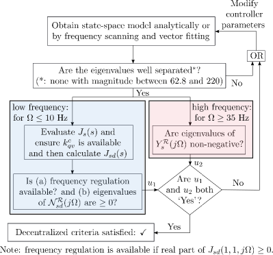
Figure 8: Application of the criteria for stability

(g) The criteria given here are not intended to be device-specific. However, it may not be possible to modify the controllers of some devices due to legacy issues. The dynamic characteristics of some devices may also be inherently passivity-resistant in the Model I and/or Model III formulations. For example, the transfer function $\mathcal{N}_{sd}(s)$ of certain loads are not passive (see Appendix A.4 for proof). In such scenarios, one may attempt to apply the criteria at the boundaries of a sub-system consisting of several devices and a part of the network. This may be done with the expectation that some passive devices will be able to compensate for the non-passivity of the others. If this cannot be achieved, then a conventional stability study of the interconnected system will become necessary. With the increased penetration of converter-interfaced devices with flexible controllers that can satisfy the local criteria, the need for such centralized small-signal stability studies can however be deferred or minimized.

VII Case Study: VSC based power injection

Consider a 200 MVA VSC based device connected to a T&D network via a transformer having leakage reactance equal to 0.15 pu. The dc side of the device is connected to a battery. The device is capable of exchanging both active and reactive power with the grid. The schematic of the controller is shown in Figure 9. The controller parameters are expressed in per unit. The current injected by the device is controlled by the well-known “vector control” scheme in the local (d-q) frame of reference [22].

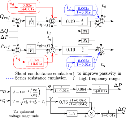
Figure 9: Schematic of VSC based device controller

The controller has the following supplementary blocks, which are intended to improve the passivity behaviour of the device:
(a) Blocks to mimic active series and shunt resistances which are included to improve the passivity of $Y_{s}(s)$ in the higher frequency range [23]. These are highlighted in blue and red.
(b) Voltage and frequency regulation are provided in the low frequency range, so that $\mathcal{N}_{sd}(s)$ is passive.

The device is operated at two different operating conditions. Case 1 represents an active power injection mode where the device injects active and reactive power of 0.7 pu and 0.25 pu respectively. Case 2 represents a reactive power compensation scheme (STATCOM application) where the device injects only 0.7 pu reactive power.

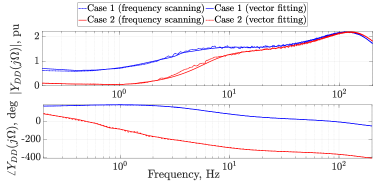
Figure 10: Frequency scanning and vector fitting model

The frequency response $Y_{s}(s)$ of the VSC based device is obtained in the range $(0.2-200)$ Hz using the frequency scanning technique [18]. The frequency response is fitted to a rational state-space model using the vector fitting algorithm [21]. The fitting is found to be accurate. To illustrate this, the frequency response of the (1,1) term of $Y_{s}(s)$, denoted by $Y_{DD}(s)$, and the same evaluated from the fitted model are shown in Figure 10.

Case	Clusters	Eigenvalues of fitted state space model
$P_{o}=0.7$ pu, $Q_{o}=0.25$ pu	Slow	$-0.99,-14.76,-3.61\pm j23.41,$ $-48.28\pm j27.99$
	Fast	$-450.27\pm j60.69,-575.78\pm j756.66$
$P_{o}=0$, $Q_{o}=0.7$ pu	Slow	$-0.89,-0.81\pm j5.58,-0.23\pm j9.57,$ $-14.36,-35.37\pm j31.06$
	Fast	$-317.44,-541.11,-593.69\pm j753.59$

Table III: Eigenvalues of the rational state-space model

The eigenvalues of the fitted rational state-space models are given in Table III. The poles are well-separated, which facilitates the separate analysis of the faster and slower transients. The passivity of the admittance is evaluated and is shown in Figure 11. Note that $Y_{s}(s)$ satisfies the passivity conditions in the higher frequency range ($\geq$ 32 Hz).

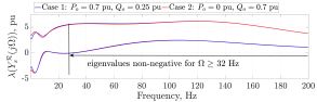
Figure 11: Eigenvalues of $Y_{s}^{\mathcal{R}}(j\Omega)$

The minimum amount of $k_{qv}$ (real part of the $(2,2)$ term of $J_{s}(s)$) available to be exported to the T&D network is shown in Figure 12. Note that it is capable of exporting at most $k_{qv}=2$ pu to the network in the low frequency range.

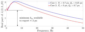
Figure 12: Minimum $k_{qv}$ available to export to the network

Assume that the network operator has specified that $k_{qv}^{c}$ = 0.4 pu needs to be exported to the network. After extraction of $k_{qv}^{c}=0.4$ pu from the frequency response, the frequency response matrix $J_{sd}(s)$ is calculated, with $\tau=0.01$. In order to check the frequency regulation capability in the lower frequency range, the real part of $J_{sd}(1,1,s)$ is plotted in Figure 13. Note that it is positive in the lower frequency range, which indicates that it can provide frequency regulation.

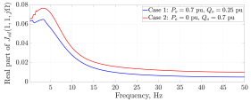
Figure 13: Frequency regulation in the low frequency range

The passivity of $\mathcal{N}_{sd}(s)$ in the lower frequency range is now verified in Figure 14. It can be seen that the eigenvalues of $\mathcal{N}_{sd}^{\mathcal{R}}(j\Omega)$ are non-negative in the low frequency range, indicating passivity compliance of $\mathcal{N}_{sd}(s)$.

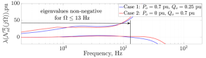
Figure 14: Eigenvalues of $\mathcal{N}_{sd}^{\mathcal{R}}(j\Omega)$

Figure 15: Schematic of the T&D network

The closed loop performance of the device is also verified by connecting it to a T&D network, whose schematic is shown in Figure 15. A 5% pulse change of duration 1 s is applied to the active power reference at $t=0.5$ s, and to the reactive power reference at $t=2$ s. The responses of the VSC based device are shown in Figure 17 and 17. It can be seen that the response is satisfactory with the tuned controller parameters.

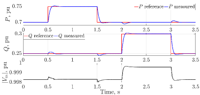
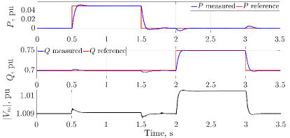
Figure 16: Case 1: 5% pulse change in $P_{ref}$ and $Q_{ref}$

Figure 17: Case 2: 5% pulse change in $P_{ref}$ and $Q_{ref}$

VIII Conclusions

This paper has developed decentralized compliance criteria for devices/sub-systems that ensure stability of the interconnected power system. These can be evaluated locally and individually for each converter based device with minimal information about the rest of the system. The proposed criteria are based on passivity. However, passivity alone is unsuitable for wide-band models as they would find it impossible to meet the passivity criterion. Hence additional criteria have to be specified to make the scheme feasible.

The criteria can be summarized as follows: (a) The devices should exhibit well-separated fast-slow dynamics. (b) The model of the devices should be passive in the higher frequency range, when formulated with the D-Q currents and voltages as the interface variables. (c) In the low frequency range, the devices should be passive when formulated with the active and reactive power, and the derivatives of the polar coordinates of voltage as the interface variables. Complying with the criteria is not onerous and is easy to verify in the frequency domain.

The increased penetration of converter-interfaced devices that comply with these local criteria could potentially reduce the need for frequently conducting centralized connectivity studies to ensure small-signal stability.

Appendix A Passivity of some Models

A-A Converters emulating (5): Passivity of $\mathcal{N}_{s}(s)$

The (1,1) element of $\mathcal{N}_{s}(s)$ is as follows.

$$\mathcal{N}_{s}(1,1,s)=\frac{1}{(Ms^{2}+D_{m}s)}+\frac{x_{g}(2V_{o}-E_{g}\cos\zeta_{o})}{E_{g}V_{o}(2V_{o}\cos\zeta_{o}-E_{g})}$$

where $\zeta_{o}=\delta_{o}-\tan^{-1}\left(\dfrac{v_{Do}}{v_{Qo}}\right)$.
Case I: $D_{m}\neq 0$: For typical values of $M,D_{m},x_{g},E_{g},V_{o},\delta_{o}$ and for smaller values of $\Omega$, the (1,1) entry of $\mathcal{N}_{s}^{\mathcal{R}}(j\Omega)=\mathcal{N}_{s}(j\Omega)+\mathcal{N}_{s}^{T}(-j\Omega)$ is as follows.

$$\mathcal{N}_{s}^{\mathcal{R}}(1,1,j\Omega)\approx-\frac{2M}{D_{m}^{2}}\quad\text{for $\Omega\to 0$}$$

Since this diagonal entry is negative, $\mathcal{N}_{s}(s)$ does not satisfy condition (2) of Section II-B at low frequencies. Therefore $\mathcal{N}_{s}(s)$ is not passive.
Case II: $D_{m}=0$: In this case, $\mathcal{N}_{s}(1,1,s)$ is as follows.

$$\mathcal{N}_{s}(1,1,s)=\frac{1}{Ms^{2}}+\frac{x_{g}(2V_{o}-E_{g}\cos\zeta_{o})}{E_{g}V_{o}(2V_{o}\cos\zeta_{o}-E_{g})}$$

This indicates the presence of non-simple (repeated) poles at $s=0$ (on the $j\Omega$ axis), which violates condition (3) in Section II-B. Therefore $\mathcal{N}_{s}(s)$ is not passive.

A-B Converters emulating (5): Passivity of $\mathcal{N}_{sd}(s)$

It can be shown that $\mathcal{N}_{sd}(s)=J_{d}(s)-\dfrac{s\tau}{1+s\tau}J_{d}(s)$ where

$$\begin{aligned} J_{d}(1,1,s)&=\frac{1}{(Ms+D_{m})}+\frac{sx_{g}(2V_{o}-E_{g}\cos\zeta_{o})}{E_{g}V_{o}(2V_{o}\cos\zeta_{o}-E_{g})}\\ J_{d}(1,2,s)&=J_{d}(2,1,s)=\frac{s\,x_{g}\,\sin\zeta_{o}}{V_{o}\,(2V_{o}\,\cos\zeta_{o}-E_{g})}\\ J_{d}(2,2,s)&=\frac{s\,x_{g}\,\cos\zeta_{o}}{V_{o}\,(2V_{o}\,\cos\zeta_{o}-E_{g})}\end{aligned}$$ (11)

where $\zeta_{o}=\delta_{o}-\tan^{-1}\left(\dfrac{v_{Do}}{v_{Qo}}\right)$. The poles of $\mathcal{N}_{sd}(s)$ are $-\frac{D_{m}}{M}$ and $-\frac{1}{\tau}$, and therefore it is stable. $J_{d}^{\mathcal{R}}(j\Omega)=J_{d}(j\Omega)+J_{d}^{T}(-j\Omega)$ is positive semi-definite because (a) the trace is $\frac{2D}{M^{2}\Omega^{2}+D^{2}}>0$, and (b) the determinant is zero for all $\Omega$.

Note that $\mathcal{N}_{sd}(s)\approx J_{d}(s)$ in the low frequency range, if $\tau$ is small. Since $J_{d}(s)$ is passive, it follows that $\mathcal{N}_{sd}^{\mathcal{R}}(j\Omega)$ will also be positive semi-definite, if $\tau$ is small. Hence $\mathcal{N}_{sd}(s)$ of converters that emulate (5) is passive if $\tau$ is small.

A-C Converters emulating (4): Passivity of $\mathcal{N}_{sd}(s)$

In this case, $\mathcal{N}_{sd}(s)$ is as given below.

$$\mathcal{N}_{sd}(s)=\begin{bmatrix}\frac{1}{k_{pf}}&0\\ 0&\frac{1}{k_{qv}}\times\frac{s}{(1+s\tau)}\end{bmatrix}$$

Note that $\mathcal{N}_{sd}^{\mathcal{R}}(j\Omega)\geq 0$ for all $\Omega$ if $k_{pf},k_{qv}>0$. This indicates that $\mathcal{N}_{sd}(s)$ of a converter that emulates (4) satisfies the passivity conditions.

A-D Voltage and Frequency Dependent Loads

For a load with load characteristics as given in (12),

$$\Delta P=k_{pf}\Delta\tilde{\omega}+k_{pv}\Delta V_{n},\,\,\Delta Q=k_{qf}\Delta\tilde{\omega}+k_{qv}\Delta V_{n}$$ (12)

the transfer function $\mathcal{N}_{sd}(s)$ is as given below.

$$\mathcal{N}_{sd}(s)=\frac{1}{(k_{pf}k_{qv}-k_{pv}k_{qf})}\begin{bmatrix}k_{qv}&-k_{pv}\\ -\frac{sk_{qf}}{(1+s\tau)}&\frac{sk_{pf}}{(1+s\tau)}\end{bmatrix}$$ (13)

$\mathcal{N}_{sd}(s)$ is not passive in general. For example, with $k_{pv}=0.07,k_{qv}=0.5,k_{pf}=0.006,$ and $k_{qf}=0.003$, which are the parameters of a typical industrial motor [1], $\mathcal{N}_{sd}^{\mathcal{R}}(j\Omega)$ is not positive semi-definite at $\Omega=0$.

Appendix B Passivity of $R$-$L$-$C$ network

Consider the D-Q admittance transfer function be denoted by $Y_{n}(s)$. If the state space matrices of the D-Q domain admittance are $(A_{n},B_{n},C_{n},D_{n})$, then

$$D_{n}=\lim_{s\to\infty}Y_{n}(s)=\begin{bmatrix}D_{1}&\mathbf{0}\\ \mathbf{0}&D_{1}\end{bmatrix}$$ (14)

Note that $D_{1}$ is symmetric.

B-A Interface variables: $(\Delta P,\Delta Q)$ – $(\Delta\phi,\Delta V_{n})$

If the state-space matrices of the transfer function matrix $J_{n}(s)$ are $(A_{j},B_{j},C_{j},D_{j})$, then $D_{j}$ is as follows.

$$D_{j}=\left(\mathcal{E}D_{n}+\mathcal{C}\right)\mathcal{F}$$ (15)

where $\mathcal{E},\mathcal{C}$ and $\mathcal{F}$ are defined as given in (8). Note that

$$D_{j}+D_{j}^{T}=2\begin{bmatrix}(i_{Do}v_{Qo}-i_{Qo}v_{Do})&(i_{Do}v_{Do}+i_{Qo}v_{Qo})\\ (i_{Do}v_{Do}+i_{Qo}v_{Qo})&-(i_{Do}v_{Qo}-i_{Qo}v_{Do})\end{bmatrix}$$

and therefore its trace is zero, indicating that it is not positive semi-definite. This violates the time domain conditions (see Section II-A). Therefore the system is not passive.

B-B Interface variables: $(\Delta P,\Delta Q)$ – $(\Delta\tilde{\omega},\Delta\tilde{V}_{n}^{d})$

If the state-space matrices of the transfer function matrix $J_{nd}(s)$ are $(A_{jd},B_{jd},C_{jd},D_{jd})$, then $D_{jd}=\tau(D_{j})$, where $D_{j}$ is as given in (15). Note that the trace of $D_{jd}+D_{jd}^{T}$ is zero, which violates the time domain conditions (see Section II-A). Therefore the system is not passive.

Kaustav Dey (STM’19) received his B.E. degree in Electrical Engineering from Jadavpur University, India in 2015. He is currently a Ph.D student in the Department of Electrical Engineering at the Indian Institute of Technology, Bombay. His research interests include power system dynamics, applications of signal processing and control systems in power systems.

A. M. Kulkarni (M’07, SM’19) received his B.E. degree in electrical engineering from the University of Roorkee in 1992. He obtained his M.E. degree in electrical engineering in 1994 and his PhD in 1998 from the Indian Institute of Science, Bangalore. He is currently a Professor at the Indian Institute of Technology, Bombay. His research interests include Power system dynamics, HVDC, FACTS and Wide Area Measurement Systems.

References

- [1] P. Kundur, Power system stability and control, 1st ed. McGraw Hill Education (India), New Delhi, 1994.
- [2] G. D. Irwin, A. K. Jindal, and A. L. Isaacs, “Sub-synchronous control interactions between type 3 wind turbines and series compensated AC transmission systems,” in IEEE Power Energy Soc. Gen. Meet., 2011, pp. 1–6.
- [3] K. R. Padiyar, Analysis of subsynchronous resonance in power systems, 3rd ed. Springer Science & Business Media, 2012.
- [4] J. D. Ainsworth, “Harmonic instability between controlled static convertors and ac networks,” in Proceedings of the Institution of Electrical Engineers, vol. 114. IET, 1967, pp. 949–957.
- [5] H. K. Khalil, Nonlinear Systems, 3rd ed. Prentice Hall, Upper Saddle River, New Jersey, 2002.
- [6] Y. Gu, W. Li, and X. He, “Passivity-Based Control of DC Microgrid for Self-Disciplined Stabilization,” IEEE Trans. Power Syst., vol. 30, no. 5, pp. 2623–2632, 2015.
- [7] X. Wang, F. Blaabjerg, M. Liserre, Z. Chen, J. He, and Y. Li, “An active damper for stabilizing power electronics-based AC systems,” in IEEE Appl. Power Electron. Conf. Expo., 2013, pp. 1131–1138.
- [8] X. Wang, Y. Pang, P. C. Loh, and F. Blaabjerg, “A Series-LC-Filtered Active Damper With Grid Disturbance Rejection for AC Power-Electronics-Based Power Systems,” IEEE Trans. Power Electron., vol. 30, no. 8, pp. 4037–4041, 2015.
- [9] L. Harnefors, L. Zhang, and M. Bongiorno, “Frequency-domain passivity-based current controller design,” IET Power Electronics, vol. 1, no. 4, pp. 455–465, 2008.
- [10] H. Bai, X. Wang, P. C. Loh, and F. Blaabjerg, “Passivity enhancement of grid-tied converters by series LC-filtered active damper,” IEEE Trans. Ind. Electron., vol. 64, no. 1, pp. 369–379, 2017.
- [11] L. Harnefors, M. Bongiorno, and S. Lundberg, “Input-admittance calculation and shaping for controlled voltage-source converters,” IEEE Trans. Ind. Electron., vol. 54, no. 6, pp. 3323–3334, 2007.
- [12] L. Harnefors, X. Wang, A. G. Yepes, and F. Blaabjerg, “Passivity-based stability assessment of grid-connected VSCs—An overview,” IEEE Trans. Emerg. Sel. Topics Power Electron., vol. 4, no. 1, pp. 116–125, 2015.
- [13] M. K. Das, A. M. Kulkarni, and A. M. Gole, “A screening technique for anticipating network instabilities in AC-DC systems using sequence impedances obtained by frequency scanning,” in 10th IET International Conference on AC and DC Power Transmission, 2012, pp. 1–6.
- [14] K. Dey and A. Kulkarni, “Analysis of the Passivity Characteristics of Synchronous Generators and Converter-Interfaced Systems for Grid Interaction Studies,” Int. J. Electr. Power Energy Syst., vol. 129, pp. 1–12, 2021.
- [15] D. S. Watkins, Fundamentals of Matrix Computations, 2nd ed. John Wiley & Sons, New York, 2002.
- [16] K. Ogata, Modern Control Engineering, 5th ed. Pearson, 2010.
- [17] K. R. Padiyar, Power System Dynamics: Stability and Control, 1st ed. BS Publications, Hyderabad, 2002.
- [18] A. M. Kulkarni, M. K. Das, and A. M. Gole, “Frequency scanning analysis of STATCOM - network interactions,” in IEEE 6th International Conference on Power Systems, 2016, pp. 1–6.
- [19] P. M. Anderson and A. A. Fouad, Power system control and stability, 2nd ed. John Wiley & Sons, Piscataway, NJ, 2003.
- [20] P. Kokotovic, H. K. Khalil, and J. O’Reilly, Singular perturbation methods in control: analysis and design. SIAM, 1999.
- [21] B. Gustavsen and A. Semlyen, “Rational approximation of frequency domain responses by vector fitting,” IEEE Trans. Power Deliv., vol. 14, no. 3, pp. 1052–1061, 1999.
- [22] C. Schauder and H. Mehta, “Vector analysis and control of advanced static VAR compensators,” in IEE Proceedings C-Generation, Transmission and Distribution, vol. 140. IET, 1993, pp. 299–306.
- [23] K. Dey and A. M. Kulkarni, “Passivity Based Grid-Connectivity Criterion for Ensuring Stability of a Network with Controlled Power Injection Devices,” in IEEE Power Energy Soc. Gen. Meet., 2019, pp. 1–5.