Weak gravitational lensing shear measurement with FPFS:
analytical mitigation of noise bias and selection bias

Abstract

Dedicated ‘Stage IV’ observatories will soon observe the entire extragalactic sky, to measure the ‘cosmic shear’ distortion of galaxy shapes by weak gravitational lensing. To measure the apparent shapes of those galaxies, we present an improved version of the Fourier Power Function Shapelets (FPFS) shear measurement method. This now includes analytic corrections for sources of bias that plague all shape measurement algorithms: including noise bias (due to noise in nonlinear combinations of observable quantities) and selection bias (due to sheared galaxies being more or less likely to be detected). Crucially, these analytic solutions do not rely on calibration from external image simulations. For isolated galaxies, the small residual $\sim$$10^{-3}$ multiplicative bias and $\lesssim$$10^{-4}$ additive bias now meet science requirements for Stage IV experiments. FPFS also works accurately for faint galaxies and robustly against stellar contamination. Future work will focus on deblending overlapping galaxies. The code used for this paper can process $>$$1000$ galaxy images per CPU second and is available from https://github.com/mr-superonion/FPFS.

1 INTRODUCTION

The images of distant galaxies appear weakly but coherently distorted because light from them is deflected by the gravity of intervening matter along our line of sight (for reviews, see Bartelmann & Schneider, 2001; Kilbinger, 2015). The anisotropic stretch of galaxy images is termed weak gravitational lensing shear, denoted by parameters $\gamma_{1}$ and $\gamma_{2}\,$. This observable distortion depends upon, and can be used to map, the distribution of baryonic and dark matter in the Universe (for a review, see Massey et al., 2010).

Dedicated ‘Stage IV’ weak-lensing surveys such as the LSST (Ivezić et al., 2019), Euclid (Laureijs et al., 2011), and NGRST (Spergel et al., 2015) are being deisgned to constrain cosmology with unprecedented precision. To ensure that systematic biases are within statistical uncertainty, they require estimators of the applied shear

$$\hat{\gamma}_{1,2}=(1+m)\,\gamma_{1,2}+c_{1,2}$$ (1)

to be measured from the noisy image of each galaxy, with multiplicative bias $\absolutevalue{m}\lesssim 0.003$  and additive bias $c_{1,2}\lesssim 10^{-4}$ (Cropper et al., 2013; Massey et al., 2013; The LSST Dark Energy Science Collaboration et al., 2018). In addition, these surveys will take a large amount of data, e.g. the LSST will produce about $20$ terabytes (TB) of raw data per night. Here we develop a shear estimator that is both accurate and fast enough to process the data from these surveys.

A practical shear measurement method must overcome many challenges to work on real astronomical imaging: including the detection and selection of distant galaxies, correction of detector effects and the wavelength-dependent point-spread function (PSF), and the combination of noisy pixellated data (for a review, see Mandelbaum, 2018). Some methods (Mandelbaum et al., 2018b; Kannawadi et al., 2019; Li et al., 2021; Hoekstra, 2021) advocate empirical calibration of shear estimators such as reGauss (Hirata & Seljak, 2003) and lensfit (Miller et al., 2007; Fenech Conti et al., 2017) using simulated images. That merely shifts the challenge to one of accurate simulation. The various processes interact in complex ways, and it can be difficult to disentangle their effects.

In this paper, we extend the Fourier Power Function Shapelets (FPFS; Li et al., 2018) method for shear measurement. We use analytic features of the method to eliminate bias for isolated well-sampled images of isolated galaxies, when the PSF is accurately known and independent of wavelength. This is only one more step towards a full pipeline, but the tests in this paper already separate out and require control of

• ‘model bias’ (Bernstein, 2010), due to incorrect assumptions about galaxy morphology,

• ‘noise bias’ (Refregier et al., 2012), where noise terms in a non-linear expression for $\hat{\gamma}$ are now removed up to second order, and

• ‘selection bias’ (Kaiser, 2000) due to the detection of galaxies based on their appearance after both a shear and instrument PSF have been applied.

The FPFS shear estimator uses four shapelet modes (Refregier, 2003) of a galaxy’s Fourier power function (Zhang, 2008) to estimate shear distortion. It avoids the need to artificially truncate the shaplet series and thus is free from ‘model bias’ (Li et al., 2018). A weighting parameter is introduced so that the ‘noise bias’ is proportional to the inverse square of this free parameter for faint galaxies, and ‘noise bias’ can be controlled by tuning the weighting parameter. In this work, we further correct the second-order ‘noise bias’ in the FPFS shear estimator and remove the ‘selection bias’. In addition, we show that FPFS shear estimator is robust to stellar contamination in the galaxy sample if the PSF is well determined.

Several other existing methods also meet the Stage IV weak-lensing surveys’ requirement on systematics control for isolated galaxies, including METACALIBRATION (Huff & Mandelbaum, 2017; Sheldon & Huff, 2017), Fourier$\_$Quad (Zhang et al., 2017; Li & Zhang, 2021), BFD (Bernstein & Armstrong, 2014; Bernstein et al., 2016) without relying on calibration using external image simulations. Continuing to develop several methods simultaneously remains a useful mitigation of risk. Among these, FPFS remains promising because it requires no prior information about galaxy morphologies, is more than $100$ times faster than METACALIBRATION, processing over a thousand galaxy images per CPU second.

This paper is organized as follows: In Section 2, we review the previous formalism of the FPFS method, and analytically derive the second-order correction for nonlinear noise bias and the correction for selection bias. In Section 3, we introduce simulated images of galaxies used to verify (not calibrate) the performance of the proposed shear estimator on isolated galaxies. In Section 4, we present the results of the tests. In Section 5, we summarize and discuss future work.

2 METHOD

The Li et al. (2018) implementation of FPFS measures shear from four shapelet coefficients (Refregier, 2003) of each galaxy’s Fourier power function (Zhang, 2008). We review that method in Section 2.1. However, the noise bias is proportional to the inverse square of a tuning parameter for faint galaxies. In addition, it assumes galaxies selected to be in a sample have (isotropically) random intrinsic orientations, and the measurement error from photon noise does not prefer any direction. We correct nonlinear noise bias to second-order in Section 2.2, then correct two selection biases in Section 2.3. Throughout this section, we use accents to denote measurable quantities under different conditions and at different stages of image processing; this notation is summarized for reference in Table 1. We will introduce shear reponses of observables and selections, our notation for which is summarized for reference in Table 2.

Table 1: Table for accent notations. The examples are for the ellipticity, but the notations also apply to other FPFS quantities in Sec. 2.

Ellipticity with different accents	Definition
$\bar{e}_{1,2}$	intrinsic ellipticity of galaxies
$e_{1,2}$	ellipticity of lensed galaxies
$\tilde{e}_{1,2}$	ellipticity of noisy lensed galaxies
$\hat{e}_{1,2}$	ellipticity after noise bias correction

Table 2: Table for notations of responses that will be introduced in Sec. 2.

Linear response to small distortion	Definition
$R^{\gamma}_{e}$	shear ($\gamma$) response of FPFS ellipticity ($e$) at single galaxy level
$\mathcal{R}^{\gamma}_{e}$	shear ($\gamma$) response of average FPFS ellipticity ($e$) for a galaxy population
$\mathcal{R}^{\gamma}_{\mathrm{sel}}$	shear ($\gamma$) response of a selection from a galaxy population

2.1 Li et al. (2018)’s FPFS shear estimator

Starting with a noiseless galaxy image $f_{\bm{x}}$ in an $N\times N$ postage stamp, we first calculate its $2$D Fourier transform

$$f_{\bm{k}}=\int f_{\bm{x}}e^{-i{\bm{k}}\cdot\vec{x}}d^{2}x,$$ (2)

and its Fourier power function

$$F_{\bm{k}}=f_{\bm{k}}f_{\bm{k}}^{*}=\absolutevalue{f_{\bm{k}}}^{2},$$ (3)

where the asterisk denotes a complex conjugate. We focus on the well-sampled case for ground-based telescope, in which the pixel size is less than the Nyquist sampling rate; therefore, we can approximate signals in configuration space as a continuous form. To compute the Fourier transform, we assume periodic boundary conditions. Consequently, ${\bm{k}}$ is enumerable, and $f_{\bm{k}}$ is in a discrete form. Note that the Fourier power function is always Hermitian symmetric and the centroid of the galaxy power function is always at ${\bm{k}}=0$. This will eliminate bias due to anisotropic mis-centering on the intrinsic source plane, caused by noise or PSF.

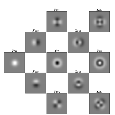
Figure 1: Shapelet basis functions $\chi_{nm}$. The indices “c” and “s” refer to the real part and imaginary part of the complex shapelet basis functions. The FPFS shear estimator combines projections on four shapelet basis functions: $\chi_{00}$, $\chi_{22c}$, $\chi_{22s}$, and $\chi_{40}$. The linear gray color map ranges from $-0.18$ (black) to $0.18$ (white).

In Fourier space, the effect of blurring by a PSF can be removed by dividing $F_{\bm{k}}$ by the PSF’s Fourier power function, $G_{\bm{k}}$ (Zhang, 2008). We decompose the result into shapelets (Massey & Refregier, 2005)

$$M_{nm}=\sum_{\bm{k}}\chi_{nm}^{*}({\bm{k}})\frac{F_{\bm{k}}}{G_{\bm{k}}}\,,$$ (4)

where, to remove a negative sign later, we use complex conjugates of the polar shapelet basis functions (Figure 1)

$$\begin{split}\chi_{nm}(\rho,\phi)&=\frac{(-1)^{(n-|m|)/2}}{r_{F}^{|m|+1}}\left\{\frac{[(n-|m|)/2]!}{\pi[(n+|m|)/2]!}\right\}^{\frac{1}{2}}\\ &\times\rho^{|m|}L^{|m|}_{\frac{n-|m|}{2}}\left(\frac{r^{2}}{r_{F}^{2}}\right)e^{-\rho^{2}/2r_{F}^{2}}e^{-im\phi},\end{split}$$ (5)

where $L^{p}_{q}$ are the Laguerre Polynomials, $n$ is the radial number and $m$ is the spin number, and $r_{F}$ determines the scale of shapelet functions in Fourier space. In addition to ${\bm{k}}$, we use polar coordinates ($\rho$, $\phi$) to denote discrete locations in $2$D Fourier space. The scale size of shapelets used to represent the galaxy, $r_{F}$, should be less than the scale radius of PSF’s Fourier power, $r_{\mathrm{P}}$, to avoid boosting small-scale noise during PSF deconvolution. In this paper, we fix $r_{F}/r_{\mathrm{P}}=0.75$.

To first order in shear, the shear distortion operator correlates a finite number of shapelet modes (separated by $|\Delta n|=2$ and $|\Delta m|=2$ Massey & Refregier 2005). It is therefore possible to estimate an applied shear signal using a finite number of shapelet modes. The Li et al. (2018) FPFS algorithm uses four shapelet modes to construct its shear estimator, with FPFS ‘ellipticity’,

$$e_{1}\equiv\frac{M_{22c}}{M_{00}+C},\qquad e_{2}\equiv\frac{M_{22s}}{M_{00}+C}\,,$$ (6)

where $M_{22c}$ and $M_{22s}$ refer to the real (‘$\cos{}$’) and imaginary (‘$\sin{}$’) components of the complex shapelet mode $M_{22}$ respectively. The positive constant parameter $C$ adjusts the relative weight between galaxies of different luminosities. A large value of $C$ puts more weight on bright galaxies, and suppresses noise bias, while a small value of $C$ weights galaxies more uniformly. We similarly define a few useful spin $m=0$ FPFS quantities:

$$s_{0,2,4}=\frac{M_{00,20,40}}{M_{00}+C}\,.$$ (7)

In principle, the value of $C$ can be different in each of these quantities; however, here we set them all to $2.5\,\sigma_{M_{00}}$ for simplicity, where $\sigma_{M_{00}}$ is the standard deviation of measurement error on $M_{00}$ caused by photon noise on galaxy images. The details of tuning the weighting parameter is shown in Sections 4.1 and 4.2. The ‘flux ratio’ $s_{0}$ was suggested by Li et al. (2018) as a criterion to select a galaxy sample, helping to remove faint galaxies and spurious detections, etc.

When the image of a galaxy is distorted by shear $\gamma_{\beta}$, its ellipticity transforms to first order in $\gamma$ as

$$\bar{e}_{\alpha}\rightarrow{e}_{\alpha}=\bar{e}_{\alpha}+\sum_{\beta=1,2}\gamma_{\beta}(R^{\gamma}_{e})_{\alpha\beta},$$ (8)

where components $\alpha\in\{1,2\}$ and $\beta\in\{1,2\}$, and the ‘shear responsivity’ $(R^{\gamma}_{e})_{\alpha\beta}=\partial e_{\alpha}/\partial\gamma_{\beta}\,$ (Sheldon & Huff, 2017). The shear responsivity of the FPFS ellipticity for an individual galaxy is a scalar quantity,

$$R^{\gamma}_{e}=\frac{1}{\sqrt{2}}\left(s_{4}-s_{0}-e_{1}^{2}-e_{2}^{2}\right),$$ (9)

plus terms involving spin $m=4$ modes — which all average to zero when we now average $R^{\gamma}_{e}$ over all galaxies in a sample, to obtain a population responsivity (denoted with curly letters) $\mathcal{R}^{\gamma}_{e}\equiv\langle R^{\gamma}_{e}\rangle$. We intend to investigate in future work $\mathcal{O}(\gamma^{2})$ terms in $\mathcal{R}^{\gamma}_{e}$ that may not necessarily be small near galaxy clusters. Since the difference between $\langle\bar{e}_{1}^{2}\rangle$ and $\langle\bar{e}_{2}^{2}\rangle$ is negligible, we define the shear response as the average responses of two shear components and do not distinguish between the responses of two shear components.

Assuming that the galaxy population is selected such that $\langle\bar{e}_{\alpha}\rangle=0$ in the absence of shear, equation (8) suggests a shear estimator (Li et al., 2018)

$$\hat{\gamma}_{\alpha}\equiv\frac{\left\langle e_{\alpha}\right\rangle}{\mathcal{R}^{\gamma}_{e}}=\cancelto{0}{\frac{\left\langle\bar{e}_{\alpha}\right\rangle}{\mathcal{R}^{\gamma}_{e}}}+\gamma_{\alpha}=\gamma_{\alpha}\,.$$ (10)

The population variance of $\bar{e}_{\alpha}$ is known as the intrinsic shape noise.

2.2 Nonlinear noise bias

2.2.1 Effect of observational noise

In real observations the galaxy image is contaminated by photon noise and read noise. We denote the total image noise in Fourier space as $n_{\bm{k}}$, i.e. the observed galaxy image is

$$f^{\mathrm{o}}_{\bm{k}}=f_{\bm{k}}+n_{\bm{k}},$$ (11)

and the observed galaxy Fourier power function is

$$F^{\mathrm{o}}_{\bm{k}}=f^{\mathrm{o}}_{\bm{k}}(f^{\mathrm{o}}_{\bm{k}})^{*}=\absolutevalue{f^{\mathrm{o}}_{\bm{k}}}^{2}.$$ (12)

We shall assume that the source and image noise do not correlate, i.e. $\langle f_{\bm{k}}n_{\bm{k}}\rangle=0\,$. We shall also assume that the noise is dominated by background and read noise, so that we can neglect photon noise on the galaxy flux. This makes the noise a mean zero homogeneous Gaussian random field that, averaged over different noise realizations, has Fourier power function with expectation value

$$\mathcal{N}_{\bm{k}}=\left\langle{n}_{\bm{k}}{n}_{\bm{k}}^{*}\right\rangle\,.$$ (13)

Note that this is different from $F_{\bm{k}}$ which is defined for each galaxy, and we differentiate them with different fonts. Using Isserlis’ theorem (also known as Wick’s theorem in quantum field theory), its $4$-point correlation function is

$$\left\langle{n}_{\bm{k}}{n}_{{\bm{k}}^{\prime}}{n}_{\bm{k}}^{*}{n}_{{\bm{k}}^{\prime}}^{*}\right\rangle=\left(1+\operatorname{\delta^{\textsc{k}}}({\bm{k}}-{\bm{k}}^{\prime})+\operatorname{\delta^{\textsc{k}}}({\bm{k}}+{\bm{k}}^{\prime})\right)\mathcal{N}_{\bm{k}}\mathcal{N}_{{\bm{k}}^{\prime}}\,,$$ (14)

where $\operatorname{\delta^{\textsc{k}}}$ denotes the Kronecker delta function.

To account for image noise (following Zhang et al., 2015), the expectation value of the noise power (13) can be measured from blank patches of sky, and subtracted from an observed galaxy’s Fourier power function. Using a tilde to label corrected quantities, this yields​​

$$\tilde{F}_{\bm{k}}=F^{o}_{\bm{k}}-\mathcal{N}_{\bm{k}}\,,$$ (15)

from which $\tilde{e}_{\alpha}$, $\tilde{s}_{0}$, etc. can be defined similarly as in (6), (7), and (4). Note the accent notation of FPFS flux ratio, $s$, follows that of FPFS ellipticity, $e_{1,2}$, shown in Table 1. However, compared to the noiseless image power function $F_{\bm{k}}$, this now contains residual noise power

$${\epsilon}_{\bm{k}}\equiv\tilde{F}_{\bm{k}}-F_{\bm{k}}={n}_{\bm{k}}{n}_{\bm{k}}^{*}-\mathcal{N}_{\bm{k}}+f_{\bm{k}}n_{\bm{k}}^{*}+f_{\bm{k}}^{*}n_{\bm{k}}.$$ (16)

Across a galaxy population, the expectation value of residual noise is zero, $\langle\epsilon_{\bm{k}}\rangle=0$. For any individual galaxy, the residual noise power includes contributions from the individual realisation of noise, and any correlation between that noise and the galaxy flux (see also Li & Zhang, 2021). Combining equations (14) and (16), the two-point correlation function of the residual noise power is

$$\left\langle\epsilon_{\bm{k}}\epsilon^{*}_{{\bm{k}}^{\prime}}\right\rangle=\left(\operatorname{\delta^{\textsc{k}}}({\bm{k}}-{\bm{k}}^{\prime})+\operatorname{\delta^{\textsc{k}}}({\bm{k}}+{\bm{k}}^{\prime})\right)(\mathcal{N}_{\bm{k}}^{2}+2F_{\bm{k}}\mathcal{N}_{\bm{k}})\,.$$ (17)

During shape measurement, the galaxy power function (which now includes residual noise) is divided by the PSF power and decomposed into shapelets (equation 4). The shapelet modes of the residual noise are

$$\mathcal{E}_{nm}=\sum_{\bm{k}}\chi_{nm}^{*}({\bm{k}})\frac{\epsilon_{\bm{k}}}{G_{\bm{k}}}.$$ (18)

Again, their expectation values $\langle\mathcal{E}_{nm}\rangle$ vanish because $\langle\epsilon_{\bm{k}}\rangle=0\,$. For an individual galaxy however, the their covariance is

$$\begin{split}\mathcal{V}_{nmn^{\prime}m^{\prime}}&\equiv\bigl{\langle}\mathcal{E}_{nm}\mathcal{E}^{*}_{n^{\prime}m^{\prime}}\bigr{\rangle}\\ &=\sum_{\bm{k}}\left(\frac{\chi^{*}_{nm}\chi_{n^{\prime}m^{\prime}}+\chi_{nm}\chi_{n^{\prime}m^{\prime}}}{G^{2}_{\bm{k}}}\right)(\mathcal{N}_{\bm{k}}^{2}+2F_{\bm{k}}\mathcal{N}_{\bm{k}})\,.\end{split}$$ (19)

The shapelet modes thus become correlated ($V_{nmn^{\prime}m^{\prime}}\neq 0$) due to inhomogeneous and anisotropic residual noise, and anisotropy in the PSF. The covariances can be measured from nearby blank patches of sky, the galaxy itself, and the PSF model.

2.2.2 Correction for noise bias

Propagating the contribution of residual noise into FPFS ellipticity estimators yields an expectation values

$$\left\langle\tilde{e}_{1}\right\rangle\equiv\left\langle\frac{M_{22c}+\mathcal{E}_{22c}}{M_{00}+C+\mathcal{E}_{00}}\right\rangle, \left\langle\tilde{e}_{2}\right\rangle\equiv\left\langle\frac{M_{22s}+\mathcal{E}_{22s}}{M_{00}+C+\mathcal{E}_{00}}\right\rangle\,.~{}~{}~{}~{}~{}~{}~{}~{}$$ (20)

Expanding the FPFS ellipticity as Taylor series of $\frac{\mathcal{E}_{00}}{M_{00}+C}$ about the point $\mathcal{E}_{00}=0$ and inserting the covariance of shapelet modes (equation (19)), this is

$$\begin{split}\left\langle\tilde{e}_{1}\right\rangle&=\left\langle e_{1}\left(1+\frac{\mathcal{V}_{0000}}{(M_{00}+C)^{2}}\right)-\frac{\mathcal{V}_{0022c}}{(M_{00}+C)^{2}}+O\left(\left(\frac{\mathcal{E}_{nm}}{M_{00}+C}\right)^{4}\right)\right\rangle,\\ \left\langle\tilde{e}_{2}\right\rangle&=\left\langle e_{2}\left(1+\frac{\mathcal{V}_{0000}}{(M_{00}+C)^{2}}\right)-\frac{\mathcal{V}_{0022s}}{(M_{00}+C)^{2}}+O\left(\left(\frac{\mathcal{E}_{nm}}{M_{00}+C}\right)^{4}\right)\right\rangle,\end{split}$$ (21)

where $\mathcal{V}_{0022c}$ ($\mathcal{V}_{0022s}$) refers to the covariance between $\mathcal{E}_{00}$ and $\mathcal{E}_{22c}$ ($\mathcal{E}_{22s}$). One can notice immediately that the second-order terms are in the form of additive and multiplicative biases, proportional to the inverse square of $M_{00}+C\,$. And we shall neglect terms of fourth-order and higher.

Therefore one version of the FPFS ellipticity suitably corrected for noise bias up to second-order is

$$\begin{split}\hat{e}_{1}&=\frac{1}{T}\left(\tilde{e}_{1}+\frac{\mathcal{V}_{0022c}}{(\tilde{M}_{00}+C)^{2}}\right),\\ \hat{e}_{2}&=\frac{1}{T}\left(\tilde{e}_{1}+\frac{\mathcal{V}_{0022s}}{(\tilde{M}_{00}+C)^{2}}\right),\end{split}$$ (22)

where $T=1+\frac{\mathcal{V}_{0000}}{(\tilde{M}_{00}+C)^{2}}\,$. Similarly, the FPFS flux ratio measured from a noisy image, $\tilde{s}_{0}$, is also subject to noise bias, but can be corrected as

$$\hat{s}_{0}=\frac{1}{T}\left(\tilde{s}_{0}+\frac{\mathcal{V}_{0000}}{(\tilde{M}_{00}+C)^{2}}\right).$$ (23)

The corrected shear responsivity for a single, noisy galaxy becomes

$$\hat{R}^{\gamma}_{e}=\frac{1}{\sqrt{2}}\left(\hat{s}_{4}-\hat{s}_{0}-\hat{e}_{1}^{2}-\hat{e}_{2}^{2}\right),$$ (24)

where corrected versions of the other FPFS quantities are listed in Appendix A.

Once again, we average responsivity across a galaxy sample to obtain population response $\hat{\mathcal{R}}^{\gamma}_{e}=\langle\hat{R}^{\gamma}_{e}\rangle$. Assuming that $\langle\bar{e}_{\alpha}\rangle=0$, and now also that $\langle\delta{e}_{\alpha}\rangle=0$, where

$$\delta{e}_{\alpha}\equiv\hat{e}_{\alpha}-e_{\alpha}$$ (25)

is measurement error due to image noise, we obtain a new shear estimator

$$\hat{\gamma}^{\mathrm{A}}_{\alpha}\equiv\frac{\left\langle\hat{e}_{\alpha}\right\rangle}{\hat{\mathcal{R}}^{\gamma}_{e}}=\cancelto{0}{\frac{\left\langle\bar{e}_{\alpha}\right\rangle}{\hat{\mathcal{R}}^{\gamma}_{e}}}+\cancelto{0}{\frac{\left\langle\delta{e}_{\alpha}\right\rangle}{\hat{\mathcal{R}}^{\gamma}_{e}}}+\gamma_{\alpha}=\gamma_{\alpha}$$ (26)

that corrects for nonlinear noise bias to second order. We label this first estimator ‘A’ because we shall next propose more complications. The performance of this shear estimator will be tested in Section 4.1.

2.3 Selection bias

For a complete sample of galaxies, the assumptions that $\langle\bar{e}_{\alpha}\rangle=0$ and $\langle\delta{e}_{\alpha}\rangle=0$ are statistically correct. For an incomplete sample, perhaps restricted to galaxies above a threshold in FPFS flux ratio $\hat{s}_{0}$, this assumption can be broken — creating a shear estimation bias known as selection bias. We correct for the selection bias due to anisotropic intrinsic shape noise, $\langle\bar{e}_{\alpha}\rangle\neq 0$, in Section 2.3.1, and for the seelction bias due to anisotropic measurement error, $\langle\delta{e}_{\alpha}\rangle\neq 0$, in Section 2.3.2.

2.3.1 Selection bias due to anisotropic intrinsic shape noise

Here we derive a correction for the selection bias that is introduced if $\langle\bar{e}_{\alpha}\rangle\neq 0$ in a galaxy population. This can occur if the population is selected according to some quantity that is changed by shear. For example, although unbiased selection could be based upon galaxies’ intrinsic FPFS flux ratios $\bar{s}_{0}$, it would in practice be based upon their lensed flux ratios $s_{0}$. To first order in $\gamma$, these transform under shear as

$$\bar{s}_{0}\rightarrow s_{0}=\bar{s}_{0}+\sum_{\alpha=1,2}\left.\frac{\partial s_{0}}{\partial\gamma_{\alpha}}\right|_{s_{0}=\bar{s}_{0}}\gamma_{\alpha}.$$ (27)

The difference may cause individual galaxies to cross selection thresholds, or to change weight. This effect was first studied in Kaiser (2000) and is referred to as Kaiser flow. In the following discussion, we shall neglect terms $\mathcal{O}(\gamma^{2})$, and temporarily also neglect shape measurement noise.

First consider a complete population of galaxies, whose intrinsic FPFS flux ratio, $\bar{s}_{0}$, and intrinsic ellipticity, $\bar{e}_{\alpha}$ are distributed with probability density function (PDF) $\bar{P}(\bar{s}_{0},\bar{e}_{\alpha})$. Because there is no preferred direction in the Universe, the expectation value of intrinsic galaxy ellipticity $\langle\bar{e}_{\alpha}\rangle=0$.

Next let us identify a subset of the population. In the absence of shear, this can be selected via a cut ${s}_{0}^{\mathrm{low}}<\bar{s}_{0}<{s}_{0}^{\mathrm{upp}}$ between lower and upper bounds on the intrinsic FPFS flux ratio. Because the selection criterion is a spin-$0$ quantity without preferred direction, the expectation value of intrinsic galaxy ellipticity must be preserved​​

$$\left\langle\bar{e}_{\alpha}\right\rangle\Big{|}_{\gamma_{\alpha}=0}=\iint_{s_{0}^{\mathrm{low}}}^{s_{0}^{\mathrm{upp}}}\bar{P}\left(\bar{s},\bar{e}_{\alpha}\right)\bar{e}_{\alpha}~{}\,\mathrm{d}\bar{s}\,\mathrm{d}\bar{e}_{\alpha}=0\,.$$ (28)

However, if a shear has been applied, the selection $\bar{s}_{0}^{\mathrm{low}}<{s}_{0}<\bar{s}_{0}^{\mathrm{upp}}$ must be between limits on lensed quantities

$$\left\langle\bar{e}_{\alpha}\right\rangle=\iint_{s_{0}^{\mathrm{low}}}^{s_{0}^{\mathrm{upp}}}\bar{P}\left(\bar{s},\bar{e}_{\alpha}\right)\bar{e}_{\alpha}~{}\,\mathrm{d}{s}\,\mathrm{d}\bar{e}_{\alpha}\,.$$ (29)

Using equation (27), this selection is equivalent to modified bounds on the intrinsic source plane

$$\left\langle\bar{e}_{\alpha}\right\rangle=\iint_{s_{0}^{\mathrm{low}}-\left.\frac{\partial s_{0}}{\partial\gamma_{\alpha}}\right|_{s_{0}=s_{0}^{\mathrm{low}}}\gamma_{\alpha}}^{s_{0}^{\mathrm{upp}}-\left.\frac{\partial s_{0}}{\partial\gamma_{\alpha}}\right|_{s_{0}=s_{0}^{\mathrm{upp}}}\gamma_{\alpha}}\bar{P}\left(\bar{s},\bar{e}_{\alpha}\right)\bar{e}_{\alpha}~{}\,\mathrm{d}\bar{s}\,\mathrm{d}\bar{e}_{\alpha}\,,$$ (30)

which can have spurious anisotropy $\langle\bar{e}_{\alpha}\rangle\neq 0$. We define the shear response of the galaxy selection on the galaxy sample level, $\mathcal{R}^{\gamma}_{\mathrm{sel}}$, as the ratio between this anisotropy versus the shear that caused it:

$$\begin{split}\mathcal{R}^{\gamma}_{\mathrm{sel}}&\equiv\frac{\langle\bar{e}_{\alpha}\rangle-\langle\bar{e}_{\alpha}\rangle|_{\gamma_{\alpha}=0}}{\gamma_{\alpha}}=\frac{\langle\bar{e}_{\alpha}\rangle}{\gamma_{\alpha}}\\ &=-\bar{P}(s_{0}^{\mathrm{upp}})\left.\left\langle\bar{e}_{\alpha}\frac{\partial s_{0}}{\partial\gamma_{\alpha}}\right\rangle\right|_{s_{0}=s_{0}^{\mathrm{upp}}}+\bar{P}(s_{0}^{\mathrm{low}})\left.\left\langle\bar{e}_{\alpha}\frac{\partial s_{0}}{\partial\gamma_{\alpha}}\right\rangle\right|_{s_{0}=s_{0}^{\mathrm{low}}}\,,\end{split}$$ (31)

where $\bar{P}(s_{0}^{\mathrm{upp}})$ and $\bar{P}(s_{0}^{\mathrm{low}})$ are the marginal probability distributions of $s_{0}$ at $s_{0}^{\mathrm{upp}}$ and $s_{0}^{\mathrm{low}}$, respectively. Those marginal probability distributions can be estimated approximately by the average marginal probability distributions in $[\,s_{0}^{\mathrm{upp}}-0.01\,,s_{0}^{\mathrm{upp}}+0.01\,]$ and $[\,s_{0}^{\mathrm{low}}-0.01\,,s_{0}^{\mathrm{low}}+0.01\,]\,$, respectively. Note that in real observations, we are only able to estimate the marginal probability distributions from noisy, lensed galaxies instead of from noiseless, intrinsic galaxies. We take the assumption that the difference between the intrinsic, noiseless marginal probability distributions and lensed, noisy probability distributions is negligible. Using equation (18) of Li et al. (2018),

$$\left.\left\langle\bar{e}_{\alpha}\frac{\partial s_{0}}{\partial\gamma_{\alpha}}\right\rangle\right|_{s_{0}=s^{\mathrm{low}}_{0}}=\sqrt{2}\left.\left\langle(e_{\alpha}^{2})(1-s_{0})\right\rangle\right|_{s_{0}=s^{\mathrm{low}}_{0}}\,,$$ (32)

we can obtain the shear response of the selection from measurable quantities.

A shear estimator incorporating this selection responsivity

$$\hat{\gamma}^{\mathrm{B}}_{\alpha}\equiv\frac{\left\langle\hat{e}_{\alpha}\right\rangle}{\hat{\mathcal{R}}^{\gamma}_{e}+\mathcal{R}^{\gamma}_{\mathrm{sel}}}=\cancelto{0}{\frac{\left\langle\delta{e}_{\alpha}\right\rangle}{\hat{\mathcal{R}}^{\gamma}_{e}+\mathcal{R}^{\gamma}_{\mathrm{sel}}}}+\frac{\left\langle\bar{e}_{\alpha}\right\rangle}{\hat{\mathcal{R}}^{\gamma}_{e}+\mathcal{R}^{\gamma}_{\mathrm{sel}}}+\frac{\hat{\mathcal{R}}^{\gamma}_{e}~{}\gamma_{\alpha}}{\hat{\mathcal{R}}^{\gamma}_{e}+\mathcal{R}^{\gamma}_{\mathrm{sel}}}=\gamma_{\alpha}$$ (33)

should then be immune to selection bias due to anisotropic intrinsic shape noise. Its performance will be tested on galaxy image simulations in Section 4.3.

2.3.2 Selection bias due to anisotropic measurement error

Here we re-introduce image noise, and derive a correction for the selection bias that is introduced if $\langle\delta{e}_{\alpha}\rangle\neq 0$ in a galaxy population. This can occur if image noise leads to measurement error in a galaxy’s FPFS ellipticity $\delta e_{\alpha}$ that correlates with measurement error in a quantity used for sample selection, e.g. the FPFS flux ratio $\hat{s}_{0}$.

Consider first a population of galaxies with a PDF of noiseless but now lensed quantities $P(e_{\alpha},s_{0})\,$. In this lensed plane, measurement error on the FPFS flux ratio is (c.f. equation (25))

$$\delta{s}_{0}\equiv\hat{s}_{0}-s_{0}\,.$$ (34)

The definitions of $s_{0}$ and $e_{\alpha}$ ensure that, if the image noise is Gaussian, the noise on $s_{0}$ and $e_{\alpha}$ will both be close to Gaussian. In this case, the contribution of image noise to the population variances is

$$\begin{split}\sigma_{s}^{2}&=\langle(\delta{s}_{0})^{2}\rangle\,,\\ \sigma_{e_{\alpha}}^{2}&=\langle(\delta{e}_{\alpha})^{2}\rangle\,,\end{split}$$ (35)

both of which can be estimated from observed galaxy images (see equations (50)) using the covariance of measurement errors on shapelet modes (c.f. equation (19)). The accuracy of the variance estimate will be tested in Section 4.2. Furthermore, the correlation between the measurement errors is

$$\rho_{e_{\alpha}s}=\frac{\langle\delta{e}_{\alpha}\delta{s}_{0}\rangle}{\sigma_{e_{\alpha}}\sigma_{s}},$$ (36)

which can also be estimated from noisy galaxy images (see equations (51)). As indicated by equations (51) and (19), $\rho_{es}\neq 0$ in this lensed plane if either the PSF or the noise power function is anisotropic.

The PDF of noisy lensed quantities can thus be approximated by

$$\hat{P}\simeq P\circledast P^{\delta}$$ (37)

where $\circledast$ refers to the convolution operation and

$$P^{\delta}(e_{\alpha},s_{0})\equiv\frac{1}{2\,\pi\sigma_{s}\sigma_{e_{\alpha}}}\exp\left(-\frac{e_{\alpha}^{2}}{2\,\sigma^{2}_{e_{\alpha}}}-\frac{s_{0}^{2}}{2\,\sigma^{2}_{s}}+\rho_{e_{\alpha}s}\frac{e_{\alpha}s_{0}}{\sigma_{e_{\alpha}}\sigma_{s}}\right)\,.$$ (38)

Convolution with a symmetric kernel $P^{\delta}$ does not shift the centroid of ${P}$, so the average ellipticity of a complete population remains unbiased. However, a cut on FPFS flux ratio $\hat{s}_{0}$ in the presence of noise can bias the average ellipticity such that $\langle\delta{e}_{\alpha}\rangle\neq 0$, if the measurement errors $\delta{e}_{\alpha}$ and $\delta{s}_{0}$ are correlated. The resulting change in ellipticity is

$$e^{\Delta}_{\alpha}\equiv\iint_{s_{0}^{\mathrm{low}}}^{s_{0}^{\mathrm{upp}}}e_{\alpha}\left(\hat{P}-P\right)\,\mathrm{d}e_{\alpha}\,\mathrm{d}s_{0}\,,$$ (39)

which we propose to estimate from measurable quantities

$$\hat{e}^{\Delta}_{\alpha}\simeq\iint_{s_{0}^{\mathrm{low}}}^{s_{0}^{\mathrm{upp}}}e_{\alpha}\left(\hat{P}\circledast P^{\delta}-\hat{P}\right)\,\mathrm{d}e_{\alpha}\,\mathrm{d}s_{0}\,.$$ (40)

For simplicity, we do not recover $P$ by deconvolving $\hat{P}\,$; instead, we take the approximation — $\hat{P}\simeq P\,$.

A final shear estimator correcting for noise bias and both types of selection bias is thus

$$\hat{\gamma}^{\mathrm{C}}_{\alpha}=\frac{\left\langle\hat{e}_{\alpha}\right\rangle-\hat{e}^{\Delta}_{\alpha}}{\hat{\mathcal{R}}^{\gamma}_{e}+\mathcal{R}^{\gamma}_{s}}=\gamma_{\alpha}\,.$$ (41)

The performance of all shear estimators will be tested in Section 4.3.

3 IMAGE SIMULATION

3.1 Galaxies, PSF and noise

We test the FPFS shear estimators by running them on mock astronomical images that have been sheared by a known amount. Our mock data are very similar to sample 2 of Mandelbaum et al. (2018b), replicating the image quality and observing conditions of the Hyper-Suprime Cam (HSC) survey on the 8 m ground-based Subaru telescope, whose deep coadded $i$-band images of the extragalactic sky resolve $\sim$$20$ galaxies per arcminute² brighter than $i=24.5$ (Mandelbaum et al., 2018a; Li et al., 2021). The pixel scale is $0\aas@@fstack{\prime\prime}168\,$.

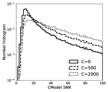
Figure 2: The normalized number histogram as a function of CModel SNR. The histogram is weighted by FPFS ellipticity weight with three different setups, i.e. $C=0$ (solid line), $C=500$ (dashed line) and $C=2000$ (dotted line).

Galaxy images are generated using the open-source package Galsim (Rowe et al., 2015). We randomly select $8\times 10^{4}$ galaxies without repetition from the COSMOS HST Survey catalogue (Leauthaud et al., 2007), which has limiting magnitude $F814W=25.2$. All galaxies have known photometric reshifts. The galaxy shapes are approximated with the best-fitting parametric (de Vaucouleurs 1948 or Sérsic 1963) profile, sheared, convolved with a model of the HSC PSF, then rendered in $64\times 64$ pixel postage stamp images (including a border around the $32\times 32$ pixel region used for shear measurement). The pixel values are finally are multiplied by $2.587$ to rescale the units, so their $i=27$ photometric zeropoint matches that of real HSC pipeline data (Li et al., 2021).

The image PSF is modelled as a Moffat (1969) profile,

$$g_{m}(\mathbf{x})=[1+c(|\mathbf{x}|/r_{\mathrm{P}})^{2}]^{-3.5},$$ (42)

where $c=2^{0.4}-1$ is a constant parameter and $r_{\mathrm{P}}$ is adjusted such that the Full Width Half Maximum (FWHM) of the PSF is $0\aas@@fstack{\prime\prime}6$, matching the mean seeing of the HSC survey (Li et al., 2021). The profile is truncated at a radius four times larger than the FWHM. The PSF is then sheared so that it has ellipticity $(e_{1}=0.02,e_{2}=-0.02)\,$.

We add image noise from a constant sky background and read noise. This includes anisotropic (square-like) correlation between adjacent pixels matching the autocorrelation function of a third-order Lanczos kernel, i.e. $a=3$ in

$$L(x,y)=\begin{cases}\mathrm{sinc}\,(x/a)\,\mathrm{sinc}\,(x)\,\mathrm{sinc}\,(y/a)\,\mathrm{sinc}\,(y)&\mathrm{if}~{}\absolutevalue{x},\absolutevalue{y}<a\\ 0&\mathrm{otherwise,}\end{cases}$$ (43)

where $\mathrm{sinc}\,(x)=\sin{(\pi x)}/\pi x$. This kernel was used to warp and co-add images taken during the first-year HSC survey (Bosch et al., 2018). Ignoring pixel-to-pixel correlations, our resulting noise variance is $7\times 10^{-3}$, which is about two times of the average noise variance in HSC data shown in (Li et al., 2021). In this paper, we do not include photon noise on the galaxy fluxes. This is to increase efficiency because the same realisation of noise can be used in multiple images (see below). However, it means that our tests on the effectiveness of correction for selection bias are an optimistic limit. In Section 4.3 we present tests that bracket the performance achievable if photon noise were to be included.

Our simulated images thus include galaxies with a realistic range of signal-to-noise ratios, SNR, greater than $\sim$10 (Figure 2). We measure a galaxy’s SNR using CModel (Lupton et al., 2001), which fits each image with a linear combination of an exponential and a de Vaucouleurs (de Vaucouleurs, 1948) model, as implemented in the HSC pipeline (Bosch et al., 2018). Writing the FPFS ellipticity as a weighted dimensionless quantity $e_{1}\equiv w\,{M_{22c}}/{M_{00}}$, where $w=(1+C/M_{00})^{-1}$, we find that a value of $C=2000$ reduces the effective contribution of the faintest galaxies by a factor $\sim$3 (dotted line in Figure 2). However, shear measurements from faint galaxies are noisier, and we shall find in Section 4.2 that this weighting also optimises overall SNR.

3.2 Shape noise cancellation

To efficiently reduce intrinsic shape noise in our shear measurements, we generate images of each galaxy in pairs (following Massey et al., 2007), where the intrinsic ellipticity of one is rotated by $90\deg$ (flipping its sign) before applying shear. We then generate three images of each pair with three different shears: ($\gamma_{1}=0.02$, $\gamma_{2}=0$), ($\gamma_{1}=-0.02$, $\gamma_{2}=0$) and ($\gamma_{1}=0$, $\gamma_{2}=0$), but all with exactly the same realisation of image noise (following Pujol et al., 2019; Sheldon et al., 2020). All images are convolved with the same PSF.

To measure the shear measurement bias (equation (1)) of an estimator $\hat{\gamma}$, we calculate

$${c_{1}}=\frac{\langle\hat{e}_{1}^{0}\rangle}{\langle\hat{R}^{\gamma^{0}}_{e}\rangle}$$ (44)

and

$${m_{1}}=\frac{\langle\hat{e}_{1}^{+}-\hat{e}_{1}^{-}\rangle}{0.02\langle\hat{R}^{\gamma+}_{e}+\hat{R}^{\gamma-}_{e}\rangle}-1\,,$$ (45)

where $\hat{e}_{1}^{+}$ and $\hat{R}^{\gamma+}_{e}$ are the first component of ellipticity and shear response estimated from the images with positive shear, $\hat{e}_{1}^{-}$ and $\hat{R}^{\gamma-}_{e}$ from images with negative shear, and $\hat{e}_{1}^{0}$ and $\hat{R}^{\gamma 0}_{e}$ from undistorted images. We repeat this whole process $250$ times with different noise realizations. For these very well-sampled images, we expect the multiplicative bias and additive bias are comparable on component $\hat{\gamma}_{2}\,$.

4 RESULTS

In this section, we test the shear estimators derived in Section 2 using the image simulation described in Section 3. The shear estimators that will be tested include the original Li et al. (2018) shear estimator, $\hat{\gamma}_{\alpha}$ (defined in equation (10)), the shear estimator after correcting the second-order noise bias, $\hat{\gamma}^{\mathrm{A}}_{\alpha}$ (equation (26)), the shear estimator after correcting the selection bias from anisotropic shape noise, $\hat{\gamma}^{\mathrm{B}}_{\alpha}$ (equation (33)), and anisotropic measurement error, $\hat{\gamma}^{\mathrm{C}}_{\alpha}$ (equation (41)). We first test the correction for noise bias in Section 4.1 and the measurement of shape measurement error from noisy galaxy images in Section 4.2. Then we test the correction for selection bias in Section 4.3. Subsequently, we check the redshift dependence of the calibration biases in Section 4.4. Finally, we test the performance of FPFS on poorly resolved galaxies in Section 4.5 and on stellar contamination in Section 4.6.

Note that we force a shear measurement measurement for every simulated galaxy during these tests. For isolated images, the process of source detection influences shear estimation from a population of galaxies, if that population is determined mainly by the selection function of the detector. The right panel of Fig. (3) of Li et al. (2018) showed the $s_{0}$ histograms of detected and undetected galaxies in an HSC-like image simulation Mandelbaum et al. (2018b) — most of the undetected galaxies are clustered at small $s_{0}\,$. Therefore, the influence of the selection function of the detector can be removed by tuning the lower threshold of $s_{0}\,$. For crowded images, removing the bias from detection is challenging since, as shown in Sheldon et al. (2020), the ability of a detection algorithm to recognize blending depends upon the underlying shear distortion.

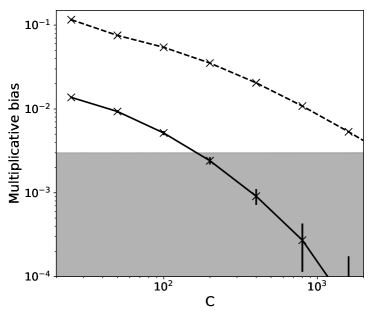
Figure 3: The achieved multiplicative shear measurement bias, as a function of weighting parameter, $C$, both with (solid line) and without (dashed line) the second-order correction for nonlinear noise bias. All measured values of bias are negative, and their absolute values are shown. The gray region denotes the requirement on the control of multiplicative bias for the LSST surveys (The LSST Dark Energy Science Collaboration et al., 2018).

4.1 Nonlinear noise bias

This subsection tests the performance of the second-order noise bias correction derived in Section 2.2. To be more specific, we change the weighting parameter, $C$, and measure the multiplicative bias of our FPFS shear estimator with the second-order noise bias correction, $\hat{\gamma}^{\mathrm{A}}$, using the simulations described in Section 3. The multiplicative bias in Figure 3 is reduced below the requirement for the LSST survey when the weighting parameter is greater than $200$. Since we use all the galaxies in the simulation without any additional selection for the test shown in this subsection, selection bias does not contribute to this result.

We also compare the result of the FPFS shear estimator including the second-order noise bias correction to that of the original FPFS shear estimator without the second-order noise bias correction in Figure 3. As shown, the noise bias is reduced by an order of magnitude after the second-order noise bias correction. The additive bias is constantly below $10^{-4}$, and we do not plot the additive bias here.

Note, the correction of noise bias in Section 2.2 assumes that noise are homogeneous in configuration space so that noise are not correlated in Fourier space. In our simulation described in Section 3, the input noise is homogeneous. In general, the background photon noise is homogeneous in real observations; however the source photon noise is not homogeneous, although its contributions in ground-based surveys are small. In the presence of galaxy source photon noise, the performance of the second-order noise bias correction is expected to be worse than the solid line in Figure 3; however, it should be better than the dashed line Figure 3 that does not include any second-order noise bias correction.

4.2 Shape noise and shape measurement uncertainty

This subsection calculates the statistical uncertainty in shear estimation from a population of galaxies,

$$\sigma_{\gamma}=\frac{\sqrt{\left\langle\,\frac{1}{2}\left(\hat{e}_{1}^{2}+\hat{e}_{2}^{2}\right)\right\rangle}}{\hat{\mathcal{R}}^{\gamma}_{e}}~{}.$$ (46)

This total uncertainty is a combination of noise due to galaxies’ intrinsic shapes, $e_{\text{RMS}}$, and shape measurement error due to realisations of noise in images of galaxies, $\sigma_{e}$. We shall assume these add in quadrature, such that

$$\left\langle\,\frac{1}{2}\left(\hat{e}_{1}^{2}+\hat{e}_{2}^{2}\right)\right\rangle=e_{\text{RMS}}^{2}+\sigma_{e}^{2}\,.$$ (47)

The standard error on the mean shear measured from a population of $N$ galaxies is thus $\sigma_{\gamma}/\sqrt{N}\,$. Note, however, that this value depends on which population of galaxies it is averaged over.

To obtain $e_{\text{RMS}}$, we measure the intrinsic FPFS ellipticity of each galaxy from a realization of the galaxy image simulation with zero noise and zero input shear (see Section 3). We average the two components of ellipticity, then calculate the RMS across our sample of galaxies. The intrinsic shape noise, $e_{\text{RMS}}$, increases with weighting parameter $C$ (dotted line in Figure 4).

To obtain $\sigma_{e}^{2}$, we first measure the total uncertainty using a noisy realization of the galaxy image simulation (see Section 3), again averaging the two components of ellipticity. We then subtract $e_{\text{RMS}}$, following equation (47). The shape measurement error, $\sigma_{e}$, decreases with weighting parameter $C$ (dashed line in Figure 4).

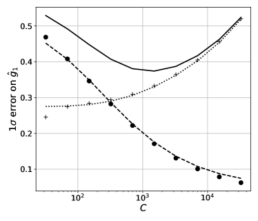
Figure 4: The $1\sigma$ statistical uncertainty on shear measurements $\hat{\gamma}_{1}$ for individual galaxies (solid line), as a function of weighting parameter, $C\,$. The total uncertainty has contributions due to image noise (dashed line) and intrinsic shape noise (dotted line) — both of which we measure using noiseless galaxy images that would not be available to a real survey. However, the ‘$\bullet$’ (‘$+$’) symbols show the same measurement noise (intrinsic shape noise) accurately estimated using equation (35) and noisy galaxy images, which are observable.

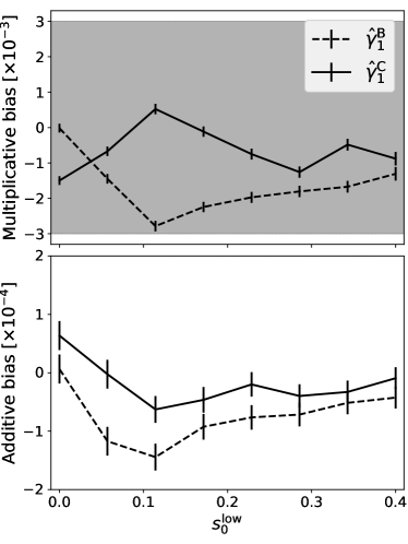
Figure 5: The multiplicative bias (top panel) and additive bias (bottom panel) as a function of lower limit on the FPFS flux ratio. The gray region indicates the LSST science requirement.

The total statistical uncertainty on $\hat{\gamma}_{i}$ is thus a balance between contributions from shape noise (an increasing function of $C\,$) and from measurement error (a decreasing function of $C$). Total uncertainty is minimised for $1000\lesssim C\lesssim 2000$, which is therefore optimal if each galaxy in a sample is equally likely to contain shear signal. In this paper we set $C=2000$ unless otherwise mentioned, which is close to $2.5\,\sigma_{M_{00}}$. The corresponding nonlinear noise bias for this default setup is well below the LSST requirement as shown in Figure 3.

Shape measurement error can be also be estimated independently, using only noisy galaxy images, and without access to noise-free versions – as would be required when handling real astronomical data. Following equation (49), we estimate $\hat{\sigma}_{e}$ (circles in Figure 4), then use measurements of total noise and equation (47) to estimate intrinsic shape noise $\hat{e}_{\text{RMS}}$ (crosses in Figure 4). These reproduce the measurements from noiseless image simulations with remarkable accuracy.

The total FPFS shear measurement uncertainty is similar to that from the calibrated reGauss shear estimator Mandelbaum et al. (2018b). To demonstrate this, we run the HSC pipeline (hscPipe v7) for source detection and shape measurement on our simulated images (see Bosch et al. 2018 for details on the pipeline), which includes catalogue cuts at  $i<24.5$, $\mathrm{resolution}>0.3$, and $\mathrm{SNR}>10$ (Mandelbaum et al., 2018a). To weight the galaxies, we use fixed $C=2000$ for FPFS. For reGauss, we use the optimal weight of a real galaxy in the first-year HSC shear catalogue, selected as the closest match in the $\log\left(\mathrm{SNR}\right)$-$\log\left(\mathrm{resolution}\right)$ plane. Since the reGauss algorithm is subject to certain forms of shear estimation bias (e.g. model bias, noise bias), we also use the reGauss ellipticities measured from the simulation with $\gamma_{1}=0.02$ and $\gamma_{1}=-0.02$ to linearly calibrate its shear response. For this galaxy sample, which has higher S/N than the previous sample, we find shear estimation uncertainty of $\sigma_{\gamma}=0.298$ for FPFS, and $\sigma_{\gamma}=0.288$ for reGauss.

4.3 Selection bias

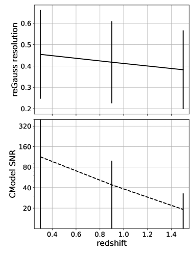
Figure 6: Average reGauss resolution (top panel) and CModel SNR (bottom panel) as functions of redshift. The errorbas show the $1\sigma$ scatter of the corresponding observables in each bin.

This subsection tests the performance of the selection bias correction. Specifically, we adjust the faint-end cut on the FPFS flux ratio, $\hat{s}_{0}>s_{0}^{\mathrm{low}}$, and estimate the shear measurement bias in shear estimators $\hat{\gamma}^{\mathrm{B}}_{\alpha}$ (equation (33)) and $\hat{\gamma}^{\mathrm{C}}_{\alpha}$ (equation (41)). Throughout this section, $s^{\mathrm{upp}}=\infty$, and the weighting parameter is set to $C=2000\,$.

The measured multiplicative biases (top panel of Figure 5) are within the LSST science requirement, for estimators both with ($\hat{\gamma}^{\mathrm{C}}$) and without ($\hat{\gamma}^{\mathrm{B}}$) correction for selection bias due to anisotropic measurement error. Estimator $\hat{\gamma}^{\mathrm{C}}$ improves upon $\hat{\gamma}^{\mathrm{B}}$ by $\sim$$10^{-3}$ on average, which indicates that the multiplicative bias due to anisotropic measurement error is at about this level.

The measured additive biases (bottom panel of Figure 5) are below $1.5\times 10^{-4}$ for $\hat{\gamma}^{\mathrm{B}}$ and below $1\times 10^{-4}$ for $\hat{\gamma}^{\mathrm{C}}$, which indicates that the additive bias due to the anisotropic measurement error is at the level of $10^{-4}\,$.

4.4 Redshift dependence of bias

Figure 7: Shear measurement multiplicative bias (top panel) and additive bias (bottom panel), as a function of galaxy redshift. The gray region indicates the LSST science requirement. Plotted points are offset by $\pm 0.02$ to prevent the error bars from overlapping.

This subsection tests whether the shear measurement biases depend upon galaxy redshift. We divide simulated galaxies into three bins ($0\leq z<0.6$, $0.6\leq z<1.2$, $1.2\leq z<1.8$) according to the photometric redshift of the input COSMOS galaxies (Ilbert et al., 2009). The average reGauss resolution and CModel SNR as functions of redshift are shown in Figure 6.

First, we test shear estimator $\hat{\gamma}^{\mathrm{A}}$ without selecting by any observables other than the COSMOS redshift. Since the COSMOS redshifts are from input galaxies and are not influenced by shear distortion or image noise, the redshift binning does not lead to selection bias. In addition, $\hat{\gamma}^{\mathrm{A}}$ does not account for selection bias; therefore, this test measures any redshift-dependence of the nonlinear noise bias. We find multiplicative bias $|m|<1\times 10^{-3}\,$, and additive bias $|c|<1\times 10^{-4}\,$ at all redshifts (solid lines in Figure 7).

Second, we test shear estimator $\hat{\gamma}^{\mathrm{B}}$ on a galaxy sample selected with $\hat{s}_{0}>s_{0}^{\mathrm{low}}=0.2$. The estimator does not account for the selection bias due to anisotropic measurement error, so this test isolates the performance of its correction for selection bias due to anisotropic shape noise. We find multiplicative bias $|m|\approx 2\times 10^{-3}$ for redshift $z<1$, increasing to $6\times 10^{-3}$ at high redshift $1.2\leq z<1.8$. The additive bias is $2\sigma$ consistent with zero at all redshifts (dashed lines in Figure 7).

Finally, we test shear estimator $\hat{\gamma}^{\mathrm{C}}$ on the same galaxy sample with $\hat{s}_{0}>s_{0}^{\mathrm{low}}=0.2$. This estimator accounts for selection bias due to both anisotropic shape noise and anisotropic measurement error. It produces multiplicative bias consistently $<1\times 10^{-3}$, and additive bias that is $2\sigma$ consistent with zero (dotted lines in Figure 7). Comparing the multiplicative biases of $\hat{\gamma}^{\mathrm{B}}$ and $\hat{\gamma}^{\mathrm{C}}$, we find that the amplitude of the selection bias due to the anisotropic measurement error is a few part in $10^{3}\,$. For these isolated galaxies, our final FPFS shear estimator meets the science requirement of the LSST survey, shown as a gray region in Figure 7.

4.5 Performance with very small source galaxies

Since our fiducial image simulation is based on a training sample of galaxies resolved by HST and with magnitude $i<25.2$, it does not include the smallest galaxies that a future survey might have ambition to measure. To test the accuracy of FPFS on galaxies that are barely resolved (especially by ground-based observations), we use GalSim to simulate small galaxies composed of $20$ points randomly distributed (Zhang et al., 2015) to follow a $2$D Gaussian profile with input half light radius ranging from $0\aas@@fstack{\prime\prime}07$ to $0\aas@@fstack{\prime\prime}2\,$. The flux of each knot is the same. The measured reGauss resolutions range from $0.12$ to $0.27$ as shown in Table 3. Each galaxy sample has $4\times 10^{7}$ galaxies and with an average CModel SNR $\sim 15\,$, and each galaxy is rotated by $45\deg$ four times to reduce shape noise from both spin $m=2$ and spin $m=4$ quantities. Here we do not add any additional selection, so that selection bias is not present. As shown in Table 3, FPFS can accurately measure shear from even extremely small and faint galaxies. If mixed with bigger and brighter galaxies, they will receive a low weight and contribute little to the signal. Crucially, they will not bias it.

Table 3: The average reGauss resolution (first row), shear multiplicative bias (second row), and shear additive bias (third row) for three samples of galaxies simulated as a collection of random point sources. All these galaxies are smaller than those in the HSC shape catalog, which analyses only galaxies with reGauss resolution greater than $0.3$ (Li et al., 2021).

	smallest	smaller	small
reGauss resolution	0.12	0.19	0.27
$m_{1}(10^{-4})$	$0.4\pm 0.9$	$-1.4\pm 0.7$	$-1.0\pm 0.5$
$c_{1}(10^{-4})$	$-2.8\pm 4.5$	$-0.8\pm 1.1$	$-0.5\pm 0.7$

4.6 Stellar contamination

In real observations, stars may not be perfectly removed from the galaxy sample. To test the performance of our FPFS shear estimator with such stellar contamination, we simulate $1\times 10^{7}$ star images with an average SNR $17.8\,$. This corresponds to an extreme situation that the object’s reGauss resolution equals zero. Then we measure the FPFS ellipticity and FPFS response from these stars. Again, we neglect the PSF model errors and assume that we know the two-point correlation function of noise.

Measurements stars yield mean values $\langle\hat{e}_{1}\rangle=(1.0\pm 1.1)\times 10^{-5}$ and $\mathcal{R}_{e}^{\gamma}=(1.8\pm 2.0)\times 10^{-5}$ (Figure 8). That the expectation value of both is consistent with zero (and much smaller than the mean response of simulated HST COSMOS galaxies, $\absolutevalue{\mathcal{R}_{e}^{\gamma}}\sim 0.18$), ensures that FPFS is robust to stellar contamination, so long as the PSF is well determined. Stellar contamination of $n$% will reduce the numerator and denominator of equation (41) by $n$%, leaving the shear estimator unbiased. This is the same good property as METACALIBRATION, demonstrated in Figure 5 of Sheldon & Huff (2017).

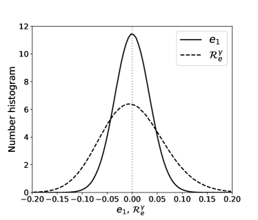
Figure 8: Normalized number histograms of the first component of FPFS ellipticity $e_{1}$ (solid line) and FPFS response $\mathcal{R}_{e}^{\gamma}$ (dashed line) measured from simulated images of stars. The vertical dotted line shows the expectation value.

5 SUMMARY AND OUTLOOK

In this paper, we improve the FPFS weak lensing shear estimator, by implementing corrections for two dominant biases. First, with an assumption that noise in an image is a homogeneous Gaussian random field, we correct for shear measurement noise bias to second order. Second, we derive analytic expressions to remove selection biases due to both anisotropic shape noise and anisotropic measurement error. Crucially, the analytic corrections that we implement in FPFS do not rely upon slow and computationally expensive iterative processes, or upon calibration via external simulations. Our publicly-available code (https://github.com/mr-superonion/FPFS) can process more than a thousand galaxy images per CPU second.

Using mock imaging of isolated SNR$\gtrsim$10 galaxies with known shear, we demonstrate that we have improved the method’s accuracy by an order of magnitude. FPFS now meets the science requirements for a Stage IV weak lensing survey (e.g. Cropper et al., 2013; The LSST Dark Energy Science Collaboration et al., 2018).

Future work should revise this paper’s assumption that galaxies are isolated. Li et al. (2018) and MacCrann et al. (2022) report that the blending of light between neighboring galaxies on the projected plane causes a few percent multiplicative bias for deep ground-based imaging surveys e.g. the HSC Survey (Aihara et al., 2018), DES (DES; Dark Energy Survey Collaboration et al., 2016), and the future LSST. The bias from blending includes shear-dependent blending identification (Sheldon et al., 2020) and bias related to redshift-dependent shear distortion (MacCrann et al., 2022). METADETECTION (Sheldon et al., 2020) is an improved version of METACALIBRATION, able to correct for bias due to shear dependent blending identification. Correction for biases related to blending in FPFS should be the next effect to be tackled. After that, we also intend to explore the use of shapelet modes of order $>2$, which should contain independent information on the shear signal.

DATA AVAILABILITY

The code used for image processing and galaxy image simulation in this paper is available from https://github.com/mr-superonion/FPFS.

Appendix A Second-order revision for nonlinear noise bias

Here we present the expectation values of noisy, measurable quantities (indicated with a tilde), relative to those of the unobservable, noiseless quanties (without a tilde). We only keep to the second-order terms of noise residuals and neglect the higher-order terms. First, we obtain the expectation for $\tilde{s}_{0}$ and $\tilde{s}_{4}$:

$$\begin{split}\left\langle\tilde{s}_{0}\right\rangle&=\left\langle s_{0}\left(1+\frac{\mathcal{V}_{0000}}{(M_{00}+C)^{2}}\right)\right\rangle\\ &-\left\langle\frac{\mathcal{V}_{0000}}{(M_{00}+C)^{2}}\right\rangle,\\ \left\langle\tilde{s}_{4}\right\rangle&=\left\langle s_{4}\left(1+\frac{\mathcal{V}_{0000}}{(M_{00}+C)^{2}}\right)\right\rangle\\ &-\left\langle\frac{\mathcal{V}_{0040}}{(M_{00}+C)^{2}}\right\rangle\,.\end{split}$$ (48)

Then we use the covariance matrix of the shapelet modes (equation (19)) to derive the expectation for $\tilde{e}_{1,2}^{2}$, $\tilde{s}_{0}^{2}$, and $\tilde{e}_{1,2}\tilde{s}_{0}$:

$$\begin{split}\left\langle\tilde{e}_{1}^{2}\right\rangle&=\left\langle e_{1}^{2}\left(1+3\frac{\mathcal{V}_{0000}}{(M_{00}+C)^{2}}\right)\right\rangle\\ &+\left\langle\frac{\mathcal{V}_{22c22c}}{(M_{00}+C)^{2}}-4e_{1}\frac{\mathcal{V}_{0022c}}{(M_{00}+C)^{2}}\right\rangle,\\ \left\langle\tilde{e}_{2}^{2}\right\rangle&=\left\langle e_{2}^{2}\left(1+3\frac{\mathcal{V}_{0000}}{(M_{00}+C)^{2}}\right)\right\rangle\\ &+\left\langle\frac{\mathcal{V}_{22s22s}}{(M_{00}+C)^{2}}-4e_{2}\frac{\mathcal{V}_{0022s}}{(M_{00}+C)^{2}}\right\rangle,\\ \left\langle\tilde{s}_{0}^{2}\right\rangle&=\left\langle s_{0}^{2}\left(1+3\frac{\mathcal{V}_{0000}}{(M_{00}+C)^{2}}\right)\right\rangle\\ &+\left\langle\frac{\mathcal{V}_{0000}}{(M_{00}+C)^{2}}-4s_{0}\frac{\mathcal{V}_{0000}}{(M_{00}+C)^{2}}\right\rangle,\\ \left\langle\tilde{e}_{1}\tilde{s}_{0}\right\rangle&=\left\langle e_{1}s_{0}\left(1+3\frac{\mathcal{V}_{0000}}{(M_{00}+C)^{2}}\right)\right\rangle\\ &+\left\langle\frac{\mathcal{V}_{0022c}}{(M_{00}+C)^{2}}-2s_{0}\frac{\mathcal{V}_{0022c}}{(M_{00}+C)^{2}}\right\rangle\\ &-\left\langle 2e_{1}\frac{\mathcal{V}_{0000}}{(M_{00}+C)^{2}}\right\rangle,\\ \left\langle\tilde{e}_{2}\tilde{s}_{0}\right\rangle&=\left\langle e_{2}s_{0}\left(1+3\frac{\mathcal{V}_{0000}}{(M_{00}+C)^{2}}\right)\right\rangle\\ &+\left\langle\frac{\mathcal{V}_{0022s}}{(M_{00}+C)^{2}}-2s_{0}\frac{\mathcal{V}_{0022s}}{(M_{00}+C)^{2}}\right\rangle\\ &-\left\langle 2e_{2}\frac{\mathcal{V}_{0000}}{(M_{00}+C)^{2}}\right\rangle\,.\end{split}$$ (49)

These quantities are used to derive the variance of measurement error on FPFS ellipticity $\delta{e}_{1,2}$ defined in equation (25) and flux ratio $\delta{s}_{0}$ defined in equation (34) due to the photon noise on galaxy images where noise terms of fourth order and higher are neglected.

$$\begin{split}\langle(\delta{e}_{1})^{2}\rangle&=\left\langle\hat{e}_{1}^{2}-e_{1}^{2}\right\rangle\\ &=\left\langle\tilde{e}_{1}^{2}\,\frac{\mathcal{V}_{0000}}{(\tilde{M}_{00}+C)^{2}}+\frac{\mathcal{V}_{22c22c}}{(\tilde{M}_{00}+C)^{2}}-2\,\tilde{e}_{1}\,\frac{\mathcal{V}_{0022c}}{(\tilde{M}_{00}+C)^{2}}\right\rangle\,,\\ \langle(\delta{e}_{2})^{2}\rangle&=\left\langle\hat{e}_{2}^{2}-e_{2}^{2}\right\rangle\\ &=\left\langle\tilde{e}_{2}^{2}\,\frac{\mathcal{V}_{0000}}{(\tilde{M}_{00}+C)^{2}}+\frac{\mathcal{V}_{22s22s}}{(\tilde{M}_{00}+C)^{2}}-2\,\tilde{e}_{2}\,\frac{\mathcal{V}_{0022s}}{(\tilde{M}_{00}+C)^{2}}\right\rangle\,,\\ \langle(\delta{s}_{0})^{2}\rangle&=\left\langle\hat{s}_{0}^{2}-s_{0}^{2}\right\rangle\\ &=\left\langle\tilde{s}_{0}^{2}\frac{\mathcal{V}_{0000}}{(\tilde{M}_{00}+C)^{2}}+\frac{\mathcal{V}_{0000}}{(\tilde{M}_{00}+C)^{2}}-2\,\tilde{s}_{0}\,\frac{\mathcal{V}_{0000}}{(\tilde{M}_{00}+C)^{2}}\right\rangle\,.\\ \end{split}$$ (50)

In addition, the correlation between the measurement errors $\delta{e}_{1,2}$ and $\delta{s}_{0}$ is given by

$$\begin{split}\langle\delta{s}_{0}\delta{e}_{1}\rangle&=\left\langle\hat{s}_{0}\hat{e}_{1}-s_{0}e_{1}\right\rangle\\ &=\left\langle\tilde{e}_{1}\tilde{s}_{0}\frac{\mathcal{V}_{0000}}{(\tilde{M}_{00}+C)^{2}}+\frac{\mathcal{V}_{0022c}}{(\tilde{M}_{00}+C)^{2}}\right\rangle\\ &-\left\langle\tilde{s}_{0}\,\frac{\mathcal{V}_{0022c}}{(\tilde{M}_{00}+C)^{2}}+\tilde{e}_{1}\,\frac{\mathcal{V}_{0000}}{(\tilde{M}_{00}+C)^{2}}\right\rangle,\\ \langle\delta{s}_{0}\delta{e}_{2}\rangle&=\left\langle\hat{s}_{0}\hat{e}_{2}-s_{0}e_{2}\right\rangle\\ &=\left\langle\tilde{e}_{2}\tilde{s}_{0}\frac{\mathcal{V}_{0000}}{(\tilde{M}_{00}+C)^{2}}+\frac{\mathcal{V}_{0022s}}{(\tilde{M}_{00}+C)^{2}}\right\rangle\\ &-\left\langle\tilde{s}_{0}\,\frac{\mathcal{V}_{0022s}}{(\tilde{M}_{00}+C)^{2}}+\tilde{e}_{2}\,\frac{\mathcal{V}_{0000}}{(\tilde{M}_{00}+C)^{2}}\right\rangle,\\ \end{split}$$ (51)

Finally we derive expectation for the noisy quantities related to the selection shear response:

$$\begin{split}\left\langle(\tilde{e}_{1})^{2}\tilde{s}_{0}\right\rangle&=\left\langle(e_{1})^{2}s_{0}\left(1+6\frac{\mathcal{V}_{0000}}{(M_{00}+C)^{2}}\right)\right\rangle\\ &-3\left\langle(e_{1})^{2}\frac{\mathcal{V}_{0000}}{(M_{00}+C)^{2}}\right\rangle+\left\langle s_{0}\frac{\mathcal{V}_{22c22c}}{(M_{00}+C)^{2}}\right\rangle\\ &+\left\langle 2e_{1}\left(1-3s_{0}\right)\frac{\mathcal{V}_{0022c}}{(M_{00}+C)^{2}}\right\rangle,\\ \left\langle(\tilde{e}_{2})^{2}\tilde{s}_{0}\right\rangle&=\left\langle(e_{2})^{2}s_{0}\left(1+6\frac{\mathcal{V}_{0000}}{(M_{00}+C)^{2}}\right)\right\rangle\\ &-3\left\langle(e_{2})^{2}\frac{\mathcal{V}_{0000}}{(M_{00}+C)^{2}}\right\rangle+\left\langle s_{0}\frac{\mathcal{V}_{22s22s}}{(M_{00}+C)^{2}}\right\rangle\\ &+\left\langle 2e_{2}\left(1-3s_{0}\right)\frac{\mathcal{V}_{0022s}}{(M_{00}+C)^{2}}\right\rangle\,.\\ \end{split}$$ (52)

References

- Aihara et al. (2018) Aihara H., et al., 2018, PASJ, 70, S8
- Bartelmann & Schneider (2001) Bartelmann M., Schneider P., 2001, Physics Reports, 340, 291
- Bernstein (2010) Bernstein G. M., 2010, MNRAS, 406, 2793
- Bernstein & Armstrong (2014) Bernstein G. M., Armstrong R., 2014, MNRAS, 438, 1880
- Bernstein et al. (2016) Bernstein G. M., Armstrong R., Krawiec C., March M. C., 2016, MNRAS, 459, 4467
- Bosch et al. (2018) Bosch J., et al., 2018, PASJ, 70, S5
- Cropper et al. (2013) Cropper M., et al., 2013, MNRAS, 431, 3103
- Dark Energy Survey Collaboration et al. (2016) Dark Energy Survey Collaboration et al., 2016, MNRAS, 460, 1270
- Fenech Conti et al. (2017) Fenech Conti I., Herbonnet R., Hoekstra H., Merten J., Miller L., Viola M., 2017, MNRAS, 467, 1627
- Hirata & Seljak (2003) Hirata C., Seljak U., 2003, MNRAS, 343, 459
- Hoekstra (2021) Hoekstra H., 2021, A&A, 656, A135
- Huff & Mandelbaum (2017) Huff E., Mandelbaum R., 2017, preprint, (arXiv:1702.02600)
- Ilbert et al. (2009) Ilbert O., et al., 2009, ApJ, 690, 1236
- Ivezić et al. (2019) Ivezić Ž., et al., 2019, ApJ, 873, 111
- Kaiser (2000) Kaiser N., 2000, The Astrophysical Journal, 537, 555
- Kannawadi et al. (2019) Kannawadi A., et al., 2019, A&A, 624, A92
- Kilbinger (2015) Kilbinger M., 2015, Reports on Progress in Physics, 78, 086901
- Laureijs et al. (2011) Laureijs R., et al., 2011, preprint, (arXiv:1110.3193)
- Leauthaud et al. (2007) Leauthaud A., et al., 2007, ApJS, 172, 219
- Li & Zhang (2021) Li H., Zhang J., 2021, ApJ, 911, 115
- Li et al. (2018) Li X., Katayama N., Oguri M., More S., 2018, MNRAS, 481, 4445
- Li et al. (2021) Li X., et al., 2021, preprint, (arXiv:2107.00136)
- Lupton et al. (2001) Lupton R., Gunn J. E., Ivezić Z., Knapp G. R., Kent S., 2001, in Harnden F. R. J., Primini F. A., Payne H. E., eds, Astronomical Society of the Pacific Conference Series Vol. 238, Astronomical Data Analysis Software and Systems X. p. 269 (arXiv:astro-ph/0101420)
- MacCrann et al. (2022) MacCrann N., et al., 2022, MNRAS, 509, 3371
- Mandelbaum (2018) Mandelbaum R., 2018, ARA&A, 56, 393
- Mandelbaum et al. (2018a) Mandelbaum R., et al., 2018a, PASJ, 70, S25
- Mandelbaum et al. (2018b) Mandelbaum R., et al., 2018b, MNRAS, 481, 3170
- Massey & Refregier (2005) Massey R., Refregier A., 2005, MNRAS, 363, 197
- Massey et al. (2007) Massey R., et al., 2007, MNRAS, 376, 13
- Massey et al. (2010) Massey R., Kitching T., Richard J., 2010, Reports on Progress in Physics, 73, 086901
- Massey et al. (2013) Massey R., et al., 2013, MNRAS, 429, 661
- Miller et al. (2007) Miller L., Kitching T. D., Heymans C., Heavens A. F., Van Waerbeke L., 2007, Monthly Notices of the Royal Astronomical Society, 382, 315
- Moffat (1969) Moffat A. F. J., 1969, A&A, 3, 455
- Pujol et al. (2019) Pujol A., Kilbinger M., Sureau F., Bobin J., 2019, A&A, 621, A2
- Refregier (2003) Refregier A., 2003, MNRAS, 338, 35
- Refregier et al. (2012) Refregier A., Kacprzak T., Amara A., Bridle S., Rowe B., 2012, MNRAS, 425, 1951
- Rowe et al. (2015) Rowe B. T. P., et al., 2015, Astronomy and Computing, 10, 121
- Sérsic (1963) Sérsic J. L., 1963, Boletin de la Asociacion Argentina de Astronomia La Plata Argentina, 6, 41
- Sheldon & Huff (2017) Sheldon E. S., Huff E. M., 2017, ApJ, 841, 24
- Sheldon et al. (2020) Sheldon E. S., Becker M. R., MacCrann N., Jarvis M., 2020, ApJ, 902, 138
- Spergel et al. (2015) Spergel D., et al., 2015, preprint, (arXiv:1503.03757)
- The LSST Dark Energy Science Collaboration et al. (2018) The LSST Dark Energy Science Collaboration et al., 2018, arXiv e-prints, p. arXiv:1809.01669
- Zhang (2008) Zhang J., 2008, MNRAS, 383, 113
- Zhang et al. (2015) Zhang J., Luo W., Foucaud S., 2015, JCAP, 1, 24
- Zhang et al. (2017) Zhang J., Zhang P., Luo W., 2017, ApJ, 834, 8
- de Vaucouleurs (1948) de Vaucouleurs G., 1948, Annales d’Astrophysique, 11, 247