FM-Indexing Grammars Induced by Suffix Sorting for Long Patterns

Abstract

The run-length compressed Burrows-Wheeler transform (RLBWT) used in conjunction with the backward search introduced in the FM index is the centerpiece of most compressed indexes working on highly-repetitive data sets like biological sequences. Compared to grammar indexes, the size of the RLBWT is often much bigger, but queries like counting the occurrences of long patterns can be done much faster than on any existing grammar index so far. In this paper, we combine the virtues of a grammar with the RLBWT by building the RLBWT on top of a special grammar based on induced suffix sorting. Our experiments reveal that our hybrid approach outperforms the classic RLBWT with respect to the index sizes, and with respect to query times on biological data sets for sufficiently long patterns.

1 Introduction

A text index built on a string $T$ of length $n$ is a data structure that can answer the following queries, for a given pattern $P$ of length $m$:

exists(P)

: does the pattern $P$ occur in $T$?

count(P)

: how often does the pattern $P$ occur in $T$?

locate(P)

: where does the pattern $P$ occur in $T$?

The answers are a boolean, a number, and a list of starting positions in the text, respectively. ${{\textrm{{locate}}}}(P)$ is the most powerful query because the cardinality of its returned set is the return value of ${{\textrm{{count}}}}(P)$, whereas ${{\textrm{{count}}}}(P)>0$ is a boolean statement equivalent to ${{\textrm{{exists}}}}(P)$.

One prominent example of such a text index is the FM-index [15]. It consists of a wavelet tree [22] built upon the BWT [5] of the text, and can answer ${{\textrm{{count}}}}(P)$ in time linear to the length of $P$ multiplied by the operational cost of the wavelet tree, which can be logarithmic in the alphabet size and up to constant [3]. Given the BWT consists of $r$ maximal character runs, this data structure can be represented by two additional bit vectors [29, Thm. 3] of length $n$ in $r\lg\sigma+\mathop{}\mathopen{}o\mathopen{}(r\lg\sigma)+\mathop{}\mathopen{}\mathcal{O}\mathopen{}(n)$ bits of space. This space can be further reduced with Huffman-shaped wavelet trees by exploiting the zeroth order empirical entropy on the string consisting of the different letters of the runs in the BWT. For locate, the indexes based on the BWT are augmented by a sampling of the suffix array [30], which needs $n\lg n$ bits in its plain form. In what follows, we do not address locate since this augmentation can be done orthogonal to our proposed data structure, and is left as future work.

Although current approaches achieve $\mathop{}\mathopen{}\mathcal{O}\mathopen{}(m)$ time for ${{\textrm{{count}}}}(P)$ with $|P|=m$, it involves $\mathop{}\mathopen{}\mathcal{O}\mathopen{}(m)$ queries to the underlying wavelet tree data structure, which is performed in a constant number of random accesses. Unfortunately, these random accesses make the FM-index rather slow in practice. The BWT built on a grammar compressed string allows us to match non-terminals in one backward search step, hence allowing us to jump over multiple characters in one step. Consequently, we spend less time on the cache-unfriendly wavelet tree, but more time on extracting the grammar symbols stored in cache-friendly arrays. Our experiments reveal that this extra work pays off for the reduced usage of the wavelet tree regarding the time performance. Regarding the space, the grammar captures the compressibility far better than the run-length compression of the BWT built on the plain text. Here, we leverage certain properties of the GCIS (grammar compression by induced suffix sorting) grammar [36], which have been discovered by Akagi et al. [1] and Díaz-Domínguez et al. [14] for determining non-terminals of the text matching portions of the pattern.

Our Contribution

To sum up, our contribution is that combining the BWT with a specific choice of grammar-based compression method achieves potentially better compression than the plain RLBWT, and at the same time reducing the memory accesses for count queries (heuristically). This comes at the expense of additional computation for building the grammar of the text during the construction and of the pattern during a query.

Related Work

A lot of research effort has been invested in analyzing and improving count of the BWT (e.g., [29] and the references therein) and the sampling of the suffix array (e.g., [18] and the references therein). Another line of research are grammar indexes, which usually enhance a grammar for locate queries. Although computing the smallest grammar is NP-complete [6], there are grammars with a size of $\mathop{}\mathopen{}\mathcal{O}\mathopen{}(r\log(n/r))$ [18], and some grammars are empirically much smaller than the RLBWT in practice. However, most indexes have a quadratic dependency on the pattern length for locate [9, 10], and are unable to give improved query times independent of the number of occurrences of the pattern, when considering only count. A novel exception is the grammar index of Christiansen et al. [7], which achieves $\mathop{}\mathopen{}\mathcal{O}\mathopen{}(m+\log^{2+\epsilon}n)$ time for count with a space of $\mathop{}\mathopen{}\mathcal{O}\mathopen{}(\gamma\log(n/\gamma))$, for $\gamma$ being the size of the smallest string attractor [26] of the input text. However, this approach seems to be rather impractical, and up to now nobody has considered implementing it. Related to our work is the grammar indexes of Akagi et al. [1] and Díaz-Domínguez et al. [14], which are also based on the GCIS grammar, where the latter is based on results of Christiansen et al. [7]. They also use similar techniques for extracting non-terminals from the pattern grammar, for which they can be sure of that these appear in the text grammar. However, they need to call locate for computing count, and thus their time complexity is dependent on the number of occurrences of a pattern.

We are not aware of a combination of the BWT with grammar techniques, except for construction. Here, Kärkkäinen et al. [24] studied the construction of the BWT upon a grammar-compressed input. They applied a grammar compression merging frequent bigrams similar to Re-Pair [28], and empirically could improve the computation of the BWT as well as the reconstruction of the text from the BWT. With a similar target, Díaz-Domínguez and Navarro [13], Díaz-Domínguez and Navarro [12] computed the extended BWT [31], a BWT variant for multiple texts, from the GCIS grammar.

2 Preliminaries

With $\lg$ we denote the logarithm to base two (i.e., $\lg=\log_{2}$). Our computational model is the word RAM with machine word size $\mathop{}\mathopen{}\mathup{\Omega}\mathopen{}(\lg n)$, where $n$ denotes the length of a given input string $T[1..n]$, which we call the text, whose characters are drawn from an integer alphabet $\Sigma=\{1,\ldots,\sigma\}$ of size $\sigma=n^{\mathop{}\mathopen{}\mathcal{O}\mathopen{}(1)}$. We call the elements of $\Sigma$ characters. A character run is a maximal substring consisting of repetition of the same character. For a string $S\in\Sigma^{*}$, we denote with $S[i..]$ its $i$-th suffix, and with $|S|$ its length. Given $X,Y,Z\in\Sigma^{*}$ with $S=XYZ$, then $X$, $Y$ and $Z$ are called a prefix, substring and suffix of $S$, respectively. We say that a prefix $X$ (resp. suffix $Z$) is proper if $X\not=S$ (resp. $Z\not=S$). The order $<$ on the alphabet $\Sigma$ induces a lexicographic order on $\Sigma^{*}$, which we denote by $\prec$.

Given a character $\texttt{c}\in\Sigma$, and an integer $j$, the rank query $T.\operatorname{rank}_{\texttt{c}}(j)$ counts the occurrences of c in $T[1..j]$, and the select query $T.\operatorname{select}_{\texttt{c}}(j)$ gives the position of the $j$-th c in $T$. We stipulate that $\operatorname{rank}_{\texttt{c}}(0)=\operatorname{select}_{\texttt{c}}(0)=0$. If the alphabet is binary, i.e., when $T$ is a bit vector, there are data structures [23, 8] that use $\mathop{}\mathopen{}o\mathopen{}(|T|)$ extra bits of space, and can compute $\operatorname{rank}{}$ and $\operatorname{select}{}$ in constant time, respectively. Each of those data structures can be constructed in time linear in $|T|$. We say that a bit vector has a rank-support and a select-support if it is endowed by data structures providing constant time access to $\operatorname{rank}$ and $\operatorname{select}$, respectively.

2.1 Burrows-Wheeler Transform

The BWT of $T$ is a permutation of the characters of $\tilde{T}:=T\texttt{\$}$, where we appended an artificial character $ smaller than all characters appearing in $T$. This BWT, denoted by $\mathsf{BWT}$, is defined such that $\mathsf{BWT}[i]$ is the preceding character of $\tilde{T}$’s $i$-th lexicographically smallest suffix, or $\tilde{T}[|\tilde{T}|]=\texttt{\$}$ in case that this suffix is $\tilde{T}$ itself. Given a pattern $P[1..m]$, the range of $P[i..m]$ in $\mathsf{BWT}$ is an interval $[\ell_{i}..r_{i}]$ such that $\tilde{T}[j..]$ has $P[i..m]$ as a prefix if and only if $\tilde{T}[j..]$ is the $k$-th lexicographically smallest suffix with $k\in[\ell_{i}..r_{i}]$. The range $[\ell_{i},r_{i}]$ of $P[i..m]$ can be computed from $P[i+1..m]$ by a backward search step on $\mathsf{BWT}$ with an array $C[1..\sigma]$, where $C[c]$ is the number of occurrences of those characters in $\mathsf{BWT}$ that are smaller than $c$, for $c\in[1..\sigma]$. Given the range of $P[i+1..m]$ is $[\ell_{i+1}..r_{i+1}]$, $\ell_{i}$ and $r_{i}$ are determined by $\ell_{i}=C[P[i]]+\mathsf{BWT}.\operatorname{rank}_{P[i]}(\ell_{i+1}+1)$ and $r_{i}=C[P[i]]+\mathsf{BWT}.\operatorname{rank}_{P[i]}(r_{i+1})$, with $\ell_{m}=C[P[m]]+1$ and $r_{m}=C[P[m]+1]$. We focus on ranges since the length of the range of $P$ is ${{\textrm{{count}}}}(P)$.

Example for BWT ranges

Given the text from Table 1, and a pattern $P[1..6]=\texttt{cabaca}$, then the range of $P[6]=\texttt{a}$ is $[2..6]$, and the range of $P[5..6]=\texttt{ca}$ is $[12..13]$ since the c’s contained in the previous range $\mathsf{BWT}[2..6]$ are the second and third c in $\mathsf{BWT}$, which are in $F$ at positions $12$ and $13$, where $F[i]=\mathop{\text{argmin}}_{c\in\Sigma}\{C[c]:i\leq C[c]\}$ is the $i$-th lexicographically smallest character in $\mathsf{BWT}$.

Table 1: BWT and array $F$ of $T:=\texttt{bacabacaacbcbc\$}$.

$i$	1	2	3	4	5	6	7	8	9	10	11	12	13	14	15
$F[i]$	$	a	a	a	a	a	b	b	b	b	c	c	c	c	c
$\mathsf{BWT}[i]$	c	c	c	b	b	a	a	$	c	c	b	a	a	b	a

2.2 Grammars

An admissible (context-free) grammar [27] built upon a string $T\in\Sigma^{*}$ is a tuple $\mathcal{G}_{T}:=(\Gamma,\pi,X_{T})$ with $\Gamma$ being the set of non-terminals, a function $\pi:\Gamma\rightarrow(\Sigma\cup\Gamma)^{+}$ that applies (production) rules, and a start symbol $X_{T}$ such that the iterative application of $\pi$ on $X_{T}$ eventually gives $T$. Additionally, $\pi$ is injective, there is no $X\in\Gamma$ with $|\pi(X)|=0$, and for each $X\in\Gamma\setminus\{X_{T}\}$, there is a $Y\in\Gamma$ such that $X$ is contained in $\pi(Y)$. Obviously, $\mathcal{G}_{T}$ has no cycle.

For simplicity, we stipulate that $\pi(c)=c$ for $c\in\Sigma$. We say that a non-terminal ($\in\Gamma$) or a character ($\in\Sigma$) is a symbol, and denote the set of characters and non-terminals with $\mathcal{S}:=\Sigma\cup\Gamma$. We understand $\pi$ also as a string morphism $\pi:\mathcal{S}^{*}\rightarrow\mathcal{S}^{*}$ by applying $\pi$ on each symbol of the input string. This allows us to define the expansion $\pi^{*}(X)$ of a symbol $X$, which is the iterative application of $\pi$ until obtaining a string of characters, i.e., $\pi^{*}(X)\subset\Sigma^{*}$ and $\pi^{*}(X_{T})=T$. Since $\pi(X)$ is deterministically defined, we use to say the right hand side of $X$ for $\pi(X)$. The lexicographic order on $\Sigma$ induces an ordering on $\Gamma$ by saying that $X\prec Y$ if and only if $\pi^{*}(X)\prec\pi^{*}(Y)$.

Further, we call an admissible grammar factorizing if we can split $\Gamma$ into the sets ${\Sigma}^{(1)},\ldots,{\Sigma}^{(t_{T})}$ such that ${\Sigma}^{(t_{T})}=\{X_{T}\}$, and $\pi:{\Sigma}^{(h)}\rightarrow{\Sigma}^{(h-1)}$ with ${\Sigma}^{(0)}=\Sigma$ is well-defined for each $h\in[1..t_{T}]$. In particular, ${\pi}^{(t_{T})}(X_{T})=T$. We say that $\mathcal{G}_{T}$ has the height $t_{T}$, and that ${\Sigma}^{(h)}$ are the non-terminals on height $h$. We write ${T}^{(h)}={\pi}^{(t_{T}-h)}(X_{T})$ with ${T}^{(0)}=T$, and ${\sigma}^{(h)}:=|{\Sigma}^{(h)}|$ for $h\geq 0$. Examples for factorizing grammars are ESP [11] and HSP [17], but not Re-Pair [28] or sequitur [34] in general. Another example is GCIS, which we review next.

2.3 Grammar Compression Based on Induced Suffix Sorting

SAIS [35] is a linear-time algorithm for computing the suffix array [30]. We briefly sketch the parts of SAIS needed for constructing the GCIS grammar. Starting with a text $T[1..n]$, we pad it with artificial characters # and $ to its left and right ends, respectively, such that $T[0]=\texttt{\#}$ and $T[n+1]=\texttt{\$}$. We stipulate that $\texttt{\#}<\texttt{\$}<c$ for each character $c\in\Sigma$. Central to SAIS is the type assignment to each suffix, which is either L or S:

• $T[i..]$ is an L suffix if $T[i..]\succ T[i+1..]$, or

• $T[i..]$ is an S suffix otherwise, i.e., $T[i..]\prec T[i+1..]$,

where we stipulate that $T[n+1]=\texttt{\$}$ is always type S. Since it is not possible that $T[i..]=T[i+1..]$, SAIS assigns each suffix a type. An S suffix $T[i..]$ is additionally an $\texttt{S}^{*}$ suffix if $T[i-1..]$ is an L suffix. Note that $T[0..]$ is an S suffix since # is the smallest character; we further let it be $\texttt{S}^{*}$. The substring between two succeeding $\texttt{S}^{*}$ suffixes is called an LMS substring. In other words, a substring $T[i..j]$ with $i<j$ is an LMS substring if and only if $T[i..]$ and $T[j..]$ are $\texttt{S}^{*}$ suffixes and there is no $k\in[i+1..j-1]$ such that $T[k..]$ is an $\texttt{S}^{*}$ suffix.

The LMS substrings induce a factorization of $T[0..n+1]=T_{1}\cdots T_{t}$, where each factor starts with an LMS substring. We call this factorization LMS factorization. By replacing each factor $T_{x}$ by the lexicographic rank of its respective LMS substring, we obtain a string ${T}^{(1)}$ of these ranks. We recurse on ${T}^{(1)}$ until we obtain a string ${T}^{(t_{T}-1)}$ whose rank-characters are all unique or whose LMS factorization consists of at most two factors. If we, instead of assigning ranks, assign each LMS substring a non-terminal, and recurse on a string of non-terminals, we obtain a grammar $\mathcal{G}_{T}$ that is factorizing. Specifically, the right hand side of a non-terminal is an LMS substring without its last character, and the special characters # and $ are omitted. The start symbol is defined by $X_{T}\rightarrow{T}^{(t_{T})}$.

Lemma 2.1 ([36]).

The GCIS grammar $\mathcal{G}_{T}$ can be constructed in $\mathop{}\mathopen{}\mathcal{O}\mathopen{}(n)$ time. $\mathcal{G}_{T}$ is reduced, meaning that we can reach all non-terminals of $\Gamma$ from ${X}^{(t_{T})}$.

Since there are no neighboring $\texttt{S}^{*}$ suffixes, an LMS substring has a length of at least three, and therefore the right-hand sides of all non-terminals are of length at least two (except maybe for the first factor). This means that the length of ${T}^{(i)}$ is at most half of the length of ${T}^{(i-1)}$ for $i\geq 1$. Consequently, the height $t_{T}$ is $\mathop{}\mathopen{}\mathcal{O}\mathopen{}(\lg n)$.

2.4 Example for a GCIS grammar

We build GCIS on the example text $T:=\texttt{bacabacaacbcbc}$. For that, we determine the types of all suffixes, which determine the LMS substrings, as shown in Fig. 1.

Figure 1: Application of GCIS on the text $T:=\texttt{bacabacaacbcbc}$. The type of each suffix is shown below its starting position. The rectangular bracket below the types demarcate the LMS substrings.

We obtain the grammar $\mathcal{G}_{T}$ with the following rules: $\texttt{A}\rightarrow\texttt{aac}$, $\texttt{B}\rightarrow\texttt{ab}$, $\texttt{C}\rightarrow\texttt{ac}$, $\texttt{D}\rightarrow\texttt{b}$, and $\texttt{E}\rightarrow\texttt{bc}$. The grammar has ${\sigma}^{(1)}:=5$ non-terminals on height $1$. By replacing the LMS substrings with the respective non-terminals, we obtain the string ${T}^{(1)}:=\texttt{DCBCAEE}$. Since there are two occurrences of E, we would recurse, but here, and in the following examples, we stop at height $1$ for simplicity. In what follows, we study an approach that builds the BWT on this text, which is given by ${\mathsf{BWT}}^{(1)}:=\texttt{ECCBD\$EA}$.

3 FM-Indexing the GCIS Grammar

The main idea of our approach is that we build the GCIS grammar $\mathcal{G}_{P}$ on $P$ and translate the matching problem of $P$ in $T$ to matching ${P}^{(h)}$ in ${T}^{(h)}$, for a height $h\in[1..\min(t_{T},t_{P})-1]$, with $t_{P}$ being the height of $\mathcal{G}_{P}$. The problem is that the LMS factorization of $P$ and the LMS factorization of the occurrences of $P$ in $T$ can look differently since the occurrences of $P$ in $T$ are not surrounded by the artificial characters # and $, but by different contexts of $T$. The question is whether there is a substring of ${P}^{(h)}$, for which we can be sure that each occurrence of $P$ in $T$ is represented in ${T}^{(h)}$ by a substring containing ${P}^{(h)}$. We call such a maximal substring a core, and give a characterization similar to Akagi et al. [1, Section 4.1] that determines this core:

3.1 Cores

Given a pattern $P[1..m]$, we pad it like the text with the artificial characters # and $, and compute its LMS factorization. Now, we study the change of the LMS factorization when prepending or appending characters to $P$, i.e., we change $P$ to $\texttt{c}P$ or $P\texttt{c}$ for a character $\texttt{c}\in\Sigma$, while keeping the artificial characters # and $ at the left and right ends, respectively. We claim that (a) prepending characters can only extend the leftmost factor or let a new factor emerge consisting only of the newly introduced character, and (b) appending characters can split the last factor at the beginning of the rightmost character run into two. Consequently, given that the LMS factorization of $P$ is $P=P_{1}\cdots P_{p}$, fix an occurrence of $P$ in $T$. Then this occurrence is contained in the LMS factors $P^{\prime}_{1}P_{2}\cdots P_{p-1}P^{\prime}_{p}P^{\prime}_{p+1}$, where $P_{1}$ is a (not necessarily proper) suffix of $P^{\prime}_{1}$, and either (a) $P^{\prime}_{p+1}$ is empty and $P_{p}$ is a (not necessarily proper) prefix of $P^{\prime}_{p}$, or (b) $P^{\prime}_{p}$ is $P_{p}$ without its last character run, which is the prefix of $P^{\prime}_{p+1}$.

Prepending

Suppose we prepend a new character c to $P$ such that we get $P^{\prime}:=\texttt{c}P$ with $P^{\prime}[1]=\texttt{c}$ and $P^{\prime}[0]=\texttt{\#}$. Then none of the types changes, i.e., the type of $P^{\prime}[i+1]$ is the type of $P[i]$ for $i\geq 1$, since the type of a suffix is independent of its preceding suffixes. It is left to determine the type of $P^{\prime}[1]$ and to update the first LMS substring of $P^{\prime}$ (cf. Fig. 2): If $P[1]$ is type S but $P^{\prime}[2](=P[1])$ has become type $\texttt{S}^{*}$ ($P^{\prime}[1]>P^{\prime}[2]$), then we introduce a new LMS substring $P^{\prime}[0..2]$ and let the old LMS substring formerly covering $P[0]$ and $P[1]$ start at $P^{\prime}[2]$. Otherwise, we extend the leftmost factor.

Figure 2: Prepending one of the characters a or b to $P=\texttt{abab}$. The rectangular brackets demarcate the LMS substrings. The two cases are studied in Sect. 3.1.

Appending

Let us fix an occurrence of the pattern $P$ in the text $T$, let $m^{\prime}$ be the position in $T$ matching $P[m]$, and assume that the LMS factorization of $P$ is $P=P_{1}\ldots P_{p}$ with $p>2$. Note that $P[m]$ is always L since its successor is $. Given the last two factors of $P$ are $P_{p-1}$ and $P_{p}$, we have two cases to consider of how the LMS factor in $T$ covering the same characters as $P_{p-1}$ and $P_{p}$ look like. First, suppose that $P[m-1]$ is S. Then $P[m]$ is contained in $P_{p}$. Regardless of the type of $T[m^{\prime}-1]$, the text factor $F$ covering $T[m^{\prime}]$ has $P_{p}$ as a (not necessarily proper) prefix, and its preceding factor is $P_{p-1}$ (assuming that $p>2$). Second, suppose that $P[m-1]$ is L. If $T[m^{\prime}]$ is L, then we have the same setting as above (we do not introduce a new LMS substring with an extra $\texttt{S}^{*}$ suffix). However, if $T[m^{\prime}]$ is S, then the factorization of $P$’s occurrence in $T$ differs: Let $\ell\geq 0$ be the largest value for which $P[m-\ell]=P[m-\ell-1]\ldots=P[m]$. Then $P[m-\ell],\ldots,P[m]$ are L while $T[m^{\prime}-\ell],\ldots,T[m^{\prime}]$ are S with $T[m^{\prime}-\ell]$ being $\texttt{S}^{*}$. Since $P[m-\ell],\ldots,P[m]$ are contained in $P_{p}$, the text factor covering $T[m^{\prime}-\ell-1]$ is a prefix of $P_{p}$, and its preceding factor is equal to $P_{p-1}$. In total, when matching the last LMS factors of $P$ with the occurrences of $P$ in $T$, only the last character run in $P$ can be contained in a different LMS factors. Figure 3 visualizes our observation considering the additional case that $P[m-1]$ is $\texttt{S}^{*}$, which is covered in our first case.

Figure 3: Difference in the factorization of the pattern and its occurrences in the text. Let $T[m^{\prime}]$ be the $m$-th position of an occurrence of $P$ in $T$. Only the last character run of the LMS factorization of $P$ can be found in a different factor when considering an occurrence of $P$ in $T$ as part of the LMS factorization of $T$. In Cases 1 and 2, we extend the last factor $P_{p}$, while we split $P_{p}$ in Case 3, moving its last character to a new factor $P^{\prime}_{p+1}$.

3.2 Pattern Matching

For simplicity, assume that we stop the grammar construction on the first level, i.e., after computing the factorization of the plain text such that $t_{T}=2$. We additionally build the BWT on ${T}^{(t_{T}-1)}$ and call it ${\mathsf{BWT}}^{(t_{T}-1)}$. It can be computed in linear time by using an (alphabet-independent) linear-time suffix array construction algorithm like SAIS.

Now, given a pattern $P$, we compute the GCIS grammar $\mathcal{G}_{P}$ on $P$, where we use the same non-terminals as in $\mathcal{G}_{T}$ whenever their right hand sides match. Then there are non-terminals $Y_{1},\ldots,Y_{p}$ such that $P$ has the LMS factorization $P=P_{1}\cdots P_{p}$ with $P_{y}=\pi(Y_{y})$ for each $y\in[1..p]$. According to Sect. 3.1 each occurrence of $P$ in $T$ is captured by an occurrence of $Y_{2}\cdots Y_{p-1}$ in ${T}^{(1)}$. So $Y_{2},\ldots,Y_{p-1}$ do not only appear as non-terminals in the grammar of $T$, but they also appear as substrings in ${T}^{(1)}$ (if $P$ occurs in $T$). In what follows, we call $Y_{2},\ldots,Y_{p-1}$ the core of $P$, and show how to use the core to find $P$ via ${\mathsf{BWT}}^{(1)}$ and a dictionary on right hand sides of the non-terminals of $\mathcal{G}_{T}$.

If we turn ${\mathsf{BWT}}^{(1)}$ into an FM-index by representing it by a wavelet tree, it can find the core of $P$ in $p-2$ backward search steps, i.e., returning an interval in the BWT that corresponds to all occurrences of $Y_{2}\cdots Y_{p-1}$ in ${T}^{(1)}$, which corresponds to all occurrences of $P_{2}\cdots P_{p-1}$ in $T$. We can extend this interval to an interval covering all occurrences $P_{1}\cdots P_{p-1}$ with the following trick: On constructing the wavelet tree on ${\mathsf{BWT}}^{(1)}$, we encode the symbols of ${T}^{(1)}$ by the colexicographic order of their right hand sides. See Table 2 for the colexicographic ranking of the non-terminals, and Fig. 5 for the wavelet tree of our running example. To understand our modification, we briefly review the wavelet tree under that aspect: The wavelet tree is a binary tree. The root node stores for each text position $i$ of ${\mathsf{BWT}}^{(1)}$ a bit for whether the colexicographic rank of this ${\mathsf{BWT}}^{(1)}[i]$ is larger than ${\sigma}^{(1)}/2$. Its left and right children inherit the input string omitting the marked and unmarked positions, respectively such that the left and the right children obtain strings whose symbols have colexicographic ranks in $[0..{\sigma}^{(1)}/2]$ and $[{\sigma}^{(1)}/2+1..{\sigma}^{(1)}]$, respectively. The construction works then recursively in that the children themselves create bit vectors to partition the symbols. The recursion ends whenever a node receives a unary string.

By having ranked the non-terminals ($\in{\Sigma}^{(1)}$) colexicographically during the construction of the wavelet tree of the BWT, matching $\pi(Y_{1})$ is done by a top-down traversal of the wavelet tree, starting at the root. By doing so, we can find the lowest node whose leaves represent the positions of all non-terminals having $\pi(Y_{1})$ as a suffix, within the query range of $\pi(Y_{2})\cdots\pi(Y_{p-1})$.

Table 2: Colexiographic ranking of the non-terminals of Sect. 2.4. We additionally add the artificial character $ with rank $0$ because it is later used in ${\mathsf{BWT}}^{(1)}$.

$X$	$\pi(X)$	colex. rank
A	aac	4
B	ab	2
C	ac	3
D	b	1
E	bc	5
$	$	0

Finally, it is left to find the missing suffix. Let $\mathcal{R}:=\{R_{k}\}_{k}\subset{\Sigma}^{(1)}$ be the set of all rules $R_{k}$ with $P_{p}$ being a (not necessarily proper) prefix of $\pi(R_{k})$. Since each $R_{k}\in\mathcal{R}$ received a rank according to the lexicographic order of its right hand side, the elements in $\mathcal{R}$ form a consecutive interval in $\mathsf{BWT}$, and this interval corresponds to occurrences of $P_{p}$. So staring with this interval the aforementioned backward search gives us occurrences of $P$.

However, the final range may not contain all occurrences. That is because, according to Sect. 3.1, the rightmost non-terminal may not cover $P_{p}$ completely, but only $P_{p}[1..|P_{p}|-\ell-1]$, where $P_{p}[|P_{p}|-\ell..|P_{p}|]$ is the longest character run that is a suffix of $P_{p}$, for $\ell\geq 0$. Now, suppose that the rule $X_{p}\rightarrow P_{p}[1..|P_{p}|-\ell]$ exists, then we need to check, for all non-terminals in the set $\mathcal{U}=\{U_{j}\}_{j}$ with $P_{p}[|P_{p}|-\ell..|P_{p}|]$ being a prefix of $\pi(U_{j})$, whether $X_{p}U_{j}$ is a substring of $T$. With analogous reasoning, the occurrences of all elements of $\mathcal{U}\subset{\Sigma}^{(1)}$ form a consecutive range in $\mathsf{BWT}$, and with a backward search for $X_{p}$ we obtain another range corresponding to $P_{p}$. However, this range combined with the range for $\mathcal{R}$ gives all occurrences of $P_{p}$. Consequently, if $X_{p}$ exists, we need to perform the backward search not only for the range of $\mathcal{R}$, but also for $X_{p}\mathcal{U}$.

3.3 Example for Pattern Matching

Continuing with Sect. 2.4, let $P:=\texttt{cabaca}$ be a given pattern. We obtain the factorization of $P$ with its core BC as shown in Fig. 4 on the left. The pattern is divided into four factors $P_{1}$, $P_{2}$, $P_{3}$, and $P_{4}$, where we know that $P_{2}$ and $P_{3}$ are the right hand sides of B and C, respectively. We find that only the non-terminals A, B, and C have $P_{4}=\texttt{a}$ as a prefix of their right hand sides. These form a consecutive interval $[2..5]$ in ${\mathsf{BWT}}^{(1)}$. With the backward search, we can find the interval of $P_{2}P_{3}P_{4}$ from $[2..5]$, as shown in the right of Fig. 4: From $[2..5]$, we match $P_{3}$ corresponding to C, which gives the first and the second C in $F$, represented by the interval $[4..5]$. From there, we match $P_{2}$ corresponding to B, which gives the first B at position $3$.

Figure 4: Matching the pattern $P=\texttt{cabaca}$ in ${\mathsf{BWT}}^{(1)}$ built on ${T}^{(1)}:=\texttt{DCBCAEE}$ with the algorithm described in Sect. 3.2. Left: Application of GCIS on $P$, analogously to Fig. 1 for the text. While we can determine the non-terminals corresponding to $P_{2},P_{3},$ and $P_{4}$, we have several candidate non-terminals that have $P_{1}$ and $P_{4}$ as a suffix or prefix, respectively, which we list below the brackets demarcating the LMS substrings of $P$. Right Matching $P_{2}P_{3}P_{4}$ in ${\mathsf{BWT}}^{(1)}$ with the backward search.

Figure 5: The wavelet tree of ${\mathsf{BWT}}^{(1)}$ on our running example. The wavelet tree ranks each non-terminal by the colexicographic rank of its right hand side. Each row of the wavelet tree is depicted as a small matrix, where the actual data is the last row. The first row of each matrix consists of the ranks and the second row consists of the corresponding characters ($\in{\Sigma}^{(1)}$). An edge on the $i$-th level lists all possible starting characters of the $i$-th suffix of the right hand sides of all non-terminals below this edge.

To match further, we look at the wavelet tree given in Fig. 5. There, we can use the edges to match the non-terminals with a pattern backwards. For instance, all non-terminals having $P_{1}=\texttt{c}$ as a suffix are found in the right subtree of the root. However, we are interested in completing the range of $P$ from the range of $P_{2}P_{3}P_{4}$, which consists of the single position $2$. Hence, we look for all non-terminals having $P_{1}$ as a suffix within this range, which gives us the second C.

Finally, we explain our dictionary used for finding the non-terminals based on their right hand sides. This dictionary is represented by a trie, and implemented by the extended Burrows-Wheeler Transform (XBWT) [16]. We use the XBWT because it supports substring queries [32], which allow us to extend a substring match by appending or prepending characters to the query.

3.4 XBWT

The grammar trie of $\mathcal{G}_{T}$ on height $h$ stores the reversed of the right hand sides of each non-terminal in ${\Sigma}^{(h)}$ for $h\geq 1$, appended with an additional delimiter $\texttt{\$}\not\in\Sigma$ smaller than all symbols. Each leaf of the trie corresponds to a non-terminal. The trie for our running example is depicted on the left side of Fig. 6. There, we additionally added an imaginary node as the parent of the root connected with an artificial character $\epsilon<\texttt{\$}$, which is needed for the XBWT construction. The XBWT [16] of this trie is shown on the right of Fig. 6. It consists of the arrays $F$, $\mathsf{Last}$, and $L$; the other columns in the figure like $\Pi$ are only for didactic reasons: $L$ and $\Pi$ represent the labels of the paths from each trie node up to the root, where $L$ stores the first symbol, $\Pi$ stores the remaining part, and $F$ stores the first symbols of each string stored in $\Pi$. Consequently, concatenating $L[i]$ and $\Pi[i]$ gives the path from a node to the root in the trie. Each pair $(L[i],\Pi[i])$ is permuted such that $\Pi$ is sorted lexicographically. The last element with the same string in $\Pi$ is marked with a ‘1’ in the bit vector $\mathsf{Last}$. $L$ is represented with a wavelet tree, and $\mathsf{Last}$ is equipped with a rank/select support. We represent $F$ with an array $C$ of size ${\sigma}^{(h-1)}\lg n$ bits such that, given a $c\in{\Sigma}^{(h-1)}$ with its rank $r_{c}$, $C[r_{c}]$ is the sum of all symbols in $F$ whose rank is at most the rank of $r_{c}$. Each $ in the array $L$ corresponds to a leaf, and hence to a non-terminal. Finally, it can be constructed in time linear to the number of nodes [16, Thm. 2]. Querying works as follows: Given a pattern $P[1..m]$, we proceed like a standard backward search. It starts with the interval of $P[m]$ in $F$. Suppose that we matched $P[i..m]$ with an interval $[b_{i}..e_{i}]$. Then let $f_{1}:=L.\operatorname{rank}_{P[i-1]}(b_{i}-1)+1$ and $f_{2}:=L.\operatorname{rank}_{P[i-1]}(e_{i})$. If $f_{1}>f_{2}$, then there is no path in the trie that reads $P$. Otherwise, we compute the interval $[C[P[i-1]]+f_{1}..C[P[i-1]]+f_{2}]$, and recurse. We use this operation for finding the interval in ${\mathsf{BWT}}^{(1)}$ of $P_{p}$ by searching $\texttt{\$}P_{p}$. The returned range is the range of lexicographic ranks of the non-terminals whose right hand sides have $P_{p}$ as a prefix. We conclude that we can find $P_{p}$ in $|P_{p}|$ backward search steps on the XBWT. For our running example, where $P_{p}=\texttt{a}$, we take the interval of all A’s in $F$, and then select all $’s in $F$ within that range. The ranks of these $’s corresponds to the non-terminals A, B, and C.

Finally, we need the colexicographic order of the non-terminals for matching $P_{1}$ (and building the wavelet tree on the colexicograhically ranked non-terminals of ${\mathsf{BWT}}^{(h)}$). For that we have two options: (a) we create an additional XBWT on the blind tree of the lexicographic sorted right-hand side strings of the non-terminals on height $h$, or (b) a simple permutation with ${\sigma}^{(h)}\lg{\sigma}^{(h)}$ bits. The former approach is depicted in Fig. 8 in the appendix, the latter approach given by Table 2.

for tree=draw,l sep+=1.4em [ [1,edge label=node[lab]$\epsilon$ [5,edge label=node[lab]b [D,edge label=node[lab]$] [3,edge label=node[lab]a [B,edge label=node[lab]$]]] [7,edge label=node[lab]c [4,edge label=node[lab]a [C,edge label=node[lab]$] [2,edge label=node[lab]a [A,edge label=node[lab]$]]] [6,edge label=node[lab]b [E,edge label=node[lab]$]] ]]] node $F$ $\mathsf{Last}$ $L$ $\Pi$ ${\Sigma}^{(1)}$ 1 $\epsilon$ 0 b $\epsilon$ $\epsilon$ 1 c 2 a 1 $ aac$\epsilon$ A 3 a 1 $ ab$\epsilon$ B 4 a 0 $ ac$\epsilon$ C a 1 a 5 b 0 $ b$\epsilon$ D b 1 a 6 b 1 $ bc$\epsilon$ E 7 c 0 a c$\epsilon$ c 1 b

Figure 6: The trie (left) on the reversed right hand side rules of all non-terminals of ${\Sigma}^{(1)}$, and its XBWT representation (right), cf. Sect. 3.4. The leaves are represented by the $ entries in $L$. The column ${\Sigma}^{(1)}$ gives the non-terminal associated with a leaf. Reading the leaves representing the non-terminals from left to right gives their colexiographic ranking, cf. Table 2. Each node is represented by as many rows as it has children.

3.5 Complexity Analysis

Up so far, we have studied the case that we stop the construction of the grammar at height $1$. However, we can build the grammar up to a height $t_{T}=\mathop{}\mathopen{}\mathcal{O}\mathopen{}(\lg n)$, and then build ${\mathsf{BWT}}^{(t_{T})}$ on ${T}^{(t_{T})}$. We then store for each height $h$ a separate XBWT equipped with the wavelet tree of Barbay et al. [2] supporting a query in $\mathop{}\mathopen{}\mathcal{O}\mathopen{}(\lg\lg{\sigma}^{(h)})$ time. The final BWT can be represented by a data structure supporting partial rank queries [3] in constant time such that we can find a core in ${T}^{(t_{T}-1)}$ of length $\ell=\mathop{}\mathopen{}\mathcal{O}\mathopen{}(|P|/2^{t_{T}})$ in $\mathop{}\mathopen{}\mathcal{O}\mathopen{}(\ell)$ time. For the interval in BWT containing the occurrences of $P_{p}$, there are now not two, but $2^{t_{T}}$ possibilities: This is because, for each recursive application of the GCIS grammar, we have the possibility to include the last run of symbols of the last LMS factor. Note that large values of $t_{T}$ makes it unfeasible to find short patterns that exhibit cores only at lower heights; this shortcoming is addressed in the next section.

Unfortunately, for a meaningful worst case query time analysis, we need to bound the lengths of the LMS factors of $P$. We can do so if we enhance the grammar to be run-length compressed, i.e., reducing character runs to single characters with their length information. Then a run-length compressed LMS substring on height $h$ has a length of at most $2{\sigma}^{(h)}$, and therefore, we can find a range of non-terminals containing such a string in ${\sigma}^{(h)}\lg\lg{\sigma}^{(h)}$ time. This gives $\mathop{}\mathopen{}\mathcal{O}\mathopen{}(\sum_{h=0}^{t_{T}-1}{\sigma}^{(h)}\lg\lg{\sigma}^{(h)})$ time for finding the $2^{t_{T}}$ initial backward search intervals, and $\mathop{}\mathopen{}\mathcal{O}\mathopen{}(|P|)$ time for conducting the backward search on all possible intervals. Although the worst case time is never better than that of the FM-index built directly on ${\mathsf{BWT}}^{(0)}$, it can be improved by leveraging parallel executions. In fact, conducting the backward search on the $2^{t_{T}}$ possible intervals is embarrassingly parallel. Given we have $\rho$ processors, we set $t_{T}$ to $\mathop{}\mathopen{}\mathcal{O}\mathopen{}(\lg\rho)$. Then each backward search can be handled by each processor individually in $\mathop{}\mathopen{}\mathcal{O}\mathopen{}(|P|/\rho)$ time. Finally, we merge the results in a tournament tree in $\mathop{}\mathopen{}\mathcal{O}\mathopen{}(\lg\rho)$ time.

The wavelet tree on ${\mathsf{BWT}}^{(t_{T})}$ uses $nH_{k}/2^{t_{T}}+\mathop{}\mathopen{}o\mathopen{}(nH_{k})+\mathop{}\mathopen{}\mathcal{O}\mathopen{}(n/2^{t_{T}})$ bits with the representation of Belazzougui and Navarro [4], and the XBWT on height $h$ takes ${g}^{(h)}\lg({\sigma}^{(h-1)}+{\sigma}^{(h)})+\mathop{}\mathopen{}\mathcal{O}\mathopen{}({g}^{(h)})$, where ${g}^{(h)}$ is the size of the concatenation of all right hand side rules of ${\Sigma}^{(h)}$, for each $h\in[1..t_{T}]$. The overall construction time is linear to the text length.

4 Practical Improvements

For practical reasons, we follow the aforementioned examples with respect to that we stop the grammar construction at height $1$. That is because we experienced that the grammar at height $1$ already compresses well, while higher levels introduce much more non-terminals outweighing the compression. Contrary to that, we additionally introduce a chunking parameter $\lambda\in\mathop{}\mathopen{}\mathcal{O}\mathopen{}(\log_{\sigma}n)$. This parameter chops each LMS factor into factors of length $\lambda$ with a possibly smaller last factor such that each non-terminal has a length of at most $\lambda$. The idea for such small $\lambda$ is that we can interpret the right hand side of each non-terminal as an integer fitting into a constant number of machine words. For the dictionary on the right hand sides of the non-terminals, we drop the idea of the XBWT, but use compressed bit vectors $B_{\mathup{F}}$ and $B_{\mathup{R}}$, each of length $\sigma^{\lambda}$. We represent $\pi(X)$ for each non-terminal as an integer $v\in[1..\sigma^{\lambda}]$ and store it by setting $B_{\mathup{F}}[v]=1$. Similarly, we represent the reversed string $\pi(X)$ as such an integer $v^{\prime}$ and set $B_{\mathup{R}}[v^{\prime}]=1$. We endow $B_{\mathup{F}}$ and $B_{\mathup{R}}$ with rank/select-support data structures. We additionally store a permutation to convert a value of $B_{\mathup{R}}.\operatorname{rank}_{1}$ to $B_{\mathup{F}}.\operatorname{select}_{1}$.

4.1 Pattern Matching

Unfortunately, by limiting the right hand sides of the non-terminals at length $\lambda$, the property that only the first and last non-terminal of the parsed pattern is not in the core no longer holds in general. Let again $P=P_{1}\cdots P_{p}$ be the LMS factorization of our pattern. We assume that $p\geq 2$ and $|P|>\lambda$; the other cases are analyzed afterwards. For $x\in[2..p]$, we define the chunks $P_{x,1}\cdots P_{x,c_{x}}=P_{x}$ with $|P_{x,j}|=\lambda$ for each $j\in[1..c_{x}-1]$ and $|P_{x,c_{x}}|\in[1..\lambda]$. Then, due to the construction of our chunks, there are non-terminals $Y_{x,j}\in{\Sigma}^{(1)}$ with $\pi(Y_{x,j})=P_{x,j}$ for all $x\in[2..p-1]$ and $j\in[1..c_{x}]$. Hence, $Y_{2,1}\cdots Y_{2,c_{2}}Y_{3,1}\cdots Y_{p-1}{c_{p-1}}$ is the core of $P$ on height $1$. The core can be found as a $\mathsf{BWT}$ range analogously as explained in Sect. 3.2.

But before searching the core, we first find $P_{p}$. We only analyze the case of an occurrence where the last character run in $P_{p}$ has not been transferred to a new factor. In that case, we find a range of non-terminals whose right hand sides start with $P_{p,c_{p}}$. In detail, we interpret $P_{p,c_{p}}$ as a binary integer $v$ having $|P_{p,c_{p}}|\lg\sigma$ bits. Then we create two integers $v_{1},v_{2}$ by padding $v$ with ‘0’ and ‘1’ bits to $v$’s right end (interpreting the right end as the bits encoding the end of the string $P_{p,c_{p}}$), respectively, such that $v_{1}$ and $v_{2}$ have $\lambda\lg\sigma$ bits with $v_{1}\leq v_{2}$. This gives us the ranks $[B_{\mathup{F}}.\operatorname{rank}_{1}(v_{1})..B_{\mathup{F}}.\operatorname{rank}_{1}(v_{2})]$ of all non-terminals whose right hand sides start with $P_{p,c_{p}}$, and this interval of ranks translates to a range in ${\mathsf{BWT}}^{(1)}$. Because we know that $P_{p}$ was always a prefix of a non-terminal in Sect. 3.2, we can apply the backward search to extend this range to the range of $P_{p,1}\cdots P_{p,c_{p}}$, and then continue with searching the core.

Finally, to extend this range to the full pattern, we remember that an occurrence of $P_{1}$ in $T$ was always a suffix of the right hand side of a non-terminal. Thus if $P_{1}<\lambda$, then we can process analogously. If not, then such a former right-hand side has been chunked into strings of length $\lambda$, where the last string has a length in $[1..\lambda]$. Because we want to match a suffix, we have therefore $\lambda$ different ways in how to chunk $P_{1}=P_{1,1}\cdots P_{1,c_{1}}$ into the same way with $|P_{1,c_{1}}|\in[1..\lambda]$. Let us fix one of these chunkings. We try to extend the range of the core by $P_{1,2}\cdots P_{1,c_{1}}$ with the backward search steps as before. If we successfully obtain a range, then we could proceed with $P_{1,1}$ as with $P_{1}$ in Sect. 3.2 with a top-down traversal of the wavelet tree. However, here we use the bit vector $B_{\mathup{R}}$ and interpret the reverse of $P_{1,1}$ like $P_{p,c_{p}}$ above as an integer to obtain an interval $I$ of colexicograhic ranks for all non-terminals whose reversed right-hand sides have the reverse of $P_{1,1}$ as a prefix (i.e., whose right hand sides have $P_{1,1}$ as a suffix). Unfortunately, we empirically evaluated that the top-down traversal of the wavelet tree built on the colexicograhically ordered not-terminals is not space-economic in conjunction with the run-length compression of ${\mathsf{BWT}}^{(1)}$. Instead, we have built the wavelet tree with the non-terminals in (standard) lexicographic order, and now use the permutation from $B_{\mathup{R}}$ to $B_{\mathup{F}}$ for each element of the interval $I$, and locate it in the wavelet tree individually.

4.2 Small Patterns

Here, we accommodate patterns with $p=1$ or $|P|<\lambda$, First, for $p=1$ but $|P|\geq\lambda$, we have $P=P_{1}$, and we treat $P_{1}$ exactly like in the above algorithm by trying $\lambda$ different chunkings $P_{1}=P_{1,1}\cdots P_{1,c_{1}}$ with $|P_{1,c_{1}}|\in[1..\lambda]$, find all non-terminals having $P_{1,c_{1}}$ as prefixes of their right hand sides, extend the matching interval to a interval of $P_{1,2}\cdots P_{1,c_{1}}$ via backwards search steps, and finally use the colexicograhic rankings of $B_{\mathup{R}}$ to find $P_{1,1}\cdots P_{1,c_{1}}$.

For $|P|<\lambda$, we need a different data structure: We create a generalized suffix tree on the right hand sides of all non-terminals. The string label of a node $v$ is the concatenation of edge labels read from the root to $v$. We augment each node by the number of occurrences of its string label in $T$. For a given pattern $P$, we find the highest node $v$ whose string label has $P$ as a prefix. Then the answer to ${{\textrm{{count}}}}(P)$ is the stored number of occurrences in $v$. For the implementation, we represent the generalized suffix tree in LOUDS [23], and store the occurrences in a plain array by the level order induced by LOUDS.

Table 3: Comparison of $\mathsf{RLFM}^{(0)}$ and $\mathsf{RLFM}^{(1)}$ on the datasets described in Sect. 5. The space is in Mebibytes ([MiB]), and ‘[M]’ denotes mega ($10^{6}$). ${r}^{(0)}$ and ${r}^{(1)}$ are the number of character runs in ${\mathsf{BWT}}^{(0)}$ and ${\mathsf{BWT}}^{(1)}$, respectively, and ${\sigma}^{(0)}$ and ${\sigma}^{(1)}$ are, respectively, the number of their different symbols. The column $\lg|P|$ is the logarithmic pattern length at which $\mathsf{RLFM}^{(1)}$ starts to become faster than $\mathsf{RLFM}^{(0)}$ on answering ${{\textrm{{count}}}}{(P)}$. See Sect. 4 for a description of the chunking parameter $\lambda$.

input text			$\mathsf{RLFM}^{(0)}$		$\mathsf{RLFM}^{(1)}$
name	space [MiB]	$\sigma$	${r}^{(0)}$ [M]	space [MiB]	$\lambda$	space [MiB]	${\sigma}^{(1)}$	${r}^{(1)}$ [M]	$\lg|P|$
cere	439.9	6	11.6	26.8	1	26.5	6	11.6	-
					4	17.3	271	5.8	11
					6	15.1	1081	5.1	12
					7	14.9	1790	5.0	13
chr19.15	845.8	6	32.3	70.8	1	69.7	6	32.3	-
					4	47.1	140	16.5	9
					6	40.3	620	14.3	11
					7	39.7	1174	13.8	12
e.coli	107.5	16	15.0	26.2	1	25.4	16	15.0	-
					4	17.8	809	7.3	13
					6	15.3	1764	6.3	13
					7	15.1	2356	6.2	13
para	409.4	6	15.6	34.4	1	34.0	6	15.6	-
					4	22.6	296	7.9	11
					6	19.6	1620	6.9	12
					7	19.4	2701	6.7	13
artificial.1	502.5	5	50.9	91.4	4	69.2	131	28.7	8
					6	67.4	611	25.8	10
					7	67.1	1164	25.3	11
artificial.2	500.0	5	87.5	141.8	4	109.9	131	49.3	7
					6	107.8	611	44.3	9
					7	107.4	1164	43.5	10
artificial.4	495.0	5	147.0	215.8	4	168.4	131	81.1	7
					6	166.0	611	72.6	9
					7	165.4	1164	71.3	10
artificial.8	485.0	5	237.4	300.2	4	235.1	131	123.4	7
					6	228.4	611	109.2	9
					7	226.6	1164	107.0	10

Figure 7: Time for answering ${{\textrm{{count}}}}{(P)}$.

5 Implementation and Evaluation

Our implementation is written in C++17 using the sdsl-lite library [21]. The code is available at https://github.com/jamie-jjd/figiss.

Central to our implementation is the wavelet tree implementation built upon the run-length compressed ${\mathsf{BWT}}^{(1)}$, for which we used the class sdsl::wt_rlmn. This class is a wrapper around the actual wavelet tree to make it usable for the RLBWT. Therefore, it is parameterized by a wavelet tree implementation, which we set to sdsl::wt_ap, an implementation of the alphabet-partitioned wavelet tree of Barbay et al. [2]. Since we only care about answering count, we do neither sample the suffix array nor its inverse.

The bit vectors $B_{\mathup{F}}$ and $B_{\mathup{R}}$ are realized by the class sdsl::sd_vector<> leveraging Elias-Fano compression.

Evaluation Environment

We evaluated all our experiments on a machine with Intel Xeon E3-1231v3 clocked at 3.4GHz running Ubuntu 20.04.2 LTS. The used compiler was g++ 9.3.0 with compile options -std=c++17 -O3.

Datasets

We set our focus on DNA sequences, for which we included the datasets cere, Escherichia_Coli (abbreviated to e.coli), and para from the repetitive corpus of Pizza&Chili. We additionally stored 15 of 1000 sequences of the human chromosome 19 into the dataset chr19.15, and create a dataset artificial.$x$ for $x\in\{1,2,4,8\}$, consisting of a uniform-randomly generated string $S$ of length $5\cdot 2^{10}$ on the alphabet $\{\texttt{A},\texttt{C},\texttt{G},\texttt{T}\}$ and 100 copies of $S$, where each character in each copy has been modified by a probability of $x\%$, meaning changed to a different character or deleted. For the experiments we assume that all texts use the byte alphabet. In a preprocessing step, after reading an input text $T$, we reduce the byte alphabet to an alphabet $\Sigma$ such that each character of $\Sigma$ appears in $T$. We further renumber the characters such that $\Sigma=\{1,\ldots,\sigma\}$ by using a simplified version of sdsl::byte_alphabet. For technical reasons, we further assume that the texts end with a null byte (at least the used classes in the sdsl need this assumption), which is included in the alphabet sizes $\sigma$ of our datasets. We present the characteristics of our datasets in Table 3 in the first three columns.

Experiments

In the following experiments, we call our solution $\mathsf{RLFM}^{(1)}$, evaluate it for each chunking parameter $\lambda\in[1..8]$ (cf. Sect. 4), and compare it with the FM-index $\mathsf{RLFM}^{(0)}$ built on ${\mathsf{BWT}}^{(0)}$ run-length compressed, again without any sampling. Note that the sampling is only useful for locate queries, and therefore would be only a memory burden in our setting. While $\mathsf{RLFM}^{(1)}$ uses sdsl::wt_ap suitable for larger alphabet sizes, $\mathsf{RLFM}^{(0)}$ uses sdsl::wt_huff, a wavelet tree implementation optimized for byte alphabets. Table 3 shows the space requirements of $\mathsf{RLFM}^{(0)}$ and $\mathsf{RLFM}^{(1)}$, which are measured by the serialization framework of sdsl. There, we observe that the larger $\lambda$ gets, the better $\mathsf{RLFM}^{(1)}$ compresses. However, we are pessimistic that this will be strictly the case for $\lambda>8$ since the introduced number of symbols exponentially increases while the number of runs ${r}^{(1)}$ approaches a saturation curve. The case $\lambda=1$ can be understood as a baseline: Here, the right-hand sides of all terminals are single characters. Hence, this approach does not profit from any benefits of our proposed techniques, and is provided to measure the overhead of our additional computation (e.g., the dictionary lookups). Good parameters seem to be $\lambda=4$ and $\lambda=7$, where $\lambda=4$ is faster but uses more space than the solution with $\lambda=7$. Compared to $\mathsf{RLFM}^{(0)}$, $\mathsf{RLFM}^{(1)}$ always uses less space, and for the majority of values of $\lambda$, answering ${{\textrm{{count}}}}(P)$ is faster for sufficiently long lengths $|P|$, which can be observed in the plots of Fig. 7. There, we measure the time for ${{\textrm{{count}}}}(P)$ with $|P|=2^{x}$ for each $x\in[8..15]$. For each data point and each dataset $T$, we extract $2^{12}$ random samples of equal length from $T$, perform the query for each sample, and measure the average time per character.

From Fig. 7, we can empirically assess that the larger $\lambda$ is, the steeper the falling slope of the average query time per character is for short patterns. That is because of the split of $P_{1}$ into $\lambda$ different chunkings. Our solution with $\lambda=1$ works like $\mathsf{RLFM}^{(0)}$ with some additional overhead and therefore can never be faster than $\mathsf{RLFM}^{(0)}$. Interestingly, it seems that the used wavelet tree variant sdsl::wt_ap (used for every $\lambda$, in particular for $\lambda=1$) seems to be smaller than sdsl::wt_huff used for $\mathsf{RLFM}^{(0)}$ regarding the space comparison of $\mathsf{RLFM}^{(1)}$ with $\lambda=1$ and $\mathsf{RLFM}^{(0)}$ in Table 3. The solution with $\lambda=2$ is only interesting for artificial.$x$, for the other datasets it is always slower than $\mathsf{RLFM}^{(0)}$.

6 Future Work

The chunking into substrings of length $\lambda$ is rather naive. Running a locality sensitive grammar compressor like ESP [11] on the LMS substrings will produce factors of length three with the property that substrings are factorized in the same way, except maybe at their borders. Thus, we expect that employing a locality sensitive grammar will reduce the number of symbols and therefore improve ${r}^{(1)}$. We further want to parallelize our implementation, and strive to beat $\mathsf{RLFM}^{(0)}$ for smaller pattern lengths. Also, we would like to conduct our experiments on larger datasets like sequences usually maintained by pangenome indexes of large scale.

for tree=draw,l sep+=1.4em [ [,edge label=node[lab]$\epsilon$ [,edge label=node[lab]a [,edge label=node[lab]a [,edge label=node[lab]c [A,edge label=node[lab]$]]] [,edge label=node[lab]b [B,edge label=node[lab]$]] [,edge label=node[lab]c [C,edge label=node[lab]$]] ] [,edge label=node[lab]b [D,edge label=node[lab]$] [,edge label=node[lab]c [E,edge label=node[lab]$]]]] ] F $\mathsf{Last}$ L $\Pi$ symbol $\epsilon$ 0 a $\epsilon$ $\epsilon$ 0 b a 0 a a$\epsilon$ a 0 b a 1 c a 1 c aa$\epsilon$ b 0 $ b$\epsilon$ D b 1 c b 1 $ ba$\epsilon$ B c 1 $ ca$\epsilon$ C c 1 $ caa$\epsilon$ A c 1 $ cb$\epsilon$ E

Figure 8: Trie on the right hand sides of all non-terminals of our running example with its XBWT representation, cf. Fig. 6 for the trie on the reserved right hand sides. The ranks of the $ in $L$ corresponds to the colexiographic ranking of the non-terminals, cf. Table 2.

Appendix A Consistent Grammars

Our approach is not limited to the GCIS grammar. We can also make use of a wider range of grammars. For that purpose, we would like to introduce $\tau$-consistent grammars, and then show how we can use them. Given an integer $\tau<n$ and a run-length compressed string $T$ of length $n$, a set of positions $S\subset[1..n]$ of $T$ is called $\tau$-consistent if, for every positions $i,j\in[1..n-\tau+1]$ with $T[i..i+\tau)=T[j..j+\tau)$, it holds that $i\in S$ if and only if $j\in S$ (a $\tau$-synchronizing set [25, Def. 3.1] is a $2\tau$-consistent set). A factorizing grammar is $\tau$-consistent if ${T}^{(h)}=\pi({X_{i_{1}}}^{(h)})\ldots\pi({X_{i_{|{T}^{(h+1)}|}}}^{(h)})$ and the starting positions of the substrings $\pi({X_{i_{j}}}^{(h)})$ for all $j\in[1..|{T}^{(h+1)}|]$ form a $\tau$-consistent set.

Examples of $\tau$-consistent grammars are signature encoding [33] with $\tau=\mathop{}\mathopen{}\mathcal{O}\mathopen{}(\lg^{*}n)$, the Rsync parse [19] with a probabilistically selectable $\tau$, AlgBcp [20] with $\tau=\mathop{}\mathopen{}\mathcal{O}\mathopen{}(1)$, grammars based on string $\tau$-synchronizing sets [25], a run-length compressed variant of GCIS with $\tau=2\sigma^{\prime}$, where $\sigma^{\prime}$ is the number of different characters in the run-length encoded text.

Now assume that $P$ factorizes into $P=P_{1}\cdots P_{p}$. If $|P_{1}|,|P_{m}|>\tau$, then we can directly apply our approach since $P_{2}\cdots P_{m-1}$ can be interpreted as the right-hand sides of non-terminals belonging to the core of $P$. Otherwise, let $f$ and $\ell$ be the smallest and largest numbers, respectively such that $|P_{1}\cdots P_{f}|\geq\tau$ and $|P_{\ell}\cdots P_{p}|\geq\tau$. Then again $P_{f+1}\cdots P_{\ell-1}$ can be found via the core of $P$. For the other factors, we can proceed analogously as for the chunking into $\lambda$-length substrings described in Sect. 4.

Appendix B Full Experiments

Finally, we provide the full experiments (Tables 4 and 5) and plots (Fig. 9) with higher resolution that did not made in into the main text due to space limitations. We additionally evaluated in Tables 6 and 7 the construction times for $\mathsf{RLFM}^{(0)}$, $\mathsf{RLFM}^{(1)}$, and the FM-index on the plain ${\mathsf{BWT}}^{(0)}$. There, we used the same wavelet tree implementation sdsl::wt_huff for the FM-index as for $\mathsf{RLFM}^{(0)}$. We observe that the best construction times of $\mathsf{RLFM}^{(1)}$ are roughly 2 – 3 times slower than for $\mathsf{RLFM}^{(0)}$ and the FM-index. The construction is the slowest for $\lambda=1$ (up to 10 times slower), and fastest for a $\lambda\in[5..8]$ (the exact number differs for each dataset).

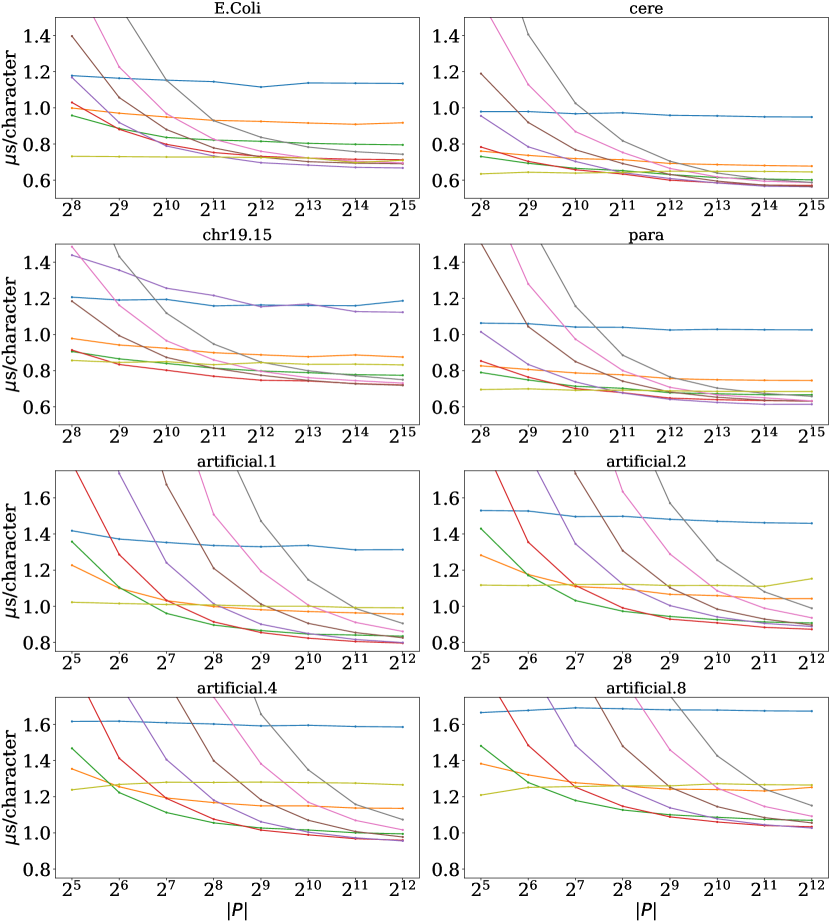
Figure 9: Time for answering ${{\textrm{{count}}}}{(P)}$, cf. Fig. 7

Table 4: Comparison of $\mathsf{RLFM}^{(0)}$ and $\mathsf{RLFM}^{(1)}$ on the real-world datasets described in Sect. 5. See Table 3 for a description of the columns.

input text			$\mathsf{RLFM}^{(0)}$		$\mathsf{RLFM}^{(1)}$
name	space [MiB]	$\sigma$	${r}^{(0)}$ [M]	space [MiB]	$\lambda$	space [MiB]	${\sigma}^{(1)}$	${r}^{(1)}$ [M]	$\lg|P|$
cere	439.9	6	11.6	26.8	1	26.5	6	11.6	-
					2	20.4	26	8.3	-
					3	18.4	95	6.7	12
					4	17.3	271	5.8	11
					5	16.7	602	5.3	11
					6	15.1	1081	5.1	12
					7	14.9	1790	5.0	13
					8	14.9	2810	4.9	13
chr19.15	845.8	6	32.3	70.8	1	69.7	6	32.3	-
					2	54.9	22	23.5	-
					3	50.8	58	19.0	10
					4	47.1	140	16.5	9
					5	44.9	305	15.1	-
					6	40.3	620	14.3	11
					7	39.7	1174	13.8	12
					8	39.4	2086	13.6	13
E.Coli	107.5	16	15.0	26.2	1	25.4	16	15.0	-
					2	20.4	123	10.7	-
					3	19.3	399	8.5	-
					4	17.8	809	7.3	13
					5	17.2	1272	6.7	12
					6	15.3	1764	6.3	13
					7	15.1	2356	6.2	13
					8	15.1	3251	6.1	-
para	409.4	6	15.6	34.4	1	34.0	6	15.6	-
					2	26.5	26	11.3	-
					3	24.5	96	9.1	12
					4	22.6	296	7.9	11
					5	20.0	774	7.2	11
					6	19.6	1620	6.9	12
					7	19.4	2701	6.7	13
					8	19.3	4013	6.7	14

Table 5: Comparison of $\mathsf{RLFM}^{(0)}$ and $\mathsf{RLFM}^{(1)}$ on the datasets of random generated DNA sequences. See Table 3 for a description of the columns.

input text			$\mathsf{RLFM}^{(0)}$		$\mathsf{RLFM}^{(1)}$
name	space [MiB]	$\sigma$	${r}^{(0)}$ [M]	space [MiB]	$\lambda$	space [MiB]	${\sigma}^{(1)}$	${r}^{(1)}$ [M]	$\lg|P|$
artificial.1	502.5	5	50.9	91.4	1	89.5	5	50.9	-
					2	84.9	17	39.0	8
					3	71.2	51	32.3	7
					4	69.2	131	28.7	8
					5	68.0	297	26.7	9
					6	67.4	611	25.8	10
					7	67.1	1164	25.3	11
					8	66.9	2058	25.1	11
artificial.2	500.0	5	87.5	141.8	1	138.5	5	87.5	-
					2	131.5	17	67.0	7
					3	111.8	51	55.5	7
					4	109.9	131	49.3	7
					5	108.5	297	45.9	9
					6	107.8	611	44.3	9
					7	107.4	1164	43.5	10
					8	107.2	2069	43.2	11
artificial.4	495.0	5	147.0	215.8	1	210.1	5	147.0	-
					2	198.7	17	111.4	6
					3	169.7	51	91.8	6
					4	168.4	131	81.1	7
					5	167.0	297	75.4	8
					6	166.0	611	72.6	9
					7	165.4	1164	71.3	10
					8	165.0	2077	70.7	11
artificial.8	485.0	5	237.4	300.2	1	290.9	5	237.4	-
					2	286.4	17	174.3	8
					3	239.6	51	141.3	7
					4	235.1	131	123.4	7
					5	231.0	297	113.9	8
					6	228.4	611	109.2	9
					7	226.6	1164	107.0	10
					8	225.5	2079	106.1	11

Table 6: Construction times on the real-world datasets. Times are in seconds ([s]).

dataset	FM-index	$\mathsf{RLFM}^{(0)}$	$\mathsf{RLFM}^{(1)}$
	time [s]	time [s]	$\lambda$	time [s]
cere	101.6	102.6	1	881.3
			2	471.4
			3	365.0
			4	299.4
			5	290.4
			6	277.4
			7	275.9
			8	276.6
chr19.15	207.7	208.9	1	2093.7
			2	1107.7
			3	807.3
			4	683.0
			5	633.2
			6	626.6
			7	609.6
			8	597.2
e.coli	24.5	25.0	1	187.1
			2	110.3
			3	87.1
			4	71.9
			5	66.7
			6	65.8
			7	66.3
			8	71.1
para	98.0	98.0	1	755.7
			2	410.5
			3	319.3
			4	267.4
			5	260.9
			6	251.5
			7	248.2
			8	252.2

Table 7: Construction times for the datasets artificial.$x$.

dataset	FM-index	$\mathsf{RLFM}^{(0)}$	$\mathsf{RLFM}^{(1)}$
	time [s]	time [s]	$\lambda$	time [s]
artificial.1	130.0	131.4	1	616.1
			2	339.4
			3	263.2
			4	227.4
			5	224.1
			6	230.7
			7	230.5
			8	233.7
artificial.2	129.2	132.9	1	578.2
			2	328.3
			3	254.5
			4	218.7
			5	213.2
			6	220.5
			7	220.3
			8	224.2
artificial.4	130.5	137.1	1	555.2
			2	555.2
			3	243.4
			4	213.6
			5	209.7
			6	218.1
			7	216.5
			8	222.8
artificial.8	132.4	144.4	1	530.6
			2	306.4
			3	241.0
			4	211.0
			5	207.1
			6	214.9
			7	215.5
			8	219.7

References

- Akagi et al. [2021] T. Akagi, D. Köppl, Y. Nakashima, S. Inenaga, H. Bannai, and M. Takeda. Grammar index by induced suffix sorting. CoRR, abs/2105.13744, 2021.
- Barbay et al. [2014] J. Barbay, F. Claude, T. Gagie, G. Navarro, and Y. Nekrich. Efficient fully-compressed sequence representations. Algorithmica, 69(1):232–268, 2014.
- Belazzougui and Navarro [2014] D. Belazzougui and G. Navarro. Alphabet-independent compressed text indexing. ACM Trans. Algorithms, 10(4):23:1–23:19, 2014.
- Belazzougui and Navarro [2015] D. Belazzougui and G. Navarro. Optimal lower and upper bounds for representing sequences. ACM Trans. Algorithms, 11(4):31:1–31:21, 2015.
- Burrows and Wheeler [1994] M. Burrows and D. J. Wheeler. A block sorting lossless data compression algorithm. Technical Report 124, Digital Equipment Corporation, Palo Alto, California, 1994.
- Charikar et al. [2005] M. Charikar, E. Lehman, D. Liu, R. Panigrahy, M. Prabhakaran, A. Sahai, and A. Shelat. The smallest grammar problem. IEEE Trans. Information Theory, 51(7):2554–2576, 2005.
- Christiansen et al. [2021] A. R. Christiansen, M. B. Ettienne, T. Kociumaka, G. Navarro, and N. Prezza. Optimal-time dictionary-compressed indexes. ACM Trans. Algorithms, 17(1):8:1–8:39, 2021.
- Clark [1996] D. R. Clark. Compact Pat Trees. PhD thesis, University of Waterloo, Canada, 1996.
- Claude and Navarro [2012] F. Claude and G. Navarro. Improved grammar-based compressed indexes. In Proc. SPIRE, volume 7608 of LNCS, pages 180–192, 2012.
- Claude et al. [2021] F. Claude, G. Navarro, and A. Pacheco. Grammar-compressed indexes with logarithmic search time. J. Comput. Syst. Sci., 118:53–74, 2021.
- Cormode and Muthukrishnan [2007] G. Cormode and S. Muthukrishnan. The string edit distance matching problem with moves. ACM Trans. Algorithms, 3(1):2:1–2:19, 2007.
- Díaz-Domínguez and Navarro [2020] D. Díaz-Domínguez and G. Navarro. A grammar compressor for collections of reads with applications to the construction of the BWT. CoRR, abs/2011.07999, 2020.
- Díaz-Domínguez and Navarro [2021] D. Díaz-Domínguez and G. Navarro. A grammar compressor for collections of reads with applications to the construction of the BWT. In Proc. DCC, pages 83–92, 2021.
- Díaz-Domínguez et al. [2021] D. Díaz-Domínguez, G. Navarro, and A. Pacheco. An LMS-based grammar self-index with local consistency properties. In Proc. SPIRE, 2021. To appear.
- Ferragina and Manzini [2000] P. Ferragina and G. Manzini. Opportunistic data structures with applications. In Proc. FOCS, pages 390–398, 2000.
- Ferragina et al. [2009] P. Ferragina, F. Luccio, G. Manzini, and S. Muthukrishnan. Compressing and indexing labeled trees, with applications. J. ACM, 57(1):4:1–4:33, 2009.
- Fischer et al. [2020] J. Fischer, T. I, and D. Köppl. Deterministic sparse suffix sorting in the restore model. ACM Trans. Algorithms, 16(4):50:1–50:53, 2020.
- Gagie et al. [2018] T. Gagie, G. Navarro, and N. Prezza. Optimal-time text indexing in BWT-runs bounded space. In Proc. SODA, pages 1459–1477, 2018.
- Gagie et al. [2019] T. Gagie, T. I, G. Manzini, G. Navarro, H. Sakamoto, and Y. Takabatake. Rpair: Rescaling RePair with Rsync. CoRR, abs/1906.00809, 2019.
- Ganczorz et al. [2018] M. Ganczorz, P. Gawrychowski, A. Jez, and T. Kociumaka. Edit distance with block operations. In Proc. ESA, volume 112 of LIPIcs, pages 33:1–33:14, 2018.
- Gog et al. [2014] S. Gog, T. Beller, A. Moffat, and M. Petri. From theory to practice: Plug and play with succinct data structures. In Proc. SEA, volume 8504 of LNCS, pages 326–337, 2014.
- Grossi et al. [2003] R. Grossi, A. Gupta, and J. S. Vitter. High-order entropy-compressed text indexes. In Proc. SODA, pages 841–850, 2003.
- Jacobson [1989] G. Jacobson. Space-efficient static trees and graphs. In Proc. FOCS, pages 549–554, 1989.
- Kärkkäinen et al. [2012] J. Kärkkäinen, P. Mikkola, and D. Kempa. Grammar precompression speeds up Burrows–Wheeler compression. In Proc. SPIRE, volume 7608 of LNCS, pages 330–335, 2012.
- Kempa and Kociumaka [2019] D. Kempa and T. Kociumaka. String synchronizing sets: sublinear-time BWT construction and optimal LCE data structure. In Proc. STOC, pages 756–767, 2019.
- Kempa and Prezza [2018] D. Kempa and N. Prezza. At the roots of dictionary compression: string attractors. In Proc. STOC, pages 827–840, 2018.
- Kieffer and Yang [2000] J. C. Kieffer and E. Yang. Grammar-based codes: A new class of universal lossless source codes. IEEE Trans. Information Theory, 46(3):737–754, 2000.
- Larsson and Moffat [1999] N. J. Larsson and A. Moffat. Offline dictionary-based compression. In Proc. DCC, pages 296–305, 1999.
- Mäkinen and Navarro [2005] V. Mäkinen and G. Navarro. Succinct suffix arrays based on run-length encoding. Nord. J. Comput., 12(1):40–66, 2005.
- Manber and Myers [1993] U. Manber and E. W. Myers. Suffix arrays: A new method for on-line string searches. SIAM J. Comput., 22(5):935–948, 1993.
- Mantaci et al. [2007] S. Mantaci, A. Restivo, G. Rosone, and M. Sciortino. An extension of the Burrows–Wheeler transform. Theor. Comput. Sci., 387(3):298–312, 2007.
- Manzini [2016] G. Manzini. XBWT tricks. In Proc. SPIRE, volume 9954 of LNCS, pages 80–92, 2016.
- Mehlhorn et al. [1997] K. Mehlhorn, R. Sundar, and C. Uhrig. Maintaining dynamic sequences under equality tests in polylogarithmic time. Algorithmica, 17(2):183–198, 1997.
- Nevill-Manning and Witten [1997] C. G. Nevill-Manning and I. H. Witten. Linear-time, incremental hierarchy inference for compression. In Proc. DCC, pages 3–11, 1997.
- Nong et al. [2011] G. Nong, S. Zhang, and W. H. Chan. Two efficient algorithms for linear time suffix array construction. IEEE Trans. Computers, 60(10):1471–1484, 2011.
- Nunes et al. [2018] D. S. N. Nunes, F. A. da Louza, S. Gog, M. Ayala-Rincón, and G. Navarro. A grammar compression algorithm based on induced suffix sorting. In Proc. DCC, pages 42–51, 2018.
{forest} for tree=draw,l sep+=1.4em [ [,edge label=node[lab] [,edge label=node[lab]a [,edge label=node[lab]a [,edge label=node[lab]c [A,edge label=node[lab]$]]] [,edge label=node[lab]b [B,edge label=node[lab]$]] [,edge label=node[lab]c [C,edge label=node[lab]$]] ] [,edge label=node[lab]b [D,edge label=node[lab]$] [,edge label=node[lab]c [E,edge label=node[lab]$]]]] ] F L symbol 0 a 0 b a 0 a a a 0 b a 1 c a 1 c aa b 0 $ b D b 1 c b 1 $ ba B c 1 $ ca C c 1 $ caa A c 1 $ cb E