Bell numbers in Matsunaga’s and Arima’s Genjikō combinatorics:
Modern perspectives and local limit theorems

Abstract.

We examine and clarify in detail the contributions of Yoshisuke Matsunaga (1694?–1744) to the computation of Bell numbers in the eighteenth century (in the Edo period), providing modern perspectives to some unknown materials that are by far the earliest in the history of Bell numbers. Later clarification and developments by Yoriyuki Arima (1714–1783), and several new results such as the asymptotic distributions (notably the corresponding local limit theorems) of a few closely related sequences are also given.

1. Introduction

1.1. Bell numbers

The Bell numbers $B_{n}$, counting the total number of ways to partition a set of $n$ labeled elements, are so named by Becker and Riordan [3]. While it is known that their first appearance can be traced back to the Edo period in Japan (see [11, 20, 21]), the history of these numbers is “a tricky business” [31, p. 105], and “the earliest occurrence in print of these numbers has never been traced” [32]; Rota added in [32]: “as expected, the numbers have been attributed to Euler, but an explicit reference has not been given”, obscuring further the early history of Bell numbers. Furthermore, in the words of Bell [4]: the $B_{n}$ “have been frequently investigated; their simpler properties have been rediscovered many times”. The recurrent rediscoveries, as well as the wide occurrence in diverse areas, in the last three centuries certainly testify the importance and usefulness of Bell numbers. See [25] for an instance of a typical rediscovery, and the OEIS webpage of Bell numbers OEIS A000110 for the diverse contexts where they appear. In particular, Bell numbers rank the 26th (among a total of 347,900+ sequences as of September 21, 2021) according to the number of referenced sequences in the OEIS database.

Bell numbers can be characterized and computed in many ways; indeed a few dozens of different expressions for characterizing $B_{n}$ are available on the OEIS webpage [29, A000110]. Among these, one of the most commonly used that is also by far the earliest one, often attributed to Yoshisuke Matsunaga’s unpublished work in the eighteenth century (see, e.g., [20, p. 504] or [23, Theorem 1.12]), is the recurrence

(1) $$B_{n} =\sum_{0\leqslant k<n}\binom{n-1}{k}B_{n-1-k},$$

for $n\geqslant 1$ with $B_{0}=1$. A more precise reference of this recurrence is Arima’s book “Shūki Sanpō” (Collections in Arithmetics [2]). More precisely, Knuth writes (his $\varpi_{n}$ is our $B_{n}$):

“Early in the 1700s, Takakazu Seki and his students began to investigate the number of set partitions $\varpi_{n}$ for arbitrary $n$, inspired by the known result that $\varpi_{5}=52$. Yoshisuke Matsunaga found formulas for the number of set partitions when there are $k_{j}$ subsets of size $n_{j}$ for $1\leqslant j\leqslant t$, with $k_{1}n_{1}+\cdots+k_{t}n_{t}=n$ (see the answer to exercise 1.2.5–21). He also discovered the basic recurrence relation 7.2.1.5–(14), namely

$$\varpi_{n+1}=\binom{n}{0}\varpi_{n}+\binom{n}{1}\varpi_{n-1}+\binom{n}{2}\varpi_{n-2}+\cdots+\binom{n}{n}\varpi_{0},$$

by which the values of $\varpi_{n}$ can readily be computed.

Matsunaga’s discoveries remained unpublished until Yoriyuki Arima’s book Shūki Sanpō came out in 1769. Problem $56$ of that book asked the reader to solve the equation “$\varpi_{n}=678570$” for $n$; and Arima’s answer, worked out in detail (with credit duly given to Matsunaga), was $n=11$.”

1.2. Yoshisuke Matsunaga

However, as will be clarified in this paper, Yoshisuke Matsunaga (松永良弼) indeed used a very different procedure (see Theorem 1 below) in his 1726 book [24] to compute $B_{n}$, which was later expounded in detail and modified by Yoriyuki Arima (有馬頼徸) in his 1763 book [1] (not his 1769 Shūki Sanpō [2]), eventually led to the recurrence (1). It would then be natural to call the sequence $\binom{n-1}{k}B_{n-1-k}$ the Arima numbers; see Section 5 for their distributional aspect. Informative materials on the life and mathematical works of Matsunaga can be found in the two books (in Japanese) by Fujiwara [10] and by Hirayama [14], respectively.

Briefly, Yoshisuke Matsunaga (born in 1694? and died in 1744) was a mathematician in the Edo period (江戸時代). His original surname was Terauchi (寺内), and also known under a few different names such as Heihachiro (平八郎), Gonpei (權平), and Yasuemon (安右衛門); other names used include Higashioka (東岡), Tangenshi (探玄子), etc. Matsunaga served first in the Arima family in Kurume Domain (久留米藩); he also learned Wasan (和算, Japanese Mathematics) from Murahide Araki (荒木村英) who was a disciple of Takakazu Seki (関孝和), the founder of modern Wasan. He then came to Iwakidaira Domain (磐城平藩) and was employed by Masaki Naito (内藤政樹) in 1732. There, he worked with Yoshihiro Kurushima (久留島義太), and his research was believed to be influenced by the theory of Kenko Takebe (建部賢弘) and other Seki disciples. He developed and largely improved Seki’s Mathematics. One of his representative achievements is the calculation of $\pi$ (circumference-diameter ratio of a circle) to 51 digits (of which the first 49 are correct; see [10, p. 457]). He is also known to compute the series expansions of trigonometric functions such as sine, cosine, arc-sine, etc. For more information, see [10, 14]. See also this webpage for more information on Japanese Mathematics in the Edo Period.

1.3. The Genjikō game.

The set-partition combinatorics developed by the Wasanists in the Edo period was largely motivated by the parlor game called Genjikō (源氏香, literally Genji incense, where Genji refers to the famous novel Genji Monogatari (源氏物語), or The Tale of Genji by Murasaki-Shikibu, 紫式部), as already mentioned in the combinatorial literature; see [11, 20, 23] and the webpage [21].

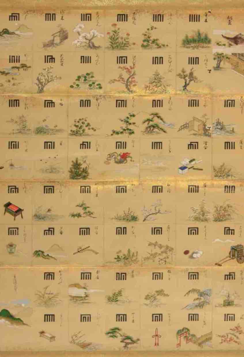
Figure 1. A Genjikōnozu-painting by Mitsuoki Tosa (土佐光起, 1617–1691) collected at Wadeda University Library (image courtesy of Waseda University Library).

According to the preface of Arima’s book [1] (see also [12, p. 332]):

While Takakazu Seki initiated the study of Genjikō combinatorics (or the techniques of separate-and-link), it was Matsunaga and his contemporary Kurushima who probed its origin and developed fundamentally the techniques.

The game is part of the Japanese Kōdō (香道, or the Way of Fragrance, the same character “kō” 香, also means fragrance) to appreciate the fragrances of the incense. It was established in the late Muromachi period (室町時代) in the sixteenth century and became popular in the upper class during the Edo period. It consists of the following steps:

1. Five different types of incense sticks are cut into five pieces each;

2. Five of these 25 pieces are chosen to be smoldered;

3. Guests smell each incense and try to discern (or “listen to” in a silent ambience and calm mood) which among the five incenses chosen are the same and which are different;

4. On the answer sheets, guests write their names and the conjectured composition of the incenses already smoldered as Genjikōnozu (源氏香の図 or Genjimon, 源氏紋, meaning the patterns of Genjikō). The Genjikōnozu is composed of five vertical bars for the five incenses in right-to-left order; then link the vertical bars with a horizontal line on top if the corresponding incenses are thought to be the same.). See for example Figure 1 for one of the earliest paintings about Genjikōnozu found so far.

5. The game has no winners or losers; if the answer is correct, the five-stroke Kanji character 玉 (meaning literally “jade” and figuratively something precious or beautiful) is written on the answer sheet.

In addition to the Genjikōnozus used to represent the patterns of incenses, a chapter name from The Tale of Genji is also associated with each of the 52 configurations of the five incenses, not only for easier reference and use but sometimes also for a reading of that chapter; see Figure 2. Partly due to such an unusual association and their unusual aesthetic, cryptic features, the Genjikōnozus continue to be used in the design of diverse modern applications such as patterns on kimono, wrapping papers, folding screens, badges, etc.

Kiritsubo

桐壺

Hahakigi

帚木

Utsusemi

空蝉

Yugao

夕顔

Wakamurasaki

若紫

Suetsumuhana

末摘花

Momijinoga

紅葉賀

Hananoen

花宴

Aoi

葵

Sakaki

賢木

Hanachirusato

花散里

Suma

須磨

Akashi

明石

Miotsukushi

澪標

Yomogiu

蓬生

Sekiya

関屋

Eawase

絵合

Matsukaze

松風

Usugumo

薄雲

Asagao

朝顔

Otome

少女

Tamakazura

玉鬘

Hatsune

初音

Kochou

胡蝶

Hotaru

蛍

Tokonatsu

常夏

Kagaribi

篝火

Nowaki

野分

Miyuki

行幸

Fujibakama

藤袴

Makibashira

真木柱

Umegae

梅枝

Fujinouraba

藤裏葉

Wakana I

若菜上

Wakana II

若菜下

Kashiwagi

柏木

Yokobue

横笛

Suzumushi

鈴虫

Yugiri

夕霧

Minori

御法

Maboroshi

幻

Nioumiya

匂宮

Koubai

紅梅

Takekawa

竹河

Hashihime

橋姫

Shiigamoto

椎本

Agemaki

総角

Sawarabi

早蕨

Yadorigi

宿木

Azumaya

東屋

Ukifune

浮舟

Kagerou

蜻蛉

Tenarai

手習

Yumenoukihashi

夢浮橋

Figure 2. The 52 Genjikō patterns arranged in the chapter order (top-down and left-to-right) of the novel Genji Monogatari (54 chapters).

2. Matsunaga’s procedure to compute $B_{n}$

2.1. Matsunaga’s 1726 book [24]

Matsunaga wrote voluminously on a broad range of topics in Wasan (more than 50 titles listed in Hirayama’s book [14]), but none of these was printed and published during his life time due partly to the tradition at that time; it is therefore common to find different hand-written versions of the same book.

Among his books the one dated 1726 and entitled Danren Sōjutsu (断連総術, literally General techniques of separate-and-link) [24] (with a total of 11 double-pages) is indeed completely devoted to the calculation of Bell numbers, aiming specially to enumerate all possible ways to connect and to separate a given number of incenses in the Genjikō game.

Our first aim in this paper is to provide more details contained in this book [24], and to highlight his procedure to compute Bell numbers, which is nevertheless not the equation (1) as most authors believed and referenced. This book, as well as a few others mentioned in this paper, is freely available at the webpage of National Institute of Japanese Literature (NIJL). Since all these ancient books do not have page numbers (and the page numbers differ in different versions of the same book), all page numbers referenced in this paper are indeed the (double) page order of the corresponding digital file at the NIJL database. We will provide the corresponding URLs whenever possible.

Matsunaga’s procedure was later examined and improved in great detail in Arima’s 1763 book [1] on “Variational techniques of separate-and-link” (断連変局法, about 55 double-pages), and there we find the occurrence of the recurrence (1); see Section 5 for more details.

2.2. Matsunaga numbers

Let $s_{n,k}$ denote (signed) Stirling numbers of the first kind (see A008275 and A048994), and $\genfrac{[}{]}{0.0pt}{}{n}{k}=(-1)^{n-k}s_{n,k}$ the unsigned version (see A132393). Denote by $[z^{n}]f(z)$ the coefficient of $z^{n}$ in the Taylor expansion of $f(z)$.

Theorem 1 (Matsunaga, 1726 [24]).

For $n\geqslant 1$

(2) $$B_{n}=1+\frac{1}{n!}\sum_{1\leqslant k\leqslant n}M_{n,k}n^{k},$$

where the Matsunaga numbers $M_{n,k}$ are defined recursively by

(3) $$M_{n,k}=nM_{n-1,k}+\beta_{n}s_{n,k}$$

for $1\leqslant k\leqslant n$ with the boundary conditions $M_{n,k}=0$ for $n\leqslant 1$, $k\leqslant 0$ and $k>n$. Here $\beta_{n}:=n![z^{n}]e^{e^{z}-1-z}$ counts the number of set partitions of $n$ elements without singletons.

Proof.

A direct iteration of $\eqref{E:bnk}$ gives

(4) $$M_{n,k}=n!\sum_{k\leqslant j\leqslant n}\frac{\beta_{j}}{j!}\,s_{j,k}.$$

Then, by the defining relation of Stirling numbers of the first kind,

$$\sum_{1\leqslant k\leqslant m}s_{m,k}z^{k}=z(z-1)\cdots(z-m+1),$$

we have

$$\begin{split}1+\frac{1}{n!}\sum_{1\leqslant k\leqslant n}M_{n,k}n^{k}&=1+\sum_{1\leqslant k\leqslant n}n^{k}\sum_{k\leqslant j\leqslant n}\frac{\beta_{j}}{j!}\,s_{j,k}\\ &=1+\sum_{1\leqslant j\leqslant n}\frac{\beta_{j}}{j!}\sum_{1\leqslant k\leqslant j}s_{j,k}n^{k}\\ &=1+\sum_{1\leqslant j\leqslant n}\frac{\beta_{j}}{j!}\,n(n-1)\cdots(n-j+1)\\ &=n!\sum_{0\leqslant j\leqslant n}\frac{\beta_{j}}{j!}\cdot\frac{1}{(n-j)!}\\ &=n![z^{n}]e^{e^{z}-1-z}\cdot e^{z}=B_{n},\end{split}$$

with $\beta_{0}=1$. Combinatorially, the last relation is equivalent to splitting set partitions into those with blocks of size $1$ and those without. ∎

Note that $B_{n}=\beta_{n+1}+\beta_{n}$, which, by a direct iteration, gives

(5) $$\beta_{n}=\sum_{0\leqslant j<n}(-1)^{n-1-j}B_{j}+(-1)^{n}\qquad(n\geqslant 0).$$

The first few terms of $\beta_{n}$ are given by (see OEIS A000296)

$$\{\beta_{n}\}_{n\geqslant 1}=\{0,1,1,4,11,41,162,715,3425,17722,98253,580317,\dots\},$$

and Table 1 gives the first few rows of $M_{n,k}$ for $n=1,\dots,7$; these numbers already appeared in [24] and [1].

$n\backslash k$	$1$	$2$	$3$	$4$	$5$	$6$	$7$
$1$	$0$
$2$	$-1$	$1$
$3$	$-1$	$0$	$1$
$4$	$-28$	$44$	$-20$	$4$
$5$	$124$	$-330$	$285$	$-90$	$11$
$6$	$-4176$	$9254$	$-7515$	$2945$	$-549$	$41$
$7$	$87408$	$-220990$	$210483$	$-98455$	$24507$	$-3115$	$162$

Table 1. The values of $M_{n,k}$ for $n=1,\dots,7$ and $1\leqslant k\leqslant n$. Each row sum is zero.

2.3. The “non-conventional” procedure to compute $B_{n}$

Matsunaga’s extraordinary procedure to compute $B_{n}$ is then as follows (extraordinary in the sense that we have not found it in the combinatorial literature).

• Tabulate first $s_{n,k}$ [24, pp. 2–3];

• Compute $\beta_{n}$ by a direct exhaustive combinatorial enumeration [24, pp. 3–6] and [24, pp. 8–10];

• Tabulate $M_{n,k}$ by using the recurrence (3) [24, p. 7];

• Evaluate the polynomial (in $n$) $\sum_{k}M_{n,k}n^{k}$ by Horner’s rule [24, p. 7]:

  $$\sum_{1\leqslant k\leqslant n}M_{n,k}n^{k}=n\bigl{(}{M_{n,1}+n\bigl{(}{M_{n,2}+\cdots+n(M_{n,n-1}+M_{n,n}n)}\bigr{)}}\bigr{)};$$

• Then dividing the above sum by $n!$ and adding $1$ yields $B_{n}$, where the values $B_{2},\dots,B_{8}$ are given [24, pp. 10–11].

Note that the origin of Horner’s rule can be traced back to Chinese and Persian Mathematics in the thirteenth century.

In particular,

(6) $$\begin{split}B_{2}&=1+\frac{1}{2!}\cdot 2(\underline{-1}+\underline{1}\cdot 2)=1+\frac{2\cdot 1}{2}=2\\ B_{3}&=1+\frac{1}{3!}\cdot 3(\underline{-1}+3(\underline{0}+\underline{1}\cdot 3))=1+\frac{3\cdot 8}{6}=5\\ B_{4}&=1+\frac{1}{4!}\cdot 4(\underline{-28}+4(\underline{44}+4(\underline{-20}+\underline{4}\cdot 4)))=1+\frac{4\cdot 84}{24}=15\\ B_{5}&=1+\frac{1}{5!}\cdot 5(\underline{124}+5(\underline{-330}+5(\underline{285}+5(\underline{-90}+\underline{11}\cdot 5))))=1+\frac{5\cdot 1224}{120}=52,\end{split}$$

where the Matsunaga numbers (see Table 1) are underlined.

$n\backslash k$	$1$	$2$	$3$	$4$	$5$	$6$	$B_{n}$
$2$	$-2$	$4$					$2$
$3$	$-3$	$0$	$27$				$5$
$4$	$-112$	$704$	$-1280$	$1024$			$15$
$5$	$620$	$-8250$	$35625$	$-56250$	$34375$		$52$
$6$	$-25056$	$333144$	$-1623240$	$3816720$	$-4269024$	$1912896$	$203$

Table 2. The values of $M_{n,k}n^{k}$ for $n=2,\dots,6$ and $1\leqslant k\leqslant n$; they are mostly much larger in modulus than $B_{n}$

2.4. First appearance of $s_{n,k}$

On the other hand, a careful reader will notice the time difference between Matsunaga’s use of $s_{n,k}$ in his 1726 book and Stirling’s introduction of these numbers in 1730. Indeed, Stirling numbers of the first kind already appeared earlier in Seki’s posthumous book “Katsuyō Sanpō” (括要算法, Compendium of Arithmetics [33]) published in 1712, and thus were not new to the followers of the Seki School. In particular, the recurrence formula

$$s_{n,k}=s_{n-1,k-1}-(n-1)s_{n-1,k}$$

is given in Seki’s book (see Figure 3). On the other hand, it is also known that Stirling numbers of the first kind can be traced earlier back to Harriot’s manuscripts near the beginning of the 17th century; see [19].

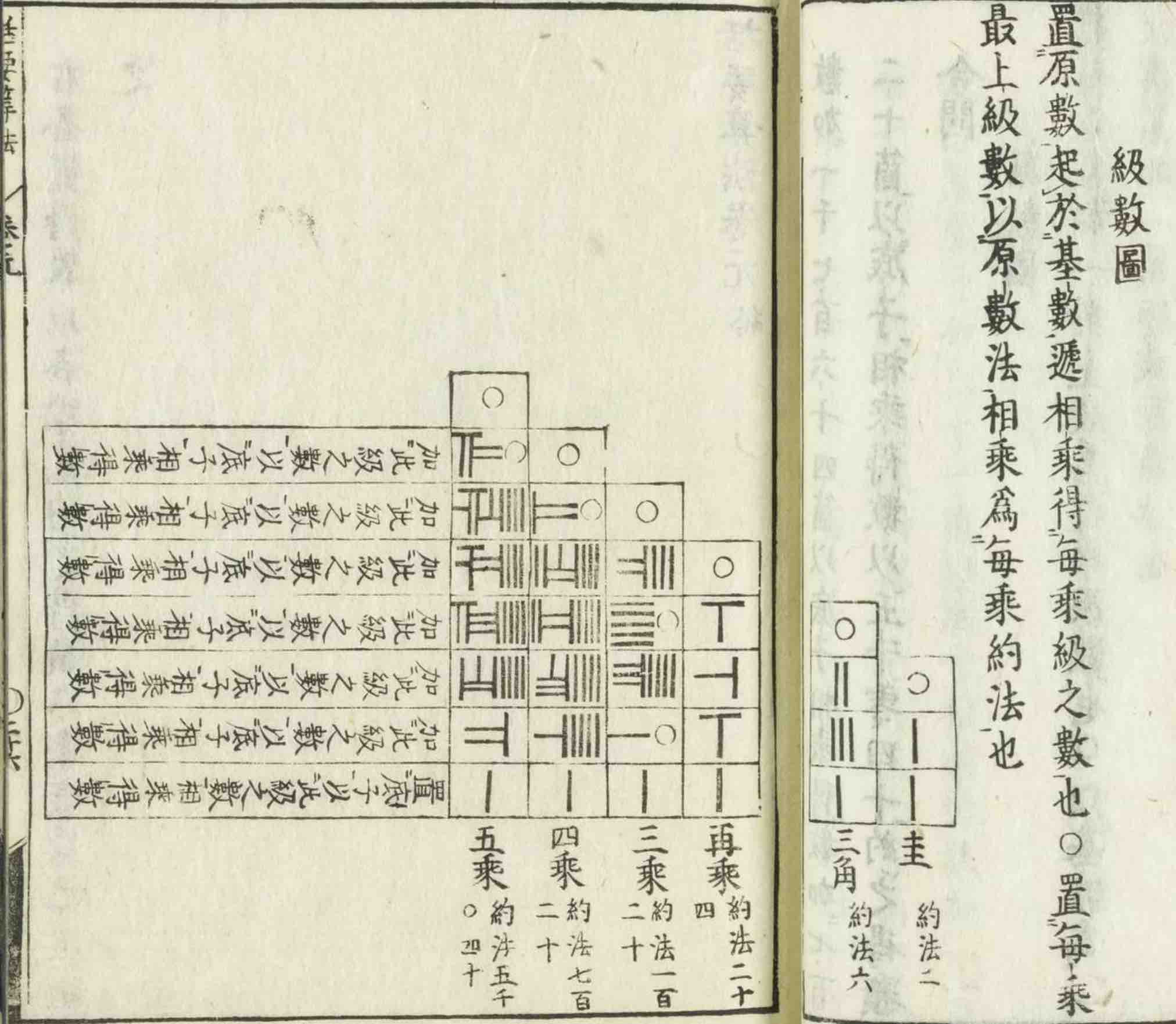
$0$
$720$	$0$
$1764$	$120$	$0$
$1624$	$274$	$24$	$0$
$735$	$225$	$50$	$6$	$0$
$175$	$85$	$35$	$11$	$2$	$0$
$21$	$15$	$10$	$6$	$3$	$1$
$1$	$1$	$1$	$1$	$1$	$1$
$5040$	$720$	$120$	$\ 24$	$\ \ 6$	$\ \ 2$

Figure 3. Left: page 33 (image from the digital collections of The National Diet Library of Japan) of Seki’s book [33] where Stirling numbers of the first kind appear; the recurrence is described on the leftmost margin. Right: the unsigned Stirling numbers as displayed in Seki’s table written in their modern forms.

Due to their diverse use in different contexts, the Stirling numbers $s_{n,k}$ (A008275) have a large number of variants; common ones collected in the OEIS include the following ones:

• additional zeroth column: (A048994),

• unsigned version: $|s_{n,k}|$ (A130534),

• row-reversed: $s_{n,n+1-k}$ (A008276),

• multiples: $(n+1)\genfrac{[}{]}{0.0pt}{}{n}{k}$ (A180013), which enumerates the number of fixed points in permutations of $n$ elements with $k$ cycles,

• unsigned, row-reversed: $|s_{n,n+1-k}|$ (A094638),

• unsigned, additional zeroth column: (A132393).

2.5. Inefficiency of the procedure

While the proof of (2) is straightforward, the fact that the circuitous expression (2) represents by far the earliest way to compute $B_{n}$ comes as a surprise. Even more surprising is that such a procedure is indeed extremely inefficient from a computational viewpoint, since it involves computing large numbers with alternating signs (see Table 2 and (6)), resulting in violent cancellations as $n$ increases. In fact, since Stirling numbers of the first kind may grow as large as $n!/\sqrt{\log n}$ in absolute value near their peaks (see [16] or (20) below) and $n^{k}$ is also factorially large for linear $k$, the cancellations occur indeed at a factorial scale. This might also explain why Matsunaga computed $B_{n}$ only for $n\leqslant 8$ in the end of [24]. On the other hand, from (2), we see that

$$\sum_{1\leqslant k\leqslant n}M_{n,k}n^{k}=(B_{n}-1)n!.$$

Thus if no better numerical procedure is introduced to handle the calculation of the normalized sum $\sum_{1\leqslant k\leqslant n}M_{n,k}n^{k}/n!$, then intermediate steps will involve numbers as large as $B_{n}\times n!$, which grows like

$$\log\Bigl{(}{\sum_{1\leqslant k\leqslant n}M_{n,k}n^{k}}\Bigr{)}\sim\log B_{n}n!\sim 2n\log n-n\log\log n-n,$$

(see (24) below), which is close to $2\log n!$.

So one naturally wonders whether Matsunaga was led to this procedure by roughly following backward the same reasoning as that given in the proof of (2). The inefficiency was noticed in later works such as in Arima’s book [1], and there the more efficient recurrence (1) is given.

3. Distribution of Matsunaga numbers

The above numerical viewpoint for Matsunaga’s procedure naturally motivates the question: how does the numbers $|M_{n,k}|$ distribute for large $n$ and varying $k$? This question also has its own interest per se in view of the historical importance of this sequence.

3.1. Identities

We derive first a more practical expression for $|M_{n,k}|$ because the sum expression (4) becomes less convenient with the absolute value sign.

Lemma 1.

For $1\leqslant k\leqslant n$, $n\geqslant 1$ and $(n,k)\neq(3,1)$,

(7) $$|M_{n,k}|=n!\sum_{k\leqslant j\leqslant n}\frac{(-1)^{n-j}\beta_{j}}{j!}\,|s_{j,k}|.$$

Proof.

First, by the alternating-sign relation $|s_{j,k}|=(-1)^{j+k}s_{j,k}$,

(8) $$\frac{|M_{n,k}|}{n!}=\left|\sum_{k\leqslant j\leqslant n}\frac{\beta_{j}}{j!}\,s_{j,k}\right|=\pm\sum_{k\leqslant j\leqslant n}\frac{(-1)^{n-j}\beta_{j}}{j!}\,|s_{j,k}|.$$

For $0\leqslant n\leqslant 3$ and $1\leqslant k\leqslant n$, it is easily checked that the equality holds with a plus sign in front of the second sum in (8) except for the pair $(n,k)=(3,1)$ where the two sides of (8) differ by a minus sign. We now show that the sequence $\{\beta_{n}|s_{n,k}|/n!\}_{n}$ is nondecreasing for $n\geqslant\max\{k,4\}$ and fixed $k\geqslant 1$, implying that (8) holds with the plus sign and in turn that (7) is valid. Since

(9) $$|s_{n,k}|=|s_{n-1,k-1}|+(n-1)|s_{n-1,k}|,$$

we have the trivial inequality $|s_{n+1,k}|\geqslant n|s_{n,k}|$; thus it suffices to prove that

(10) $$\frac{\beta_{n+1}}{n+1}\geqslant\frac{\beta_{n}}{n},\qquad(n\geqslant 3).$$

For that purpose, we use the recurrence

$$\beta_{n+1}=\sum_{0\leqslant j\leqslant n-1}\binom{n}{j}\beta_{j}\qquad(n\geqslant 1),$$

with the initial conditions $\beta_{0}=1$ and $\beta_{1}=0$, which is obtained by taking derivative of the exponential generating function (EGF) $e^{e^{z}-1-z}$ of $\beta_{n}$ and by equating the coefficients. Then (10) follows from the inequality

$$\binom{n}{j}=\frac{n}{n-j}\binom{n-1}{j}\geqslant\frac{n+1}{n}\binom{n-1}{j}\qquad(1\leqslant j<n).\qed$$

Define $P_{n}(v):=\sum_{1\leqslant k\leqslant n}|M_{n,k}|v^{k}$.

Proposition 1.

For $n\geqslant 4$,

(11) $$\frac{P_{n}(v)}{n!}=\sum_{0\leqslant j\leqslant n-2}\binom{v+n-j-1}{n-j}(-1)^{j}\beta_{n-j}\qquad(n\geqslant 4).$$

Proof.

This follows from (7) and the generating polynomial

$$\sum_{1\leqslant k\leqslant n}|s_{n,k}|z^{k}=z(z+1)\cdots(z+n-1).\qed$$

Corollary 1.

For $n\geqslant 4$

$$\frac{P_{n}(1)}{n!}=\sum_{0\leqslant j\leqslant n-2}(-1)^{j}\beta_{n-j}=\sum_{0\leqslant j<n}(-1)^{j}(j+1)B_{n-1-j}+(-1)^{n}n.$$

Proof.

Substitute $v=1$ in (11) and then use (5). ∎

By the ordinary generating function of the Bell numbers, we also have the relation

$$\frac{P_{n}(1)}{n!}=[z^{n}]\frac{z}{(1+z)^{2}}\sum_{k\geqslant 1}\prod_{1\leqslant j\leqslant k}\frac{z}{1-jz}\qquad(n\geqslant 4).$$

Note that $P_{n}(1)=\sum_{1\leqslant j\leqslant n}|M_{n,j}|\sim\beta_{n}n!$ while $\sum_{1\leqslant j\leqslant n}M_{n,j}=0$.

3.2. Asymptotics

In this section, we turn to the asymptotics and show that $|M_{n,k}|$ is very close to $\beta_{n}|s_{n,k}|$ for large $n$, so the distributional properties of $|M_{n,k}|$ will mostly follow from those of $|s_{n,k}|$.

Proposition 2.

Uniformly for $1\leqslant k\leqslant n$

(12) $$M_{n,k}=\beta_{n}s_{n,k}\bigl{(}{1+O\bigl{(}{n^{-1}\log n}\bigr{)}}\bigr{)}.$$

Thus only the term with $j=n$ in the sum expression (4) is dominant for large $n$; see Figure 4.

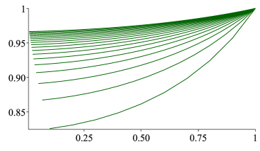
Figure 4. Uniformity of the ratios of $M_{n,k}$ to $\beta_{n}s_{n,k}$ for $1\leqslant k\leqslant n$ and $n=10,15,\dots,100$ (in bottom-up order). The approximation is seen to be good even for moderate values of $n$.

3.2.1. Asymptotics of $\beta_{n}$

Recall that $\beta_{n}:=n![z^{n}]e^{e^{z}-1-z}$ denotes the number of set partitions without singletons. Let $W(x)>0$ denote the (principal branch of) Lambert $W$-function, which satisfies the equation $We^{W}=x$ (and is positive for positive $x$). Asymptotically, for large $x$

$$W(x)=\log x-\log\log x+\frac{\log\log x}{\log x}+O\bigl{(}{(\log x)^{-2}(\log\log x)^{2}}\bigr{)};$$

see Corless et al.’s survey paper  [7] for more information on $W(x)$.

Lemma 2.

For large $n$ ($w:=W(n)$)

(13) $$\beta_{n}=\frac{e^{(w+w^{-1}-1)n-w-1}}{\sqrt{w+1}}\Bigl{(}{1-\frac{26w^{4}+67w^{3}+46w^{2}}{24n(w+1)^{3}}+O\bigl{(}{n^{-2}(\log n)^{2}}\bigr{)}}\Bigr{)}.$$

Proof.

This follows from applying the standard saddle-point method to Cauchy’s integral formula:

$$\beta_{n}=\frac{n!}{2\pi i}\oint_{|z|=r_{0}}z^{-n-1}e^{e^{z}-1-z}{\,\rm d}z,$$

where $r_{0}=r_{0}(n)>0$ solves the saddle-point equation

$$r_{0}(e^{r_{0}}-1)=n,$$

which satisfies asymptotically (by Lagrange inversion formula [9, A.6])

$$r_{0}=w+\sum_{j\geqslant 1}\eta_{j}n^{-j},\quad\text{with}\quad\eta_{j}=\frac{1}{j}[t^{j-1}]\Bigl{(}{\frac{wt(w+t)}{(w+t)e^{t}-w}}\Bigr{)}^{j}.$$

In particular,

$$r_{0}=w+\frac{w^{2}}{n(w+1)}-\frac{w^{3}(w^{2}-2)}{2n^{2}(w+1)^{3}}+O\bigl{(}{n^{-3}w^{3}}\bigr{)}.$$

See [8], [27], or [9] for similar details concerning Bell numbers or the saddle-point method. ∎

Corollary 2.

For large $n$ and $\ell=O(1)$

(14) $$\frac{\beta_{n-\ell}}{\beta_{n}}=\Bigl{(}{\frac{W(n)}{n}}\Bigr{)}^{\ell}\bigl{(}{1+O\bigl{(}{n^{-1}\ell^{2}\log n}\bigr{)}}\bigr{)}.$$

Proof.

By the saddle-point approximation (13) and the expansion

(15) $$W(n-t)=W(n)-\frac{W(n)t}{n(W(n)+1)}+O\bigl{(}{n^{-2}t^{2}}\bigr{)},$$

for $t=O(1)$, where the relation $W^{\prime}(x)=\frac{W(x)}{x(W(x)+1)}$ is used; see [7, Eqs. (3.2) and (3.3)]. ∎

3.2.2. Proof of Proposition 2

We are now ready to prove Proposition 2.

Proof.

From (4), we have

$$\frac{M_{n,k}}{\beta_{n}}=s_{n,k}\biggl{(}{1+O\biggl{(}{\sum_{1\leqslant j\leqslant n-k}\frac{n!}{(n-j)!}\cdot\frac{\beta_{n-j}}{\beta_{n}}\cdot\frac{|s_{n-j,k}|}{|s_{n,k}|}}\biggr{)}}\biggr{)}.$$

Now by the recurrence (9), we have the trivial inequalities

$$|s_{n,k}|\geqslant(n-1)|s_{n-1,k}|\geqslant(n-1)(n-2)|s_{n-2,k}|\geqslant\cdots\geqslant(n-1)\cdots(n-j)|s_{n-j,k}|,$$

which then give

$$\sum_{1\leqslant j\leqslant n-k}\frac{n!}{(n-j)!}\cdot\frac{\beta_{n-j}}{\beta_{n}}\cdot\frac{|s_{n-j,k}|}{|s_{n,k}|} \leqslant\sum_{1\leqslant j\leqslant n-k}\frac{\beta_{n-j}}{\beta_{n}}\cdot\frac{n}{n-j}$$

$$=O\Bigl{(}{\frac{\log n}{n}}\Bigr{)},$$

by the relation (14). This completes the proof of (12). ∎

Extending the same proof shows that (7) is itself an asymptotic expansion for large $n$ and each $k\in[1,n-1]$, namely,

$$\frac{|M_{n,k}|}{\beta_{n}|s_{n,k}|}=1+\sum_{1\leqslant j<J}(-1)^{j}\frac{n!}{(n-j)!}\cdot\frac{\beta_{n-j}}{\beta_{n}}\cdot\frac{|s_{n-j,k}|}{|s_{n,k}|}+O\bigl{(}{n^{-J}(\log n)^{J}}\bigr{)},$$

for any bounded $J\geqslant 1$ satisfying $J\leqslant n-k$.

3.3. Asymptotic distributions

With the closed-form (11) and the uniform approximation (12) available, all distributional properties of $|M_{n,k}|$ can be translated into those of $|s_{n,k}|$. For simplicity, we introduce the following notation and say that $\{a_{n,k}\}_{k}$ satisfies the local limit theorem (LLT):

$$\{a_{n,k}\}_{k}\,\simeq\,\mathrm{LLT}\bigl{(}{\mu_{n},\sigma^{2}_{n};\varepsilon_{n}}\bigr{)},$$

for large $n$ and positive sequence $a_{n,k}$ if the underlying sequence of random variables

$$\mathbb{P}(X_{n}=k):=\frac{a_{n,k}}{\sum_{j}a_{n,j}},$$

satisfies $\mathbb{E}(X_{n})\sim\mu_{n}$, $\mathbb{V}(X_{n})\sim\sigma^{2}_{n}$, and

$$\sup_{x\in\mathbb{R}}\sigma_{n}\Bigl{|}\mathbb{P}(X_{n}=\mu_{n}+x\sigma_{n})-\frac{e^{-\frac{1}{2}x^{2}}}{\sqrt{2\pi}}\Bigr{|}=O(\varepsilon_{n}),$$

with $\sigma_{n}\to\infty$ and $\varepsilon_{n}\to 0$. When the convergence rate is immaterial, we also write $\mathrm{LLT}(\mu_{n},\sigma_{n}^{2})=\mathrm{LLT}(\mu_{n},\sigma_{n}^{2};o(1))$. Similarly, the notations $\mathscr{N}(\mu_{n},\sigma_{n}^{2})$ and $\mathscr{N}(\mu_{n},\sigma_{n}^{2};\varepsilon_{n})$ denote the central limit theorem (CLT or weak convergence to standard normal law) with convergence rates $o(1)$ and $\varepsilon_{n}$, respectively.

Theorem 2.

(16) $$\{|M_{n,k}|\}_{k}\,\simeq\,\mathrm{LLT}\bigl{(}{\log n,\log n;(\log n)^{-\frac{1}{2}}}\bigr{)}.$$

See [15, 16, 30] for other properties of the Stirling cycle distribution.

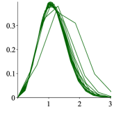
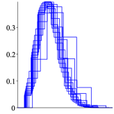
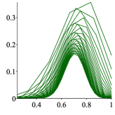
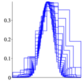
$\frac{|M_{n,x\log n}|}{\sum_{1\leqslant j\leqslant n}|M_{n,j}|}$	$\frac{|M_{n,\left\lfloor x\log n\right\rfloor}|}{\sum_{1\leqslant j\leqslant n}|M_{n,j}|}$	$\frac{|M_{n,xn}|n^{xn}}{\sum_{1\leqslant j\leqslant n}|M_{n,j}|n^{j}}$	$\frac{|M_{n,\left\lfloor xn\right\rfloor}|n^{\left\lfloor xn\right\rfloor}}{\sum_{1\leqslant j\leqslant n}|M_{n,j}|n^{j}}$
$n=5\ell,1\leqslant\ell\leqslant 12$		$6\leqslant n\leqslant 30$	$n=3\ell,2\leqslant\ell\leqslant 15$

Figure 5. Different graphical renderings of histograms of $|M_{n,k}|$ (the left two) and $|M_{n,k}|n^{k}$ (rightmost and middle-right). All plots, except for the third one, are scaled by the standard deviations.

Proof.

For the proof of Theorem 2, we begin with the calculations of the mean and the variance. For convenience, define

$$\mathbb{E}\bigl{(}{v^{X_{n}}}\bigr{)}:=\frac{P_{n}(v)}{P_{n}(1)}.$$

Then, by (11), we obtain, for $n\geqslant 4$

$$\mathbb{E}(X_{n})=\frac{\displaystyle\sum_{0\leqslant j\leqslant n-2}(-1)^{j}\beta_{n-j}H_{n-j}}{\displaystyle\sum_{0\leqslant j\leqslant n-2}(-1)^{j}\beta_{n-j}}=\frac{\beta_{n}H_{n}-\beta_{n-1}H_{n-1}+-\cdots}{\beta_{n}-\beta_{n-1}+-\cdots},$$

where $H_{n}^{[m]}:=\sum_{1\leqslant j\leqslant n}j^{-m}$ denotes the harmonic numbers and $H_{n}:=H_{n}^{[1]}$. Similarly, the variance is given by

$$\mathbb{V}(X_{n})=\frac{\displaystyle\sum_{0\leqslant j\leqslant n-2}(-1)^{j}\beta_{n-j}(H_{n-j}^{2}-H_{n-j}^{[2]})}{\displaystyle\sum_{0\leqslant j\leqslant n-2}(-1)^{j}\beta_{n-j}}-\mathbb{E}(X_{n})^{2}+\mathbb{E}(X_{n}),$$

for $n\geqslant 4$. Note that each of these sums is itself an asymptotic expansion in view of (14); more precisely, if a given sequence $\{\alpha_{n}\}$ satisfies $\alpha_{n-1}/\alpha_{n}\to c$, where $c>0$, then, by (14), we can group the terms in the following way

$$\frac{\displaystyle\sum_{0\leqslant j\leqslant n-2}(-1)^{j}\alpha_{n-j}\beta_{n-j}}{\displaystyle\sum_{0\leqslant j\leqslant n-2}(-1)^{j}\beta_{n-j}} =\alpha_{n}\biggl{(}1-\frac{\beta_{n-1}}{\beta_{n}}\Bigl{(}{1-\frac{\alpha_{n-1}}{\alpha_{n}}}\Bigr{)}$$

$$\qquad+\Bigl{(}{\frac{\beta_{n-1}}{\beta_{n}}}\Bigr{)}^{2}\Bigl{(}{1-\frac{\alpha_{n-1}}{\alpha_{n}}}\Bigr{)}-\frac{\beta_{n-2}}{\beta_{n}}\Bigl{(}{1-\frac{\alpha_{n-2}}{\alpha_{n}}}\Bigr{)}+\cdots\biggr{)},$$

where the terms decrease in powers of $n^{-j}W(n)^{j}$. Applying this to the mean with $\alpha_{n}=H_{n}$, we then deduce, by (13), that

$$\mathbb{E}(X_{n}) =H_{n}+\frac{W(n)}{n^{2}}+O\bigl{(}{n^{-3}(\log n)^{2}}\bigr{)},$$

$$\mathbb{V}(X_{n}) =H_{n}-H_{n}^{[2]}+\frac{W(n)}{n^{2}}+O\bigl{(}{n^{-3}(\log n)^{2}}\bigr{)},$$

which is to be compared with the exact mean $H_{n}$ and exact variance $H_{n}-H_{n}^{[2]}$ of the Stirling cycle distribution $|s_{n,k}|/n!$. From known asymptotic expansions for the harmonic numbers, we also have

$$\mathbb{E}(X_{n}) =\log n+\gamma+\frac{1}{2n}+\frac{12W(n)-1}{12n^{2}}+O\bigl{(}{n^{-3}(\log n)^{2}}\bigr{)},$$

$$\mathbb{V}(X_{n}) =\log n+\gamma-\frac{\pi^{2}}{6}+\frac{3}{2n}+\frac{12W(n)-7}{12n^{2}}+O\bigl{(}{n^{-3}(\log n)^{2}}\bigr{)},$$

where $\gamma$ denotes the Euler–Mascheroni constant.

Similarly,

$$\mathbb{E}\bigl{(}{v^{X_{n}}}\bigr{)}=\binom{v+n-1}{n}\Bigl{(}{1+\frac{W(n)(v-1)}{n^{2}}+O\bigl{(}{n^{-3}(\log n)^{2}}\bigr{)}}\Bigr{)},$$

uniformly for $v=O(1)$. Then by singularity analysis [9], we have

$$\mathbb{E}\bigl{(}{v^{X_{n}}}\bigr{)}=\frac{vn^{v-1}}{\Gamma(v+1)}\Bigl{(}{1+O\bigl{(}{n^{-1}(1+|v|^{2})}\bigr{)}}\Bigr{)},$$

uniformly for $v=O(1)$, where the factor $1/\Gamma(v+1)$ is interpreted as zero at negative integers; see [16]. Since this has the standard form of the Quasi-powers framework (see [9, 17]), we then obtain the central limit theorem $\mathscr{N}(\log n,\log n;(\log n)^{-\frac{1}{2}})$.

On the other hand, by (11) and (7), we get

$$\mathbb{P}(X_{n}=k)=\frac{|M_{n,k}|}{P_{n}(1)}=\frac{|s_{n,k}|}{n!}\bigl{(}{1+O\bigl{(}{n^{-1}\log n}\bigr{)}}\bigr{)},$$

uniformly for $1\leqslant k\leqslant n$. Thus the local limit theorem (16) follows readily from the known results for $|s_{n,k}|$ in [30] or [15, 16]; see also the asymptotic approximation (20). ∎

4. Distribution of weighted Matsunaga numbers

Since $B_{n}$ is, up to a minor shift and a normalizing factor, the sum of $M_{n,k}n^{k}$ over all $k$, following the same spirit of Proposition 2 and (16), we examine more closely how these weighted numbers $|M_{n,k}n^{k}|$ distribute over varying $k$, which turns out to be very different from the unsigned Matsunaga numbers; see Figure 5 for a graphical illustration.

In the OEIS database, the sequence A056856 equals indeed the distribution of $|s_{n,k}|n^{k-1}$ for $1\leqslant k\leqslant n$, which is mentioned to be related to rooted trees and unrooted planar trees, together with several other formulae. See Section 4.5 for two other sequences with the same asymptotic behaviors.

Our analysis shows that while $|M_{n,k}|$ are asymptotically normal with logarithmic mean and logarithmic variance, their weighted versions $|M_{n,k}|n^{k}$ also follow a normal limit law but with linear mean and linear variance.

Theorem 3.

(17) $$\{|M_{n,k}|n^{k}\}_{k}\simeq\mathrm{LLT}\bigl{(}{\mu n,\sigma^{2}n;n^{-\frac{1}{2}}}\bigr{)}\quad\text{with}\quad(\mu,\sigma^{2})=\bigl{(}{\log 2,\log 2-\tfrac{1}{2}}\bigr{)}.$$

For convenience, define

$$\mathbb{E}\bigl{(}{v^{Y_{n}}}\bigr{)}:=\frac{P_{n}(nv)}{P_{n}(n)}\qquad(n\geqslant 2).$$

Then, by (11), we have, for $n\neq 3$

(18) $$\frac{P_{n}(nv)}{n!}=\sum_{0\leqslant j<n}\binom{vn+n-j-1}{n-j}(-1)^{j}\beta_{n-j}.$$

4.1. The total count

The relation (18) implies that

(19) $$\begin{split}\frac{P_{n}(n)}{n!}&=\frac{1}{n!}\sum_{1\leqslant k\leqslant n}|M_{n,k}|n^{k}=\sum_{0\leqslant j<n}\binom{2n-1-j}{n-1}(-1)^{j}\beta_{n-j}\\ &=\binom{2n-1}{n}\beta_{n}-\binom{2n-2}{n-1}\beta_{n-1}+-\cdots\\ &=\frac{4^{n}\beta_{n}}{2\sqrt{\pi n}}\Bigl{(}{1-\frac{4W(n)+1}{8n}+O\bigl{(}{n^{-2}(\log n)^{2}}\bigr{)}}\Bigr{)},\end{split}$$

in contrast to Matsunaga’s identity (2):

$$\frac{1}{n!}\sum_{1\leqslant k\leqslant n}M_{n,k}n^{k}=B_{n}-1.$$

Their ratio is asymptotic to

$$\frac{\displaystyle\sum_{1\leqslant k\leqslant n}|M_{n,k}|n^{k}}{\displaystyle\sum_{1\leqslant k\leqslant n}M_{n,k}n^{k}}\sim\frac{W(n)}{2\sqrt{\pi}}\,n^{-\frac{3}{2}}4^{n}.$$

The sequence $P_{n}(n)$ begins for $n\geqslant 1$ with $\{0,6,30,3120,135120,11980080,1231806240,\dots\}$, and

$$\left\{\frac{P_{n}(n)}{n!}\right\}_{n\geqslant 1}=\{0,3,5,130,1126,16639,244406,4107921,74991344,1486313664,\dots\}.$$

4.2. Mean and variance

Let $(\mu,\sigma^{2})=\bigl{(}{\log 2,\log 2-\tfrac{1}{2}}\bigr{)}$. From (18), we obtain

$$\sum_{1\leqslant k\leqslant n}k|M_{n,k}|n^{k}=n\cdot n!\sum_{0\leqslant j<n}\binom{2n-1-j}{n-j}(-1)^{j}\beta_{n-j}\bigl{(}{H_{2n-j-1}-H_{n-1}}\bigr{)},$$

for $n\neq 3$. Then

$$\mathbb{E}(Y_{n}) =\frac{1}{P_{n}(n)}\sum_{1\leqslant k\leqslant n}k|M_{n,k}|n^{k}=\mu n+\frac{1}{4}-\frac{4W(n)-1}{16n}+O\bigl{(}{n^{-2}(\log n)^{2}}\bigr{)}.$$

Similarly,

$$\mathbb{V}(Y_{n})=\sigma^{2}n-\frac{1}{8}-\frac{1}{12n}+O\bigl{(}{n^{-2}(\log n)^{2}}\bigr{)}.$$

4.3. Asymptotics of $|s_{n,k}|$

To prove the local limit theorem of $Y_{n}$, we need finer asymptotic approximations to the Stirling numbers of the first kind; see [5, 28, 34] for more information.

• For $1\leqslant k=O(\log n)$ (see [16]),

  (20) $$\frac{|s_{n,k}|}{n!} =\frac{(\log n)^{k-1}}{n\Gamma(1+\frac{k-1}{\log n})(k-1)!}\Bigl{(}{1+O\bigl{(}{k(\log n)^{-2}}\bigr{)}}\Bigr{)}.$$

• For $k\to\infty$ and $n-k\to\infty$ (see [5, 28]),

  (21) $$|s_{n,k}|=\frac{r^{-k}\Gamma(n+r)}{\sqrt{2\pi V}\,\Gamma(r)}\Bigl{(}{1+O\bigl{(}{V^{-1}}\bigr{)}}\Bigr{)},$$

  where $r=r_{n,k}>0$ solves the saddle-point equation $r(\psi(n+r)-\psi(r))=k$ and $V:=k+r^{2}(\psi^{\prime}(n+r)-\psi^{\prime}(r))$. Here $\psi(t)$ denotes the digamma function (derivative of $\log\Gamma(t)$).

• For $0\leqslant\ell=n-k=o(\sqrt{n})$ (see [28]),

  $$|s_{n,k}|=\frac{n^{2\ell}}{\ell!2^{\ell}}\Bigl{(}{1+O\bigl{(}{(\ell+1)^{2}n^{-1}}\bigr{)}}\Bigr{)}.$$

4.4. Local limit theorem

We prove Theorem 3.

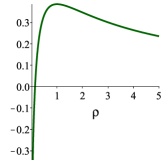
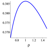
$\varphi(\rho)$, $\rho\in(0,5)$	$\varphi(\rho)$, $\rho\in(0.65,1.5)$

Figure 6. The behaviors of $\varphi(\rho)$.

We first identify $k$ at which $|M_{n,k}|n^{k}$ reaches the maximum value for fixed $n$. We substitute first $k\sim\tau n$, $\tau\in[0,1]$, and $r\sim\rho n$, $\rho>0$, in the saddle-point approximation (21), and obtain, by using (12) and Stirling’s formula:

$$\log\frac{|M_{n,k}|n^{k}}{\beta_{n}} \sim\log(|s_{n,k}|n^{k})\sim\bigl{(}{\log n+\varphi(\rho)}\bigr{)}n,$$

where $\varphi(\rho):=\rho(1-\log\rho)\log(1+\rho^{-1})+\log(1+\rho)-1$, and the pair $(\rho,\tau)$ is connected by the relation $\rho\log(1+\rho^{-1})=\tau$. A simple calculus shows that the image of $\varphi(\rho)$ (see Figure 6) lies in the range $(-\infty,\varphi(1)]$ for $\rho\in(0,\infty)$, where the maximum of $\varphi$ at $\rho=1$ equals $\varphi(1)=2\log 2-1\approx 0.38629\dots$. Then $\rho=1$ implies that $k\sim\mu n$, where $\mu=\log 2$.

Once the peak of $|M_{n,k}|n^{k}$ is identified to be at $k\sim\mu n$, we then refine all the asymptotic expansions by writing $k=\mu n+x\sigma\sqrt{n}$, and then solving the saddle-point equation we obtain

$$r=n+\frac{x\sqrt{n}}{\sigma}+\frac{x^{2}-2\sigma^{2}}{8\sigma^{2}}+\frac{x}{96\sigma^{7}\sqrt{n}}\bigl{(}{12\sigma^{4}-8\sigma^{2}x^{2}-6\sigma^{2}+3x^{2}}\bigr{)}+O\Bigl{(}{\frac{1+x^{4}}{n}}\Bigr{)},$$

whenever $x=o(n^{\frac{1}{6}})$. Substituting this expansion into Moser and Wyman’s saddle-point approximation (21) and using (19), gives the local Gaussian behavior of $|M_{n,k}|n^{k}$:

(22) $$\begin{split}\mathbb{P}(Y_{n}=k)&=\frac{|M_{n,k}|n^{k}}{P_{n}(n)}\\ &=\frac{e^{-\frac{1}{2}x^{2}}}{\sqrt{2\pi\sigma^{2}n}}\Bigl{(}{1+\frac{x((4\sigma^{2}-1)x^{2}-3(2\sigma^{2}-1))}{24\sigma^{3}\sqrt{n}}+O\Bigl{(}{\frac{(1+x^{4})\log n}{n}}\Bigr{)}}\Bigr{)},\end{split}$$

uniformly for $k=\mu n+x\sigma\sqrt{n}$ with $x=o(n^{\frac{1}{6}})$.

When $|x|$ lies outside the central range, say $|x|\geqslant n^{\frac{1}{8}}$ (for simplicity), we use the crude bounds (with $k_{\pm}:=\mu n\pm\sigma n^{\frac{5}{8}}$)

$$\mathbb{P}\bigl{(}{Y_{n}\leqslant k_{-}}\bigr{)}+\mathbb{P}\bigl{(}{Y_{n}\geqslant k_{+}}\bigr{)} =O\biggl{(}{n\max_{|k-\mu n|\geqslant\sigma n^{\frac{5}{8}}}\frac{|s_{n,k}|n^{k}}{n!}}\biggr{)}=O\Bigl{(}{\frac{n|s_{n,k_{-}}|n^{k_{-}}}{n!}}\Bigr{)}=O\bigl{(}{n^{\frac{1}{2}}e^{-\frac{1}{2}n^{\frac{1}{4}}}}\bigr{)},$$

by (22). This together with (22) completes the proof of Theorem 3.

4.5. Three sequences with the same $\mathscr{N}(\mu n,\sigma^{2}n)$ asymptotic distribution

Our proof of Theorem 3 also implies the same local limit theorem (17) for the sequence $|s_{n,k}|n^{k-1}$ (A056856).

Two other OEIS sequences with the same asymptotic behaviors are

• A220883:

  $$[z^{k}]\prod_{1\leqslant j<n}(j+(n+1)z)=|s_{n,k+1}|(n+1)^{k}.$$

• A260887:

  $$[z^{k}]\prod_{2\leqslant j\leqslant n}(j+nz)=n^{k}\sum_{0\leqslant j\leqslant k}|s_{n+1,j+1}|(-1)^{k-j}.$$

The proof of Theorem 3 also extends to these cases; for example, by Moser and Wyman’s saddle-point analysis, we first have

$$[z^{k}]\prod_{2\leqslant j\leqslant n}(j+nz)=\frac{r^{-k}\Gamma(n+1+r)}{\sqrt{2\pi V}\,\Gamma(r+2)}\bigl{(}{1+O\bigl{(}{V^{-1}}\bigr{)}}\bigr{)},$$

where $r>0$ solves the equation $n(\psi(n+r+1)-\psi(r+2))=k$ and $V:=k+r^{2}(\psi^{\prime}(n+r+1)-\psi^{\prime}(r+2))$. Then we follow the same proof of Theorem 3 and obtain, for A260887,

$$\left\{[z^{k}]\prod_{2\leqslant j\leqslant n}(j+nz)\right\}_{k}\simeq\mathrm{LLT}\bigl{(}{\mu n,\sigma^{2}n,n^{-\frac{1}{2}}}\bigr{)},$$

The same result holds for A220883. In contrast, the neighboring sequence A220884

$$[z^{k}]\prod_{2\leqslant j\leqslant n}(j+(n+1-j)z)$$

satisfies $\mathscr{N}(\frac{1}{2}n,\frac{1}{6}n;n^{-\frac{1}{2}})$, which can be proved either by Harper’s real-rootedness approach or the classical characteristic function approach (using Lévy’s continuity theorem); see [18, p. 108].

5. Distribution of Arima numbers

5.1. Yoriyuki Arima and his 1763 book on Bell numbers

Yoriyuki Arima (1714–1783) was born in Kurume Domain and then became the Feudal lord there at the age of 16. As was common at that time, he also used several different names during his life time. He apprenticed himself to Nushizumu Yamaji (山路主住), and later wrote over 40 books during 1745–1766. He selected and compiled 150 typical questions from these books and published the solutions in the compendium book Shuki Sanpo [2] (拾璣算法) in five volumes under the pen-name Bunkei Toyoda (豐田文景). This influential book was regarded highly in Wasan at that time and played a significant role in popularizing the theory and techniques developed in the Seki School. Not only the materials are well-organized, but the style is comprehensible, which is unique and was thought to be a valuable contribution to the developments of Wasan in and after the Edo period. For more information on Arima’s life and mathematical works, see [10].

Our next focus in this paper lies on his 1763 book [1], which is devoted to two different procedures of computing Bell numbers, a summary of which being given as follows.

• Matsunaga’s procedure (2) is first examined (pp. 3–5), and the values of $B_{n}$ for $n=2,\dots,13$ are computed.

• Values of the Matsunaga numbers $M_{n,k}$ are listed on page 6.

• Computing $B_{n}$ through the better recurrence (1) (pp. 7–12), which is simplified with the additional (common) tabular trick (trading off space for computing time) that

  $$b_{n,k}:=\binom{n-1}{k-1}B_{n-k}=\begin{cases}\displaystyle\sum_{1\leqslant j<n}b_{n-1,j},&\text{if }k=1;\\ \displaystyle\frac{n-1}{k-1}\,b_{n-1,k-1},&\text{if }2\leqslant k\leqslant n.\end{cases}$$

  It follows that $B_{n}=\sum_{1\leqslant k\leqslant n}b_{n,k}$.

• Stirling numbers of the first kind $s_{n,k}$ are tabulated for $2\leqslant n\leqslant 10$ (pp. 12–16) via the expansion of $x(x-1)\cdots(x-n+1)$.

• Then the next twenty pages or so (pp. 17–36) give a detailed inductive discussion to compute the number of arrangements when there are $k_{1}$ blocks of size $1$, $k_{2}$ blocks of size $2$, etc. (essentially the coefficients of the Bell polynomials):

  $$B_{n}(k_{1},k_{2},\dots)=\frac{n!}{1!^{k_{1}}2!^{k_{2}}\cdots k_{1}!k_{2}!\cdots}.$$

• Bell numbers are computed (pp. 36–41) by collecting all different block configurations (or adding the coefficients in the Bell polynomials).

• Matsunaga numbers $M_{n,k}$ are computed on pages 42–47, where $\beta_{n}$ is given on page 43.

• The remaining pages (48–55) discuss multinomial coefficients.

5.2. Arima numbers

In this section, for completeness, we prove the LLT of the Arima numbers

$$A_{n,k}:=\binom{n}{k}B_{n-k},$$

which appeared in Arima’s 1763 book (pages 7–8 in file order) and also sequence A056857 in the OEIS; its row-reversed version corresponds to A056860. Since our main interest lies in the asymptotic distribution, we consider $\binom{n}{k}B_{n-k}$ instead of the original $\binom{n-1}{k}B_{n-1-k}$.

Another closely related sequence is A175757 (number of blocks of a given size in set partitions), which is the same as A056857 but without the leftmost column.

Several interpretations or contexts where these sequences arise can be found on the OEIS page; see also [22, p. 178] for the connection to weak records in set partitions. For example, it gives the size of the block containing $1$, as well as the number of successive equalities in set partitions.

On the other hand, the sequence A005578 ($\lceil\frac{1}{3}2^{n}\rceil$) is sometimes referred to as the Arima sequence.

$n\backslash k$	$0$	$1$	$2$	$3$	$4$	$5$	$6$	$7$	$B_{n+1}$
$1$	$1$	$1$							$2$
$2$	$2$	$2$	$1$						$5$
$3$	$5$	$6$	$3$	$1$					$15$
$4$	$15$	$20$	$12$	$4$	$1$				$52$
$5$	$52$	$75$	$50$	$20$	$5$	$1$			$203$
$6$	$203$	$312$	$225$	$100$	$30$	$6$	$1$		$877$
$7$	$877$	$1421$	$1092$	$525$	$175$	$42$	$7$	$1$	$4140$

Table 3. The values of $A_{n,k}$ for $n=1,\dots,7$ and $1\leqslant k\leqslant n$ as already given on [1, Page 8].

Theorem 4.

(23) $$\left\{\binom{n}{k}B_{n-k}\right\}_{k}\,\simeq\,\mathrm{LLT}\bigl{(}{\log n,\log n;(\log n)^{-\frac{1}{2}}}\bigr{)}.$$

The same LLT holds for the sequence A175757, and for A056860, we have

$$\left\{\binom{n}{k}B_{k}\right\}_{k}\,\simeq\,\mathrm{LLT}\bigl{(}{n-\log n,\log n;(\log n)^{-\frac{1}{2}}}\bigr{)}.$$

Proof.

Recall first the known saddle-point approximation to Bell numbers (see [8, 27])

(24) $$\begin{split}B_{n}&=n![z^{n}]e^{e^{z}-1}\\ &=\frac{e^{(w+\frac{1}{w}-1)n-1}}{\sqrt{w+1}}\Bigl{(}{1-\frac{w^{2}(2w^{2}+7w+10)}{24n(w+1)^{3}}+O\bigl{(}{n^{-2}(\log n)^{2}}\bigr{)}}\Bigr{)}.\end{split}$$

where $w=W(n)$. From this and the asymptotic expansion (15), we can quickly see why (23) holds. Since $\binom{n}{k}<2^{n}$ for all $k$, and $\log B_{n}\sim nw\sim n\log n-n\log\log n$, meaning that $B_{n}$ is very close to factorial, and thus larger than the binomial term. The largest term of $B_{n-k}$ is when $k=0$. More precisely, when $k$ is small,

(25) $$\binom{n}{k}\frac{B_{n-k}}{B_{n}}\sim\frac{n^{k}}{k!}\times n^{-k}(\log n)^{k}=\frac{(\log n)^{k}}{k!},$$

and thus a CLT with logarithmic mean and logarithmic variance is naturally expected.

For a rigorous proof, we begin with the calculation of the mean. First,

$$A_{n,k}=n![z^{n}v^{k}]e^{e^{z}-1+vz},$$

and from this exponential generating function, we can derive the (exact) mean and the variance to be

$$\mu_{n}:=\frac{nB_{n}}{B_{n+1}},\quad\text{and}\quad\sigma_{n}^{2}:=\frac{n(n-1)B_{n-1}+nB_{n}}{B_{n+1}}-\Bigl{(}{\frac{nB_{n}}{B_{n+1}}}\Bigr{)}^{2},$$

respectively. The asymptotic mean and variance then follow from (24) and the asymptotic expansion (15); indeed, finer expansions give

$$\mu_{n} =w\Bigl{(}{1-\frac{w^{2}}{2n(w+1)^{2}}+O\bigl{(}{n^{-2}(\log n)^{2}}\bigr{)}}\Bigr{)},$$

$$\sigma_{n}^{2} =w\Bigl{(}{1-\frac{w(3w+2)}{2n(w+1)^{2}}+O\bigl{(}{n^{-2}(\log n)^{2}}\bigr{)}}\Bigr{)}.$$

An alternative approach by applying saddle-point method and Quasi-powers theorem [17, 9] is as follows. First, we derive, again by saddle-point method, the asymptotic approximation

$$n![z^{n}]e^{e^{z}-1+vz} =\frac{n!}{2\pi i}\oint_{|z|=r}z^{-n-1}e^{e^{z}-1+vz}{\,\rm d}z$$

$$=\frac{n!r^{-n}e^{\frac{n}{r}-1+vr}}{\sqrt{2\pi((r+1)n-vr^{2})}}\bigl{(}{1+O\bigl{(}{rn^{-1}}\bigr{)}}\bigr{)},$$

uniformly for complex $v$ in a small neighborhood of unity $|v-1|=o(1)$, where $r=r(v)>0$ solves the equation $re^{r}+vr=n$. For large $n$, a direct bootstrapping argument gives the asymptotic expansion

$$r=w-\frac{vw^{2}}{n(w+1)}-\frac{v^{2}w^{3}(w^{2}-2)}{2n^{2}(w+1)^{3}}+O\bigl{(}{n^{-3}(\log n)^{3}}\bigr{)},$$

uniformly for bounded $v$. From these expansions, we then obtain

$$\frac{n![z^{n}]e^{e^{z}-1+vz}}{n![z^{n}]e^{e^{z}-1+z}}=e^{w(v-1)}\bigl{(}{1+O\bigl{(}{n^{-1}\log n}\bigr{)}}\bigr{)},$$

uniformly for $|v-1|=o(1)$. This implies an asymptotic Poisson($W(n)$) distribution for the underlying random variables, and, in particular, the CLT $\mathscr{N}(\log n,\log n)$ follows. The stronger LLT (23) is proved by (24) and standard approximations for binomial coefficients, following the same procedure used in the proof of (17); in particular, we use the expansion of $\binom{n}{k}$:

$$\binom{n}{k}=\frac{\tau^{-\tau n}(1-\tau)^{-(1-\tau)n}}{\sqrt{2\pi\tau(1-\tau)n}}\Bigl{(}{1+O\bigl{(}{k^{-1}+(n-k)^{-1}}\bigr{)}}\Bigr{)},$$

holds uniformly as $k,n-k\to\infty$, where $\tau=k/n$. Outside this range, $\binom{n}{k}B_{n-k}$ is asymptotically negligible. ∎

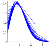
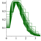
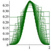
$\frac{\binom{n}{x\log n}B_{n-x\log n}}{\sum_{1\leqslant j\leqslant n}\binom{n}{j}B_{n-j}}$	$\frac{\binom{n}{\left\lfloor x\log n\right\rfloor}B_{n-\left\lfloor x\log n\right\rfloor}}{\sum_{1\leqslant j\leqslant n}\binom{n}{j}B_{n-j}}$	$\frac{\binom{n}{xn}B_{xn}B_{n-xn}}{\sum_{1\leqslant j\leqslant n}\binom{n}{j}B_{j}B_{n-j}}$	$\frac{\binom{n}{\lfloor{\frac{1}{2}xn\rfloor}}B_{\lfloor{\frac{1}{2}xn\rfloor}}B_{n-\lfloor{\frac{1}{2}xn\rfloor}}}{\sum_{1\leqslant j\leqslant n}\binom{n}{j}B_{j}B_{n-j}}$
$n=2\ell,1\leqslant\ell\leqslant 25$	$n=2\ell+1,2\leqslant\ell\leqslant 24$		$n=2\ell+1,1\leqslant\ell\leqslant 29$

Figure 7. Histograms of Arima numbers $\binom{n}{k}B_{n-k}$ (the left two plots) and the sequence $\binom{n}{k}B_{k}B_{n-k}$ (A033306; the right two plots). All plots, except for the third one, are scaled by the standard deviations.

5.3. Asymptotic normality of a few variants

A few other distributions with the same logarithmic type LLT are listed in Table 4, the proofs being completely similar and omitted.

OEIS	A078937	A078938	A078939	A124323	A086659
EGF	$e^{2(e^{z}-1)+vz}$	$e^{3(e^{z}-1)+vz}$	$e^{4(e^{z}-1)+vz}$	$e^{e^{z}-1+(v-1)z}$	$e^{e^{z}-1+(v-1)z}-e^{vz}$

Table 4. A few OEIS sequences (together with their EGFs) with the same $\mathrm{LLT}\bigl{(}{\log n,\log n;(\log n)^{-\frac{1}{2}}}\bigr{)}$ asymptotic behavior as Arima numbers.

In particular, A124323 enumerates singletons in set partitions.

These EGFs are reminiscent of $r$-Bell numbers with the EGF $e^{v(e^{z}-1)+rz}$ [6, 26]; see also [13] for exponential Riordan arrays of the type $e^{(\alpha+v)(e^{z}-1)+(\alpha-\beta)z}$. These types of EGFs lead however to normal limit laws with mean of order $\frac{n}{W(\frac{n}{\alpha+1})}$ and variance of order $\frac{n}{W(\frac{n}{\alpha+1})}$ when $\alpha>0$ and $\beta\leqslant 2\alpha$, and of order $\frac{n}{W(n)^{2}}$ when $\alpha=0$ and $\beta\leqslant 0$, similar to that of $\genfrac{\{}{\}}{0.0pt}{}{n}{k}$.

5.4. A less expected $\mathrm{LLT}(\frac{1}{2}n,\frac{1}{4}n\log n)$ for $\binom{n}{k}B_{k}B_{n-k}$

On the other hand, from the intuitive reasoning given in (25) (which can be made rigorous), it is of interest to scrutinize the corresponding balanced version $\binom{n}{k}B_{k}B_{n-k}$, which is sequence A033306 with the EGF $e^{e^{vz}+e^{z}-2}$. In this case, the peak of the distribution is reached at $k=\left\lfloor\frac{1}{2}n\right\rfloor$ and $k=\lceil\frac{1}{2}n\rceil$. Indeed, the mean is identically $\frac{1}{2}n$, and the variance can be computed by

$$\frac{n}{4}+\frac{n(n-1)\tilde{B}_{n-1}}{4\tilde{B}_{n}},$$

where $\tilde{B}_{n}:=n![z^{n}]e^{2(e^{z}-1)}$ is sequence A001861 in the OEIS (or the $n$th moment of a Poisson distribution with mean $2$). By the asymptotic expansion ($\tilde{w}:=W(\frac{1}{2}n)$)

(26) $$\tilde{B}_{n}=\frac{e^{(\tilde{w}-1+\log 2+\tilde{w}^{-1})n-2}}{\sqrt{\tilde{w}+1}}\Bigl{(}{1-\frac{\tilde{w}^{2}(2\tilde{w}^{2}+7\tilde{w}+10)}{24(\tilde{w}+1)^{3}n}+O\bigl{(}{n^{-2}(\log n)^{2}}\bigr{)}}\Bigr{)},$$

we have that the variance satisfies

$$\frac{n}{4}+\frac{n(n-1)\tilde{B}_{n-1}}{4\tilde{B}_{n}}=\frac{\tilde{w}+1}{4}\,n-\frac{\tilde{w}(\tilde{w}^{2}+2\tilde{w}+2)}{8(\tilde{w}+1)^{2}}+O\bigl{(}{n^{-1}(\log n)^{2}}\bigr{)},$$

showing the less expected $n\log n$ asymptotic behavior. By (26) and Stirling’s formula, we obtain, for $k=\frac{1}{2}n+\frac{1}{2}x\sqrt{n(\tilde{w}+1)}$,

$$\frac{\binom{n}{k}B_{k}B_{n-k}}{\tilde{B}_{n}}=\frac{e^{-\frac{1}{2}x^{2}}}{\sqrt{\frac{1}{2}\pi n(\tilde{w}+1)}}\Bigl{(}{1+O\Bigl{(}{\frac{\log n}{n}(1+x^{4})}\Bigr{)}}\Bigr{)},$$

uniformly in the range $x=o(n^{\frac{1}{4}}(\log n)^{\frac{1}{4}})$ (wider than the usual range $o(n^{\frac{1}{6}})$ due to symmetry of the distribution). Smallness of the distribution outside this range also follows from similar arguments, and we deduce that

$$\binom{n}{k}B_{k}B_{n-k}\simeq\mathrm{LLT}\Bigl{(}{\frac{n}{2},\frac{n\tilde{w}}{4};\frac{\log n}{n}}\Bigr{)}.$$

Finally, sequence A174640, which equals $\binom{n}{k}B_{k}B_{n-k}-B_{n}+1$ also follows asymptotically the same behaviors.

6. Conclusions

We clarified the two Edo-period procedures in the eighteenth century in Japan to compute Bell numbers, and derived fine asymptotic and distributional properties of several classes of numbers arising in such procedures, shedding new light on the early history and developments of Bell and related numbers.

In addition to the modern perspectives given in this paper, our study of these old materials also suggests several other questions. For example, the change of the asymptotic distributions from $\mathrm{LLT}(\log n,\log n)$ for $|M_{n,k}|$ to $\mathrm{LLT}(\mu n,\sigma^{2}n)$ for $|M_{n,k}|n^{k}$ suggests examining other weighted cases, say $\binom{n}{k}|M_{n,k}|$ or more generally $\pi_{n,k}|M_{n,k}|$ for a given sequence $\pi_{n,k}$, and studying the corresponding phase transitions of limit laws. This and several related questions will be explored in detail elsewhere.

References

- [1] Y. Arima. Danren Henkyokuhō (断連変局法, Variational Techniques of Separate-and-Link). 1763.
- [2] Y. Arima. Shūki Sanpō (拾璣算法, Collections in Arithmetics). Senjubo Publisher, 1769.
- [3] H. W. Becker and J. Riordan. The arithmetic of Bell and Stirling numbers. Amer. J. Math., 70:385–394, 1948.
- [4] E. T. Bell. The iterated exponential integers. Ann. of Math. (2), 39(3):539–557, 1938.
- [5] E. A. Bender. Central and local limit theorems applied to asymptotic enumeration. J. Combinatorial Theory Ser. A, 15:91–111, 1973.
- [6] A. Z. Broder. The -Stirling numbers. Discrete Math., 49(3):241–259, 1984.
- [7] R. M. Corless, G. H. Gonnet, D. E. G. Hare, D. J. Jeffrey, and D. E. Knuth. On the Lambert function. Adv. Comput. Math., 5(4):329–359, 1996.
- [8] N. G. de Bruijn. Asymptotic Methods in Analysis. Dover Publications, Inc., New York, third edition, 1981.
- [9] P. Flajolet and R. Sedgewick. Analytic Combinatorics. Camb. Univ. Press, 2009.
- [10] M. Fujiwara, editor. History of Mathematics in Japan before Meiji (Japan Academy), volume 2. Iwanami, Tokyo, 1957.
- [11] H. W. Gould. Catalan and Bell numbers: Research bibliography of two special number sequences. Published by the author, 1979.
- [12] T. Hayashi. On the combinatory analysis in the old Japanese mathematics. Tohoku Math. J., First Series, 33:328–365, 1931.
- [13] A. Hennessy and P. Barry. Generalized Stirling numbers, exponential Riordan arrays and orthogonal polynomials. J. Integer Seq., 14:11–8, 2011.
- [14] A. Hirayama. Yoshisuke Matsunaga (松永良弼). Tokyo Horei Publishing Co., 1987.
- [15] H.-K. Hwang. Théorèmes limites pour les structures combinatoires et les fonctions arithmétiques. PhD thesis, LIX, École polytechnique, Palaiseau, France, December 1994.
- [16] H.-K. Hwang. Asymptotic expansions for the Stirling numbers of the first kind. J. Combinatorial Theory Ser. A, 71(2):343–351, 1995.
- [17] H.-K. Hwang. On convergence rates in the central limit theorems for combinatorial structures. European J. Combin., 19(3):329–343, 1998.
- [18] H.-K. Hwang, H.-H. Chern, and G.-H. Duh. An asymptotic distribution theory for Eulerian recurrences with applications. Adv. in Appl. Math., 112:101960, 125, 2020.
- [19] D. E. Knuth. Two notes on notation. Amer. Math. Monthly, 99:403–422, 1992.
- [20] D. E. Knuth. The Art of Computer Programming. Vol. 4A. Combinatorial Algorithms. Part 1. Addison-Wesley, Upper Saddle River, NJ, 2011.
- [21] P. Luschny. Set partitions and Bell numbers.
- [22] T. Mansour. Combinatorics of Set Partitions. CRC Press Boca Raton, 2013.
- [23] T. Mansour and M. Schork. Commutation Relations, Normal Ordering, and Stirling Numbers. CRC Press, Boca Raton, FL, 2016.
- [24] Y. Matsunaga. Danren Sōjutsu (断連総術, General Techniques of Separate-and-Link). 1726.
- [25] N. S. Mendelsohn and J. Riordan. Problem 4340 and solution. Amer. Math. Monthly, 58:46–48, 1951.
- [26] I. Mező. The -Bell numbers. J. Integer Seq., 14(1):Article 11.1.1, 14, 2011.
- [27] L. Moser and M. Wyman. An asymptotic formula for the Bell numbers. Trans. Roy. Soc. Canada Sect., 49:49–54, 1955.
- [28] L. Moser and M. Wyman. Asymptotic development of the Stirling numbers of the first kind. J. London Math. Soc., 33:133–146, 1958.
- [29] OEIS Foundation Inc. The On-Line Encyclopedia of Integer Sequences.
- [30] A. I. Pavlov. Local limit theorems for the number of components of random permutations and mappings. Theory Probab. Appl., 33(1):183–187, 1989.
- [31] S. Pollard. C. S. Peirce and the Bell Numbers. Math. Mag., 76(2):99–106, 2003.
- [32] G.-C. Rota. The number of partitions of a set. Amer. Math. Monthly, 71:498–504, 1964.
- [33] T. Seki. Katsuyō Sanpō (括要算法, Compendium of Arithmetics). 1712.
- [34] N. M. Temme. Asymptotic estimates of Stirling numbers. Stud. Appl. Math., 89:233–243, 1993.