Abstract

Consider the rank-1 spiked model: ${\mathbf{X}=\sqrt{\nu}\xi\mathbf{u}+\mathbf{Z}}$, where $\nu$ is the spike intensity, $\mathbf{u}\in\mathbb{S}^{k-1}$ is an unknown direction and ${\xi\sim\mathcal{N}(0,1),\mathbf{Z}\sim\mathcal{N}(\bm{0},\bm{I})}$. Motivated by recent advances in analog-to-digital conversion, we study the problem of recovering $\mathbf{u}\in\mathbb{S}^{k-1}$ from $n$ i.i.d. modulo-reduced measurements $\mathbf{Y}=[\mathbf{X}]\mod\Delta$, focusing on the high-dimensional regime ($k\gg 1$). We develop and analyze an algorithm that, for most directions $\mathbf{u}$ and $\nu=\mathrm{poly}(k)$, estimates $\mathbf{u}$ to high accuracy using $n=\mathrm{poly}(k)$ measurements, provided that $\Delta\gtrsim\sqrt{\log k}$. Up to constants, our algorithm accurately estimates $\mathbf{u}$ at the smallest possible $\Delta$ that allows (in an information-theoretic sense) to recover $\mathbf{X}$ from $\mathbf{Y}$. A key step in our analysis involves estimating the probability that a line segment of length $\approx\sqrt{\nu}$ in a random direction $\mathbf{u}$ passes near a point in the lattice $\Delta\mathbb{Z}^{k}$. Numerical experiments show that the developed algorithm performs well even in a non-asymptotic setting.

1 Introduction

We consider the problem of estimating a spiked covariance matrix from Gaussian modulo-folded measurements. Let $\mathbf{u}\in\mathbb{S}^{k-1}$ be an unknown direction, and $\nu>0$ be the signal-to-noise (SNR) ratio. Consider the spiked covariance matrix

$${\bf{\Sigma}}=\nu\mathbf{u}\mathbf{u}^{\top}+\bm{I}\,,$$ (1)

and denote $\mathbf{X}\sim\mathcal{N}(\bm{0},{\bf{\Sigma}})$. Equivalently, one may write

$$\mathbf{X}=\sqrt{\nu}\xi\mathbf{u}+\mathbf{Z}\,,$$ (2)

where $\xi,\mathbf{Z}$ have $\mathcal{N}(0,1)$ entries; the one dimensional component $\sqrt{\nu}\xi\mathbf{u}$ is often thought of as the “signal”, whereas $\mathbf{Z}$ is thought of as “noise”. In this paper, we consider the problem of estimating $\mathbf{u}$ from $n$ independent and modulo-reduced measurements of $\mathbf{X}$. Let $\Delta>0$ be the dynamic range, and for ${X\in\mathbb{R}}$, denote the modulo operation by

$$Y=[X]\bmod\Delta\in\left[-\frac{1}{2}\Delta,\frac{1}{2}\Delta\right)\,,$$ (3)

so that $Y$ is the unique number in the half-open interval such that $X-Y\in\Delta\mathbb{Z}$. For a vector ${\mathbf{X}\in\mathbb{R}^{k}}$, $\mathbf{Y}=[\mathbf{X}]\bmod\Delta$ is defined by modulo-reducing each coordinate separately. In the setup we consider, one is given $n$ independent copies of $\mathbf{Y}$, denoted by $\mathbf{y}_{1},\ldots,\mathbf{y}_{n}$, and wishes to estimate the unknown direction $\mathbf{u}\in\mathbb{S}^{k-1}$. Throughout, we denote by $\mathbf{x}_{1},\ldots,\mathbf{x}_{n}$ independent copies of $\mathbf{X}$, such that $\mathbf{y}_{i}=[\mathbf{x}_{i}]\bmod\Delta$. See Figure 1 for a graphical illustration, in $k=2$ dimensions.

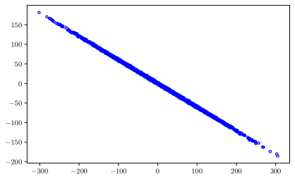
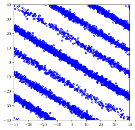
Figure 1: A typical problem instance in $k=2$ dimensions. Top: A point cloud, corresponding to $n=5000$ i.i.d. samples from $\mathbf{X}\sim\mathcal{N}(\bm{0},\nu\mathbf{u}\mathbf{u}^{\top}+\bm{I})$, for $\nu=10^{4}$ and some fixed $\mathbf{u}\in\mathbb{S}^{k-1}$. Bottom: The modulo-reduced point cloud, with $\Delta=80$.

Motivation.

Our motivation for considering this problem is driven by recent developments in signal processing. Analog-to-digital converters (ADCs), devices that convert analog (continuous) signals into digital (discrete, e.g. bits) signals, are an essential component in virtually all modern communication devices. From a mathematical perspective, ADCs are set out to solve essentially the following problem: Given a vector-valued random variable $\mathbf{X}\in\mathbb{R}^{k}$, find a quantizer (binning scheme), $\phi:\mathbb{R}^{k}\to\mathbb{R}^{k}$, with a finite range, $|\mathrm{range}(\phi)|\leq 2^{B}$ ($B$ being the allowable representation length in bits), so as to minimize the quantization error: $\mathbb{E}\|\mathbf{X}-\phi(\mathbf{X})\|^{2}$. Quantization is an extensively studied problem, and its fundamentals limits (in information theory: “rate-distortion theory”), under setups of varying generality, are largely understood; see, e.g., [Cover and Thomas, 2012, Gersho and Gray, 2012].

Optimal vector quantizers (that achieve the fundamental limits) typically involve rather complicated constructions, that depend intricately on the exact statistics of $\mathbf{X}$. Since ADCs are implemented in mixed analog-digital circuits, sophisticated vector quantizers are prohibitive and the design is often restricted to architectures of a scalar product form: ${\phi(\mathbf{X})=(\phi_{1}(X_{1}),\ldots,\phi_{k}(X_{k}))}$ where ${\phi_{1},\ldots,\phi_{k}:\mathbb{R}\to\mathbb{R}}$. Perhaps the simplest – and most popular – architecture in practice is a uniform scalar quantizer, determined by its dynamic range $\Delta>0$ and bit-rate $b=B/k$. The quantizer divides the interval $[-\Delta/2,\Delta/2]$ into $2^{b}$ intervals of equal size $\Delta 2^{-b}$, so that the scalar quantizer $\phi_{1}=\ldots=\phi_{k}=\phi$ maps $X\in\mathbb{R}$ to its closest interval center. Note that for this scheme to attain quantization error that vanishes as the quantization rate $b$ increases, the dynamic range must be $\Delta\gtrsim\max_{1\leq i\leq k}\sqrt{\mathrm{Var}(X_{i})}$.

Although simple to implement, the uniform quantizer can be pronouncedly sub-optimal for vector-valued signals, as it cannot leverage the cross-coordinate correlations that often occur in real-world applications. An important use-case in digital communications is Massive MIMO, where typically the number of users is much smaller than the number of receive antennas; this results in signals $\mathbf{X}$ that have strong cross-entry correlations. Thus, a quantization scheme that can exploit these statistical inter-dependencies, while retaining the simplicity of the uniform quantizer, is highly desired.

A recently proposed architecture, “modulo-ADCs” [Ordentlich et al., 2018], attempts to address these issues. Their idea is rather simple: do not truncate $\mathbf{X}$ onto $[-\Delta/2,\Delta/2]^{k}$, as the uniform quantizer does; instead, apply modulo-reduction $\mathbf{Y}=[\mathbf{X}]\bmod\Delta\in[-\Delta/2,\Delta/2]^{k}$ and then quantize as before. For this idea to work, one clearly need some means of “unwrapping” $\mathbf{X}$ from $\mathbf{Y}$ (with high probability). When the coordinates of $\mathbf{X}$ are independent and unimodal, with the mode at $0$ (for example, a centered Gaussian), it is easy to see that the best estimator for $\mathbf{X}$ from $\mathbf{Y}$ (in the sense of error probability) is just $\widehat{\mathbf{X}}=\mathbf{Y}$. Thus, a coordinate $X_{i}$ cannot be recovered once it saturates the ADC dynamic range, $|X_{i}|\geq\Delta/2$; so to consistently undo the modulo, one needs $\Delta\gtrsim\max_{1\leq i\leq k}\sqrt{\mathrm{Var}(X_{i})}$, and the scheme has no advantage over the standard uniform quantizer. It turns out, however, that when $\mathbf{X}$ has strong correlations, it is often possible to consistently unwrap at substantially smaller values of $\Delta$; see next section.

1.1 Related work

We start with very brief background on the spiked model, Eq. (2). In the high-dimensional statistics ($k\approx n$, $k,n\to\infty$) literature, the spiked model was popularized by [Johnstone, 2001], who studied the largest eigenvalue of the sample covariance matrix $\widehat{{\bf{\Sigma}}}=\frac{1}{n}\sum_{i=1}^{n}\mathbf{x}_{i}\mathbf{x}_{i}^{\top}$. Subsequent advances in random matrix theory [Baik et al., 2005, Paul, 2007] characterized the behavior of PCA (namely, the relation between the principal components of ${\bf{\Sigma}}$ and its empirical counterpart $\widehat{{\bf{\Sigma}}}$) rather precisely. Since then, a vast literature on the spiked model (and variations thereof) has emerged – which we make no pretense to survey here; as an entry point, geared towards statisticians, see [Wainwright, 2019, Chapter 8]. We cite the following minimax lower bound for the spike estimation problem (without modulo-reduction) [Wainwright, 2019, Example 15.19]:

$$\left\|\mathbf{u}-\widehat{\mathbf{u}}\right\|\gtrsim\left(\frac{\sqrt{1+\nu}}{\nu}\sqrt{\frac{k}{n}}\right)\wedge 1\,.$$ (4)

In the regime $k=O(n)$, this rate is attained, up to prefactors, by PCA ($\widehat{\mathbf{u}}$ taken to be the largest eigenvector of $\widehat{{\bf{\Sigma}}}$), see [Wainwright, 2019, Corollary 8.7].

Moving on, there has recently been a great deal of activity in the signal processing community around recovery from modulo-reduced measurements [Bhandari et al., 2017, Ordentlich et al., 2018, Bhandari et al., 2018, Graf et al., 2019, Romanov and Ordentlich, 2019, Bhandari and Krahmer, 2019, Bhandari et al., 2020, Bhandari et al., 2021, Weiss et al., 2021]. Most relevant to this paper is a line of works dealing with recovery from modulo-reduced measurements, and motivated by the modulo-ADC architecture described before [Ordentlich and Erez, 2017, Ordentlich et al., 2018]. The setting is this: the source is Gaussian $\mathbf{X}\sim\mathcal{N}(\bm{0},{\bf{\Sigma}})$, with ${\bf{\Sigma}}$ some covariance matrix (not necessarily spiked); one observes modulo-reduced measurements $\mathbf{Y}=[\mathbf{X}]\mod\Delta$, and wishes to recover $\mathbf{X}$ itself (with high probability). How large should $\Delta$ be so that consistent recovery is possible, in an information-theoretic sense? When it is possible, how could one do so practically? (Assuming ${\bf{\Sigma}}$ is known? And when it is not?) The answers, it turns out, depend rather intricately on the diophantine properties of the matrix ${\bf{\Sigma}}$.

Let us start with the fundamental limits. A simple observation is that when $\Delta\gtrsim\sqrt{\log k}\cdot\max_{1\leq\ell\leq k}\sqrt{{\bf{\Sigma}}_{\ell,\ell}}$ (${\bf{\Sigma}}_{\ell,\ell}$ being the variance of the $\ell$-th coordinate), one has $\mathbf{X}=\mathbf{Y}$ with high probability, so that consistent recovery is straightforward. It is easy to see that when $\mathbf{X}$ is white, in other words ${\bf{\Sigma}}\propto\bm{I}$, this requirement is in fact tight. For general ${\bf{\Sigma}}$, one may readily show that the maximum a posteriori probability (MAP) estimator for $\mathbf{X}$ given $\mathbf{Y}$ is

$$\widehat{\mathbf{X}}_{\mathrm{MAP}}(\mathbf{Y}=\mathbf{y})=\operatorname*{\arg\!\min}_{\mathbf{x}\,:\,\mathbf{x}-\mathbf{y}\in\Delta\mathbb{Z}^{k}}\mathbf{x}^{\top}{\bf{\Sigma}}^{-1}\mathbf{x}\,,$$ (5)

that is, one needs to minimize a quadratic form over the coset of $\mathbf{y}$. Searching over the coset directly (and consequently, computing $\widehat{\mathbf{X}}_{\mathrm{MAP}}$ exactly) is not computationally tractable, in all but the simplest cases; nonetheless, since $\widehat{\mathbf{X}}_{\mathrm{MAP}}$ is optimal in the sense of error probability, its performance characterizes the information-theoretic limits of the problem. The latter has a rather elegant geometric interpretation. Let $\mathcal{L}=\Delta{\bf{\Sigma}}^{-1/2}\mathbb{Z}^{k}\subseteq\mathbb{R}^{k}$ be the lattice generated by $\Delta{\bf{\Sigma}}^{-1/2}\in\mathbb{R}^{k\times k}$, and let $V_{0}\subseteq\mathbb{R}^{k}$ be the Voronoi cell of $\bm{0}\in\mathcal{L}$. Then [Romanov and Ordentlich, 2021] the success probabililty of (5) is the Gaussian measure of $V_{0}$:

$$p_{\mathrm{MAP}}=\Pr\left(\widehat{\mathbf{X}}_{\mathrm{MAP}}=\mathbf{X}\right)=\Pr_{\mathbf{Z}\sim\mathcal{N}(\bm{0},\bm{I})}(\mathbf{Z}\in V_{0})\,.$$

As a corollary, it is not hard to show that $\Delta\lesssim|{\bf{\Sigma}}|^{1/2k}$ implies that $p_{\mathrm{MAP}}=o(1)$; see also Proposition 2. When the lattice $\mathcal{L}$ is a uniformly random lattice, sampled, up to normalization, from the Haar measure over $\faktor{\mathrm{SL}_{k}(\mathbb{R})}{\mathrm{SL}_{k}(\mathbb{Z})}$ (also called Haar-Siegel measure), one can show that $V_{0}$ is with high probability “sufficiently ball-like”, so that $\Delta\gtrsim|{\bf{\Sigma}}|^{1/2k}$ is also a sufficient condition. Random lattices have played a prominent role in the lattice coding literature [Zamir, 2014], which is closely related to the present line of work. An important point is that “natural” random matrix ensembles, such as the spiked ensemble (1) with $\mathbf{u}\sim\mathrm{Unif}(\mathbb{S}^{k-1})$, do not correspond to the Siegel-Haar measure on the space of lattices. In [Domanovitz and Erez, 2017] the authors demonstrate that certain orthogonally-invariant ensembles, that arise in channel coding theory, indeed allow for consistent recovery with $\Delta$ not much larger than $|{\bf{\Sigma}}|^{1/2k}$. In particular, for the spiked ensemble (1), they show that with high probability over $\mathbf{u}\sim\mathrm{Unif}(\mathbb{S}^{k-1})$, the error probability is small whenever $\Delta\gtrsim C(k)|{\bf{\Sigma}}|^{1/2k}=C(k)(1+\nu)^{1/2k}$, where $C(k)$ grows exponentially fast in $k$, but does not depend on the SNR $\nu$.

As for practical recovery algorithms, let us start by assuming ${\bf{\Sigma}}$ is known. As already mentioned, computing the MAP estimator directly is intractable; instead [Ordentlich and Erez, 2017] proposed to use a sub-optimal estimator, the so-called Integer Forcing (IF) decoder. The idea is to find an invertible integer matrix $\mathbf{A}=\left[\mathbf{a}_{1},\ldots,\mathbf{a}_{k}\right]$ so as to minimize the maximal variance:

$$\mathbf{A}_{\mathrm{IF}}=\operatorname*{\arg\!\min}_{\begin{subarray}{c}\mathbf{A}\in\mathbb{Z}^{k\times k},\\ \mathop{\mathrm{rank}}(\mathbf{A})=k\end{subarray}}\max_{1\leq\ell\leq k}{\mathbf{a}_{\ell}^{\top}{\bf{\Sigma}}\mathbf{a}_{\ell}}\,.$$ (6)

The corresponding maximal deviation, $m_{k}({\bf{\Sigma}})=\max_{1\leq\ell\leq k}\sqrt{\mathbf{a}_{\ell}^{\top}{\bf{\Sigma}}\mathbf{a}_{\ell}}$, is called the $k$th successive minimum of the lattice ${\bf{\Sigma}}^{1/2}\mathbb{Z}^{k}$. Since $[\mathbf{A}\mathbf{Y}]\bmod\Delta=[\mathbf{A}\mathbf{X}]\bmod\Delta$, one can reliably recover $\mathbf{X}$ from $\mathbf{Y}$, using $\widehat{\mathbf{X}}_{\mathrm{IF}}=\mathbf{A}_{\mathrm{IF}}^{-1}\left([\mathbf{A}_{\mathrm{IF}}\mathbf{Y}]\mod\Delta\right)$, whenever $\Delta\gtrsim m_{k}({\bf{\Sigma}})\sqrt{\log k}$. Of course, to compute the IF decoder, Eq. (6), one clearly needs to know ${\bf{\Sigma}}$. In some applications, for example in wireless communications (where ${\bf{\Sigma}}$ depends on the channel matrix, which rapidly changes over time) [Tse and Viswanath, 2005], this is not a reasonable assumption. In [Romanov and Ordentlich, 2021], the authors propose a blind unwrapping algorithm, that does not know ${\bf{\Sigma}}$ beforehand, in a setting where one needs to simultaneously unwrap many i.i.d. signals $\mathbf{y}_{1},\ldots,\mathbf{y}_{n}$. A natural step towards that end is to estimate ${\bf{\Sigma}}$ from the (modulo-reduced) data, from which the integer-forcing decoder (6) could be computed. Alas, directly computing the maximum likelihood estimator (MLE) of ${\bf{\Sigma}}$ from modulo-reduced measurements is not computationally feasible. Instead, they propose an algorithm which iteratively alternates between 1) A covariance estimation step, where a certain “proxy” of ${\bf{\Sigma}}$ is estimated; 2) An integer forcing decoder, computed from that proxy; the idea is to gradually “whiten” the entire dataset, effectively computing the IF decoder “in small steps”. They prove a result of the following form: when the error of the informed IF decoder (Eq. (6)) is small enough, then the error of the adaptive algorithm is essentially comparable to it, up to dimension-dependent prefactors. However, their algorithm is only suited to rather modest $k$, as seen both in the analysis (the prefactors are exponential in $k$) and the numerical experiments. The problem lies with their covariance estimation procedure, whose performance breaks down rapidly as the dimension increases. This is the starting point for the present paper.

Our contributions.

We propose a computationally tractable algorithm to estimate the spike ${\mathbf{u}\in\mathbb{S}^{k-1}}$ from modulo-reduced measurements, under the spiked covariance model Eq. (1) and in high dimension $k$. We show that for most directions $\mathbf{u}$ (formally: with high probability over ${\mathbf{u}\sim\mathrm{Unif}(\mathbb{S}^{k-1})}$), estimation is possible with $n=\mathrm{poly}(k)$ samples, under essentially the smallest $\Delta$ (up to constants) that allows for consistent unwrapping. Thus, in this setting, we provably overcome the curse of dimensionality suffered by the algorithm of [Romanov and Ordentlich, 2021]. While we do not directly tackle the unwrapping problem, note that in applications where the SNR $\nu$ is approximately known, the algorithm readily yields an estimate for ${\bf{\Sigma}}$, from whence one could compute the IF decoder (6). Our numerical experiments below show that this method attains an unwrapping error probability that is not far from that of the informed IF decoder.

Notation.

For sequences $a_{k},b_{k}$ we use the following standard notation: $a_{k}\vee b_{k}=\max\{a_{k},b_{k}\}$, $a_{k}\wedge b_{k}=\min\{a_{k},b_{k}\}$. By $a_{k}\lesssim b_{k}$ we mean that $a_{k}\leq Cb_{k}$ for some universal constant $C>0$; we write $a_{k}\approx b_{k}$ whenever both $a_{k}\lesssim b_{k}$ and $b_{k}\lesssim a_{k}$. We also use big-O notation; if $M$ is a parameter, we use $a_{k}=O_{M}(b_{k})$ to signify that the constants might depend on $M$. For a vector $\mathbf{v}\in\mathbb{R}^{k}$, $\|\mathbf{v}\|$ denotes its $\ell_{2}$ (Euclidean) norm.

2 Proposed method

An observation.

Our algorithm is based on the following observation: the eigen-structure of the covariance matrix of $\mathbf{X}$ is preserved when truncated onto a ball. Set $R>0$ a truncation radius. For ${\mathbf{X}\sim\mathcal{N}(\bm{0},{\bf{\Sigma}})}$, let $\mathbf{X}_{\mathrm{Ball}}$ be its spherically-truncated version: for ${\mathcal{S}\subseteq\mathbb{R}^{k}}$,

$$\Pr(\mathbf{X}_{\mathrm{Ball}}\in\mathcal{S}) =\Pr(\mathbf{X}\in\mathcal{S}|\mathbf{X}\in\mathcal{B}(\bm{0},R))$$

$$=\frac{\Pr(\mathbf{X}\in\mathcal{S}\cap\mathcal{B}(\bm{0},R))}{\Pr(\mathbf{X}\in\mathcal{B}(\bm{0},R))}\,.$$

Observe that $\mathbb{E}[\mathbf{X}_{\mathrm{Ball}}]=\bm{0}$, since $\mathbf{X}_{\mathrm{Ball}}$ is symmetric. Denote the covariance by $\bm{\Sigma}_{\mathrm{Ball}}=\mathbb{E}[\mathbf{X}_{\mathrm{Ball}}\mathbf{X}_{\mathrm{Ball}}^{\top}]$.

Proposition 1

Let ${\bf{\Sigma}}$ be any covariance matrix, with (orthonormal) eigenvectors ${\mathbf{u}_{1},\ldots,\mathbf{u}_{k}\in\mathbb{S}^{k-1}}$ and corresponding eigenvalues ${\lambda_{1}\geq\ldots\geq\lambda_{k}\geq 0}$. Then

1. The basis $\mathbf{u}_{1},\ldots,\mathbf{u}_{k}$ diagonalizes $\bm{\Sigma}_{\mathrm{Ball}}$. Denote $g_{1},\ldots,g_{k}\overset{i.i.d.}{\sim}\mathcal{N}(0,1)$; the respective eigenvalues are:

   $$\mu_{i}=\mathbb{E}\left[\lambda_{i}g_{i}^{2}\,\Big{|}\,\sum_{i=1}^{k}\lambda_{i}g_{i}^{2}\leq R^{2}\right]\,.$$ (7)

2. The ordering is preserved: ${\mu_{1}\geq\ldots\geq\mu_{k}}$.

Proposition 1 is not new by any means. It has appeared before in [Palombi et al., 2012], which considered covariance estimation from spherically-truncated Gaussian measurements (see also discussion later in this section). The proof of Item 1 is rather trivial; for completeness, we provide a short proof (Appendix A). Item 2 is considerably less so; we refer to [Palombi et al., 2012, Proposition 3.3] for the details.

The algorithm.

We draw inspiration from Figure 1. For “most” directions $\mathbf{u}\in\mathbb{S}^{k-1}$, the points $\{\mathbf{y}_{i}\}_{i=1}^{n}$ are arranged, essentially, in parallel and separated stripes. The central stripe (that crosses the origin) consists of points that have not undergone folding, $\mathbf{y}_{i}=\mathbf{x}_{i}$. Picking only points inside a small enough ball ${\mathcal{Y}_{\mathrm{Ball}}=\{\mathbf{y}_{i}\}_{i=1}^{n}\cap\mathcal{B}(\bm{0},R)}$, we therefore obtain, approximately, an i.i.d. sample from $\mathbf{X}_{\mathrm{Ball}}$. By Proposition 1, the leading eigenvector of $\bm{\Sigma}_{\mathrm{Ball}}$ is $\mathbf{u}$, and therefore PCA with $\mathcal{Y}_{\mathrm{Ball}}$ should yield a consistent estimator (as $n\to\infty$). See Figure 2 for a graphical illustration; and Algorithm 1 for a formal description.

Input: Samples: $\{\mathbf{y}_{i}\}_{i=1}^{n}$; Radius: $R>0$.

1

2Pick samples inside ball: $\mathcal{K}=\left\{i\in[n]\,:\quad\mathbf{y}_{i}\in\mathcal{B}(\bm{0},R)\right\}$.

Form sample covariance: $\widehat{{\bf{\Sigma}}}=\sum_{i\in\mathcal{K}}\mathbf{y}_{i}\mathbf{y}_{i}^{\top}\,.$ return $\widehat{\mathbf{u}}$, principal eigenvector of $\widehat{{\bf{\Sigma}}}$.

Algorithm 1 The proposed algorithm

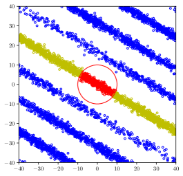
Figure 2: An illustration of Algorithm 1. Red: points inside a small ball; Yellow: the central stripe (${\mathbf{x}_{i}=\mathbf{y}_{i}}$).

The truncation radius.

In spite of its seeming simplicity, the behavior of Algorithm 1 depends drastically on the truncation radius $R$. Its choice should balance between two opposing effects. On the one hand, the algorithm uses effectively ${\mathbb{E}|\mathcal{K}|=n\cdot p_{\mathrm{Ball}}}$ measurements for estimation (where ${p_{\mathrm{Ball}}:=\Pr(\mathbf{X}\in\mathcal{B}(\bm{0},R)})$, so $R$ cannot be too small; on the other hand, we need to take only (or mostly) points from the central stripe, so $R$ cannot be too large. Let us start with an observation: when $R/\sqrt{k}<1$, $p_{\mathrm{Ball}}$ is exponentially small in $k$, so the algorithm requires $n\gtrsim 1/p_{\mathrm{Ball}}=\exp(\Omega(k))$ measurements. Consequently, to (potentially) overcome the curse of dimensionality one must set ${R/\sqrt{k}>1}$. In that case, $p_{\mathrm{Ball}}\approx 1\wedge(\sqrt{R/\nu})$ (Lemma 2), so that for a large spike, $\nu=\omega(R)$, $n\gtrsim\sqrt{\nu/R}$; therefore, we shall henceforth restrict our attention to $\nu=\mathrm{poly}(k)$. As we have said, $R$ cannot be chosen too large, and in general there is a rather delicate tradeoff between the parameters $\Delta,R,\nu$ and the direction $\mathbf{u}\in\mathbb{S}^{k-1}$ itself. Our main result, Theorem 1, says, roughly, the following: there is a choice $R=\Theta(\sqrt{k})$ such that for most directions, if $\Delta\gtrsim\sqrt{\log k}$ and $\nu=\mathrm{poly}(k)$, then Algorithm 1 estimates $\mathbf{u}$ with small error from only $n=\mathrm{poly}(k)$ measurements.

On estimating $\nu$.

In this paper, we restrict our attention to estimating only the direction $\mathbf{u}\in\mathbb{S}^{k-1}$ (and not $\nu$). We mention two potential strategies for estimating $\nu$, not pursued here further due to space constraints:

• [Palombi et al., 2012] studies covariance estimation from spherically-truncated Gaussian measurements. Relying on Proposition 1, they prove that the mapping $\bm{\lambda}\mapsto\bm{\mu}$ between the true and truncated eigenvalues is invertible, and propose a fixed point iteration to recover $\bm{\lambda}$ from $\bm{\mu}$ (given exactly, without noise). Our proposed algorithm computes an estimate of $\bm{\Sigma}_{\mathrm{Ball}}$; computing error bounds for the method of [Palombi et al., 2012], applied to $\widehat{{\bf{\Sigma}}}$, is potentially challenging, especially in the regime where $\nu\gg R^{2}=\Theta(k)$, where the mapping $\bm{\lambda}\mapsto\bm{\mu}$ is necessarily badly conditioned.

• Since only one eigenvalue of ${\bf{\Sigma}}$ is unknown, a more natural approach is to invert (numerically) the mapping $\nu\mapsto p_{\mathrm{Ball}}(\nu)=\Pr(\mathbf{X}\in\mathcal{B}(\bm{0},R))$, which is strictly decreasing.

2.1 Main results

The following is our main result. It shows that for most directions $\mathbf{u}\in\mathbb{S}^{k-1}$, the error attained by Algorithm 1 can be made quite small, with $n$ reasonably controlled, and assuming only $\Delta\gtrsim\sqrt{\log k}$. To make the presentation lighter, we focus exclusively on the regime where the spike is not small, $\nu=\Omega(1)$ (which is also practically more interesting). Below, $\widehat{\mathbf{u}}$ denotes the largest eigenvector of $\widehat{{\bf{\Sigma}}}$, with the sign ambiguity resolved by assuming that $\langle\mathbf{u},\widehat{\mathbf{u}}\rangle\geq 0$.

Theorem 1

Fix a constant $M>12$, and set $R=\Theta(\sqrt{k})$ as in (11). There is a universal constant $C_{*}$ and a set $\mathcal{U}_{M}\subseteq\mathbb{S}^{k-1}$ with

$$\Pr_{\mathbf{u}\sim\mathrm{Unif}(\mathbb{S}^{k-1})}(\mathbf{u}\in\mathcal{U}_{M})=1-O_{M}(k^{-10}),$$

such that whenever $\Delta\geq C_{*}(M\sqrt{\log k}\vee\nu^{\frac{1}{2(k-1)}})$ and $\mathbf{u}\in\mathcal{U}_{M}$, the following error bounds hold (depending on the magnitude of $\nu$), with probability $1-O(k^{-10})$:

1. Assume that $1\leq\nu\leq k$ and $n\gtrsim\log k$. Then

   $$\|\mathbf{u}-\widehat{\mathbf{u}}\|\lesssim\frac{1}{\sqrt{\nu}}\left(\frac{k}{n}\vee\sqrt{\frac{k}{n}}\right)+\nu^{-1}k^{-M^{2}+12}\,.$$ (8)

2. Assume that $k\leq\nu\lesssim k^{2M^{2}-21}$. Then

   $$\|\mathbf{u}-\widehat{\mathbf{u}}\|\lesssim\frac{\sqrt{\nu}}{n}+\sqrt{\frac{1}{n}\sqrt{\frac{\nu}{k}}}+\nu^{1/2}k^{-M^{2}+10.5}\,.$$ (9)

Discussion.

Let us start with the small-spike regime, $1\leq\nu\leq k$. The first term in Eq. (8) is, up to prefactors, the error rate for PCA without modulo-folding, see e.g. [Wainwright, 2019, Chapter 8]; in particular, when $k=O(n)$, it matches the minimax lower bound Eq. (4). The second term corresponds to error incurred by erroneously taking “bad” points $\mathbf{y}_{i}$, that do not belong on the central stripe. By taking $\Delta\gtrsim\sqrt{\log k}$ large enough, this term can be made to decay arbitrarily (polynomially) fast as $k\to\infty$. We note that in this regime, the consequences of Theorem 1 are, in fact, rather unsurprising: if $\mathbf{u}\sim\mathrm{Unif}(\mathbb{S}^{k-1})$, then with high probability, ${\|\mathbf{u}\|_{\infty}\lesssim\sqrt{\log k/k}}$. Since $\Delta\gtrsim\sqrt{\log k}$, the cube $[-\frac{1}{2}\Delta,\frac{1}{2}\Delta)^{k}$ contains a segment $\{t\mathbf{u}\,:\,t\in[-L,L]\}$ of length $2L\gtrsim\Delta/\|\mathbf{u}\|_{\infty}\gtrsim\sqrt{k}$; consequently, a large fraction of $\mathbf{x}_{1},\ldots,\mathbf{x}_{n}$ are actually themselves already inside the cube, since the “typical length” of the projection along $\mathbf{u}$, $|\langle\mathbf{u},\mathbf{X}\rangle|$, is $\lesssim\sqrt{\nu}$ (the standard deviation).

The “interesting” regime is $\nu\gg k$. Note that unlike in the small-spike regime, here the error, Eq. (9), increases as $\nu$ grows. Moreover, the magnitude of $\nu$ has to be constrained by $\Delta$: $\nu\lesssim k^{2M^{2}-21}$ (the constant $21$ is itself not particularly important, and can be improved). Thus, to retain the scaling $\Delta\sim\sqrt{\log k}$, $\nu$ has to grow at most polynomially with $k$; in that case, note that the term $\nu^{1/(2(k-1))}$ in the bound for $\Delta$ is always negligible. Furthermore, note that $n$ has to scale at least as $n\gtrsim\sqrt{\nu}$, which anyhow precludes the practically of the algorithm when $\nu$ is super-polynomial, regardless of the third term.

Let us try to get some intuition for the particular form of the bounds (8), (9), by considering a simplified setting, where one had direct access to all the measurements $\mathbf{x}_{i}$ that lie inside the ball $\mathcal{B}(\bm{0},R)$, and used them to perform PCA. There are roughly (Lemmas 1, 2)

$$\tilde{n}\approx p_{\mathrm{Ball}}n\approx(1\wedge\sqrt{k/\nu})n$$

such measurements. By Proposition 1, the population covariance $\bm{\Sigma}_{\mathrm{Ball}}$ is spiked, and one can show (Lemma 7) that the effective spike is

$$\tilde{\nu}\approx k\wedge\nu\,.$$

(Note that $\mathbf{X}_{\mathrm{Ball}}$ lies inside $\mathcal{B}(\bm{0},R)$, and consequently $\lambda_{1}(\bm{\Sigma}_{\mathrm{Ball}})\leq R^{2}=\Theta(k)$). In particular, note that when $\nu=\omega(k)$, $\tilde{n}$ decreases with $\nu$ but $\tilde{\nu}$ cannot grow further to compensate for this; this is the reason why the error in Eq. (9) degrades with $\nu$. Now, assuming that $\tilde{n}$ is large enough (this point is a little subtle, since we let $\tilde{\nu}$ grow as well), the error is bounded like

$$\|\mathbf{u}-\widehat{\mathbf{u}}\|\lesssim\frac{1}{\sqrt{\tilde{\nu}}}\left(\frac{k}{\tilde{n}}\vee\sqrt{\frac{k}{\tilde{n}}}\right)\,,$$

using “standard” bounds for PCA (e.g. [Wainwright, 2019, Chapter 8]). Plugging in the above estimates for $\tilde{n},\tilde{\nu}$ recovers the first terms in Eqs. (8), (9). The challenging part of the analysis (and our main technical contribution) is to control the last term: namely, show that for most directions $\mathbf{u}$, when $\Delta\gtrsim\sqrt{\log k}$, the contribution of the erroneously picked (“bad”) points is indeed very small with high probability.

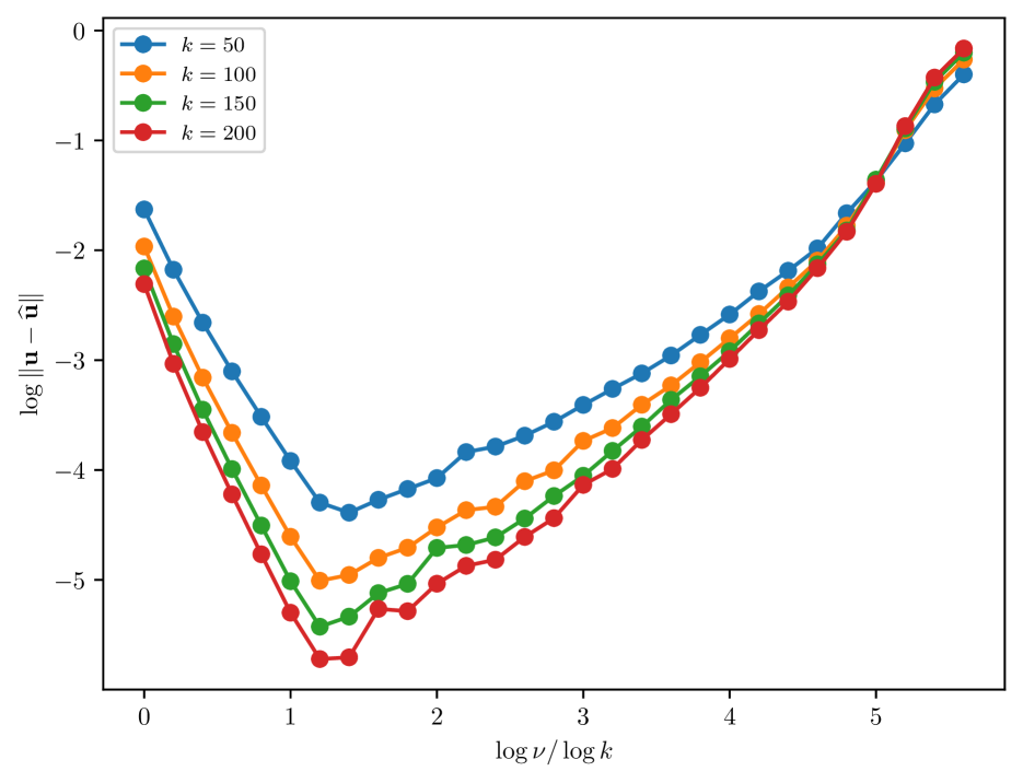
(a) The estimation error, ${\|\mathbf{u}-\widehat{\mathbf{u}}\|}$, as $\nu$ changes.

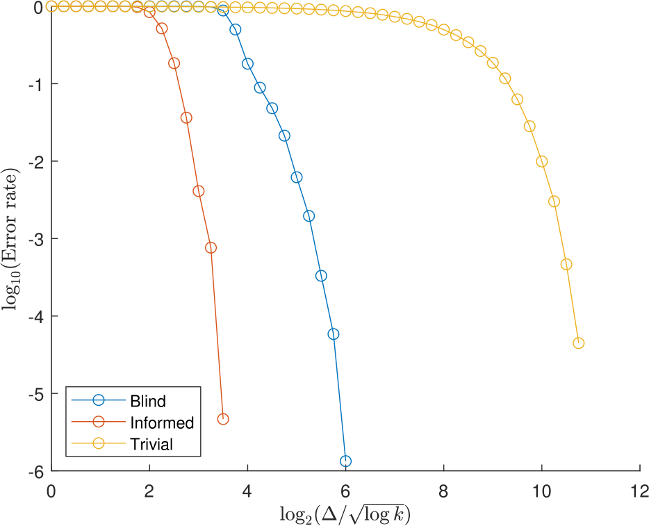
(b) Performance of the informed vs. blind integer forcing decoder, as $\Delta/\sqrt{\log k}$ changes.

Figure 3: Numerical results

Experiments.

We demonstrate the validity and relevance of our results through numerical experiments:

• In Figure 3(a) we study the behavior of the error, ${\|\mathbf{u}-\widehat{\mathbf{u}}\|}$, as the spike magnitude $\nu$ changes. For several values, $k=50,100,150,200$, we have set $\Delta=16\sqrt{\log k}$, $n=k^{2}$ and varied $\nu=k^{\alpha}$ for an exponent $\alpha\in[0,5.6]$; each point on the graph is the average error across $T=2400$ repetition. We observe that as $k$ increases, scaling $\Delta\propto\sqrt{\log k}$ indeed suffices for estimation. Moreover, we see that for small spikes, $\alpha<1$, the error decreases as $\alpha$ increases, whereas when $\alpha>1$ the error increases; this is consistent with Theorem 1.

• In Figure 3(b) we apply our algorithm as an intermediate step for blind unwrapping. We set $k=150$, $n=k^{2}\approx 2\cdot 10^{4}$, $\nu=k^{3}\approx 3\cdot 10^{6}$ and vary $\Delta=2^{\delta}\sqrt{\log k}$. At every working point, we compute the error rate, namely the fraction of erroneously recovered samples $\widehat{p}_{e}=\frac{1}{n}\sum_{i=1}^{n}\mathds{1}_{\mathbf{x}_{i}\neq\widehat{\mathbf{x}}_{i}}$, of the informed IF decoder (Eq. (6)), the blind IF decoder (computed from ${\widehat{{\bf{\Sigma}}}=\nu\widehat{\mathbf{u}}\widehat{\mathbf{u}}+\mathbf{I}}$), and the trivial decoder $\widehat{\mathbf{X}}=\mathbf{Y}$. For each method, $\delta$ is increased in jumps of $0.25$, until the point where $p_{e}\leq 10^{-4}$; each point on the graph is the average of $T=200$ repetitions (so, overall, $nT\approx 10^{6}$ single recovery trials). We see, for this particular setup, a gap of around $\delta=2$ bits between the the informed and blind decoders, and of about $\delta=5$ bits between the blind and trivial decoders. To put things in context, a hypothetical quantization scheme based around modulo-folding and the blind decoder could save up to $5$ bits per coordinate (so $5k=750$ bits overall) compared to the uniform quantizer (both designed so that the probability of a saturation is $\leq 10^{-4}$).

By Theorem 1, when $\nu=\mathrm{poly}(k)$, the condition $\Delta\gtrsim\sqrt{\log k}$ ensure that one can estimate most directions $\mathbf{u}\in\mathbb{S}^{k-1}$ with $n=\mathrm{poly}(k)$ measurements. Recall that the present problem was motivated by the modulo-unfolding problem (which is a harder problem). It turns out that for the latter, the condition $\Delta\gtrsim\sqrt{\log k}$ is actually necessary. Thus, if one’s goal is to solve the unwrapping problem (e.g. for implementing modulo-ADCs), and to that end estimates the covariance as an intermediate step, then our algorithm succeeds with essentially the smallest allowable dynamic range. We show the following (see Appendix B for the proof):

Proposition 2

Suppose that there exists $\widehat{\mathbf{X}}=\widehat{\mathbf{X}}(\mathbf{Y})$, with $\Pr(\mathbf{X}=\widehat{\mathbf{X}})\geq 0.1$. Then ${\Delta\gtrsim(\sqrt{\log k}\vee\nu^{\frac{1}{2k}})}$.

We remark in passing that, once we have obtained an estimate for $\mathbf{u}$, and consequently for ${\bf{\Sigma}}$, using Algorithm 1, we may use it to unwrap the measurements $\mathbf{x}_{1},\ldots,\mathbf{x}_{n}$ (using, e.g., the IF decoder). Having unwrapped the samples, we can use standard methods (e.g., PCA) to get an improved estimate of $\mathbf{u}$. We do not pursue this option here for two reasons: 1) The performance of such an algorithm depends on the unwrapping error probability, which is difficult to analyze. In particular, unwrapping errors could have a disastrous effect on the estimation error; 2) Our primary motivation for estimating $\mathbf{u}$ in the first place was to perform unwrapping. To that end, once we obtain an estimate of $\mathbf{u}$ with accuracy sufficient for unwrapping, further improvements are of limited interest.

3 Analysis

In this section, we give a proof outline for our main result, Theorem 1. In the interest of space, the proofs of most technical lemmas are relegated to the Appendix.

For $\delta\in(0,1)$, set

$$\begin{split}z_{2}(\delta)&:=\left(k+2\sqrt{k\log(1/\delta)}+2\log(1/\delta)\right)^{1/2}\,,\quad\\ z_{\infty}(\delta)&:=\sqrt{2\log k}+\sqrt{2\log(2/\delta)}\,,\end{split}$$ (10)

so that for $\mathbf{Z}\sim\mathcal{N}(\bm{0},\bm{I}_{k})$ (see Appendix H, Lemma 17),

$$\begin{split}&\Pr(\|\mathbf{Z}\|\geq z_{2}(\delta))\leq\delta,\quad\Pr(\|\mathbf{Z}\|_{\infty}\geq z_{\infty}(\delta))\leq\delta\,.\end{split}$$

Going forward, we fix a truncation radius:

$$R=2\sqrt{k}+z_{2}(0.1)=\Theta(\sqrt{k})\,.$$ (11)

This particular choice is rather arbitrary. One could carry out the analysis with any $R=C\sqrt{k}$ for $C>1$; this would only change the constants in the bounds.

3.1 High level view

Divide the pairs $\{(\mathbf{x}_{i},\mathbf{y}_{i})\}_{i\in[n]}$ into groups. Denote by

$$\mathcal{K}=\{i\in[n]\,:\,\mathbf{y}_{i}\in\mathcal{B}(\bm{0},R)\}\,,$$

$$\mathcal{K}_{\mathrm{Ball}}=\{i\in[n]\,:\,\mathbf{x}_{i}\in\mathcal{B}(\bm{0},R)\}\,,$$

respectively the points that were picked by Algorithm 1, and those for which $\mathbf{x}_{i}\in\mathcal{B}(\bm{0},R)$. Note that, conditioned on $i\in\mathcal{K}_{\mathrm{Ball}}$, $\mathbf{x}_{i}\overset{d}{=}\mathbf{X}_{\mathrm{Ball}}$; hence $\{\mathbf{x}_{i}\}_{i\in\mathcal{K}_{\mathrm{Ball}}}$ is an i.i.d. sample from $\mathbf{X}_{\mathrm{Ball}}$. Observe also that $\mathcal{K}_{\mathrm{Ball}}\subseteq\mathcal{K}$, since $\|\mathbf{X}\bmod\Delta\|\leq\|\mathbf{X}\|$. We denote by $\mathcal{K}_{\mathrm{Good}}\subseteq\mathcal{K}_{\mathrm{Ball}}$ the subset of measurements for which $\mathbf{x}_{i}=\mathbf{y}_{i}$, in other words, such that $\mathbf{x}_{i}\in[-\frac{1}{2}\Delta,\frac{1}{2}\Delta)^{k}$ to begin with. The measurements in $\mathcal{K}_{\mathrm{Bad}}=\mathcal{K}\setminus\mathcal{K}_{\mathrm{Good}}$, will be called bad. We have

$$\mathcal{K}_{\mathrm{Good}}\subseteq\mathcal{K}_{\mathrm{Ball}}\subseteq\mathcal{K}=\mathcal{K}_{\mathrm{Good}}\sqcup\mathcal{K}_{\mathrm{Bad}}\subseteq[n]\,.$$

Now, the sample covariance,

$$\widehat{{\bf{\Sigma}}}_{\mathbf{X}}:=\frac{1}{|\mathcal{K}_{\mathrm{Ball}}|}\sum_{i\in\mathcal{K}_{\mathrm{Ball}}}\mathbf{x}_{i}\mathbf{x}_{i}^{\top}$$ (12)

is a consistent (as $|\mathcal{K}_{\mathrm{Ball}}|\to\infty$) estimator for $\bm{\Sigma}_{\mathrm{Ball}}$, whose largest eigenvector is $\mathbf{u}$ (Proposition 1). Consequently, PCA yields a consistent estimator for the unknown direction. Alas, the set $\mathcal{K}_{\mathrm{Ball}}$ is not directly observable, so the algorithm uses $\mathcal{K}\supseteq\mathcal{K}_{\mathrm{Ball}}$ instead:

$$\widehat{{\bf{\Sigma}}}=\frac{1}{|\mathcal{K}_{\mathrm{Ball}}|}\sum_{i\in\mathcal{K}}\mathbf{y}_{i}\mathbf{y}_{i}^{\top}\,.$$ (13)

This injects additional error into the covariance estimation process, in two ways. First, the covariance is computed using the $\mathbf{y}_{i}$-s instead of the $\mathbf{x}_{i}$-s (the latter are unknown); we have $\mathbf{y}_{i}=\mathbf{x}_{i}$ only for $i\in\mathcal{K}_{\mathrm{Good}}$, which may be a strict subset of $\mathcal{K}$. Second, we use additional samples, on top of $\mathcal{K}_{\mathrm{Ball}}$: the points in $\mathcal{K}\setminus\mathcal{K}_{\mathrm{Ball}}$ necessarily come from the wrong distribution. Set

$$\begin{split}\varepsilon_{\mathrm{CovEst}}&:=\|\widehat{{\bf{\Sigma}}}_{\mathbf{X}}-\bm{\Sigma}_{\mathrm{Ball}}\|\,,\quad\varepsilon_{\mathrm{Pick}}:=\|\widehat{{\bf{\Sigma}}}_{\mathbf{X}}-\widehat{{\bf{\Sigma}}}\|\,,\end{split}$$

so that $\|\widehat{{\bf{\Sigma}}}-\bm{\Sigma}_{\mathrm{Ball}}\|\leq\varepsilon_{\mathrm{CovEst}}+\varepsilon_{\mathrm{Pick}}$. A bound on this operator norm yields, by standard eigenvector perturbation results, a bound on $\|\mathbf{u}-\widehat{\mathbf{u}}\|$. Note: $\varepsilon_{\mathrm{CovEst}}$ is simply the statistical estimation error in estimating $\bm{\Sigma}_{\mathrm{Ball}}=\mathrm{Cov}(\mathbf{X}_{\mathrm{Ball}})$ from $|\mathcal{K}_{\mathrm{Ball}}|$ i.i.d. measurements; the other term, $\varepsilon_{\mathrm{Pick}}$, is the error induced through picking erroneous measurements. We shall bound each error term separately.

3.2 The covariance estimation error

We start with $\varepsilon_{\mathrm{CovEst}}$; the argument is quite standard. First, we show that with high probability, $|\mathcal{K}_{\mathrm{Ball}}|$ is reasonably large. Denote

$$p_{\mathrm{Ball}}=p_{\mathrm{Ball}}(\nu;R)=\Pr\left(\mathbf{X}\in\mathcal{B}(\bm{0},R)\right)\,,$$ (14)

so that $|\mathcal{K}_{\mathrm{Ball}}|\sim\mathrm{Binomial}\left(p_{\mathrm{Ball}},n\right)$. Controlling $|\mathcal{K}_{\mathrm{Ball}}|$ is straightforward using, e.g., Chernoff’s inequality (Appendix H, Lemma 19):

Lemma 1

For any $\mathbf{u}\in\mathbb{S}^{k-1}$, for universal $c_{1},c_{2}>0$,

$$\Pr\left(|\mathcal{K}_{\mathrm{Ball}}|\leq c_{1}p_{\mathrm{Ball}}n\,\big{|}\,\mathbf{u}\right)\leq 2e^{-c_{2}p_{\mathrm{Ball}}n}\,.$$

Next is an (tight, for large $\nu$) estimate for $p_{\mathrm{Ball}}$; the (short) proof is relegated to Appendix G.1:

Lemma 2

$$0.9\,\mathrm{erf}\left(\sqrt{\frac{2k}{\nu}}\right)\leq p_{\mathrm{Ball}}\leq\mathrm{erf}\left(\sqrt{\frac{2k+z_{2}(0.1)/2}{1+\nu}}\right)\,,$$

where, recall, the error function is defined by

$$\mathrm{erf}(x)=\frac{2}{\sqrt{\pi}}\int_{0}^{x}e^{-t^{2}}dt=\Pr(|\xi|\leq\sqrt{2}x)\,.$$ (15)

Note that Lemma 2 implies that $p_{\mathrm{Ball}}=\Theta(1)$ when $\nu=O(k)$, whereas $p_{\mathrm{Ball}}=\Theta(\sqrt{k/\nu})$ when $\nu=\omega(k)$; in other words, $p_{\mathrm{Ball}}=\Theta(1\wedge\sqrt{k/\nu})$.

Error bounds for covariance estimation rely on the concentration properties of the data. Thus, we need to show that $\mathbf{X}_{\mathrm{Ball}}$ “inherits” the favorable properties of the underlying Gaussian vector $\mathbf{X}$. We start with a general Lemma, whose proof appears in Appendix G.2:

Lemma 3

For every convex function $g:\mathbb{R}^{k}\to\mathbb{R}$,

$$\mathbb{E}\left[g(\mathbf{X}_{\mathrm{Ball}})\right]\leq\mathbb{E}\left[g(\mathbf{X})\right]\,.$$

The proof of Lemma 3 relies on the Gaussian correlation inequality. As an important corollary, it allows us to control the sub-Gaussian and sub-exponential norms of $\mathbf{X}_{\mathrm{Ball}}$; see Appendix C, Lemma 9.

Recall that by Proposition 1, $\bm{\Sigma}_{\mathrm{Ball}}$ is a spiked covariance matrix with largest eigenvector $\mathbf{u}$:

$$\lambda_{1}(\bm{\Sigma}_{\mathrm{Ball}})>\lambda_{2}(\bm{\Sigma}_{\mathrm{Ball}})=\ldots=\lambda_{k}(\bm{\Sigma}_{\mathrm{Ball}})\,,$$

so that applying Lemma 3 (with $g(\mathbf{X})=\langle\mathbf{u}_{i},\mathbf{X}\rangle^{2}$),

$$\lambda_{1}(\bm{\Sigma}_{\mathrm{Ball}})\leq R^{2}\wedge(1+\nu),\quad\lambda_{2}(\bm{\Sigma}_{\mathrm{Ball}})\leq 1\,.$$

The rest of the analysis proceeds along rather standard lines, as in e.g. [Wainwright, 2019, Section 8.2.2]; the full details are given in Appendix C. We prove:

Lemma 4

Suppose that $p_{\mathrm{Ball}}n\gtrsim\log k$. Then, with probability $1-O(k^{-10})$,

$$\begin{split}\varepsilon_{\mathrm{CovEst}}&\lesssim(k\wedge(1+\nu))\sqrt{\frac{\log k}{p_{\mathrm{Ball}}n}}\\ &+\sqrt{(k\wedge(1+\nu)}\left({\frac{k}{p_{\mathrm{Ball}}n}}\vee\sqrt{\frac{k}{p_{\mathrm{Ball}}n}}\right)\,.\end{split}$$

3.3 The sample picking error

Decompose

$$\sum_{i\in\mathcal{K}}\mathbf{y}_{i}\mathbf{y}_{i}^{\top}=\sum_{i\in\mathcal{K}_{\mathrm{Good}}}\mathbf{x}_{i}\mathbf{x}_{i}^{\top}+\sum_{i\in\mathcal{K}_{\mathrm{Bad}}}\mathbf{y}_{i}\mathbf{y}_{i}^{\top}\,,$$

so that

$$\begin{split}\varepsilon_{\mathrm{Pick}}&=\frac{1}{|\mathcal{K}_{\mathrm{Ball}}|}\cdot\left\|\sum_{i\in\mathcal{K}_{\mathrm{Bad}}}\mathbf{y}_{i}\mathbf{y}_{i}^{\top}-\sum_{i\in\mathcal{K}_{\mathrm{Ball}}\setminus\mathcal{K}_{\mathrm{Good}}}\mathbf{x}_{i}\mathbf{x}_{i}^{\top}\right\|\\ &\leq\frac{2|\mathcal{K}_{\mathrm{Bad}}|\cdot R^{2}}{|\mathcal{K}_{\mathrm{Ball}}|}\lesssim k\cdot\frac{|\mathcal{K}_{\mathrm{Bad}}|}{|\mathcal{K}_{\mathrm{Ball}}|}\,.\end{split}$$ (16)

Above, we used: $\|\mathbf{x}_{i}\|\leq R$ for $i\in\mathcal{K}_{\mathrm{Ball}}$; $\|\mathbf{y}_{i}\|\leq R$ for $i\in\mathcal{K}$; and $\left|\mathcal{K}_{\mathrm{Ball}}\setminus\mathcal{K}_{\mathrm{Good}}\right|\leq\left|\mathcal{K}\setminus\mathcal{K}_{\mathrm{Good}}\right|\leq\left|\mathcal{K}_{\mathrm{Bad}}\right|$.

The next Lemma is one of our main technical results. It states that for most directions $\mathbf{u}\in\mathbb{S}^{k-1}$, the probabiliy that a pair $(\mathbf{X},\mathbf{Y})$ is bad, meaning that $\mathbf{Y}\in\mathcal{B}(\bm{0},R)$ but $\mathbf{X}\neq\mathbf{Y}$, is overwhelmingly small provided that $\Delta\gtrsim\sqrt{\log k}\vee\nu^{\frac{1}{2(k-1)}}$:

Lemma 5

Fix a constant $M\geq 1$. There is a universal $C_{*}>0$ and a subset $\mathcal{U}_{M}\subseteq\mathbb{S}^{k-1}$ with

$$\Pr_{\mathbf{u}\sim\mathrm{Unif}(\mathbb{S}^{k-1})}\left(\mathbf{u}\in\mathcal{U}_{M}\right)=1-O_{M}(k^{-10})\,,$$

such that if $\Delta\geq C_{*}(M\sqrt{\log k}\vee\nu^{\frac{1}{2(k-1)}})$, then for all $\mathbf{u}\in\mathcal{U}_{M}$,

$$\Pr\left((\mathbf{X},\mathbf{Y})\textnormal{ is bad }\,\big{|}\,\mathbf{u}\right)\leq k^{-M^{2}}\,.$$

The proof appears in Appendix D. The key idea is to reduce the problem into a question in geometric probability: whether a randomly rotated line segment is far away from all non-zero lattice points.

Lemma 5 readily gives the following bound; the details are given in Appendix G.3:

Lemma 6

Assume the setup of Lemma 5, with ${M>\sqrt{12}}$, $\mathbf{u}\in\mathcal{U}_{M}$, $\Delta\geq C_{*}(M\sqrt{\log k}\vee\nu^{\frac{1}{2(k-1)}})$. Suppose that $p_{\mathrm{Ball}}n\gtrsim\log k$. With probability $1-O(k^{-10})$:

$$\varepsilon_{\mathrm{Pick}}\lesssim\frac{k^{-M^{2}+12}}{p_{\mathrm{Ball}}}\,.$$

3.4 Concluding the analysis

So far, we have shown that $\|\widehat{{\bf{\Sigma}}}-\bm{\Sigma}_{\mathrm{Ball}}\|$ is small with high probability. To deduce that their largest eigenvectors are close as well (using eigenvector perturbation results), we first need to show that the spectral gap of $\bm{\Sigma}_{\mathrm{Ball}}$ is large. We prove the following in Appendix E:

Lemma 7

There are universal $C_{1},C_{2}$ such that for $\nu\geq e^{-C_{1}k}$,

$$\lambda_{1}(\bm{\Sigma}_{\mathrm{Ball}})\geq 1+C_{2}(k\wedge\nu)\,.$$

Consequently, $\lambda_{1}(\bm{\Sigma}_{\mathrm{Ball}})-\lambda_{2}(\bm{\Sigma}_{\mathrm{Ball}})\gtrsim(k\wedge\nu)$.

The proof of Theorem 1 follows by combining our bounds thus far. The details appear in Appendix F.

Acknowledgements

This work was supported in part by ISF under Grant 1791/17 and in part by the GENESIS Consortium via the Israel Ministry of Economy and Industry. The work of Elad Romanov was supported in part by an Einstein-Kaye fellowship from the Hebrew University of Jerusalem.

Appendix A Proof of Proposition 1, Item 1

Decompose $\mathbf{X}$ along the principal components:

$$\mathbf{X}=\sum_{i=1}^{k}\sqrt{\lambda_{i}}g_{i}\mathbf{u}_{i}\,,$$

where $g_{1},\ldots,g_{k}\overset{i.i.d.}{\sim}\mathcal{N}(0,1)$. Then,

$$\bm{\Sigma}_{\mathrm{Ball}} =\mathbb{E}\left[\mathbf{X}\mathbf{X}^{\top}\,\big{|}\,\|\mathbf{X}\|^{2}\leq R^{2}\right]=\sum_{i,j=1}^{k}\mathbb{E}\left[\sqrt{\lambda_{i}\lambda_{j}}g_{i}g_{j}\mathbf{u}_{i}\mathbf{u}_{j}^{\top}\,\Big{|}\,\sum_{i=1}^{k}\lambda_{i}g_{i}^{2}\leq R^{2}\right]\,.$$

Now, observe that the cross terms, $i\neq j$, are zero, since conditioning onto the ball preserves the symmetry $(g_{i},g_{j})\mapsto(-g_{i},g_{j})$. Thus,

$$\bm{\Sigma}_{\mathrm{Ball}}=\sum_{i=1}^{k}\mathbb{E}\left[\lambda_{i}g_{i}^{2}\mathbf{u}_{i}\mathbf{u}_{i}^{\top}\,\Big{|}\,\sum_{i=1}^{k}\lambda_{i}g_{i}^{2}\leq R^{2}\right]=:\sum_{i=1}^{k}\mu_{i}\mathbf{u}_{i}\mathbf{u}_{i}^{\top}\,,$$

and so the claim is proved.

Appendix B Proof of Proposition 2

For brevity, define

$$p(\nu;\mathbf{u})=\Pr_{\mathbf{X}\sim\mathcal{N}(\bm{0},\nu\mathbf{u}\mathbf{u}^{\top}+\bm{I})}\left(\mathbf{X}=\widehat{\mathbf{X}}_{\mathrm{MAP}}\right)\,,$$ (17)

where $\mathbf{X}_{\mathrm{MAP}}$ is the MAP estimator of $\mathbf{X}$ from $\mathbf{Y}=[\mathbf{X}]\bmod\Delta$; in other words, $p(\nu;\mathbf{u})$ is the success probability of the MAP estimator at SNR $\nu$ with spike direction $\mathbf{u}$. Recalling that the MAP estimator is optimal in the sense of error probability, it is clear that to prove Proposition 2, it suffices to show that $p(\nu;\mathbf{u})\geq 0.1$ implies that $\Delta\gtrsim\nu^{1/2k}\vee\sqrt{\log k}$.

We start with a simple observation:

Lemma 8

The function $\nu\mapsto p(\nu;\mathbf{u})$ is decreasing.

Proof. For any $\nu\geq 0$, denote $\mathbf{X}_{\nu}\sim\mathcal{N}(\bm{0},\nu\mathbf{u}\mathbf{u}^{\top}+\bm{I})$ and $\mathbf{Y}_{\nu}=[\mathbf{X}_{\nu}]\bmod\Delta$, and let $g_{\nu}:[-\Delta/2,\Delta/2)^{k}\to\mathbb{R}^{k}$ be a deterministic function such that $g_{\nu}(\mathbf{Y}_{\nu})$ is the MAP estimator for $\mathbf{X}_{\nu}$. Fix any $\tau\geq 0$; we shall now construct a suboptimal estimator for $\mathbf{X}_{\nu}$ given $\mathbf{Y}_{\nu}$, based on $g_{\nu+\tau}(\cdot)$. The idea is simple: we generate known noise $\mathbf{N}\sim\mathcal{N}(\bm{0},\tau\mathbf{u}\mathbf{u}^{\top})$ and set $\mathbf{Y}^{\prime}=[\mathbf{Y}_{\nu}+\mathbf{N}]\bmod\Delta$, which also equals $\mathbf{Y}^{\prime}=[\mathbf{X}_{\nu}+\mathbf{N}]\bmod\Delta$. Note that $(\mathbf{X}_{\nu+\tau},\mathbf{Y}_{\nu+\tau})\overset{d}{=}(\mathbf{X}_{\nu}+\mathbf{N},\mathbf{Y}^{\prime})$. Considering the sub-optimal estimator $\widehat{\mathbf{X}}^{\prime}=g_{\nu+\tau}(\mathbf{Y}^{\prime})-\mathbf{N}$ for $\mathbf{X}_{\nu}$, we conclude,

$$p({\nu;\mathbf{u}})\geq\Pr(\mathbf{X}_{\nu}=\widehat{\mathbf{X}}^{\prime})=\Pr\left(\mathbf{X}_{\nu}=g_{\nu+\tau}(\mathbf{Y}^{\prime})-\mathbf{N}\right)=\Pr\left(\mathbf{X}_{\nu+\tau}=g_{\nu+\tau}(\mathbf{Y}_{\nu+\tau})\right)=p({\nu+\tau;\mathbf{u}})\,.$$

 

Let us start by showing $\Delta\gtrsim\sqrt{\log k}$. By Lemma 8, the assumptions of Proposition 2 imply that $p(0;\mathbf{u})\geq 0.1$. Now, it is easy to see that when $\nu=0$, $\widehat{\mathbf{X}}_{\mathrm{MAP}}=\mathbf{Y}$; in this case, the problem simply decouples across the different coordinates. Thus,

$$0.1\leq p(0;\mathbf{u})=\Pr(\mathbf{X}=\mathbf{Y})=\Pr\left(|X_{i}|\leq\Delta/2\,\textrm{ for all }1\leq i\leq k)\right)=\left\{\mathrm{erf}\left(\Delta/2^{3/2}\right)\right\}^{k}\,,$$

and therefore $\mathrm{erf}(\Delta/2^{3/2})\geq 1-ck^{-1}$ for some universal $c\geq 0$. Clearly, then, $\Delta=\omega(1)$ for large $k$, so by the standard estimate $1-\mathrm{erf}(x)\gtrsim e^{-x^{2}}/x$ (for large $x$), we get $e^{-c_{1}\Delta^{2}}/\Delta\lesssim 1/k$ hence $\Delta\gtrsim\sqrt{\log k}$.

It remains to show $\Delta\gtrsim\nu^{1/2k}$. To that end, we will use a simple geometric characterization of the MAP estimator, following [Romanov and Ordentlich, 2021]. Let

$$\mathcal{L}=\Delta{\bf{\Sigma}}^{-1/2}\mathbb{Z}^{k}=\left\{\Delta{\bf{\Sigma}}^{-1/2}\mathbf{t}\,:\,\mathbf{t}\in\mathbb{Z}^{k}\right\}$$

be the lattice generated by the matrix $\Delta{\bf{\Sigma}}^{-1/2}$, and denote by $V_{0}\subset\mathbb{R}^{k}$ the Voronoi cell of $\bm{0}\in\mathcal{L}$ (that is, all points $\mathbf{a}\in\mathbb{R}^{k}$ whose closest lattice point is $\bm{0}\in\mathcal{L}$). By [Romanov and Ordentlich, 2021, Section III, Eq. (38)], the success probability of the MAP estimator is

$$\Pr\left(\widehat{\mathbf{X}}^{\mathrm{MAP}}(\mathbf{Y})=\mathbf{X}\right)=\Pr_{\mathbf{Z}\sim\mathcal{N}(0,\mathbf{I}_{k})}\left(\mathbf{Z}\in V_{0}\right)\,.$$

Now, it is a well-known fact that $V_{0}$ is a convex symmetric set, with $\mathrm{vol}_{k}(V_{0})=|\Delta{\bf{\Sigma}}^{-1/2}|=\Delta^{k}/|{\bf{\Sigma}}|^{1/2}$. Let $r_{0}$ be the effective radius of $\mathcal{L}$, defined by

$$\mathrm{vol}_{k}(\mathcal{B}(\bm{0},r_{0}))=\mathrm{vol}_{k}(V_{0})\Longrightarrow r_{0}=\frac{\Delta}{|{\bf{\Sigma}}|^{\frac{1}{2k}}\mathcal{V}_{k}^{1/k}}\,,$$

($\mathcal{V}_{k}$ denotes the volume of the Euclidean unit ball). Recall that among all convex bodies with a given (finite) volume, a ball has the largest Gaussian measure. Thus,

$$0.1\leq\Pr_{\mathbf{Z}\sim\mathcal{N}(0,\mathbf{I}_{k})}\left(\mathbf{Z}\in V_{0}\right)\leq\Pr_{\mathbf{Z}\sim\mathcal{N}(0,\mathbf{I}_{k})}\left(\mathbf{Z}\in\mathcal{B}(\bm{0},r_{0})\right)=\Pr_{\mathbf{Z}\sim\mathcal{N}(0,\mathbf{I}_{k})}\left(\|\mathbf{Z}\|^{2}\leq r_{0}^{2}\right)\,.$$

Note that $\|\mathbf{Z}\|^{2}\sim\chi^{2}_{(k)}$, which concentrates around $k$ with “typical” deviations of order $O(\sqrt{k})$ (see, e.g., Lemma 17). This gives $r_{0}\gtrsim\sqrt{k}$, so

$$\Delta\gtrsim|{\bf{\Sigma}}|^{\frac{1}{2k}}\left(\mathcal{V}_{k}^{1/k}\sqrt{k}\right)=(1+\nu)^{1/2k}\left(\mathcal{V}_{k}^{1/k}\sqrt{k}\right)\gtrsim(1+\nu)^{1/2k}\,,$$

where the last inequality follows from Stirling’s approximation: $\mathcal{V}_{k}\overset{k\to\infty}{\approx}\frac{1}{\sqrt{k\pi}}\left(\frac{2\pi e}{k}\right)^{k/2}$, and therefore ${\mathcal{V}_{k}^{1/k}\sqrt{k}=\sqrt{2\pi e}+o(1)=\Theta(1)}$.

Appendix C Proof of Lemma 4

Decompose $\mathbf{X}_{\mathrm{Ball}}$ along the principal components:

$$\mathbf{X}_{\mathrm{Ball}}=w\mathbf{u}+\mathbf{p}\,,$$

where $w$ is the projection along $\mathbf{u}$ and $\mathbf{p}$ is the orthogonal complement. Note that, while $w$ and $\mathbf{p}$ are uncorrelated, they are not independent (as was the case without truncation, for a Gaussian vector) since we condition on $w^{2}+\|\mathbf{p}\|^{2}\leq R^{2}$. Also, recalling the “spiky” structure of $\bm{\Sigma}_{\mathrm{Ball}}$,

$$\mathbb{E}(w^{2})=\lambda_{1}(\bm{\Sigma}_{\mathrm{Ball}}),\quad\mathbb{E}[\mathbf{p}\mathbf{p}^{\top}]=\bm{\Sigma}_{\mathrm{Ball}}-\lambda_{1}(\bm{\Sigma}_{\mathrm{Ball}})\cdot\mathbf{u}\mathbf{u}^{\top}=\lambda_{2}(\bm{\Sigma}_{\mathrm{Ball}})\cdot(\bm{I}-\mathbf{u}\mathbf{u}^{\top})\,.$$ (18)

Condition on $N=|\mathcal{K}_{\mathrm{Ball}}|$, and denote for convenience $\mathcal{K}_{\mathrm{Ball}}=\{1,\ldots,N\}$, so that $\{\mathbf{x}_{i}\}_{i=1}^{N}$ are i.i.d. measurements from $\mathbf{X}_{\mathrm{Ball}}$. Write

$$\begin{split}\widehat{{\bf{\Sigma}}}_{\mathbf{X}}&=\frac{1}{N}\sum_{i=1}^{N}\left(w_{i}\mathbf{u}+\mathbf{p}_{i}\right)\left(w_{i}\mathbf{u}+\mathbf{p}_{i}\right)^{\top}\\ &=\left(\frac{1}{N}\sum_{i=1}^{N}w_{i}^{2}\right)\mathbf{u}\mathbf{u}^{\top}+\left(\frac{1}{N}\sum_{i=1}^{N}w_{i}\mathbf{p}_{i}\right)\mathbf{u}^{\top}+\left(\frac{1}{N}\left(\sum_{i=1}^{N}w_{i}\mathbf{p}_{i}\right)\mathbf{u}^{\top}\right)^{\top}+\frac{1}{N}\sum_{i=1}^{N}\mathbf{p}_{i}\mathbf{p}_{i}^{\top}\,,\end{split}$$ (19)

so that the error can be decomposed as $\left\|\widehat{{\bf{\Sigma}}}_{\mathbf{X}}-\bm{\Sigma}_{\mathrm{Ball}}\right\|\leq\varepsilon_{1}+2\varepsilon_{2}+\varepsilon_{3}$, with

$$\begin{split}\varepsilon_{1}&:=\left|\frac{1}{N}\sum_{i=1}^{N}w_{i}^{2}-\mathbb{E}[w^{2}]\right|\,,\\ \varepsilon_{2}&:=\left\|\frac{1}{N}\sum_{i=1}^{N}w_{i}\mathbf{p}_{i}\right\|\,,\\ \varepsilon_{3}&:=\left\|\frac{1}{N}\sum_{i=1}^{N}\mathbf{p}_{i}\mathbf{p}_{i}^{\top}-\mathbb{E}\left[\mathbf{p}\mathbf{p}^{\top}\right]\right\|\,.\end{split}$$ (20)

We first show that $\mathbf{X}_{\mathrm{Ball}}$ inherits the sub-Gaussian concentration properties of $\mathbf{X}$. We denote, respectively, the sub-Gaussian and sub-exponential norms by $\|\cdot\|_{\psi_{2}}$ and $\|\cdot\|_{\psi_{1}}$. For a quick reminder on these norm (and Orlicz norms in general), see Definition 1 and Lemma 20.

Lemma 9

We have

$$\|\mathbf{p}\|_{\psi_{2}}\lesssim 1\,,\quad\|w^{2}\|_{\psi_{1}}\lesssim k\wedge(1+\nu)\,.$$

and

$$\left\|w\mathbf{p}\right\|_{\psi_{1}}\lesssim\sqrt{k\wedge(1+\nu)}\,.$$

Proof. Let $\psi:[0,\infty)\to[0,\infty)$ be convex and increasing, and let $g:\mathbb{R}\to\mathbb{R}$ be such that $\mathbf{x}\mapsto|g(\mathbf{x})|$ is convex. Observe that $x\mapsto\psi(|g(x)|)$ is convex, and consequently, by Lemma 3, $\|g(\mathbf{X}_{\mathrm{Ball}})\|_{\psi}\leq\|g(\mathbf{X})\|_{\psi}$, where $\|\cdot\|_{\psi}$ is the Orlicz $\psi$-norm (see Definition 1). Consequently,

$$\|w^{2}\|_{\psi_{1}}\leq\|\langle\mathbf{u},\mathbf{X}\rangle^{2}\|_{\psi_{1}}\lesssim 1+\nu,\quad\|\mathbf{p}\|_{\psi_{2}}\leq\left\|(\mathbf{I}-\mathbf{u}\mathbf{u}^{\top})\mathbf{X}\right\|_{\psi_{2}}\lesssim 1\,.$$

Furthermore, using Lemma 20, Items 1 and 5,

$$\|w^{2}\|_{\psi_{1}}=\|w\|_{\psi_{2}}^{2}\lesssim\|w\|^{2}_{\infty}\leq R^{2}\lesssim k\,.$$

This proves the first two bound. As for the last one,

$$\|w\mathbf{p}\|_{\psi_{1}}=\sup_{\mathbf{v}\in\mathbb{S}^{k-1}}\|w\langle\mathbf{v},\mathbf{p}\rangle\|_{\psi_{1}}\overset{(\star)}{\leq}\|w\|_{\psi_{2}}\cdot\sup_{\mathbf{v}\in\mathbb{S}^{k-1}}\|\langle\mathbf{v},\mathbf{p}\rangle\|_{\psi_{2}}=\|w\|_{\psi_{2}}\|\mathbf{p}\|_{\psi_{2}}\overset{(\star\star)}{\lesssim}\sqrt{k\wedge(1+\nu)}\,,$$

where $(\star)$ follows from Lemma 20, Item 2, and $(\star\star)$ follows from Lemma 20, Item 1, and the first part of this proof.   

We now bound the errors $\varepsilon_{1},\varepsilon_{2},\varepsilon_{3}$, again conditioned on $N=|\mathcal{K}_{\mathrm{Ball}}|$:

Lemma 10

Assume that $N\gtrsim\log k$. Then, with probability $1-O(k^{-10})$,

$$\varepsilon_{1}\lesssim(k\wedge(1+\nu))\sqrt{\frac{\log k}{N}}\,.$$

Proof. By the centralization Lemma (Lemma 20, Item 3) and Lemma 9,

$$\left\|w_{i}^{2}-\mathbb{E}\left[w_{i}^{2}\right]\right\|_{\psi_{1}}\leq\|w_{i}^{2}\|_{\psi_{1}}\lesssim k\wedge(1+\nu)\,.$$

By Bernstein’s inequality (Lemma 21),

$$\Pr\left(\varepsilon_{1}\geq t\right)\leq 2\exp\left[-c_{1}N(\delta\wedge\delta^{2})\right],\quad\delta:=\frac{t}{k\wedge(1+\nu)}\,.$$

Set $t=\sqrt{\frac{{10}}{c_{1}}}(k\wedge(1+\nu))\sqrt{\frac{\log k}{N}}$. Then whenever $N\geq\frac{10}{c_{1}}\log k$, the probability is $\leq 2k^{-10}$.   

Lemma 11

With probability $1-2e^{-\Omega(k)}$,

$$\varepsilon_{2}\lesssim\sqrt{k\wedge(1+\nu)}\left(\frac{k}{N}\vee\sqrt{\frac{k}{N}}\right)\,.$$

Proof. Set $\mathbf{q}=\frac{1}{N}\sum_{i=1}^{N}w_{i}\mathbf{p}_{i}$, and observe that $\mathbb{E}[\mathbf{q}]=\bm{0}$, since $w_{i}$ and $\mathbf{p}_{i}$ are uncorrelated. We want to bound $\|\mathbf{q}\|$ with high probability; to that end, we use a standard $\varepsilon$-net argument, executed in detail for the sake of completeness. Using [Vershynin, 2018, Corollary 4.2.13], fix a $1/2$-net $\mathcal{N}$ of $\mathbb{S}^{k-1}$ of size $|\mathcal{N}|\leq 5^{k}$. Let $\tilde{\mathbf{v}}\in\mathcal{N}$ be a member of the net, such that $\left\|\frac{\mathbf{q}}{\|\mathbf{q}\|}-\tilde{\mathbf{v}}\right\|\leq 1/2$. Now,

$$\|\mathbf{q}\|=\left\langle\mathbf{q},\frac{\mathbf{q}}{\|\mathbf{q}\|}\right\rangle=\left\langle\mathbf{q},\frac{\mathbf{q}}{\|\mathbf{q}\|}-\tilde{\mathbf{v}}\right\rangle+\left\langle\mathbf{q},\tilde{\mathbf{v}}\right\rangle\leq\|\mathbf{q}\|\left\|\frac{\mathbf{q}}{\|\mathbf{q}\|}-\tilde{\mathbf{v}}\right\|+\langle\mathbf{q},\tilde{\mathbf{v}}\rangle\leq\frac{1}{2}\|\mathbf{q}\|+\langle\mathbf{q},\tilde{\mathbf{v}}\rangle\,,$$

which implies $\|\mathbf{q}\|\leq 2\langle\mathbf{q},\tilde{\mathbf{v}}\rangle$. Consequently, $\|\mathbf{q}\|\leq 2\max_{\mathbf{v}\in\mathcal{N}}\langle\mathbf{q},\mathbf{v}\rangle$, so it suffices to bound the latter. Recalling, by Lemma 9, that ${\|w_{i}\mathbf{p}_{i}\|_{\psi_{1}}\lesssim\sqrt{k\wedge(1+\nu)}}$, by Bernstein’s inequality and a union bound over the net,

$$\Pr\left(\max_{\mathbf{v}\in\mathcal{N}}\langle\mathbf{q},\mathbf{v}\rangle\geq t\right)\leq 2\cdot 5^{k}\cdot\exp\left[-c_{1}N(\delta\wedge\delta^{2})\right],\quad\delta:=\frac{t}{\sqrt{k\wedge(1+\nu)}}\,.$$

Set

$$t=\sqrt{k\wedge(1+\nu)}\left(\frac{10}{c_{1}}\frac{k}{N}\vee\sqrt{\frac{10}{c_{1}}\frac{k}{N}}\right)\,,$$

so that the probability is bounded by $2\cdot 5^{k}e^{-10k}=2e^{-\Omega(k)}$.   

Lemma 12

With probability $1-2e^{-\Omega(k)}$,

$$\varepsilon_{3}\lesssim\left(\frac{k}{N}\vee\sqrt{\frac{k}{N}}\right)\,.$$

Proof. By Lemma 9, the vectors $\mathbf{p}_{i}$ are $O(1)$-sub-Gaussian. The claim follows by Lemma 22, applied with $t\approx\sqrt{k}$, $\delta\approx\sqrt{\frac{k}{N}}$.   

Proof of Lemma 4.

The proof follows from Lemmas 10, 11 and 12, combined with $N\gtrsim p_{\mathrm{Ball}}n$ from Lemma 1.

Appendix D Proof of Lemma 5

The core of the argument is this: we reduce the question of whether ${\Pr((\mathbf{X},\mathbf{Y})\textnormal{ is bad}\,|\,\mathbf{u})}$ is large to a geometric question; specifically, whether a randomly rotated line segment is close to any non-zero lattice point. The details proceed as follow.

Recall: the pair $(\mathbf{X},\mathbf{Y})$ is bad when $\mathbf{Y}\in\mathcal{B}(\bm{0},R)$ but $\mathbf{X}\notin\mathcal{Q}_{\Delta}:=[-\frac{1}{2}\Delta,\frac{1}{2}\Delta)^{k}$. Our goal is to show that for most directions $\mathbf{u}\in\mathbb{S}^{k-1}$, the probability that $(\mathbf{X},\mathbf{Y})$ is bad is small, specifically,

$$\Pr\left((\mathbf{X},\mathbf{Y})\textnormal{ is bad}\,|\,\mathbf{u}\right)\leq k^{-M^{2}}\,.$$

We start by constraining ourselves to a set of “typical” vectors $\mathbf{X}$. As in Eq. (2), write, $\mathbf{X}=\sqrt{\nu}\xi\mathbf{u}+\mathbf{Z}$, for independent $\xi\sim\mathcal{N}(0,1)$, $\mathbf{Z}\sim\mathcal{N}(\bm{0},\mathbf{I})$. Let $\delta>0$ be a confidence parameter (we shall set $\delta=k^{-M^{2}}$ later), and consider the event

$$\mathcal{E}_{\mathbf{X}}=\left\{\|\mathbf{Z}\|_{2}\leq z_{2}(\delta/3),\,\|\mathbf{Z}\|_{\infty}\leq z_{\infty}(\delta/3),\,|\xi|\leq h(\delta/3)\right\}$$ (21)

where $h(\delta)=\sqrt{2\log(2/\delta)}$ is such that $\Pr(|\xi|\geq h(\delta))\leq\delta$, and $z_{2}(\delta),z_{\infty}(\delta)$ are as in Eq. (10). Clearly, $\Pr(\mathcal{E}_{\mathbf{X}})\leq\delta$.

Operating under $\mathcal{E}_{\mathbf{X}}$, let us bound the event $\{(\mathbf{X},\mathbf{Y})\textnormal{ is bad}\}$ by another, larger, event. To start, note that $\mathbf{X}\neq\mathbf{Y}$ implies that $\mathbf{X}=\mathbf{Y}+\Delta\mathbf{t}$ for some non-zero lattice vector $\mathbf{t}\in\mathbb{Z}^{k}\setminus\{\bm{0}\}$. Consequently, when $\mathbf{Y}\in\mathcal{B}(\bm{0},R)$, $\mathbf{X}\neq\mathbf{Y}$ implies that $\mathbf{X}\in\bigcup_{\mathbf{t}\in\mathbb{Z}^{k}\setminus\{\bm{0}\}}\mathcal{B}\left(\Delta\mathbf{t},R\right)$. Decomposing $\mathbf{X}$, this further implies that

$$\sqrt{\nu}\xi\mathbf{u}\in\bigcup_{\mathbf{t}\in\mathbb{Z}^{k}\setminus\{\bm{0}\}}\mathcal{B}\left(\Delta\mathbf{t},R+\|\mathbf{Z}\|\right)\,.$$ (22)

As for the condition $\mathbf{X}\notin\mathcal{Q}_{\Delta}$, equivalently $\|\mathbf{X}\|_{\infty}>\frac{1}{2}\Delta$, it follows from the triangle inequality that

$$\|\sqrt{\nu}\xi\mathbf{u}\|_{\infty}=|\sqrt{\nu}\xi|\|\mathbf{u}\|_{\infty}\geq\frac{1}{2}\Delta-\|\mathbf{Z}\|_{\infty}\,.$$ (23)

Let $\mathcal{U}_{1,M}\subseteq\mathbb{S}^{k-1}$ be the set of incoherent directions,

$$\mathcal{U}_{1,M}:=\left\{\mathbf{u}\in\mathbb{S}^{k-1}\,:\,\|\mathbf{u}\|_{\infty}\leq\frac{1}{C_{1}}\sqrt{\frac{\log k}{k}}\right\}\,,$$ (24)

with $C_{1}$ a universal constant such that $\Pr(\mathbf{u}\in\mathcal{U}_{1,M})=1-O(k^{-10})$ for $\mathbf{u}\sim\mathrm{Unif}(\mathbb{S}^{k-1})$ (see Lemma 18). Now, under $\mathcal{E}_{\mathbf{X}}$, and assuming that $\mathbf{u}\in\mathcal{U}_{1,M}$, Eqs. (22) and (23) imply that

$$\sqrt{\nu}\xi\mathbf{u}\in\bigcup_{\mathbf{t}\in\mathbb{Z}^{k}\setminus\{\bm{0}\}}\mathcal{B}\left(\Delta\mathbf{t},R_{\delta}\right),\quad|\sqrt{\nu}\xi|\geq C_{1}\Delta_{\delta}\sqrt{\frac{k}{\log k}}\,,$$ (25)

where we set

$$\Delta_{\delta}:=\frac{1}{2}\Delta-z_{\infty}(\delta/3),\quad R_{\delta}:=R+z_{2}(\delta/3)\,.$$ (26)

Henceforth, we shall assume $\Delta$ to be large enough so that $\Delta_{\delta}>0$. Consider the line segment, $L(\mathbf{u})\subset\mathbb{R}^{k}$,

$${L}(\mathbf{u})=\{s\mathbf{u}\quad:\quad A\leq s\leq B\}\,,\quad\textrm{where}\quad A:=C_{1}\Delta_{\delta}\sqrt{\frac{k}{\log k}},\,\,B:=\sqrt{\nu}h(\delta/3)=\sqrt{2\nu\log(6/\delta)}\,.$$ (27)

Observe that under $\mathcal{E}_{\mathbf{X}}$, the occurrence of the event in Eq. (25) implies, in particular, that

$$L(\mathbf{u})\cap\bigcup_{\mathbf{t}\in\mathbb{Z}^{k}\setminus\{\bm{0}\}}\mathcal{B}\left(\Delta\mathbf{t},R_{\delta}\right)\neq\emptyset\,.$$

Note that given $\mathbf{u}$, this is a deterministic geometric condition. Set

$$\mathcal{U}_{2,M}:=\left\{\mathbf{u}\in\mathbb{S}^{k-1}\,:L(\mathbf{u})\cap\bigcup_{\mathbf{t}\in\mathbb{Z}^{k}\setminus\{\bm{0}\}}\mathcal{B}\left(\Delta\mathbf{t},R_{\delta}\right)=\emptyset\right\}\,.$$ (28)

and

$$\mathcal{U}_{M}:=\mathcal{U}_{1,M}\cap\mathcal{U}_{2,M}\,.$$ (29)

Summarizing the preceding discussion, we have argued that whenever $\mathbf{u}\in\mathcal{U}_{M}$, the event $\mathcal{E}_{\mathbf{X}}$ already implies that $(\mathbf{X},\mathbf{Y})$ are good. Thus, for $\mathbf{u}\in\mathcal{U}_{M}$,

$$\Pr\left((\mathbf{X},\mathbf{Y})\textnormal{ is bad}\,\big{|}\,\mathbf{u}\right)\leq\Pr(\mathcal{E}_{\mathbf{X}}^{c}\,|\,\mathbf{u})=\Pr(\mathcal{E}_{\mathbf{X}}^{c})\leq\delta\,.$$ (30)

The proof of Lemma 5 will follow from the following auxiliary result:

Lemma 13

Fix a constant $M\geq 1$ and set $\delta=k^{-M^{2}}$. There is a universal constant $C_{*}>0$, such that if $\Delta\geq C_{*}\left(M\sqrt{\log k}\vee\nu^{\frac{1}{2(k-1)}}\right)$ then, for $\mathbf{u}\sim\mathrm{Unif}(\mathbb{S}^{k-1})$,

$$\Pr(\mathbf{u}\notin\mathcal{U}_{2,M})\leq O_{M}(k^{-10})\,.$$

Lemma 13 is purely a result in geometric probability. It states the following: take the 1D line segment $\tilde{L}(\mathbf{e}_{1})\subseteq\mathbb{R}^{k}$, and rotate it uniformly in space (apply a random rotation $U\sim\mathrm{Haar}(O(k))$). Then with high probability, the rotated segment will end up far away from all non-zero lattice points. The remainder of this section is devoted to proving Lemma 13.

Let us discretize the interval $[A,B]$ into disjoint sub-intervals of maximal length, such that the length of a sub-interval is $\leq R_{\delta}$; let $s_{0}=A<s_{1}<\ldots<s_{T}=B$ be the corresponding end-points, and note that we may take $T\leq\left\lceil\frac{B-A}{R_{\delta}}\right\rceil+1$. Clearly, any point in ${L}(\mathbf{u})$ must be $0.5R_{\delta}$-close to some point in $\{s_{1}\mathbf{u},\ldots,s_{T}\mathbf{u}\}$. In particular, ${L}(\mathbf{u})\cap\bigcup_{\mathbf{t}\in\mathbb{Z}^{k}\setminus\{\bm{0}\}}\mathcal{B}(\Delta\mathbf{t},R_{\delta})\neq\emptyset$ implies that $s_{\ell}\mathbf{u}\in\bigcup_{\mathbf{t}\in\mathbb{Z}^{k}\setminus\{\bm{0}\}}\mathcal{B}(\Delta\mathbf{t},1.5R_{\delta})$ for some $1\leq\ell\leq T$. Consequently,

$$\begin{split}\Pr\left({L}(\mathbf{u})\cap\bigcup_{\mathbf{t}\in\mathbb{Z}^{k}\setminus\{\bm{0}\}}\mathcal{B}(\Delta\mathbf{t},R_{\delta})\neq\emptyset\right)&\leq\Pr\left(\{s_{1}\mathbf{u},\ldots,s_{T}\mathbf{u}\}\cap\bigcup_{\mathbf{t}\in\mathbb{Z}^{k}\setminus\{\bm{0}\}}\mathcal{B}(\Delta\mathbf{t},1.5R_{\delta})\neq\emptyset\right)\\ &\leq\sum_{\ell=1}^{T}\Pr\left(s_{\ell}\mathbf{u}\in\bigcup_{\mathbf{t}\in\mathbb{Z}^{k}\setminus\{\bm{0}\}}\mathcal{B}(\Delta\mathbf{t},1.5R_{\delta})\right)\\ &=\sum_{\ell=1}^{T}\Pr\left(\mathbf{u}\in\bigcup_{\mathbf{t}\in\mathbb{Z}^{k}\setminus\{\bm{0}\}}\mathcal{B}\left(\frac{\Delta}{s_{\ell}}\mathbf{t},\frac{1.5R_{\delta}}{s_{\ell}}\right)\right)\\ &=:\sum_{\ell=1}^{T}p_{\ell}\,.\end{split}$$ (31)

Since $\mathbf{u}\sim\mathrm{Unif}(\mathbb{S}^{k-1})$, each term of Eq. (31) is, by definition,

$$\begin{split}p_{\ell}=\frac{\sigma_{k-1}\left(\mathbb{S}^{k-1}\cap\bigcup_{\mathbf{t}\in\mathbb{Z}^{k}\setminus\{\bm{0}\}}\mathcal{B}\left(\frac{\Delta}{s_{\ell}}\mathbf{t},\frac{1.5R_{\delta}}{s_{\ell}}\right)\right)}{\sigma_{k-1}(\mathbb{S}^{k-1})}\leq\frac{\sum_{\mathbf{t}\in\mathbb{Z}^{k}\setminus\{\bm{0}\}}\sigma_{k-1}\left(\mathbb{S}^{k-1}\cap\mathcal{B}\left(\frac{\Delta}{s_{\ell}}\mathbf{t},\frac{1.5R_{\delta}}{s_{\ell}}\right)\right)}{\sigma_{k-1}(\mathbb{S}^{k-1})}\,,\end{split}$$

where $\sigma_{k-1}(\cdot)$ denotes the surface area. Note that, one the one hand,

$$\sigma_{k-1}\left(\mathbb{S}^{k-1}\cap\mathcal{B}\left(\frac{\Delta}{s_{\ell}}\mathbf{t},\frac{1.5R_{\delta}}{s_{\ell}}\right)\right) \leq\sigma_{k-1}\left(\partial\left(\mathcal{B}(\bm{0},1)\cap\mathcal{B}\left(\frac{\Delta}{s_{\ell}}\mathbf{t},\frac{1.5R_{\delta}}{s_{\ell}}\right)\right)\right)$$

$$\overset{(\star)}{\leq}\sigma_{k-1}\left(\partial\mathcal{B}\left(\frac{\Delta}{s_{\ell}}\mathbf{t},\frac{1.5R_{\delta}}{s_{\ell}}\right)\right)$$

$$=\left(\frac{1.5R_{\delta}}{s_{\ell}}\right)^{k-1}\sigma_{k-1}(\mathbb{S}^{k-1})\,,$$

where $\partial(\cdot)$ denotes the boundary of a set, and $(\star)$ follows from the well-known fact that for convex bodies $L\subset K$, $\sigma_{k-1}(\partial L)\leq\sigma_{k-1}(\partial K)$; see, e.g., [Artstein-Avidan et al., 2015, Theorem B.1.14]. On the other hand, clearly, $\sigma_{k-1}\left(\mathbb{S}^{k-1}\cap\mathcal{B}\left(\frac{\Delta}{s_{\ell}}\mathbf{t},\frac{1.5R_{\delta}}{s_{\ell}}\right)\right)=0$ whenever $\mathbb{S}^{k-1}\cap\mathcal{B}\left(\frac{\Delta}{s_{\ell}}\mathbf{t},\frac{1.5R_{\delta}}{s_{\ell}}\right)=\emptyset$. Setting

$$N_{\ell}=\left|\left\{\mathbf{t}\in\mathbb{Z}^{k}\setminus\{\bm{0}\}\,:\,\mathbb{S}^{k-1}\cap\mathcal{B}\left(\frac{\Delta}{s_{\ell}}\mathbf{t},\frac{1.5R_{M}}{s_{\ell}}\right)\neq\emptyset\right\}\right|\,,$$ (32)

we conclude that

$$p_{\ell}\leq N_{\ell}\left(\frac{1.5R_{\delta}}{s_{\ell}}\right)^{k-1}\,.$$ (33)

Lemma 14

We have

$$N_{\ell}\leq\begin{cases}\mathcal{V}_{k}\cdot\left(\frac{s_{\ell}+1.5R_{\delta}}{\Delta}+\sqrt{k}\right)^{k}\quad&\textrm{if }s_{\ell}<\Delta\sqrt{k}+1.5R_{\delta}\\ k\cdot\mathcal{V}_{k}\cdot\left(\frac{3R_{\delta}}{\Delta}+2\sqrt{k}\right)\left(\frac{s_{\ell}+1.5R_{\delta}}{\Delta}+\sqrt{k}\right)^{k-1}\quad&\textrm{if }s_{\ell}\geq\Delta\sqrt{k}+1.5R_{\delta}\end{cases}\,,$$

where $\mathcal{V}_{k}$ is the volume of the $k$-dimensional unit ball.

Proof. This is an essentially standard packing argument, made slightly more complicated (when $s_{\ell}$ is large) since we are considering intersections against a sphere rather than a ball. For radii $0\leq r_{1}\leq r_{2}$, denote the (closed) annulus by

$$\mathcal{A}(r_{1},r_{2})=\mathcal{B}(\bm{0},r_{2})\setminus\mathrm{int}(\mathcal{B}(\bm{0},r_{1}))\,.$$

Observe that $\mathbb{S}^{k-1}\cap\mathcal{B}\left(\frac{\Delta}{s_{\ell}}\mathbf{t},\frac{1.5R_{\delta}}{s_{\ell}}\right)\neq\emptyset$ implies $\frac{\Delta}{s_{\ell}}\mathbf{t}\in\mathcal{A}\left(\left[1-\frac{1.5R_{\delta}}{s_{\ell}}\right]_{+},1+\frac{1.5R_{\delta}}{s_{\ell}}\right)$, so

$$N_{\ell}\leq\left|\mathbb{Z}^{k}\cap\mathcal{A}\left(\left[\frac{s_{\ell}-1.5R_{\delta}}{\Delta}\right]_{+},\frac{s_{\ell}+1.5R_{\delta}}{\Delta}\right)\right|\,.$$

Next, we use the following packing argument: the sets $\mathbb{Z}^{k}+\left(-\frac{1}{2},\frac{1}{2}\right)^{k}$ are disjoint, so that if $\mathbf{t}\in\mathcal{A}(r_{1},r_{2})$ then $\mathbf{t}+\left(-\frac{1}{2},\frac{1}{2}\right)^{k}\subset\mathcal{A}\left(\left[r_{1}-\sqrt{k}\right]_{+},r_{2}+\sqrt{k}\right)$. Therefore, by a volume comparison,

$$\left|\mathbb{Z}^{k}\cap\mathcal{A}(r_{1},r_{2})\right|\leq\frac{\mathrm{Vol}_{k}\left(\mathcal{A}([r_{1}-\sqrt{k}]_{+},r_{2}+\sqrt{k})\right)}{\mathrm{Vol}_{k}\left(\left(-\frac{1}{2},\frac{1}{2}\right)^{k}\right)}=\mathcal{V}_{k}\cdot\left((r_{2}+\sqrt{k})^{k}-[r_{1}-\sqrt{k}]_{+}^{k}\right)\,.$$

Set $r_{2}=\frac{s_{\ell}+1.5R_{\delta}}{\Delta}$ and $r_{1}=\left[\frac{s_{\ell}-1.5R_{\delta}}{\Delta}\right]_{+}$, so that

$$N_{\ell}\leq\mathcal{V}_{k}\cdot\left(\left(\frac{s_{\ell}+1.5R_{\delta}}{\Delta}+\sqrt{k}\right)^{k}-\left(\left[\frac{s_{\ell}-1.5R_{\delta}}{\Delta}-\sqrt{k}\right]_{+}\right)^{k}\right)\,.$$

The second term is non-zero if and only if $s_{\ell}\geq\Delta\sqrt{k}+1.5R_{\delta}$; the claimed bound follows from the inequality $|a^{k}-b^{k}|\leq k|b-a|\max\{|a|,|b|\}^{k-1}$.   

We now conclude the proof of Lemma 13. Recall, by Eq. (31), that our goal is to bound $\sum_{\ell=1}^{T}p_{\ell}$, where $p_{\ell}$ is bounded in Eq. (33). We treat separately small and large terms in the sum.

• Small terms: $\ell$-s such that $s_{\ell}<\Delta\sqrt{k}+1.5R_{\delta}$. Note that there are $\leq\frac{\Delta\sqrt{k}+1.5R_{\delta}}{R_{\delta}}+1\lesssim 1+\frac{\Delta\sqrt{k}}{R_{\delta}}$ such terms. Bound

  $$\mathcal{V}_{k}\leq(C/\sqrt{k})^{k},\quad\frac{1.5R_{\delta}}{s_{\ell}}\leq\frac{1.5R_{\delta}}{A}\lesssim\frac{R_{\delta}\sqrt{\log k}}{\Delta_{\delta}\sqrt{k}}$$

  (recall $s_{\ell}\geq A$ and the definition of $A$ in Eq. (27)). Assuming

  $$\Delta\geq\frac{R_{\delta}}{\sqrt{k}}\,,$$ (34)

  we have

  $$\frac{s_{\ell}+1.5R_{\delta}}{\Delta}+\sqrt{k}\leq\frac{(\Delta\sqrt{k}+1.5R_{\delta})+1.5R_{\delta}}{\Delta}+\sqrt{k}\lesssim\sqrt{k}+\frac{R_{\delta}}{\Delta}\overset{(\ref{eq:Cond2})}{\lesssim}\sqrt{k}\,.$$

  Plugging into Eq. (33) and Lemma 14,

  $$p_{\ell}\lesssim C^{k}(1/\sqrt{k})^{k}\cdot\left(\sqrt{k}\right)^{k}\left(\frac{R_{\delta}\sqrt{\log k}}{\Delta_{\delta}\sqrt{k}}\right)^{k-1}\lesssim\left(C\frac{R_{\delta}\sqrt{\log k}}{\Delta_{\delta}\sqrt{k}}\right)^{k-1}\,,$$

  for some universal $C$. Recalling again that there are $\lesssim 1+\frac{\Delta\sqrt{k}}{R_{\delta}}\overset{(\ref{eq:Cond2})}{\lesssim}\frac{\Delta\sqrt{k}}{R_{\delta}}$ such terms, and that, by definition (Eq. (26)),

  $$\Delta=2\Delta_{\delta}+2z_{\infty}(\delta/2)\lesssim\Delta_{\delta}+\sqrt{\log k\vee\log(1/\delta)}\,,$$ (35)

  the total sum of the small terms is

  $$\lesssim\sqrt{\log k}\left(C\frac{R_{\delta}\sqrt{\log k}}{\Delta_{\delta}\sqrt{k}}\right)^{k-2}+\sqrt{\log k\vee\log(1/\delta)}\cdot\frac{\sqrt{k}}{R_{\delta}}\cdot\left(C\frac{R_{\delta}\sqrt{\log k}}{\Delta_{\delta}\sqrt{k}}\right)^{k-1}$$

  $$\lesssim\sqrt{\log k}\left(C\frac{R_{\delta}\sqrt{\log k}}{\Delta_{\delta}\sqrt{k}}\right)^{k-2}+\sqrt{k\log k}\left(C\frac{R_{\delta}\sqrt{\log k}}{\Delta_{\delta}\sqrt{k}}\right)^{k-1}\,,$$

  where, for the second inequality, we used $R_{\delta}\geq z_{2}(\delta/3)\gtrsim\sqrt{\log(1/\delta)}$. Consequently, whenever

  $$\Delta_{\delta}\gtrsim\frac{R_{\delta}\sqrt{\log k}}{\sqrt{k}}\,,$$

  the sum is exponentially decaying in $k$, and in particular $O(k^{-10})$. Again, recalling Eq. (35), the following condition on $\Delta$ is sufficient to get exponential decay:

  $$\Delta\gtrsim\frac{R_{\delta}\sqrt{\log k}}{\sqrt{k}}+\sqrt{\log k\vee\log(1/\delta)}\,.$$ (36)

• Large terms: such that $s_{\ell}\geq\Delta\sqrt{k}+1.5R_{\delta}$. Note that there are $\lesssim B/R_{\delta}\lesssim\frac{\sqrt{\nu\log(1/\delta)}}{R_{\delta}}$ such terms (recall the definition of $B$ in Eq. (27)). Bounding $\frac{s_{\ell}+1.5R_{\delta}}{\Delta}+\sqrt{k}\leq\frac{2s_{\ell}}{\Delta}$, we estimate, using $\mathcal{V}_{k}\leq(C/\sqrt{k})^{k}$ and assuming condition (34),

  $$N_{\ell}\leq k\cdot\mathcal{V}_{k}\cdot\left(\frac{3R_{\delta}}{\Delta}+2\sqrt{k}\right)\left(\frac{s_{\ell}+1.5R_{\delta}}{\Delta}+\sqrt{k}\right)^{k-1}\lesssim k(C/\sqrt{k})^{k}\sqrt{k}\left(\frac{2s_{\ell}}{\Delta}\right)^{k-1}\,,$$

  so that, using Eq. (33),

  $$p_{\ell}\leq N_{\ell}\left(\frac{1.5R_{\delta}}{s_{\ell}}\right)^{k-1}\lesssim k\left(3C\frac{R_{\delta}}{\Delta\sqrt{k}}\right)^{k-1}\,.$$

  Again, since there are $\lesssim\frac{\sqrt{\nu\log(1/\delta)}}{R_{\delta}}$ such terms, the total contribution is

  $$\lesssim\frac{k}{R_{\delta}}\sqrt{\nu\log(1/\delta)}\cdot\left(3C\frac{R_{\delta}}{\Delta\sqrt{k}}\right)^{k-1}\leq k\left(3C\frac{R_{\delta}\nu^{\frac{1}{2(k-1)}}}{\Delta\sqrt{k}}\right)^{k-1}\,,$$

  where, for the second inequality, we again used $R_{\delta}\gtrsim\sqrt{\log(1/\delta)}$. This is exponentially decreasing in $k$ whenever

  $$\Delta\gtrsim\frac{R_{\delta}}{\sqrt{k}}\nu^{\frac{1}{2(k-1)}}\,.$$ (37)

We finish by simplifying conditions (36) and (37) further. Setting $\delta=k^{-M^{2}}$, we may estimate

$$R_{\delta}\approx\sqrt{k}\vee\sqrt{\log(1/\delta)}=\sqrt{k}\vee(M\sqrt{\log k}),$$

so that for large $k\geq k_{0}(M)$, $R_{\delta}\approx\sqrt{k}$. Thus, (36) reads $\Delta\gtrsim M\sqrt{\log k}$, and (37) reads $\Delta\gtrsim\nu^{\frac{1}{2(k-1)}}$.

Appendix E Proof of Lemma 7

Recall the choice of $R$ from Eq. (11). Decompose, rather arbitrarily, $R^{2}=k+B$, so that $3k\leq B\leq C_{3}k$ for some $C_{3}$. Note that if $g_{1},\ldots,g_{k}\sim\mathcal{N}(0,1)$, then $\Pr\left(\sum_{i=2}^{k}g_{i}^{2}\leq B\right)\geq 1-e^{-C_{4}k}$ for some $C_{4}>0$. Following Proposition 1 Eq. (7),

$$\lambda_{1}(\bm{\Sigma}_{\mathrm{Ball}})=\mathbb{E}\left[\lambda_{i}g_{i}^{2}\,\Big{|}\,\sum_{i=1}^{k}\lambda_{i}g_{i}^{2}\leq R^{2}\right]=\frac{\mathbb{E}\left[(1+\nu)g_{1}^{2}\cdot\mathds{1}_{(1+\nu)g_{1}^{2}+\sum_{i=2}^{k}g_{i}^{2}\leq k+B}\right]}{\Pr\left((1+\nu)g_{1}^{2}+\sum_{i=2}^{k}g_{i}^{2}\leq k+B\right)}\,.$$

Clearly, $\mathds{1}_{(1+\nu)g_{1}^{2}+\sum_{i=2}^{k}g_{i}^{2}\leq k+B}\geq\mathds{1}_{(1+\nu)g_{1}^{2}\leq k}\cdot\mathds{1}_{\sum_{i=2}^{k}g_{i}^{2}\leq B}$, therefore,

$$\mathbb{E}\left[(1+\nu)g_{1}^{2}\cdot\mathds{1}_{(1+\nu)g_{1}^{2}+\sum_{i=2}^{k}g_{i}^{2}\leq k+B}\right] \geq\mathbb{E}\left[(1+\nu)g_{1}^{2}\cdot\mathds{1}_{(1+\nu)g_{1}^{2}\leq k}\cdot\mathds{1}_{\sum_{i=2}^{k}g_{i}^{2}\leq B}\right]$$

$$\overset{(\star)}{=}\mathbb{E}\left[(1+\nu)g_{1}^{2}\cdot\mathds{1}_{(1+\nu)g_{1}^{2}\leq k}\right]\cdot\mathbb{E}\left[\mathds{1}_{\sum_{i=2}^{k}g_{i}^{2}\leq B}\right]$$

$$\geq\mathbb{E}\left[(1+\nu)g_{1}^{2}\cdot\mathds{1}_{(1+\nu)g_{1}^{2}\leq k}\right](1-e^{-C_{4}k})\,,$$

where $(\star)$ holds since this is the product of independent random variables. Furthermore, clearly,

$$\Pr\left((1+\nu)g_{1}^{2}+\sum_{i=1}^{k}g_{i}^{2}\leq k+B\right)\leq\Pr\left((1+\nu)g_{1}^{2}\leq k+B\right)\leq\Pr\left((1+\nu)g_{1}^{2}\leq(1+C_{3})k\right)\,.$$

Let $g_{1}^{2}=:W\sim\chi^{2}(1)$, so that, finally,

$$\lambda_{1}(\bm{\Sigma}_{\mathrm{Ball}})\geq(1-e^{-C_{4}k})\frac{\mathbb{E}\left[(1+\nu)W\cdot\mathds{1}_{W\leq\frac{k}{1+\nu}}\right]}{\Pr\left(W\leq\frac{(1+C_{3})k}{1+\nu}\right)}\,.$$ (38)

We continue case-by-case, depending on the magnitude of $\nu$:

1. Suppose that $e^{-C_{1}k}\leq\nu\leq 1$, where $C_{1}$ is a sufficiently small constant. Since $W$ has an exponential tail and $\mathbb{E}[W]=1$, there is some $C_{5}$ such that

   $$\frac{\mathbb{E}\left[W\cdot\mathds{1}_{W\leq\frac{k}{1+\nu}}\right]}{\Pr\left(W\leq\frac{(1+C_{3})k}{1+\nu}\right)}\geq\frac{\mathbb{E}\left[W\cdot\mathds{1}_{W\leq\frac{k}{2}}\right]}{\Pr\left(W\leq{(1+C_{3})k}\right)}\geq 1-e^{-C_{5}k}\,,$$

   therefore

   $$\lambda_{1}(\bm{\Sigma}_{\mathrm{Ball}})\geq(1+\nu)(1-e^{-C_{4}k})(1-e^{-C_{5}k})\geq 1+C\nu$$

   for small enough $C$, whenever $C_{1}$ is chosen sufficiently small compared to $C_{4},C_{5}$.

2. Note that by [Palombi et al., 2012], $\lambda_{1}(\bm{\Sigma}_{\mathrm{Ball}})$ increases with $\nu$. Consequently, for all $\nu\geq 1$, (i) implies that $\lambda_{1}(\bm{\Sigma}_{\mathrm{Ball}})\geq 1+C$. Now, suppose that $1\leq\nu\leq Ak-1$, where $A$ is such that for all $A^{\prime}\leq A$,

   $$\frac{\mathbb{E}\left[W\cdot\mathds{1}_{W\leq\frac{1}{A^{\prime}}}\right]}{\Pr\left(W\leq\frac{(1+C_{3})}{A^{\prime}}\right)}\geq\frac{4}{5}\,.$$

   Note that such $A$ indeed exists, since the above ratio $\to 1$ as $A^{\prime}\to 0$. Then

   $$\lambda_{1}(\bm{\Sigma}_{\mathrm{Ball}})\geq(1+\nu)(1-e^{-C_{4}k})\frac{\mathbb{E}\left[W\cdot\mathds{1}_{W\leq\frac{k}{1+\nu}}\right]}{\Pr\left(W\leq\frac{(1+C_{3})k}{1+\nu}\right)}\geq\frac{4}{5}(1-e^{-C_{4}})(1+\nu)\geq C^{\prime}(1+\nu)\,,$$

   so that $\lambda_{1}(\bm{\Sigma}_{\mathrm{Ball}})\geq(1+C)\vee C^{\prime}(1+\nu)$. Consequently, $\lambda_{1}(\bm{\Sigma}_{\mathrm{Ball}})\geq 1+C^{\prime\prime}\nu$ for some other $C^{\prime\prime}$.

3. $\nu\geq Ak-1$. Consider the function

   $$F(h)=\frac{1}{h}\cdot\frac{\mathbb{E}\left[W\cdot\mathds{1}_{W\leq h}\right]}{\Pr\left(W\leq(1+C_{3})h\right)}\,,$$

   so that

   $$\lambda_{1}(\bm{\Sigma}_{\mathrm{Ball}})\geq(1-e^{-C_{4}k})\cdot k\cdot F\left(\frac{k}{1+\nu}\right)\geq k\cdot(1-e^{-C_{4}})\cdot\inf_{h\leq 1/A}F(h)\,.$$

   We are done if we show that the infimum is non-zero, and it clearly suffices to show that $\lim_{h\to 0+}F(h)>0$. To do this, recall that $W\sim\chi^{2}(1)$ has a density $f_{W}(w)\propto w^{-1/2}e^{-w/2}$ supported on $w\geq 0$. Therefore, as $h\to 0+$,

   $$\mathbb{E}\left[W\cdot\mathds{1}_{W\leq h}\right]\sim Ch^{3/2},\quad\Pr\left(W\leq(1+C_{3})h\right)\sim C^{\prime}h^{1/2}\,,$$

   so that indeed $F(h)\sim C^{\prime\prime}$ as $h\to 0+$.

Appendix F Proof of Theorem 1

We shall use the following eigenvalue perturbation result [Wainwright, 2019, Theorem 8.5]:

Lemma 15

Let $\mathbf{A}$ be positive semidefinite, with a positive spectral gap: $\delta:=\lambda_{1}(\mathbf{A})-\lambda_{2}(\mathbf{A})>0$. Let $\mathbf{u}\in\mathbb{S}^{k-1}$ be its largest eigenvector. Suppose that $\widehat{\mathbf{A}}$ is positive semidefinite with $\|\mathbf{A}-\widehat{\mathbf{A}}\|\leq\delta/4$. Let $\widehat{\mathbf{u}}$ be its maximal eigenvector, with the sign chosen such that $\langle\mathbf{u},\widehat{\mathbf{u}}\rangle\geq 0$ (part of the claim is that the largest eigenspace of $\widehat{\mathbf{A}}$ is 1-dimensional). Then

$$\|\mathbf{u}-\widehat{\mathbf{u}}\|\leq\frac{4}{\delta}\cdot\left\|\left(\mathbf{I}-\mathbf{u}\mathbf{u}^{\top}\right)(\mathbf{A}-\widehat{\mathbf{A}})\mathbf{u}\right\|\,,$$

where $\mathbf{I}-\mathbf{u}\mathbf{u}^{\top}$ is the projection onto the orthogonal complement of $\mathbf{u}$.

We apply Lemma 15 with $\mathbf{A}=\bm{\Sigma}_{\mathrm{Ball}}$ and $\widehat{\mathbf{A}}=\widehat{{\bf{\Sigma}}}$, using the error bounds developed so far. For brevity, denote

$$\delta:=\lambda_{1}(\bm{\Sigma}_{\mathrm{Ball}})-\lambda_{2}(\bm{\Sigma}_{\mathrm{Ball}})\,.$$ (39)

Lemma 16

Assume the setup of Lemma 5, with $\Delta$ large, $M>\sqrt{12}$, and $\mathbf{u}\in\mathcal{U}_{M}$.

Assume either of the following conditions hold:

• $1\leq\nu\leq k$ and $n\gtrsim\frac{k}{\sqrt{\nu}}\vee\log k$.

• $k\leq\nu\lesssim k^{2M^{2}-21}$ and $n\gtrsim\sqrt{\nu}$.

Then with probability $1-O(k^{-10})$, one has $|\bm{\Sigma}_{\mathrm{Ball}}-\widehat{{\bf{\Sigma}}}\|\leq\delta/4$

Proof. We consider two cases:

• Suppose that $1\leq\nu\leq k$. By Lemma 2, $p_{\mathrm{Ball}}\approx 1$, and by Lemma 7, $\delta\gtrsim\nu$. By Lemmas 4 and 6, it holds with probability $1-O(k^{-10})$ that

  $$\|\bm{\Sigma}_{\mathrm{Ball}}-\widehat{{\bf{\Sigma}}}\|\lesssim\nu\sqrt{\frac{\log k}{n}}+\sqrt{\nu}\left(\frac{k}{n}\vee\sqrt{\frac{k}{n}}\right)+k^{-M^{2}+12}\,.$$

  Consequently, when $n\gtrsim\log k$, $n\gtrsim\frac{k}{\sqrt{\nu}}$ and $n\gtrsim\frac{k}{\nu}$ (the last condition is redundant, since $\nu\geq 1$), it holds that, for large enough $k$, $\|\bm{\Sigma}_{\mathrm{Ball}}-\widehat{{\bf{\Sigma}}}\|\leq\delta/4$.

• Suppose that $k\leq\nu\leq k^{2M^{2}-21}$. By Lemma 2, $p_{\mathrm{Ball}}\approx\sqrt{k/\nu}$, and by Lemma 7, $\delta\gtrsim k$. By Lemmas 4 and 6, it holds with probability $1-O(k^{-10})$, provided that $p_{\mathrm{Ball}}n\gtrsim\log k\implies n\gtrsim\sqrt{\frac{\nu}{k}}\log k$, that

  $$\|\bm{\Sigma}_{\mathrm{Ball}}-\widehat{{\bf{\Sigma}}}\|\lesssim k\sqrt{\frac{\sqrt{\nu}\log k}{n\sqrt{k}}}+k\left(\frac{\sqrt{\nu}}{n}\vee\sqrt{\frac{\sqrt{\nu}}{n\sqrt{k}}}\right)+k\cdot\nu^{1/2}k^{-M^{2}+10.5}\,.$$

  Consequently, whenever $n\gtrsim\sqrt{\frac{\nu}{k}}\log k$, $n\gtrsim\sqrt{\nu}$ (the first condition is redundant), and $\nu\lesssim k^{-2M^{2}+21}$, it holds that $\|\bm{\Sigma}_{\mathrm{Ball}}-\widehat{{\bf{\Sigma}}}\|\leq\delta/4$.

 

Proof of Theorem 1.

We apply Lemma 15. Write, as before, $\widehat{{\bf{\Sigma}}}-\bm{\Sigma}_{\mathrm{Ball}}=(\widehat{{\bf{\Sigma}}}-\widehat{{\bf{\Sigma}}}_{\mathbf{X}})+(\widehat{{\bf{\Sigma}}}_{\mathbf{X}}-\bm{\Sigma}_{\mathrm{Ball}})$, so $\left\|\left(\mathbf{I}-\mathbf{u}\mathbf{u}^{\top}\right)(\widehat{{\bf{\Sigma}}}-\bm{\Sigma}_{\mathrm{Ball}})\mathbf{u}\right\|\leq\varepsilon_{\mathrm{Pick}}+\left\|\left(\mathbf{I}-\mathbf{u}\mathbf{u}^{\top}\right)(\widehat{{\bf{\Sigma}}}_{\mathbf{X}}-\bm{\Sigma}_{\mathrm{Ball}})\mathbf{u}\right\|$. Using the decomposition Eq. (19), and recalling the notation in Eq. (20), we conclude that under the conditions of Lemma 16, with probability $1-O(k^{-10})$,

$$\|\mathbf{u}-\widehat{\mathbf{u}}\|\leq\frac{4}{\delta}\left\|\left(\mathbf{I}-\mathbf{u}\mathbf{u}^{\top}\right)(\widehat{{\bf{\Sigma}}}-\bm{\Sigma}_{\mathrm{Ball}})\mathbf{u}\right\|\leq\frac{4}{\delta}\left(\varepsilon_{\mathrm{Pick}}+2\varepsilon_{2}+\varepsilon_{3}\right)\,.$$

Note that the term $\varepsilon_{1}$ does not appear, since it corresponds to a components of the difference $\widehat{{\bf{\Sigma}}}_{\mathbf{X}}-\bm{\Sigma}_{\mathrm{Ball}}$ which is parallel to $\mathbf{u}$. Using Lemmas 6, 11 and 12, $\delta\gtrsim k\vee\nu$ (Lemma 7), and $p_{\mathrm{Ball}}\approx 1\wedge\sqrt{k/\nu}$, we conclude that the following holds with probability $1-O(k^{-10})$:

• Suppose that $1\leq\nu\leq k$ and $n\gtrsim\frac{k}{\sqrt{\nu}}\vee\log k$. Then

  $$\|\mathbf{u}-\widehat{\mathbf{u}}\|\lesssim\frac{1}{\sqrt{\nu}}\left(\frac{k}{n}\vee\sqrt{\frac{k}{n}}\right)+\frac{1}{\nu}\cdot k^{-M^{2}+12}\,.$$

  Note that the requirement $n\gtrsim\frac{k}{\sqrt{\nu}}$ may effectively be omitted from the statement of the Theorem. The reason is that a bound of the form $\|\mathbf{u}-\widehat{\mathbf{u}}\|\leq B$, for any $B\geq 2$, is completely vacuous (since $\mathbf{u},\widehat{\mathbf{u}}$ are unit vectors). As we are not keeping track of the exact constants, it suffices to note that the first term in the upper bound becomes meaningful only when $n\gtrsim\frac{k}{\sqrt{\nu}}$.

• Suppose that $k\leq\nu\lesssim k^{2M^{2}-21}$ and $n\gtrsim\sqrt{\nu}$. Then

  $$\|\mathbf{u}-\widehat{\mathbf{u}}\|\lesssim\frac{\sqrt{\nu}}{n}+\sqrt{\frac{1}{n}\sqrt{\frac{\nu}{k}}}+\nu^{1/2}k^{-M^{2}+10.5}\,.$$

  The requirement $n\gtrsim\sqrt{\nu}$ is omitted from the statement of the Theorem, for the same reason as in the previous case.

Appendix G Proof of additional lemmas

In this section, we provide several short proofs, that were omitted from the main text due to space constraints.

G.1 Proof of Lemma 2

Upper bound: ${\langle\mathbf{u},\mathbf{X}\rangle\sim\mathcal{N}(0,1+\nu)}$; clearly, $\mathbf{X}\in\mathcal{B}(\bm{0},R)$ implies $|\langle\mathbf{u},\mathbf{X}\rangle|\leq R$, so ${p_{\mathrm{Ball}}\leq\Pr(|\langle\mathbf{u},\mathbf{X}\rangle|\leq R)=\mathrm{erf}(R/\sqrt{2(1+\nu)})}$.

Lower bound: Writing $\mathbf{X}=\sqrt{\nu}\xi\mathbf{u}+\mathbf{Z}$, the event $\{\sqrt{\nu}|\xi|\leq 2\sqrt{k}\}\cap\{\|\mathbf{Z}\|\leq z_{2}(0.1)\}$ implies $\mathbf{X}\in\mathcal{B}(\bm{0},R)$. Thus,

$$p_{\mathrm{Ball}} \geq\Pr\left(\{\|\mathbf{Z}\|\leq z_{2}(0.1)\}\cap\{\sqrt{\nu}|\xi|\leq 2\sqrt{k}\}\right)$$

$$\overset{(\star)}{=}\Pr\left(\|\mathbf{Z}\|\leq z_{2}(0.1)\right)\cdot\Pr\left(\sqrt{\nu}|\xi|\leq 2\sqrt{k}\right)$$

$$\geq 0.9\cdot\mathrm{erf}\left(\sqrt{\frac{2k}{\nu}}\right)\,,$$

where $(\star)$ follows since these are independent events.

G.2 Proof of Lemma 3

By the Gaussian correlation inequality [Royen, 2014, Latała and Matlak, 2017], for ${f,h:\mathbb{R}^{k}\to\mathbb{R}}$ quasiconcave, and one of whom symmetric, ${\mathbb{E}\left[f(\mathbf{X})h(\mathbf{X})\right]\geq\mathbb{E}\left[f(\mathbf{X})\right]\mathbb{E}\left[h(\mathbf{X})\right]}$. Consequently, for $g$ convex, ${\mathbb{E}\left[g(\mathbf{X})h(\mathbf{X})\right]\leq\mathbb{E}\left[g(\mathbf{X})\right]\mathbb{E}\left[h(\mathbf{X})\right]}$. The Lemma follows by taking $h(\mathbf{X})=\mathds{1}_{\mathbf{X}\in\mathcal{B}(\bm{0},R)}$.

G.3 Proof of Lemma 6

First, suppose that $n\leq k^{M^{2}-10}$. Then by Lemma 5 and Markov’s inequality, with probability $1-O(nk^{-M^{2}})=1-O(k^{-10})$, it holds that $|\mathcal{K}_{\mathrm{Bad}}|=0$, and consequently (Eq. (16)), $\varepsilon_{\mathrm{Pick}}=0$. Next, suppose that $n\geq k^{M^{2}-10}$. By Chernoff’s inequality (Lemma 19), Lemma 5 and Lemma 1 it hold with probability $1-O(k^{-10})$ that

$$\varepsilon_{\mathrm{Pick}} \lesssim\frac{k}{np_{\mathrm{Ball}}}|\mathcal{K}_{\mathrm{Bad}}|\lesssim\frac{k}{np_{\mathrm{Ball}}}\left(nk^{-M^{2}}\vee\log k\right)\leq\frac{k^{-M^{2}+1}}{p_{\mathrm{Ball}}}+\frac{k\log k}{np_{\mathrm{Ball}}}\leq\frac{2k^{-M^{2}+12}}{p_{\mathrm{Ball}}}\,.$$

Appendix H Auxiliary technical lemmas

The following are tail bounds for some norms of a Gaussian random vector:

Lemma 17

Let $\mathbf{Z}\sim\mathcal{N}(\bm{0},\mathbf{I}_{k})$. Then

1. $\ell_{2}$:

   $$\begin{split}\Pr\left(\|\mathbf{Z}\|_{2}^{2}\geq k+2\sqrt{kx}+2x\right)\leq e^{-x}\,,\quad\Pr\left(\|\mathbf{Z}\|_{2}^{2}\leq k-2\sqrt{kx}\right)\leq e^{-x}\,.\end{split}$$

2. $\ell_{\infty}$:

   $$\Pr\left(\|\mathbf{Z}\|_{\infty}\geq\sqrt{2\log k}+x\right)\leq 2e^{-\frac{1}{2}x^{2}}\,.$$

Proof. (i) is the well-known inequality of Laurent and Massart [Laurent and Massart, 2000, Lemma 1]. (ii) is a special case of the Borell-TIS inequality; alternatively, it follows from the Gaussian Lipschitz concentration inequality, e.g. [Boucheron et al., 2013, Theorem 5.6], with the elementary bound ${\mathbb{E}[\max_{1\leq i\leq k}Z_{i}]\leq\sqrt{2\log k}}$.   

The following is an immediate corollary:

Lemma 18 ($\ell_{\infty}$ bound for a uniform vector in $\mathbb{S}^{k-1}$)

Suppose that $\mathbf{u}\sim\mathrm{Unif}(\mathbb{S}^{k-1})$. There are absolute constants $C,c$ such that

$$\Pr\left(\|\mathbf{u}\|_{\infty}\geq c\sqrt{\frac{\log k}{k}}\right)\leq Ck^{-10}\,.$$

Proof. Let $\mathbf{Z}\sim\mathcal{N}(0,\mathbf{I}_{k})$, so that $\mathbf{u}\overset{d}{=}\mathbf{Z}/\|\mathbf{Z}\|$. Choosing $c$ large enough and using Lemma 17,

$$\Pr\left(\|\mathbf{u}\|_{\infty}\geq c\sqrt{\frac{\log k}{k}}\right)\leq\Pr\left(\|\mathbf{Z}\|\leq\frac{1}{2}\sqrt{k}\right)+\Pr\left(\|\mathbf{Z}\|_{\infty}\geq\frac{1}{2}c\sqrt{\log k}\right)\leq e^{-\Omega(k)}+O(k^{-10})=O(k^{-10})\,.$$

 

Next is Chernoff’s inequality for Bernoulli random variables [Vershynin, 2018, Theorem 2.3.1, Exercise 2.3.2]:

Lemma 19 (Chernoff’s inequality)

Let $X_{1},\ldots,X_{n}$ be independent Bernoulli random variables. Set ${S_{n}=\sum_{i=1}^{n}X_{i}}$ and ${\mu=\mathbb{E}\left[S_{n}\right]}$. Then for all $\alpha>1$,

$$\begin{split}\Pr\left(S_{n}\geq\alpha\mu\right)\leq e^{-\mu}(\alpha/e)^{-\alpha\mu},\quad\Pr\left(S_{n}\leq\mu/\alpha\right)\leq(e\alpha)^{\mu/\alpha}e^{-\mu}\,.\end{split}$$

In particular, there are some absolute constants $c,C$ such that

$$\Pr\left(S_{n}\geq C\mu\right)\leq e^{-c\mu},\quad\Pr\left(S_{n}\leq\mu/C\right)\leq e^{-c\mu}\,.$$

We recall some properties of the sub-Gaussian and sub-exponential norms. The following is taken from [Vershynin, 2018, Chapter 2]:

Definition 1 (Orlicz norm)

Let $\psi:[0,\infty)\to[0,\infty)$ be convex, strictly increasing such that

$$\psi(0)=0,\quad\psi(x)\to\infty\,\textrm{ as }\,x\to\infty\,.$$

For a random variable $X$, define its $\psi$-Orlicz norm by

$$\|X\|_{\psi}=\inf\left\{t\,:\,\mathbb{E}\psi\left(|X|/t\right)\leq 1\right\}\,.$$ (40)

For a random vector $\mathbf{X}$, its $\psi$-Orlicz norm is $\|\mathbf{X}\|_{\psi}=\sup_{\mathbf{v}\in\mathbb{S}^{k-1}}\|\langle\mathbf{X},\mathbf{v}\rangle\|_{\psi}$.

It is not hard to show that $\|\cdot\|_{\psi}$ is indeed a norm. The choices

$$\psi_{2}(x)=e^{x^{2}}-1,\quad\psi_{1}(x)=e^{x}-1$$

correspond to the sub-Gaussian and sub-exponential norms respectively. $X$ is sub-Gaussian (resp. sub-exponential) in the “usual” sense if and only if $\|X\|_{\psi_{2}}<\infty$ (resp. $\|X\|_{\psi_{1}}<\infty$); see [Vershynin, 2018, Chapter 2] for more background. We briefly mention some properties of these norms that are used in the paper:

Lemma 20

The following holds:

1. $\|X^{2}\|_{\psi_{1}}=\|X\|_{\psi_{2}}^{2}$.

2. $\|XY\|_{\psi_{1}}\leq\|X\|_{\psi_{2}}\|Y\|_{\psi_{2}}$ ($X,Y$ do not need to be independent).

3. Centralization lemma: $\|X-\mathbb{E}[X]\|_{\psi_{i}}\leq\|X\|_{\psi_{i}}$ for $i=1,2$.

4. For independent $X_{1},\ldots,X_{n}$: $\left\|\sum_{i=1}^{n}X_{i}\right\|_{\psi_{2}}^{2}\leq C\sum_{i=1}^{n}\|X_{i}\|_{\psi_{2}}^{2}$, for some $C>0$ universal.

5. Hoeffding’s lemma: for a bounded random variable, $\|\mathbf{X}\|_{\psi_{2}}\leq C\|\mathbf{X}\|_{\infty}$.

The following is Bernstein’s inequality for sums of independent sub-exponential random variables [Vershynin, 2018, Theorem 2.8.1]:

Lemma 21 (Bernstein’s inequality)

Let $X_{1},\ldots,X_{n}$ be independent and sub-exponential. Set ${S_{n}=\sum_{i=1}^{n}X_{i}}$. Then for all $t\geq 0$,

$$\Pr\left(\left|S_{n}-\mathbb{E}[S_{n}]\right|\geq t\right)\leq 2\exp\left[-c\min\left(\frac{t^{2}}{\sum_{i=1}^{n}\|X_{i}\|_{\psi_{1}}^{2}},\frac{t}{\max_{1\leq i\leq n}\|X_{i}\|_{\psi_{1}}}\right)\right]\,,$$

where $c>0$ is an absolute constant.

Lastly, we cite a concentration inequality for sample covariance matrices with sub-Gaussian measurements [Vershynin, 2018, Theorem 4.6.1]:

Lemma 22

Let $\mathbf{x}_{1},\ldots,\mathbf{x}_{n}\in\mathbb{R}^{k}$ be independent, centered and sub-Gaussian. Denote $K=\max_{1\leq i\leq n}\|\mathbf{x}_{i}\|_{\psi_{2}}$.

Let $\widehat{{\bf{\Sigma}}}=\frac{1}{n}\sum_{i=1}^{n}\mathbf{x}_{i}\mathbf{x}_{i}^{\top}$ be the sample covariance. There is $C>0$ such that with probability at least $1-2e^{-t^{2}}$,

$$\left\|\widehat{{\bf{\Sigma}}}-\mathbb{E}\left[\widehat{{\bf{\Sigma}}}\right]\right\|\leq K^{2}\max\{\delta,\delta^{2}\},\quad\textrm{where }\delta=C\left(\sqrt{\frac{k}{n}}+\frac{t}{\sqrt{n}}\right)\,.$$

(Note that in [Vershynin, 2018, Theorem 4.6.1], the result is stated for isotropic vectors, meaning $\mathrm{Cov}(\mathbf{x}_{i})=\mathbf{I}$. However, the proof goes through, verbatim, also without this assumption.)

References

- [Artstein-Avidan et al., 2015] Artstein-Avidan, S., Giannopoulos, A., and Milman, V. D. (2015). Asymptotic geometric analysis, Part I, volume 202. American Mathematical Soc.
- [Baik et al., 2005] Baik, J., Arous, G. B., and Péché, S. (2005). Phase transition of the largest eigenvalue for nonnull complex sample covariance matrices. The Annals of Probability, 33(5):1643–1697.
- [Bhandari and Krahmer, 2019] Bhandari, A. and Krahmer, F. (2019). On identifiability in unlimited sampling. In 2019 13th International conference on Sampling Theory and Applications (SampTA), pages 1–4.
- [Bhandari et al., 2021] Bhandari, A., Krahmer, F., and Poskitt, T. (2021). Unlimited sampling from theory to practice: Fourier-prony recovery and prototype adc. arXiv preprint arXiv:2105.05818.
- [Bhandari et al., 2017] Bhandari, A., Krahmer, F., and Raskar, R. (2017). On unlimited sampling. In 2017 International Conference on Sampling Theory and Applications (SampTA), pages 31–35. IEEE.
- [Bhandari et al., 2018] Bhandari, A., Krahmer, F., and Raskar, R. (2018). Unlimited sampling of sparse sinusoidal mixtures. In 2018 IEEE International Symposium on Information Theory (ISIT), pages 336–340.
- [Bhandari et al., 2020] Bhandari, A., Krahmer, F., and Raskar, R. (2020). On unlimited sampling and reconstruction. IEEE Transactions on Signal Processing.
- [Boucheron et al., 2013] Boucheron, S., Lugosi, G., and Massart, P. (2013). Concentration inequalities: A nonasymptotic theory of independence. Oxford university press.
- [Cover and Thomas, 2012] Cover, T. M. and Thomas, J. A. (2012). Elements of Information Theory. John Wiley & Sons.
- [Domanovitz and Erez, 2017] Domanovitz, E. and Erez, U. (2017). Outage behavior of integer forcing with random unitary pre-processing. IEEE Transactions on Information Theory, 64(4):2774–2790.
- [Gersho and Gray, 2012] Gersho, A. and Gray, R. M. (2012). Vector quantization and signal compression, volume 159. Springer Science & Business Media.
- [Graf et al., 2019] Graf, O., Bhandari, A., and Krahmer, F. (2019). One-bit unlimited sampling. In ICASSP 2019 - 2019 IEEE International Conference on Acoustics, Speech and Signal Processing (ICASSP), pages 5102–5106.
- [Johnstone, 2001] Johnstone, I. M. (2001). On the distribution of the largest eigenvalue in principal components analysis. Annals of statistics, pages 295–327.
- [Latała and Matlak, 2017] Latała, R. and Matlak, D. (2017). Royen’s proof of the gaussian correlation inequality. In Geometric aspects of functional analysis, pages 265–275. Springer.
- [Laurent and Massart, 2000] Laurent, B. and Massart, P. (2000). Adaptive estimation of a quadratic functional by model selection. Annals of Statistics, pages 1302–1338.
- [Lenstra et al., 1982] Lenstra, A. K., Lenstra, H. W., and Lovász, L. (1982). Factoring polynomials with rational coefficients. Mathematische annalen, 261(ARTICLE):515–534.
- [Ordentlich and Erez, 2017] Ordentlich, O. and Erez, U. (2017). Integer-forcing source coding. IEEE Transactions on Information Theory, 63(2):1253–1269.
- [Ordentlich et al., 2018] Ordentlich, O., Tabak, G., Hanumolu, P. K., Singer, A. C., and Wornell, G. W. (2018). A modulo-based architecture for analog-to-digital conversion. IEEE journal of selected topics in signal processing, 12(5):825–840.
- [Palombi et al., 2012] Palombi, F., Toti, S., and Filippini, R. (2012). Numerical reconstruction of the covariance matrix of a spherically truncated multinormal distribution. Journal of Probability and Statistics, 2017.
- [Paul, 2007] Paul, D. (2007). Asymptotics of sample eigenstructure for a large dimensional spiked covariance model. Statistica Sinica, pages 1617–1642.
- [Romanov and Ordentlich, 2019] Romanov, E. and Ordentlich, O. (2019). Above the Nyquist rate, modulo folding does not hurt. IEEE Signal Processing Letters, 26(8):1167–1171.
- [Romanov and Ordentlich, 2021] Romanov, E. and Ordentlich, O. (2021). Blind unwrapping of modulo reduced gaussian vectors: Recovering MSBs from LSBs. IEEE Transactions on Information Theory, 67(3):1897–1919.
- [Royen, 2014] Royen, T. (2014). A simple proof of the gaussian correlation conjecture extended to multivariate gamma distributions. Far East Journal of Theoretical Statistics, 48:139–145.
- [Tse and Viswanath, 2005] Tse, D. and Viswanath, P. (2005). Fundamentals of wireless communication. Cambridge university press.
- [Vershynin, 2018] Vershynin, R. (2018). High-dimensional probability: An introduction with applications in data science, volume 47. Cambridge university press.
- [Wainwright, 2019] Wainwright, M. J. (2019). High-dimensional statistics: A non-asymptotic viewpoint, volume 48. Cambridge University Press.
- [Weiss et al., 2021] Weiss, A., Huang, E., Ordentlich, O., and Wornell, G. W. (2021). Blind modulo analog-to-digital conversion. arXiv preprint arXiv:2108.08937.
- [Zamir, 2014] Zamir, R. (2014). Lattice Coding for Signals and Networks: A Structured Coding Approach to Quantization, Modulation, and Multiuser Information Theory. Cambridge University Press.