Hybrid Event Shaping
to Stabilize Periodic Hybrid Orbits

Abstract

Many controllers for legged robotic systems leverage open- or closed-loop control at discrete hybrid events to enhance stability. These controllers appear in several well studied phenomena such as the Raibert stepping controller, paddle juggling, and swing leg retraction. This work introduces hybrid event shaping (HES): a generalized method for analyzing and designing stable hybrid event controllers. HES utilizes the saltation matrix, which gives a closed-form equation for the effect that hybrid events have on stability. We also introduce shape parameters, which are higher order terms that can be tuned completely independently of the system dynamics to promote stability. Optimization methods are used to produce values of these parameters that optimize a stability measure. Hybrid event shaping captures previously developed control methods while also producing new optimally stable trajectories without the need for continuous-domain feedback.

I Introduction

In general, the walking and running gaits of legged robots are naturally unstable and challenging to control. Hybrid systems such as these are difficult to work with due to the discontinuities in state and dynamics that occur at hybrid events, such as toe touchdown. These discontinuities violate assumptions of standard controllers designed for purely continuous systems, and work is ongoing to adapt these controllers for hybrid systems [1, 2]. One strategy for hybrid control is to cancel out the effects of hybrid events by working with an invariant subsystem [3, 4, 5]. We propose instead that the effects of hybrid events are valuable due to rich control properties that can be used to stabilize trajectories of a hybrid system.

Several works have examined the utility of controlling hybrid event conditions to improve system stability without any closed-loop continuous-domain control [6, 7, 8]. For example, [6] found that for the paddle juggler system, paddle acceleration at impact uniquely determines the local stability properties of a periodic trajectory, Fig. 1. Other works [5, 9] generated open-loop swing leg trajectories that produced deadbeat hopping of a SLIP-like system. Each of these works found that controlling a hybrid system only at the moment of a hybrid event is sufficient to provide stabilization. So far, however, these results have only been produced for each specific problem structure and a clear connection between these works has yet to be established.

In this work, we propose the concept of hybrid event shaping (HES), which describes how hybrid event parameters can be chosen to affect the stability properties of a periodic orbit. We also propose methods to produce values of these hybrid event parameters to optimize a stability measure of a trajectory. This approach is tested on both existing examples from [6, 7] and on a new bipedal robot controller.

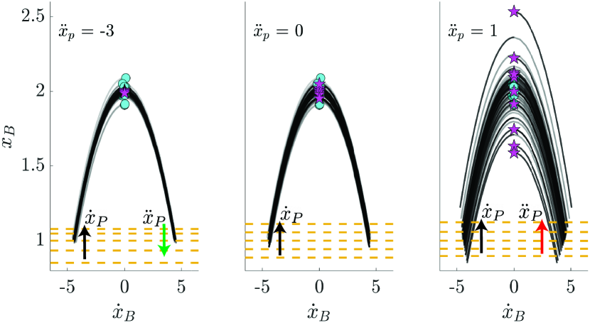
Figure 1: The paddle juggler system [6] has no control authority while the ball is in the air. The paddle acceleration at impact determines the convergence/divergence of the system from initial points (cyan dots) to the final states (magenta stars) after 5 cycles. This example underscores how hybrid event shaping can stabilize a periodic hybrid system.

II Preliminaries

II-A Hybrid systems

Hybrid systems are a class of dynamical systems which exhibit both continuous and discrete dynamics [10, 11]. Following the adaptation of [12] in [2], we define a $C^{r}$ hybrid dynamical system for continuity class $r\in\mathbb{N}_{>0}\cup\{\infty,\omega\}$ as a tuple $\mathcal{H}:=(\mathcal{J},\mathnormal{\Gamma},\mathcal{D},\mathcal{F},\mathcal{G},\mathcal{R})$ where:

1. $\mathcal{J}:=\{I,J,\ldots,K\}\subset\mathbb{N}$ is the set of discrete modes.

2. $\mathnormal{\Gamma}\subset\mathcal{J}\times\mathcal{J}$ is the set of discrete transitions forming a directed graph structure over $\mathcal{J}$.

3. $\mathcal{D}:=\amalg_{I\in\mathcal{J}}D_{I}$ is the collection of domains where $D_{I}$ is a $C^{r}$ manifold with corners [13].

4. $\mathcal{F}:=\amalg_{I\in\mathcal{J}}F_{I}$ is a collection of time-varying vector fields with control inputs $F_{I}:\mathbb{R}\times D_{I}\times U_{I}\rightarrow TD_{I}$ where $U_{I}$ is the space of allowable control inputs.

5. $\mathcal{G}:=\amalg_{(I,J)\in\mathnormal{\Gamma}}G_{(I,J)}(t)$ is a collection of guards where $G_{(I,J)}(t)\subset D_{I}\times U_{I}$ for each $(I,J)\in\mathnormal{\Gamma}$ is defined as a sublevel set of a $C^{r}$ function, i.e. $G_{(I,J)}(t)=\{(x,u)\in D_{I}\times U_{I}|g_{(I,J)}(t,x,u)\leq 0\}$.

6. $\mathcal{R}:\mathbb{R}\times\mathcal{G}\rightarrow\mathcal{D}$ is a $C^{r}$ map called the reset map that restricts as $R_{(I,J)}:=\mathcal{R}|_{G_{(I,J)}(t)}:G_{(I,J)}(t)\rightarrow D_{J}$ for each $(I,J)\in\mathnormal{\Gamma}$.

An execution of a hybrid system [12] begins at an initial state $x_{0}\in D_{I}$. With a particular input $u_{I}(t,x)$, the system follows the dynamics $F_{I}$ on $D_{I}$. If the system reaches the guard surface $G_{(I,J)}$, the reset map $R_{(I,J)}$ is applied and the system continues in domain $D_{J}$ with the corresponding dynamics defined by $F_{J}$. An execution of a hybrid system is defined over a hybrid time domain which is a disjoint union of intervals $\amalg_{j\in\mathcal{N}}[\underline{t}_{j},\bar{t}_{j}]$. The flow $\phi(t,t_{0},x_{0})$ describes how the system evolves from some initial time $t_{0}$ and state $x_{0}$ for some length of execution time $t$.

Hybrid systems may exhibit complex behaviors including sliding [14], branching [15], and Zeno phenomena where infinite transitions occur in finite time [16]. Following prior literature [17, 18, 19], we assume these behaviors do not occur, such that guard surfaces are isolated and intersected transversely [11, 12] and no Zeno executions occur. These assumptions are not generally detrimental to the validity of this theory to applications like legged locomotion.

II-B Saltation matrix

Hybrid systems can be divided into continuous domains and discrete hybrid events. For each of these components, the linearized variational equations [20] describe how perturbations of state at the beginning of the phase evolve to the end of the phase. In continuous domains, variational equations can be derived and discretized into a mapping $A_{I}(\bar{t}_{j}-\underline{t}_{j},\underline{t}_{j},x(\underline{t}_{j}))$ equivalent to the linearized discrete dynamics matrix in $x_{k+1}\approx A_{I}x_{k}+B_{I}u$ [20]. The variational equations of hybrid events are characterized by the saltation matrix $\Xi_{(I,J)}(\bar{t}_{i},x(\bar{t}_{i}),u(\bar{t}_{i}))$, which describes the transition between modes $I$ and $J$ that occurs at time $\bar{t}_{i}$ with $x(\bar{t}_{i})\in G_{(I,J)}$ and some input $u(\bar{t}_{i})$. The saltation matrix approximates the first-order change in perturbations in state before the hybrid event at $\delta x(\bar{t}_{i})$ to perturbations afterward $\delta x(\underline{t}_{i+1})$ [18] such that:

$$\delta x(\underline{t}_{i+1})=\Xi_{(I,J)}(\bar{t}_{i},x(\bar{t}_{i}),u(\bar{t}_{i}))\delta x(\bar{t}_{i})+\text{h.o.t.}$$ (1)

where h.o.t. represents higher order terms. Following the formulation from [18, 21], the saltation matrix is,

$$\Xi=D_{x}R+\frac{(F_{J}-D_{x}R\cdot F_{I}-D_{t}R)D_{x}g}{D_{t}g+D_{x}gF_{I}}$$ (2)

where

$$\Xi :=\Xi_{(I,J)}(\bar{t}_{i},x(\bar{t}_{i}),u(\bar{t}_{i})),\;R:=R_{(I,J)}(\bar{t}_{i},x(\bar{t}_{i}),u(\bar{t}_{i})),$$

$$g :=g_{(I,J)}(\bar{t}_{i},x(\bar{t}_{i}),u(\bar{t}_{i})),\;F_{I}:=F_{I}(\bar{t}_{i},x(\bar{t}_{i}),u(\bar{t}_{i})),$$

$$F_{J} :=F_{J}(\underline{t}_{i+1},R_{(I,J)}(\bar{t}_{i},x(\bar{t}_{i}),u(\bar{t}_{i}))$$

II-C Periodic Stability Analysis

A dynamical system has a periodic trajectory (orbit) with period $T$ if for some initial condition $x_{0}$, there exists a solution $\phi(t,t_{0},x_{0})$ where $\phi(t,t_{0},x_{0})=\phi(t+kT,t_{0},x_{0})$ for all $t$ and $k$ [19]. Perturbations $\delta x_{0}$ around $x_{0}$ can be mapped to perturbations $\delta x_{T}$ after period $T$ by a linearized mapping known as the monodromy matrix, $\Phi$ [22]:

$$\Phi=\frac{\partial\phi(T+t_{0},t_{0},x_{0})}{\partial x_{0}}$$ (3)

such that to the first order, $\delta x_{T}\approx\Phi\delta x_{0}$.

Following a formulation similar to [23], the monodromy matrix can be computed by sequentially composing the linearized variational equations in each continuous domain ($A$) and the saltation matrices ($\Xi$) at each hybrid event. For a hybrid periodic orbit with $N$ domains, the monodromy matrix can be formulated as:

$$\Phi=\Xi_{(N,1)}A_{N}\dots\Xi_{(2,3)}A_{2}\Xi_{(1,2)}A_{1}$$ (4)

The monodromy matrix determines local asymptotic orbital stability (which we refer to simply as stability). For nonautonomous systems, stability is determined by the maximum magnitude of the eigenvalues, $\max(|\lambda|)$ [19]. We refer to this as the stability measure, $\psi$, where a trajectory is stable when $\psi<1$. Autonomous systems always have an eigenvalue that is equal to 1 since for non-time varying dynamics, perturbations along the flow of the orbit will by definition map back to themselves after period $T$ [19]. Assuming non-convergence in this direction is allowable, $\psi$ for autonomous systems is based on the remaining eigenvalues.

III Methods

III-A Hybrid event shaping

Hybrid events can greatly affect the stability of an orbit due to the unbounded discontinuous changes that are made to perturbations. The saltation matrix allows for an explicit understanding of how to perform “hybrid event shaping” (HES), i.e. choosing hybrid event parameters (such as timing, state, input, and higher order “shape parameters”) to improve the stability of a periodic trajectory. The key insight is that hybrid event shaping introduces a generalizable method to stabilize hybrid systems that is independent of continuous-domain control, but that can work in concert with it.

In general, the open-loop continuous variational equations of a hybrid system are functions of initial and final time, initial state, and system dynamics. However, it is challenging to alter any of these parameters because changes will propagate through the rest of the trajectory and periodicity may be violated, though we present a trajectory optimization method below to handle this. The saltation matrix is a function of nominal event time, state and dynamics, but additionally may be a function of higher order shape parameters $h$ that do not influence the dynamics of the system. These parameters arise from the derivatives of the guards ($D_{x}g$ and $D_{t}g$) and reset maps ($D_{x}R$ and $D_{t}R$) but are not present in the guard, reset map, or vector field definitions themselves. Therefore, shape parameters have absolutely no effect on the nominal trajectory and can be chosen completely freely.

One example of a shape parameter is the angular velocity of a massless leg of a spring-loaded inverted pendulum. Since a massless leg does not induce any torque in the air or forces at touchdown, only the position of the leg at touchdown affects the trajectory of the body. However, leg velocity appears in the saltation matrix and has a significant effect on orbital stability [7].

For more complex models of robots, there may not be any physical shape parameters that can be tuned. For example, legged robots with non-massless legs can not vary leg velocity at impact without also changing its trajectory. These cases can be handled by running a trajectory optimization at the same time as applying HES, as we show in Sec. III-E, or by adding additional virtual hybrid events.

III-B Virtual hybrid events

Certain control systems naturally have discontinuities in control inputs, such as bang-bang control, sliding mode control, or systems with actuators that have discretized (i.e. on-off) inputs. These discontinuities in control can cause an instantaneous change in the dynamics of the system, resulting in a virtual (as opposed to physical) hybrid event. Virtual hybrid events act no differently than physical hybrid events and induce saltation matrices with shape parameters to be tuned for stability. Even for systems where discontinuous control inputs are not necessary, the addition of virtual saltation matrices and shape parameters allows for a greater authority to improve stability.

III-C Stability measure derivative

Our goal is to determine the optimal choice of hybrid event parameters that minimizes the stability measure of a trajectory. Since directly computing eigenvalues in closed-form is not generally feasible, one solution is to use numerical methods to perform optimization [24]. However, this strategy becomes untenable for high dimensional problems. Instead, by using the saltation matrix formulation (2), derivatives of the stability measure can be directly computed, allowing for the use of more efficient optimization methods and making the problem much more tractable.

Assuming that the monodromy matrix $\Phi$ depends continuously on each shape parameter $h_{n}$, the eigenvalues of $\Phi$ are always continuous with respect to $h_{n}$ [25]. For a diagonalizable $\Phi$, the derivative of the eigenvalues with respect to $h_{n}$ can be computed in closed form [26]. Assume that matrix $\Phi(h_{n})$ has simple (non-repeating) eigenvalues, $\lambda_{1},\ldots,\lambda_{N}$, and let $\boldsymbol{j}_{i}$ and $\boldsymbol{k}_{i}$ denote the left and right eigenvectors associated with $\lambda_{i}$. Then the derivative $\frac{d\lambda_{i}}{dh_{n}}$ is:

$$\frac{d\lambda_{i}}{dh_{n}}=\boldsymbol{k}_{i}^{\prime}\frac{d\Phi}{dh_{n}}\boldsymbol{j}_{i}$$ (5)

For matrices with eigenvalues that repeat, the derivatives of the repeated eigenvalues can be calculated similarly with a matrix of associated eigenvectors [26].

$\frac{d\Phi}{dh_{n}}$ can be found using the derivative product rule, which simplifies if each shape parameter only appears in one saltation matrix. We make this assumption here to improve computational efficiency, but it is not required generically. Without loss of generality, take $\frac{d\Xi_{(1,2)}}{dh_{n}}\neq 0$, so that:

$$\frac{d\Phi}{dh_{n}}=\Xi_{(N,1)}A_{N}\dots A_{2}\frac{d\Xi_{(1,2)}}{dh_{n}}A_{1}$$ (6)

Substituting (6) into (5) allows us to compute the derivative of the stability measure with respect to each of the shape parameters. Eq. (5) is not valid for non-diagonalizable monodromy matrices. However, the guaranteed continuity of the stability measure allows for finite-difference methods to be used in any non-diagonalizable cases.

The derivative computation from (6) can be adapted for changes in $x$ and $t$ as well. Without loss of generality, consider again $\Xi_{(1,2)}$. For hybrid event time $t_{(1,2)}$, the derivative $\frac{d\Xi_{(1,2)}}{dt_{(1,2)}}$ can be computed in closed-form. Additionally, the derivatives $\frac{dA_{1}}{dt_{(1,2)}}$ and $\frac{dA_{2}}{dt_{(1,2)}}$ are non-zero and can be computed through standard methods [27]. The product rule expansion of $\frac{d\Phi}{dt_{(1,2)}}$ consists of additional terms compared to (6) but otherwise can be computed similarly. $\frac{d\Phi}{dx_{(1,2)}}$ for hybrid event state $x_{(1,2)}$ can be computed this same way.

III-D Shape parameter stability optimization

Optimization techniques [28] are able to select optimal hybrid event parameters that minimize the stability measure. Two optimization methods are presented here: the first optimizing the shape parameters without affecting the dynamics of the nominal orbit, and the second optimizing both the hybrid events and periodic orbit simultaneously.

Shape parameters are powerful because they do not appear in the dynamics of the system and have no effect on the nominal trajectory. This means that for a given periodic trajectory, the shape parameters can be chosen freely. We use an optimization framework to choose these shape parameters with the goal of optimizing the stability measure $\psi(\Phi(h))$ of a trajectory,

$$\begin{array}[]{cl}\underset{h_{1:M}}{\operatorname{minimize}}&\psi(\Phi(h))\end{array}$$ (7)

The ability to compute derivatives of the stability measure allows for this optimization to be more computationally efficient. The examples below show how this optimization method is able to reproduce swing leg retraction in a one-legged hopper system by determining optimal inputs of shape parameters to minimize the stability measure.

III-E Trajectory optimization with hybrid event shaping

Some systems do not have shape parameter terms in their saltation matrices or do not have enough to sufficiently improve stability. In these cases, we can change the trajectory of the system itself so that the timing, state, and input parameters of the continuous variational matrices and saltation matrices improve stability properties. However, it must be ensured that the dynamics, periodicity, and other constraints of the system are obeyed.

Trajectory optimization methods are a class of algorithms that aim to minimize a cost function while satisfying a set of constraints [29]. For dynamical systems, these costs are generally functions of state and inputs, with constraints imposed on system dynamics and any other physical limits [30]. For specific problems, other aspects of the system may be added into the cost or constraint functions such as design parameters or minimizing time [31, 32]. Here we propose including the stability measure in the cost function to search for optimally stable trajectories. Eq. (8) gives the simplest form of this trajectory optimization problem, with periodicity and dynamics constraints being enforced, where dynamics constraints obey continuous dynamics in each domain and reset mappings at each hybrid event [33]. Additional costs and constraints may be included such as reference tracking costs, input costs, and any physical constraints. We solve this problem using a direct collocation optimization with a multi-phase method to handle hybrid events [29, 30, 34].

$$\begin{array}[]{cl}\underset{x_{1:N},u_{1:N-1},t_{1:N-1},h_{1:M}}{\operatorname{minimize}}&\psi(\Phi(x,t,h))\\ \text{ subject to }&x_{N}=x_{1}\\ &x_{i+1}=\phi(t_{i+1}-t_{i},t_{i},x_{i})\end{array}$$ (8)

IV Examples and Results

Here we demonstrate how HES can improve the stability of periodic trajectories for a variety of hybrid systems without any use of continuous-domain feedback control. While continuous-domain feedback could be implemented into any of these systems and should be in practice, these examples emphasize the stabilization capabilities of HES alone.

The first two examples describe how previously discovered results, paddle juggling [6] and swing leg retraction [7], fit into an HES framework. The final example demonstrates how HES can be used even without any shape parameters and how virtual hybrid events can help stabilize a complicated biped walking system.

IV-A Paddle juggler

The paddle juggler system [6], bouncing a ball with a paddle, is known to be stabilized by impacting the ball with a paddle acceleration in a range of negative values, (10), Fig. 1. The system state consists of the ball’s vertical position and velocity such that $x=[x_{B},\dot{x}_{B}]^{T}$. This periodic hybrid system can be defined with two hybrid domains (descent and ascent) connected by two guards (impact and apex). The domain $D_{1}$ represents the ball’s aerial descent phase where $\dot{x}_{B}<0$ and $D_{2}$ represents the ball’s aerial ascent phase where $\dot{x}_{B}>0$. The guard set $g_{(1,2)}:=x_{B}-x_{P}\leq 0$ is defined when the ball impacts the paddle, where the paddle follows a twice differentiable trajectory $x_{P}(t)$. The reset map $R_{(1,2)}$ is defined by a partially elastic impact law, $R_{(1,2)}([x_{B},\dot{x}_{B}]^{T})=[x_{B},(1+\alpha)\dot{x}_{P}-\alpha\dot{x}_{B}]^{T}$, with a coefficient of restitution $\alpha$. The continuous dynamics in both domains follow unactuated ballistic motion: $\mathcal{F}_{1}=\mathcal{F}_{2}=[\dot{x}_{B},-g]^{T}$, where $g$ is the acceleration due to gravity.

Using these definitions, the saltation matrix (2) between domains $1$ and $2$ is constructed:

$$\Xi_{(1,2)}=\begin{bmatrix}-\alpha&0\\ \frac{(1+\alpha)\cdot(\ddot{x}_{P}+g)}{\dot{x}_{P}-\dot{x}_{B}}&-\alpha\end{bmatrix}$$ (9)

Observe that $\ddot{x}_{P}$ appears in the saltation matrix even though it does not appear anywhere in the definition of the guards, reset maps, or vector fields of the system, making it a shape parameter that can be chosen independently of the periodic orbit.

The guard set $g_{(2,1)}:=\dot{x}_{B}\leq 0$ is defined when the ball reaches the apex of its ballistic motion. Its reset map $R_{(2,1)}$ is identity and there is no change in dynamics. Thus, $\Xi_{(2,1)}$ is identity and has no effect on the variations of the system.

The continuous variational matrices of the system can be written exactly in closed form: $A_{1}(T)=A_{2}(T)=\bigl{[}\begin{smallmatrix}1&T/2\\ 0&1\end{smallmatrix}\bigr{]}$ where $T$ is the total time spent in the air and also the period of the system. The periodicity of the system means the ball spends an equal time, $T/2$, ascending as descending.

The monodromy matrix, $\Phi$ is constructed by composing together the continuous variational matrices and saltation matrices such that $\Phi=\Xi_{(2,1)}A_{2}\Xi_{(1,2)}A_{1}$.

For a given periodic bouncing trajectory, the monodromy matrix $\Phi$ is almost fully defined except for the shape parameter, $\ddot{x}_{P}$ in $\Xi_{(1,2)}$. Given the 2-dimensional state space of this problem, the eigenvalues for any given $\ddot{x}_{P}$ value can be solved for explicitly. We can then solve exactly for where $\psi(\ddot{x}_{P})<1$, giving a stable region of:

$$-2g\frac{1+\alpha^{2}}{(1+\alpha)^{2}}<\ddot{x}_{P}<0$$ (10)

This is confirmed in [6], where the simple dynamics of the system allowed the return map to be computed explicitly without the saltation matrix. However, that computation is generally not possible for more complex dynamics.

IV-B 2D hopper

The spring-loaded inverted pendulum (SLIP) is a popular model for dynamic legged locomotion [35, 36, 37]. This simple hopper model is effective at capturing dynamic properties of animal and robot locomotion [38] and has been used as a test bed for hybrid controllers [39].

IV-B1 2D hopper hybrid model

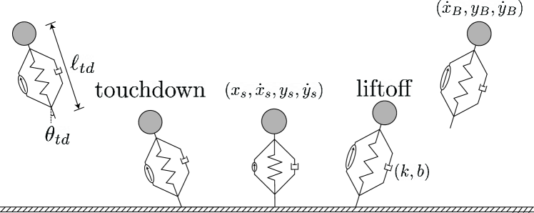
Figure 2: SLIP-like system with actuator and damper in parallel.

Consider a point mass body with a massless leg consisting of a spring, damper, and linear actuator all in parallel, Fig. 2. This system has two domains (flight and stance) connected by two guards (touchdown and liftoff). The actuator is activated while in the air to preload the spring, but immediately releases at touchdown and provides no forces during stance. For a periodic trajectory to occur, the actuator must preload the same amount of energy that is dissipated by the damper during stance. The only control authority that exists is of the leg angle in the air, which only affects the dynamics of the body at touchdown.

During flight ($D_{1}$), the state of the hopper is represented by the horizontal velocity, vertical position, and vertical velocity of the body: $x=[\dot{x}_{B},y_{B},\dot{y}_{B}]^{T}$. Horizontal position is not included because it is not periodic. During stance, the body position $x_{s}$ and $y_{s}$ is defined with the toe at the origin. Horizontal position is added back into the state of the hopper such that $x=[x_{s},\dot{x}_{s},y_{s},\dot{y}_{s}]^{T}$. In flight, the dynamics of the body follow ballistic motion, while in stance there are also forces applied by the spring and damper.

The touchdown guard is defined by the preload length of the leg $\ell_{td}$ and angle of the leg $\theta_{td}$ such that $g_{(1,2)}:=y_{B}-\ell_{td}\cos(\theta_{td})$. The liftoff guard is crossed when the force exerted by the spring-damper, $F_{sd}$, becomes zero: $g_{(2,1)}:=F_{sd}$. There is no change in physical state of the system at the hybrid events and the reset maps only characterize the change in coordinates between domains.

Given a set of model parameters, a trajectory from an initial condition depends only on $\ell_{td}$ and $\theta_{td}$. $\ell_{td}$ is held fixed, but $\theta_{td}$ is modulated from its nominal position $\overline{\theta}_{td}$ at time $\bar{t}_{td}$ in two ways. A proportional feedback term with gain K is added to stabilize the forward velocity of the system around a nominal $\overline{\dot{x}}$ and angular velocity $\dot{\theta}$ of the massless leg is also free to be chosen. $K$ and $\dot{\theta}$ are shape parameters that can be used to stabilize this system.

$$\theta_{td}=\overline{\theta}_{td}+K(\dot{x}-\overline{\dot{x}})+\dot{\theta}(t-\bar{t}_{td})$$ (11)

IV-B2 2D hopper HES results

For a chosen initial apex height of $2.5$ with a forward velocity of $2$, $\ell_{td}$ and $\overline{\theta}_{td}$ were solved for to produce a nominal orbit, though the following results generalize for any choice of feasible values.

With fixed shape parameters $[K,\dot{\theta}]=[0,0]$, the system is highly unstable. $K$ and $\dot{\theta}$ can be optimized following (7) to improve the stability of this orbit. Doing so results in optimal shape parameters $[K,\dot{\theta}]=[0.129,-0.015]$ that stabilize the trajectory, Table I. Setting $\dot{\theta}=-0.015\text{ rad/s}$ is a slow retraction rate, but there exists an interval of values $\dot{\theta}\in(-0.5892,-0.015)$ that give equivalently minimal stability measures for a fixed $K$ value.

TABLE I: Stability measures of 2D hopper trajectories without and with optimized shape parameters.

Shape parameters	K	$\dot{\theta}$	Stability Measure
Zero	0	0	13.756
Optimal (zero seed)	0.129	-0.015	0.948
Optimal (alternate seed)	0.129	-0.589	0.948

The results were confirmed in simulation by initializing 20 perturbed points in a $0.1$ radius ball around the nominal initial condition. Each of these trials was simulated for $100$ steps and the error (2-norm of the difference in perturbed state $x$ and nominal state $\bar{x}$) at apex was recorded at each step, Fig. 3. The zero shape parameter trajectories are not shown in the figure as every trial diverged within just 5 steps.

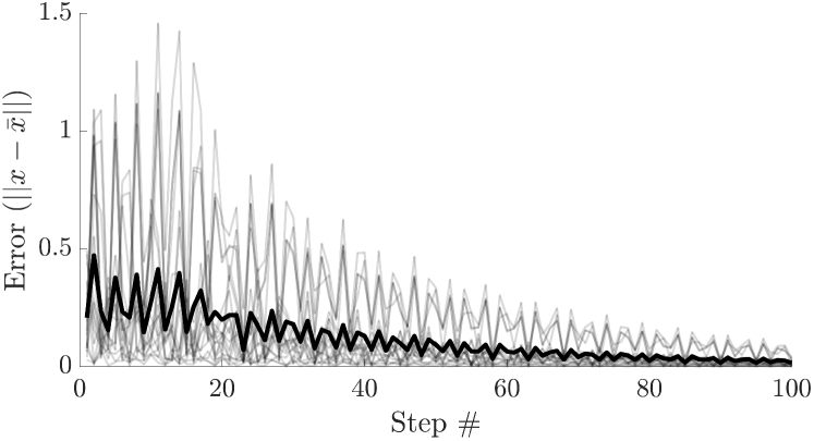
Figure 3: Error of perturbed initial states for the 2D hopper asymptotically decrease to zero. Transparent lines represent each of the 20 trials, while the bold line represents average error at each step. Convergence is neither monotonic nor very fast, but this is expected with asymptotic stability.

IV-B3 2D Hopper Discussion

The feedback term of (11) is based on the Raibert stepping controller [40], which was utilized to great success for stabilizing early running robots. Other works have found that this simple controller is effective on more complex models [41].

Another stabilizing property of legged locomotion that has been studied is swing-leg retraction [7, 24, 42]. It was noted in [7] that a 2D SLIP was able to run stably if it impacted the ground within a range negative angular leg velocities $\dot{\theta}$.

The results of a negative $\dot{\theta}$ and positive $K$ agree with qualitative expectations from [7] and [40]. While a formal equivalency is yet to be proven, this is significant because the HES shape parameter optimization has no a priori knowledge that would bias its results to match these works. HES synthesizes two independently generated controllers and produces shape parameter values that stabilize an orbit. This evidence supports the potential for HES to explore other stabilizing shape parameters that are not as well studied.

IV-C Walking biped trajectory optimization

For a legged system with non-massless legs, the leg velocity shape parameter disappears as it is no longer independent of the trajectory. Without shape parameters, an HES trajectory optimization can choose timing, state, and input parameters along with injecting virtual hybrid events to discover stable orbits.

IV-C1 Walking biped hybrid model

In this example, we consider a fully-actuated compass walker [43] with knees, Fig. 4. This biped model consists of two legs connected by an actuated hip joint. Each leg is separated into two sections, the upper leg (thigh) and lower leg (shank), which are connected by an actuated knee joint that has a hard stop when the thigh and shank are aligned. The ankles are also actuated.

We restrict the gaits to be left-right symmetric and exclusively consist of single stance phases. The stance leg is locked such that its shank and thigh are aligned with each other until liftoff. There are 3 points of actuation at the hip, swing knee, and stance ankle. The state space is defined by three angles relative to vertical: stance leg, swing thigh, and swing shank, denoted $(\theta_{1},\theta_{2},\theta_{3})$.

This system has two domains. $D_{1}$ is the unlocked knee domain where the swing leg thigh and shank can swing freely while we enforce that $\theta_{3}<\theta_{2}$. $D_{2}$ is the locked knee domain where the thigh and shank are constrained to be aligned with each other ($\theta_{2}=\theta_{3}$). In this domain, there are only two actuators because the swing knee can no longer exert torque. The dynamics of this model are described in [43].

The kneestrike guard set, between the unlocked and locked knee domains, is $g_{(1,2)}:=\theta_{2}-\theta_{3}$ and the touchdown or toestrike guard set is $g_{(2,1)}:=\theta_{1}+\theta_{2}$. The reset maps at kneestrike and toestrike are also computed in [43].

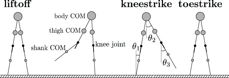
Figure 4: Biped walker system with kneestrike and toestrike hybrid events.

We add discrete changes in the inputs that induce virtual hybrid events to analyze their utility in stabilizing walking trajectories. Specifically, we choose to include 5 virtual hybrid events in $D_{1}$ and 2 more virtual hybrid events in $D_{2}$, where the values of inputs between virtual hybrid events are decision variables for the optimization. The virtual guard functions are chosen such that $g_{v_{i}}:=\theta_{2}-\theta_{3}+p_{i}$ for the first 5 virtual hybrid events and $g_{v_{i}}:=\theta_{1}+\theta_{2}+p_{i}$ for the last 2 virtual hybrid events for some offset $p_{i}$ that is also chosen by the optimization.

A direct collocation method was used with the cost consisting of the stability measure and a regularization on the input. Dynamics and periodicity constraints were included along with a ground penetration constraint. The initial conditions of the system, given as the state after touchdown, were allowed to vary within a bounded range.

IV-C2 Walking biped HES results

In this experiment, three trajectories were compared to examine how HES can generate stable trajectories and the effect that virtual hybrid events have in further improving stability. A trajectory without HES was produced as a control, with its objective to minimize energy expended by using just an input regularization term in the cost. This minimum energy (ME) trajectory is comparable to how conventional robot locomotion trajectories are generated. Two HES trajectories were generated, one with virtual hybrid events (HES w/ VHE) and one without (HES w/o VHE).

The ME trajectory is highly unstable, while the both HES trajectories are stable with the trade off of a higher input cost. Specifically, HES w/ VHE has the lowest stability measure and highest energy cost, whereas HES w/o VHE was in between for both stability and cost, Table II.

TABLE II: Stability results for the walking biped optimization.

Trajectory	Stability Measure	Energy Cost
ME	7.8123	0.985
HES w/o VHE	0.4715	1.337
HES w/ VHE	0.3266	3.450

The stability properties of the generated trajectories were confirmed through simulation. 50 trials of each trajectory were initialized with perturbations in position and velocity between $(-0.01,0.01)$. Over a sequence of 10 steps, the state error at each step was tracked for each trial. Fig. 5 shows that after 10 steps, the HES trajectories have nearly converged back to the nominal trajectory whereas the ME trajectories diverge quickly. The HES w/ VHE trajectory converges to a smaller error after 10 steps compared to the HES w/o VHE trajectory, which supports the findings of the stability measure.

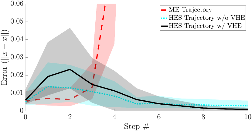
Figure 5: Error of perturbed Minimum Energy (ME), Hybrid Event Shaping without virtual hybrid events (HES w/o VHE) and HES w/ VHE trajectories over several steps. Bold lines show average error at each step and shaded regions indicate $\pm 1$ standard deviation. ME trajectories becomes highly divergent within 4 steps, while both HES trajectories appear convergent after 10 steps. The initial increase in error of the HES trajectories is allowable and is not considered by the stability measure.

V Conclusion

While the idea of hybrid event control is not novel, hybrid event shaping provides a generalized method to analyze the stability of hybrid orbits and select hybrid event parameters to optimize stability. HES unifies results of previous simple hybrid event controllers while also being compatible with trajectory optimization techniques to produce stable trajectories for complex systems. HES computes the derivative of the stability measure, improving computational efficiency compared to previous stability optimization methods. Compared to previous work, HES does not rely on human observation and tuning to design stabilizing hybrid event parameters.

In this work, there was no use of continuous-domain feedback that is commonly utilized in hybrid systems control. We believe that hybrid event shaping is one aspect that can be used in conjunction with continuous-domain feedback to improve the success rate of robots performing dynamic behaviors in real-world settings. This is not be prohibitively complex because saltation matrices are not affected by feedback control laws in the continuous domains. In the future, we aim to synthesize HES methods with continuous-domain feedback control to produce even more stable closed-loop trajectories. We also found that virtual hybrid events may have utility in stabilizing hybrid orbits, but design factors such as how many virtual hybrid events to insert and when to insert them merit further investigation.

References

- [1] B. Altın, P. Ojaghi, and R. G. Sanfelice, “A model predictive control framework for hybrid dynamical systems,” IFAC-PapersOnLine, vol. 51, no. 20, pp. 128–133, 2018.
- [2] N. J. Kong, G. Council, and A. M. Johnson, “iLQR for piecewise-smooth hybrid dynamical systems,” in IEEE Conference on Decision and Control, December 2021, to appear.
- [3] W. Yang and M. Posa, “Impact invariant control with applications to bipedal locomotion,” arXiv preprint arXiv:2103.06907, 2021.
- [4] S. Burden, S. Revzen, and S. Sastry, “Dimension reduction near periodic orbits of hybrid systems,” in IEEE Conference on Decision and Control, September 2011.
- [5] G. Council, S. Yang, and S. Revzen, “Deadbeat control with (almost) no sensing in a hybrid model of legged locomotion,” in International Conference on Advanced Mechatronic Systems, 2014, pp. 475–480.
- [6] D. Sternad, M. Duarte, H. Katsumata, and S. Schaal, “Bouncing a ball: Tuning into dynamic stability,” Journal of Experimental Psychology: Human Perception and Performance, vol. 27, pp. 1163–84, 11 2001.
- [7] A. Seyfarth, H. Geyer, and H. Herr, “Swing-leg retraction: a simple control model for stable running,” Journal of Experimental Biology, vol. 206, no. 15, pp. 2547–2555, 2003.
- [8] M. M. Ankaralı, U. Saranlı, and A. Saranlı, “Control of underactuated planar hexapedal pronking through a dynamically embedded slip monopod,” in IEEE International Conference on Robotics and Automation, 2010, pp. 4721–4727.
- [9] K. Green, R. Hatton, and J. Hurst, “Planning for the unexpected: Explicitly optimizing motions for ground uncertainty in running,” in IEEE International Conference on Robotics and Automation, May 2020.
- [10] A. van der Schaft and J. Schumacher, “Complementarity modeling of hybrid systems,” IEEE Transactions on Automatic Control, vol. 43, no. 4, 1998.
- [11] J. Lygeros, K. H. Johansson, S. Simic et al., “Dynamical properties of hybrid automata,” IEEE Transactions on Automatic Control, 2003.
- [12] A. M. Johnson, S. A. Burden, and D. E. Koditschek, “A hybrid systems model for simple manipulation and self-manipulation systems,” The International Journal of Robotics Research, vol. 35, no. 11, pp. 1354–1392, 2016.
- [13] D. Joyce, “On manifolds with corners,” in Advances in Geometric Analysis, ser. Advanced Lectures in Mathematics. International Press of Boston, Inc., 2012, vol. 21, pp. 225–258.
- [14] M. Jeffrey, “Dynamics at a switching intersection: Hierarchy, isonomy, and multiple sliding,” SIAM Journal on Applied Dynamical Systems, vol. 13, pp. 1082–1105, 07 2014.
- [15] S. N. Simić, K. H. Johansson, S. Sastry, and J. Lygeros, “Towards a Geometric Theory of Hybrid Systems,” in Hybrid Systems: Computation and Control, ser. Lecture Notes in Computer Science, N. Lynch and B. H. Krogh, Eds. Berlin, Heidelberg: Springer, 2000, pp. 421–436.
- [16] J. Zhang, K. H. Johansson, J. Lygeros, and S. Sastry, “Dynamical systems revisited: Hybrid systems with zeno executions,” in Hybrid Systems: Computation and Control. Springer Berlin Heidelberg, 2000.
- [17] M. Aizerman. and F. Gantmacher, “Determination of Stability by Linear Approximation of a Periodic Solution of a System of Differential Equations With Discontinuous Right-hand Sides,” The Quarterly Journal of Mechanics and Applied Mathematics, vol. 11, no. 4, pp. 385–398, 01 1958. [Online]. Available: https://doi.org/10.1093/qjmam/11.4.385
- [18] S. A. Burden, T. Libby, and S. D. Coogan, “On contraction analysis for hybrid systems,” arXiv preprint arXiv:1811.03956, 2018.
- [19] R. Leine and H. Nijmeijer, Dynamics and Bifurcations of Non-Smooth Mechanical Systems. Springer-Verlag Berlin Heidelberg, 2004.
- [20] M. Hirsch, S. Smale, and R. Devaney, Differential Equations, Dynamical Systems, and an Introduction to Chaos. Academic Press, 2012.
- [21] P. Müller, “Calculation of lyapunov exponents for dynamic systems with discontinuities,” Chaos, Solitons & Fractals, vol. 5, no. 9, pp. 1671–1681, 1995.
- [22] X. Wang and J. K. Hale, “On monodromy matrix computation,” Computer Methods in Applied Mechanics and Engineering, vol. 190, no. 18, 2001.
- [23] H. Asahara and T. Kousaka, “Stability analysis using monodromy matrix for impacting systems,” IEICE Transactions of Fundamentals of Electronics, Communications, and Computer Science, vol. E101-A, no. 6, 2018.
- [24] J. G. D. Karssen, M. Haberland, M. Wisse, and S. Kim, “The optimal swing-leg retraction rate for running,” in IEEE International Conference on Robotics and Automation, 2011, pp. 4000–4006.
- [25] E. Tyrtyshnikov, A Brief Introduction to Numerical Analysis. Birkhäuser Basel, 1997.
- [26] P. Lancaster, “On eigenvalues of matrices dependent on a parameter,” Numerische Mathematik, 1964.
- [27] H. Khalil, Nonlinear Systems. Pearson, 2002.
- [28] J. Nocedal and S. Wright, Numerical Optimization. Springer, 2006.
- [29] M. Kelly, “An introduction to trajectory optimization: How to do your own direct collocation,” SIAM Review, vol. 59, no. 4, pp. 849–904, 2017.
- [30] O. Von Stryk and R. Bulirsch, “Direct and indirect methods for trajectory optimization,” Annals of Operations Research, vol. 37, pp. 357–373, 12 1992.
- [31] C. R. Hargraves and S. W. Paris, “Direct trajectory optimization using nonlinear programming and collocation,” Journal of Guidance, Control, and Dynamics, vol. 10, no. 4, pp. 338–342, 1987.
- [32] K. Mombaur, R. Longman, H. Bock, and J. Schlöder, “Open-loop stable running,” Robotica, vol. 23, pp. 21–33, 01 2005.
- [33] O. V. Stryk, “User’s guide for DIRCOL (version 2.1): a direct collacation method for the numerical solution of optimal control problems,” in Technische Universitat Darmstadt, November 1999.
- [34] J. T. Betts, Practical Methods for Optimal Control and Estimation Using Nonlinear Programming, Second Edition, 2nd ed. SIAM, 2010.
- [35] T. A. McMahon and G. C. Cheng, “The mechanics of running: How does stiffness couple with speed?” Journal of Biomechanics, vol. 23, pp. 65–78, 1990.
- [36] P. Holmes, R. J. Full, D. E. Koditschek, and J. Guckenheimer, “The dynamics of legged locomotion: Models, analyses, and challenges,” SIAM Review, vol. 48, no. 2, pp. 207–304, 2006.
- [37] A. Seyfarth, H. Geyer, M. Günther, and R. Blickhan, “A movement criterion for running,” Journal of Biomechanics, vol. 35, no. 5, pp. 649–655, 2002.
- [38] R. J. Full and D. E. Koditschek, “Templates and anchors: neuromechanical hypotheses of legged locomotion on land,” Journal of Experimental Biology, vol. 202, no. 23, pp. 3325–3332, 12 1999.
- [39] J. Seipel and P. Holmes, “A simple model for clock-actuated legged locomotion,” Regular and Chaotic Dynamics, vol. 12, no. 5, Oct. 2007.
- [40] M. Raibert, H. Brown, and M. Chepponis, “Experiments in balance with a 3D one-legged hopping machine,” The International Journal of Robotics Research, vol. 3, no. 2, pp. 75–92, 1984.
- [41] I. Poulakakis and J. W. Grizzle, “The spring loaded inverted pendulum as the hybrid zero dynamics of an asymmetric hopper,” IEEE Transactions on Automatic Control, vol. 54, no. 8, pp. 1779–1793, 2009.
- [42] Y. Blum, S. Lipfert, J. Rummel, and A. Seyfarth, “Swing leg control in human running,” Bioinspiration & Biomimetics, vol. 5, June 2010.
- [43] V. Chen, “Passive dynamic walking with knees: A point foot model,” Master’s thesis, Massachusetts Institute of Technology, 2007.