A mixture model for determining SARS-Cov-2 variant composition in pooled samples

Abstract.

Despite of the fast development of highly effective vaccines to control the current COVID$-$19 pandemic, the unequal distribution and availability of these vaccines worldwide and the number of people infected in the world lead to the continuous emergence of SARS-CoV-2 (Severe Acute Respiratory Syndrome coronavirus 2) variants of concern. It is likely that real-time genomic surveillance will be continuously needed as an unceasing monitoring tool, necessary to follow the spillover of the disease spread and the evolution of the virus. In this context, new genomic variants of SARS-CoV-2 that may emerge as a response to selective pressure, including variants refractory to current vaccines, makes genomic surveillance programs tools of utmost importance. Here propose a statistical model for the estimation of the relative frequencies of SARS-CoV-2 variants in pooled samples. This model is built by considering a previously defined selection of genomic polymorphisms that characterize SARS-CoV-2 variants. The methods described here support both raw sequencing reads for polymorphisms-based markers calling and predefined markers in the VCF format. Results obtained by using simulated data show that our method is quite effective in recovering the correct variant proportions. Further, results obtained by considering longitudinal data from wastewater samples of two locations in Switzerland agree well with those describing the epidemiological evolution of COVID-19 variants in clinical samples of these locations. Our results show that the described method can be a valuable tool for tracking the proportions of SARS-CoV-2 variants.

1. Introduction

The astonishing speed seen for the global spread of COVID-19 has prompted a large global effort to control this outbreak. The first complete SARS-CoV-2 genome was published on January 05, 2020 by [WZY⁺20]. Thenceforth, SARS-CoV-2 sequences recovered from patients from most countries have been made available to the scientific community [MHG21], allowing a better understanding of the geographical and temporal spreading of SARS-CoV-2, including the indication of non-synonymous genomic variants that may explain the increased replication rate and immune escaping of some variants [ZSZ⁺21] Today, the Global Initiative on Sharing Avian Influenza Data (GISAID) database is arguably the primary archive for SARS-CoV-2 genome sequences [Max21].

Although vaccination is the most effective means of preventing COVID-19 illnesses and related deaths [CBH⁺21], additional efforts employing genomic surveillance have proven to be a useful tool for guiding upcoming measures to control virus transmission [RAS⁺21, GL18]. The sequencing of Viral RNA genomes directly recovered from wastewater has recently gained attention for providing an opportunity to assess circulating viral lineages [BOWI⁺21, SAB⁺21, FKH⁺21, PQBC⁺20, JDT⁺21]. These studies take advantage of shotgun-based sequencing protocols [ACA⁺17] followed by the most typical computational workflows to unveil the genomic diversity present in a given sample, consisting of (1) sequencing quality profiling; (2) removal of host/rRNA data; (3) assembly of reads; and (4) attribution of taxonomy [ACA⁺17, HLZ⁺21]. It is also be clear that this approach can be applied in other sources of urban metagenomic surveilance [D⁺21].

The main contribution of this article consists in the development of a statistical model to infer the relative proportions and frequencies of the genomic variants of SARS-CoV-2 present in varying amounts in a given sample. This task is far from trivial as the sequencing reads deriving from a sample consist of relatively short sequences ($\approx 100-200$ bases long) that can be mapped to multiple variants of the virus. The sequencing reads derived from a given locus of the viral genome may be different across the individuals of the same variant due to intra-clade variation. Also, the small proportion of sequenced reads likely to align to the SARS-CoV-2 in the midst of a complex mixture of other RNAs (human, viral, bacterial and others) may lead to reduced vertical coverage of the viral genome, therefore decreasing the likelihood of an effective variant monitoring.

Here, we propose a viral composition deconvolution approach based on the relative frequencies of genomic polymorphic markers found in SARS-CoV-2 variants. These markers, either Single Nucleotide Polymorphisms (SNPs) or INsertion or DELetion of bases (INDELs), are selected from public SARS-CoV-2 data [SM17, TTH⁺21] and their presence/absence in known SARS-CoV-2 variants is used to fit a mixture model to viruses, derived from different subjects, found in a complex mixture. Following this, our method calculates a maximum likelihood estimate of the relative contributions of SARS-CoV-2 variants to the pool. The performance of the test was evaluated in simulated and real data. Our analysis using 122 sequencing data-points from wastewater treatment plants collected in Switzerland, show close correlation with epidemiological trends of COVID-19 in that region, which demonstrates the utility of this approach to guide public policies

2. Variant composition model

Our model is built over a previously defined selection of genomic polymorphisms, which characterize SARS‑CoV‑2 variants, and a matrix $P$ of ‘variant signatures’. Formally, let $P=(P_{ij})$ be a $s\times v$ matrix such that $P_{ij}$ corresponds to the probability of finding an alternate sequence at polymorphism $i$ from variant $j$. Details about the selection of polymorphisms of interest and the construction of $P$ are provided in Section 3.1. Given the matrix $P$ and a data sample containing the counts of DNA fragment readings aligned to the respective polymorphic loci at SARS-CoV-2 genome, we aim at estimating the vector $w=(w_{1},w_{2},\ldots,w_{v})$ of the relative compositions of SARS-CoV-2 variants in the sample, such that

(1) $$0\leq w_{j}\leq 1,\qquad\sum_{j=1}^{v}w_{j}=1.$$

Let $\{\text{Poly}_{i}\}$, $i=1,2,\ldots,v$, be the set of polymorphisms of interest. The data provided by a sample consists of counts of reads supporting the reference sequence $c_{i}^{r}$ and those supporting an alternate sequence, $c_{i}^{a}$ at each $\text{Poly}_{i}$. Two crucial remarks about the data are that the coverage, that is $c_{i}^{a}+c_{i}^{r}$, may vary among polymorphisms, and that the data does not shows which variants account for the actual observed counts $c_{i}^{r}$ and $c_{i}^{a}$. The latter occurs because:

• the reads that constitute the sample are relatively small segments of the viral genomes,

• variants may share few $\text{Poly}_{i}$ events,

• there is random variability among the polymorphisms across the individuals of the same variant.

A relation between counts and variants is made by introducing the latent variables $Z_{ij}^{r}$ and $Z_{ij}^{a}$, representing respectively the counts of reads bearing the reference sequence for a $\text{Poly}_{i}$ event originating from variant $j$ and those bearing the reference base at the position $i$ from the variant $j$. In this case

(2) $$\sum_{j=1}^{v}Z_{ij}^{r}=c_{i}^{r}\qquad\text{and}\qquad\sum_{j=1}^{v}Z_{ij}^{a}=c_{i}^{a}.$$

Let $C_{i}^{r}$ and $C_{i}^{a}$ be random variables which for a given sample take on the values $c_{i}^{r}$ and $c_{i}^{a}$. Let $\txcal{Z}$ be the set of possible values of $Z_{ij}^{a}$ and $Z_{ij}^{r}$ satisfying the constraints imposed by (2). For each $i=1,2,\ldots,s$, let $C_{i}=(C_{i}^{r},C_{i}^{a})$ and $Z_{i}=(Z_{i}^{r},Z_{i}^{a})$, where $Z^{n}_{i}=(Z_{i1}^{n},\ldots,Z_{iv}^{n})$, $n\in\{a,r\}$. Denote by $t=(t_{1},t_{2},\ldots,t_{s})$ the coverage vector, namely a vector such that $t_{i}$ corresponds to the total number of reads at the locus of $\text{Poly}_{i}$ observed in given sample, $t_{i}=c_{i}^{a}+c_{i}^{r}$. The values taken by the latent variables are denoted by using lower case symbols accordingly. Assuming independence between the events $\text{Poly}_{i}$, $i=1,2,\ldots,s$, the likelihood function for $w$ at a given sample and a given $P$ matrix is determined by

$$L(w)=\mathbb{P}\big{(}C=c\mid w,P,t\big{)}=\prod_{i=1}^{s}\prod_{n\in\{r,a\}}\mathbb{P}\big{(}C_{i}^{n}=c_{i}^{n}\mid w,P,t_{i}\big{)}$$

Thus, by considering the latent variables, the likelihood can be written as

$$L(w) =\prod_{i=1}^{s}\prod_{n\in\{r,a\}}\sum_{z_{i}\in\txcal{Z}}\mathbb{P}\big{(}C_{i}^{n}=c_{i}^{n}\mid Z_{i}^{n}=z_{i}^{n},w,P,t_{i}\big{)}\mathbb{P}\big{(}Z_{i}^{n}=z_{i}^{n}\mid w,P,t_{i}\big{)}$$

$$=\prod_{i=1}^{s}\prod_{n\in\{r,a\}}\sum_{z_{i}\in\txcal{Z}}\mathbf{1}_{\big{\{}\sum_{j}Z_{ij}^{n}=c_{i}^{n}\big{\}}}\mathbb{P}\big{(}Z_{i}^{n}=z_{i}^{n}\mid w,P,t_{i}\big{)},$$

where the summation over $z_{i}\in\txcal{Z}$ considers all possible values for the latent variables subject to the constraints (2).

Since the sequencing process picks DNA fragments at random from the studied pool, let us assume that the distribution of the latent variables is multinomial with parameters given by the relative proportions of RNAs from each variant, supporting or not a mutation. If the proportion of the $j$-th variant is $w_{j}$ and the probability that this variant presents a mutation at position $i$ is $P_{ij}$, then the fraction of total RNA originated from variant $j$ supporting an altered base at $\text{Poly}_{i}$ equals $P_{ij}w_{j}$. Likewise, the fraction of total RNA originated from variant $j$ supporting the reference base at $\text{Poly}_{i}$ is $(1-P_{ij})w_{j}$. So, conditionally on $w$, $P$ and $t_{i}$, the law of the latent variables, $\mathbb{P}\big{(}Z_{i}=z_{i}\mid w,P,t_{i}\big{)}$, equals

$$\bigg{(}{t_{i}\atop z_{i1}^{a},\ldots,z_{iv}^{a},z_{i1}^{r},\ldots,z_{is}^{r}}\bigg{)}\prod_{j=1}^{v}\big{(}P_{ij}w_{j}\big{)}^{z_{ij}^{a}}\big{(}(1-P_{ij})w_{j}\big{)}^{z_{ij}^{r}}.$$

As shown by the following lemma, the log-likelihood for the model of variant proportions presented so far admits a closed form. The proof of this lemma is presented in the Appendix.

Lemma 1.

For a given sample with counts $c_{i}$, $1\leq i\leq s$, and a given signature matrix $P$, the log likelihood function for the variant proportions up to a constant equals

(3) $$\ell(w)\propto\sum_{i=1}^{s}c_{i}^{a}\log\bigg{(}\sum_{j=1}^{v}P_{ij}w_{j}\bigg{)}+\sum_{i=1}^{s}c_{i}^{r}\log\bigg{(}1-\sum_{j=1}^{v}P_{ij}w_{j}\bigg{)}.$$

Estimates for $w$, the proportion of each variant in a sample, are obtained by maximization of $\ell(w)$ in (3). These are hereafter denoted by $\widehat{w}$ and eventually, to emphasize their dependence upon the sample $c$, also by $\widehat{w}(c)$. The maximization of $\ell(w)$ is made as described in Section 3.4. Standard error estimates for $w$ are obtained via bootstrapping, see Section 3.5.

3. Methods

3.1. Variant characterization by polymorphism-based markers

This study takes advantage of publicly available data from GISAID [SM17]. Pre-defined SARS‑CoV‑2 lineages were assigned to variant groups (denoted hereafter as VG, see supplementary Table 2), according to variants currently defined by the World Health Organization (WHO, https://www.who.int/en/activities/tracking-SARS-CoV-2-variants/). Next, a list of manually curated genome designations (v1.2.60, https://github.com/cov-lineages/pango-designation) was obtained from the Pango Lineage Designation Committee [RHO⁺20] and each genome was assigned to the corresponding VG. These genomes were mapped to the SARS-CoV-2 reference genome [WZY⁺20] using minimap2 v2.22 with map-pb mode [Li18]. GATK Mutect2 v4.2.2.0 was then used with default settings [DBP⁺11] to call all polymorphisms (SNP and INDELs) in the aligned sequences for each VG. Finally, polymorphism-based markers, denoted hereafter as PBM, were extracted from well-characterized variants (Figure 1). Alternatively, we also created a equivalent marker matrix from the phylogenetic tree compiled by [TTH⁺21], available at https://hgdownload.soe.ucsc.edu/goldenPath/wuhCor1/UShER_SARS-CoV-2, for further validation of the former matrix signature. Only polymorphic sites with allele frequencies greater than 80% in at least one VG were considered as valid markers. Although our pipeline can provide a useful wrapper for marker calling, it is important to note that it offers flexibility for the user to load its own selection of markers in the variant call format (VCF) file.

3.2. Wastewater dataset, dilution experiments and polymorphism calling

A real data set constituted by longitudinal samples from two wastewater treatment plants in Switzerland [JDT⁺21], including Zürich (64 samples, Jul 2020-Feb 2021) and Lausanne (49 samples, Sep 2020-Feb 2021) were downloaded from Sequence Read Archive (SRA,https://www.ncbi.nlm.nih.gov/sra) under project accession number PRJEB44932. In addition, replicate dilution series experiments containing RNA samples of cultivated Wild type [WZY⁺20] and $Alpha$/B.1.1.7 solutions mixed (ratios of 10:1, 50:1 and 100:1) were also obtained from the same study. The raw sequences were previously aligned to the SARS-CoV-2 reference genome [WZY⁺20] as described in [JDT⁺21] and then loaded into GATK-Mutect2 v4.2.2.0 with the optional argument -alleles [DBP⁺11] to report the coverage of all PBM sites.

3.3. Simulation study

In order to test our method, we simulated samples with randomly generated variant compositions. Aiming at reproducing real data, the wastewater dataset described in Section 3.2 was used as a template to generate the coverage distribution of simulated samples.

For each simulated sample, a real wastewater sample was randomly selected and its total coverage was reproduced. The distribution of reads covering each polymorphism was generated by considering a multinomial distribution, in which the probabilities of a read covering each locus were proportional to the total number of reads observed at the respective loci in the selected sample. This gives a mock coverage $t=(t_{1},t_{2},\ldots,t_{s})$, which stores the simulated number of reads covering the locus of each $\text{Poly}_{i}$.

Relative variant frequencies, $w^{\text{sim}}_{j}$, were also generated randomly and, for each $\text{Poly}_{i}$, $t_{i}$ reads were distributed among variants according to those frequencies using a multinomial distribution. This procedure generates $R_{ij}$, the number of reads aligned to $\text{Poly}_{i}$ originating from variant $j$. Finally, for each $R_{ij}$, the number of reads supporting the alternate sequence at $\text{Poly}_{i}$ was generated by a Binomial$(n,p)$ distribution with $n=R_{ij}$ and $p=P_{ij}$. Simulated data were then obtained by summing up the number of simulated reads supporting the reference or the alternate sequence for each polymorphism. These were inputed to the model and estimated compositions were compared to those used in each simulation. The accuracy of the results was measured by the mean absolute error

(4) $$\frac{1}{v}\sum_{j=1}^{v}|\widehat{w}_{j}-w_{j}|$$

3.4. Likelihood maximization

Let $\mathbb{S}$ be the convex set defined by the unitary $(v-1)$-simplex, that is $\mathbb{S}=\{w\in\mathbb{R}^{v}:w\text{ satisfies }\eqref{eqn:freqs_sum}\}$, with $v$ as the number of SARS-CoV-2 variants in a pool. The following lemma ensures that the maximization of the log-likelihood function defined by Lemma 1 is a well posed problem.

Lemma 2.

The function $\ell:\mathbb{S}\to\mathbb{R}$ defined in Lemma 1 is concave.

The proof of Lemma 2 is presented in the Appendix. The maximization of the log-likelihood is implemented with CVXPY v1.1.15 [DB16], a Python-embedded modeling language for convex optimization problems. CVXPY uses disciplined convex programming, a system for constructing mathematical expressions with known curvature.

3.5. Standard errors of estimates

Estimates for the standard error of $\widehat{w}$ are obtained by bootstrapping. For a given sample $c=(c_{i}^{a},c_{i}^{r})$, $i=1,2,\ldots,s$, let $c^{*b}$, $b=1,2,\ldots,B$, be a set bootstrap replications, see [ET93], Chapter 2. A bootstrap estimate of the standard error of $\widehat{w}$ is then given by

$$\widehat{\text{se}}_{\text{boot}}=\bigg{\{}\sum_{b=1}^{B}\big{(}\widehat{w}(c^{*b})-\widehat{w}_{\text{boot}}\big{)}^{2}/(B-1)\bigg{\}}^{\frac{1}{2}}$$

where $\widehat{w}_{\text{boot}}=\sum_{b=1}^{B}\widehat{w}(c^{*b})/B$. Results described here were obtained by using $B=100$ bootstrap samples.

3.6. Code and markers availability

The markers matrix and the computational pipeline, including the construction of variant markers, polymorphism calling, the likelihood maximization and standard error estimates described in Sections 3.1, 3.2, 3.4 and 3.5, are available at https://github.com/rvalieris/LCS.

4. Results

4.1. Generating polymorphism-based markers of SARS-CoV-2 variants

We have built a list of polymorphism based markers to distinguish known SARS-CoV-2 variants. A list of SARS-CoV-2 variant groups (VG) defined by WHO was initially considered. These variants were assigned to a list of manually curated genomes from pango lineage designation. We performed alignment and variant calling in all groups, generating a total of 371 polymorphisms (343 SNPs, 28 InDels). Lastly, polymorphisms with high frequency ($>$80%) in each group were used in an unsupervised clustering procedure. As a result, Figure 1 shows that this procedure was capable to define clusters of polymorphic sites that are predominantly associated to each SARS-CoV-2 VG. We also compared the markers found by this analysis with SNPs from the phylogenetic tree compiled by [TTH⁺21] coupled with the respective frequency in each VG. The obtained SNPs allowed the identification of the same SARS-CoV-2 VGs (Supplementary Figure 1A) detected by the former approach (Figure 1). Further, the predictions made by using both markers are very similar (Supplementary Figure 1B). We conclude that either the pango-designation sequences or the phylogenetic tree [TTH⁺21] approach can be used to select the polymorphic markers of SARS-CoV-2 variants required by our method.

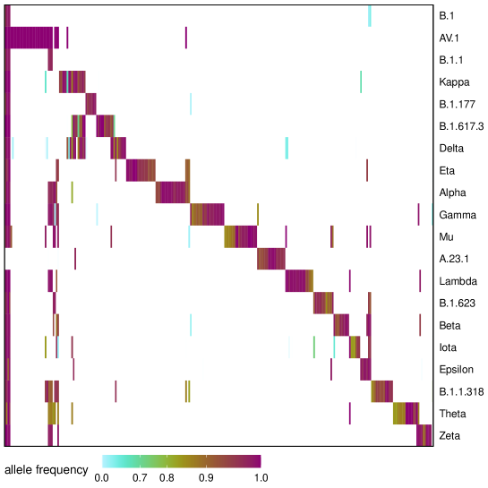
Figure 1. Polymorphism-based markers across the SARS-CoV-2 VG. The selected markers and SARS-CoV-2 VG are listed respectively as columns and rows. Cells in the heatmap are colored according to the relative frequency of each polymorphism.

4.2. Simulation study

To evaluate the performance of our method in predicting SARS-CoV-2 variant composition, we generated a synthetic dataset with 2000 simulated samples, considering non uniform coverage. As shown by Figure 2, our method performed well when applied to this data set. As expected, estimations are more accurate when based in variants found in higher relative frequencies (Figure 2A). Mean absolute errors (see (4)) were below 1% in most cases, specially for variants with relative frequencies above 25% (Figure 2B). Figure 2C shows that the mean absolute error strongly depends on sample coverage (the distribution of simulated samples coverage reflects the respective distribution on the wastewater dataset considered in Section 4.3). Finally, the adopted bootstrap estimates of standard errors can provide accurate limits for the true error, as shown in Figure 2D. Results obtained while analyzing few simulated data samples are summarized in Table 1. In particular, this table presents how results are sensitive to sample coverage and composition complexity, as well as the accuracy of adopted bootstrap approach to error estimation.

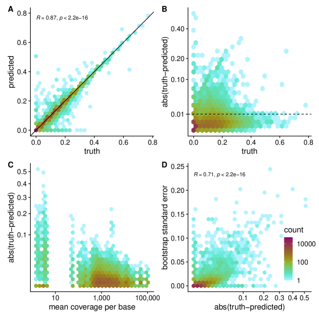
Figure 2. Performance measures for the proposed estimator. The number of points within each hexagon is reflected by its color, according to the scale on the right side. A. Model estimated proportions vs proportions actually used in simulations. B. Absolute errors in model estimations vs simulated proportions. C. Mean absolute error in model estimations vs mean sample coverage. D. Bootstrap standard error for model estimations vs absolute error.

Table 1. Results for 4 simulated samples. Mean Coverage (MC): average number of reads aligned to each considered polymorphism, that is $s^{-1}\sum_{i=1}^{s}t_{i}$. $w$: relative frequencies of each VG present in the simulation (ground truth); $\widehat{w}$: estimates of relative frequencies; $\widehat{w}_{\text{boot}}$: estimated mean of bootstrap samples; $\widehat{\text{se}}_{\text{boot}}$: bootstrap standard error estimate for $\widehat{w}$.

Sample	MC	VG	$w$	$\widehat{w}$	$\widehat{w}_{\text{boot}}$	$\widehat{\text{se}}_{\text{boot}}$
S_53	2.03	B.1	0.123	0.187	0.112	0.156
		B.1.1.318	0.137	1.4e-08	1.63e-3	0.0163
		B.1.177	0.0411	0.0756	0.0708	0.0504
		B.1.617.3	0.0548	0.0627	0.111	0.138
		B.1.621	0.0822	0.0578	0.0503	0.0385
		Delta	0.137	0.215	0.196	0.0903
		Epsilon	0.0822	0.181	0.176	0.0951
		Iota	0.0959	0.0316	0.0314	0.0319
		Lambda	0.137	0.122	0.12	0.0795
		Zeta	0.11	0.0682	0.0704	0.043
S_1583	2.94	B.1	0	0.498	0.377	0.181
		B.1.1	0.323	6.16e-08	0.0275	0.106
		B.1.1.318	0.0323	4.7e-09	5.89e-09	3.52e-09
		B.1.177	0.0323	3.86e-08	0.014	0.0866
		B.1.617.3	0.258	0.0877	0.0959	0.048
		B.1.623	0.258	0.237	0.253	0.053
		Epsilon	0	0.0849	0.125	0.125
		Gamma	0.0968	0.0916	0.0942	0.0325
S_221	732.37	Alpha	0	6.43e-4	6.71e-4	2.52e-4
		AV.1	0.0722	0.0748	0.0747	2.38e-3
		B.1	0.0928	0.107	0.108	0.0206
		B.1.1	0.0825	0.0588	0.0592	0.0203
		B.1.1.318	0.0515	0.048	0.048	2.19e-3
		B.1.177	0	1.35e-3	1.33e-3	7.32e-4
		B.1.617.3	0.103	0.105	0.106	3.39e-3
		B.1.621	0.103	0.104	0.104	2.37e-3
		B.1.623	0.103	0.104	0.104	2.59e-3
		Beta	0	1.64e-3	1.71e-3	5.7e-4
		Delta	0.103	0.101	0.101	3.34e-3
		Gamma	0.0722	0.0752	0.0752	2e-3
		Iota	0	4.11e-3	3.95e-3	1.37e-3
		Kappa	0.103	0.104	0.103	4.29e-3
		Lambda	0.0515	0.0522	0.0522	1.89e-3
		Theta	0	5.95e-4	5.87e-4	2.09e-4
		Zeta	0.0619	0.0575	0.0572	3.3e-3
S_1645	24740.78	AV.1	0.353	0.353	0.353	5.63e-4
		B.1.621	0.118	0.117	0.117	3.91e-4
		Beta	0	6.98e-4	6.54e-4	2.22e-4
		Gamma	0.118	0.118	0.118	4.31e-4
		Iota	0.118	0.116	0.116	7.6e-4
		Theta	0.294	0.294	0.294	4.67e-4

4.3. Wastewater data tests

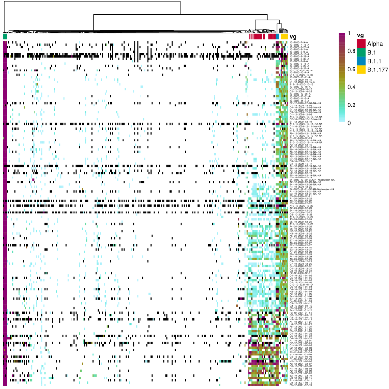
Figure 5. Polymorphisms frequencies in all wastewater samples from the Swiss dataset, ordered row-wise by collection date, with the respective markers from the 4 major VG annotated. Black cells denote no coverage in the respective sample.

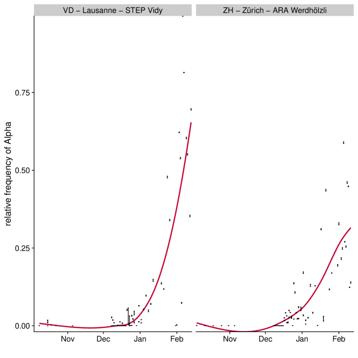
Figure 6. Graphic based on wastewater sequencing data collected over time (122 samples) in the sewage treatment plants of Lausanne and Zürich. LOESS (locally estimated scatter plot smoothing) of the Alpha VG abundance, with error bars denoting the bootstrap standard errors.

As SARS-CoV-2 variants are continuously spreading and evolving, the environment surveillance has come into play in help bringing the pandemic under control. Thus, considering that wastewater samples provide a screenshot of circulating viral lineages in the community [MBHP20], we assess the reliability and utility of our method to unveil the SARS-CoV-2 diversity from genomic sequencing data of samples collected over time in two Swiss wastewater treatment plants of Zürich (located in the canton of Zürich) and Lausanne (located in the canton of Vaud), [JDT⁺21]. Figure 5 in the Supplementary material provides an overview of the polymorphism frequencies of all markers in the pooled samples. We first recovered the relative frequencies of all SARS-CoV-2 variants (Figure 3A) from the cantons of Zürich and Vaud, previously deposited in GISAID database. Next, we compared these with the proportion of SARS-CoV-2 VGs decomposed by our method considering the viral sequencing reads obtained from the wastewater samples (Figure 3B). A loess regression, implemented in the R statistical programming language, was used to interpolate the proportion of variants between the missing time periods in the actual longitudinal data samples (Figure 3C). The evolution of the inferred relative frequencies for the Alpha variant are shown in Supplementary Figure 6. Results show the quick spread of the Alpha variant in both cantons in early December 2020 and January 2021. The trend observed in wastewater samples of both regions matches quite well the one observed in the GISAID data for COVID-19 patients.

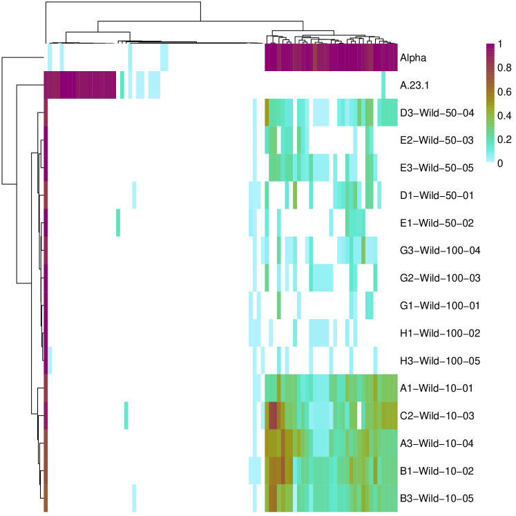
Figure 7. Heatmap result of an unsupervised hierarchical clustering of polymorphism frequencies in the dilution samples. Alpha and A.23.1 VG markers were added for comparison.

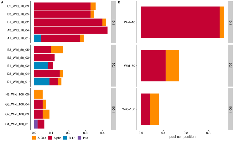
Figure 8. (A) Model predictions for each of the dilution samples replicates. (B) Model predictions after merging the replicates into a single sample.

We also explored RNA samples of SARS-CoV-2 used to assess the reproducibility of B.1.1.7 prevalence in a dilution series experiment described in [JDT⁺21]. These samples contain a mixture of wild type and Alpha/B.1.1.7 SARS-CoV-2 at ratios 10:1, 50:1 and 100:1, and each one was sequenced five times. We observed that the estimated composition is consistent with the respective dilutions (Supplementary Figure 7 and 8A). By merging the 5 replicates into a single sample, the overall coverage improves the estimates of variant composition predictions (Supplementary Figure 8B). However, we noted a small proportion of the VG A.23.1 and looking back at the marker heatmap (Supplementary Figure 7), all dilution samples reveal a mutation (S:V367F) in high frequency which is a known marker of A.23.1 [BPS⁺21]. Since the frequency of this mutation is not consistent with the dilution amounts as expected, we believe this is likely to be a sequencing artifact or contamination.

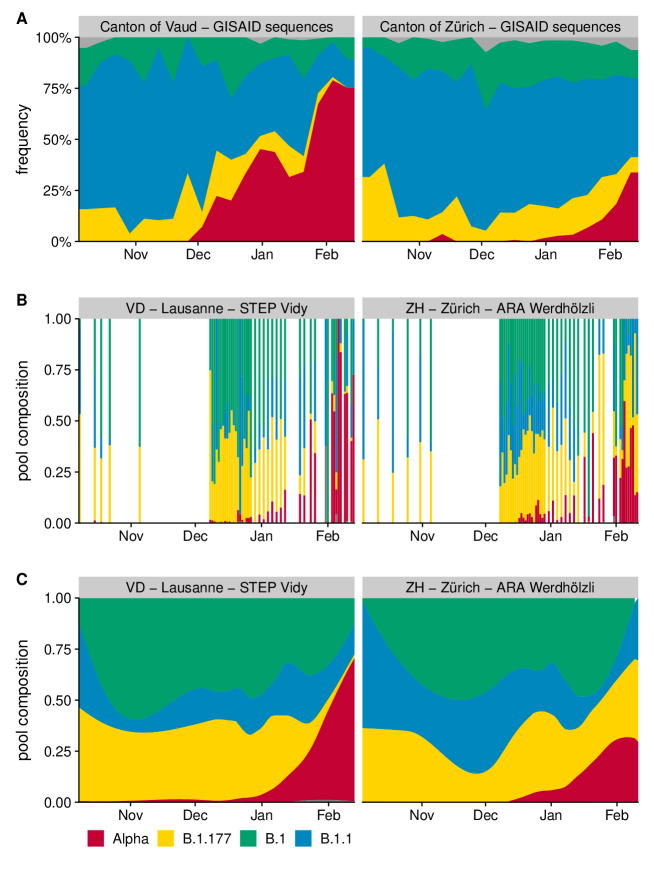
Figure 3. (A) Area plot showing the longitudinal surveillance of Alpha (red) and other SARS-CoV-2 variants based on submitted sequences from GISAID for the Cantons of Vaud (left) and Zürich (right) between October 2020 and February 2021. (B) Viral composition estimated from sequencing data of wastewater longitudinal samples collected in the sewage treatment plants of Lausanne (Canton of Vaud) and Zürich (Canton of Zurich). (C) Evolution of viral composition obtained by a loess interpolation of (B).

5. Discussion

The ability to implement continuous molecular surveillance of SARS-CoV-2 has helped to accurately detect the prevalence of viral strains. For example, measurement of SARS-CoV-2 RNA in wastewater has been shown to be a useful tool to track SARS-CoV-2 and thus may help to support public health policies. In addition to this approach, a promising genomic surveillance initiative in the city-scale monitoring encompasses the swabbing of surfaces in highly accessed locations including hospitals, airports, parks, subway and bus stations. These efforts will allow the tracking of diverse pathogens and, for COVID-19 they may accelerate the discovery of new variants and anticipate the detection of variants of clinical interest, that may lead to new waves of disease and the potential failure of some vaccines to offer long-term protection. These large-scale efforts underscore the development of novel analytical tools to identify the prevalence of viral diversity from Next-Generation Sequencing data.

This paper describes a new end-to-end approach to assess the presence of SARS-CoV-2 variant groups throughout mixed DNA samples. First, we propose a model considering the relative frequencies of polymorphic markers found in samples positive for SARS-CoV-2 genomes, likely to be derived from multiple subjects, allowing the determination of variant frequencies. Then, we systematically evaluate its performance by simulating different sequencing depths and variant relative frequencies. These dry runs highlighted the method accuracy and the sensibility of its performance to low coverage.

Next we evaluate the estimation of the relative frequency of SARS-CoV-2 lineages in public genomic sequencing data constituted by 122 wastewater samples from two cantons in Switzerland. Our results show trends in conformity with data from SARS-CoV-2-positive clinical samples, and recovered the evolution of the lineages observed in these cities. Our findings endorse the utility of viral RNA monitoring in municipal wastewater for SARS-CoV-2 infection surveillance at a population-wide level.

In addition, our pipeline uses multi-threading for efficient parallelization, and is designed on a scalable workflow engine [KR18]. The software provides a wrapper for marker calling in a bioconda environment [GDS⁺18], but it also allows the user to load their own marker selection in the variant call format (VCF). The output consists of two files, including a flat file with diversity estimation and a VCF file containing annotation of other, non-marker polymorphisms, for further analysis. The flexibility allowed by the choice of custom polymorphism-based markers, considerably widens the scope of the tools described throughout, allowing either the analysis of other viruses or regional epidemiological studies.

There are however shortcomings in our approach. The sequence coverage across the viral genome is crucial for the detection of polymorphism-based markers, and the precise determination of SARS-CoV-2 variants. Given that the viral composition assessment relies on polymorphic markers, we advise the use of a high sensitivity variant caller to detect all relevant polymorphisms. Finally, the estimation of SARS-CoV-2 variant composition may carry some uncertainty due to the stochastic nature of pool sequencing. We overcome this by considering a bootstrap approach to estimate standard errors in predictions, thus providing a measure of the reliability of each result.

In summary, we present an useful method to decompose reliable SARS-CoV-2 lineages using sequencing reads obtained from mixed samples. The effectiveness of our method on both synthetic and real data sets further demonstrates its utility for tracking SARS-CoV-2. We believe this will translate into applied tools that will aid in the environmental genomic surveillance efforts against COVID-19 outbreaks or future pandemics.

Funding

This project was funded by Fundação de Amparo à Pesquisa do Estado de São Paulo (FAPESP), grant 2021/05316-2.

Appendix

Proof of Lemma 1.

Substitution of the expression for the law of $Z_{i}$ into $L(w)$ and observing that $t_{i}=c_{i}^{r}+c_{i}^{a}$ gives

$$L(w) =\prod_{i}\prod_{j}\sum_{z_{i}\in\txcal{Z}}\frac{t_{i}!}{z_{ij}^{a}!z_{ij}^{r}!}(P_{ij}w_{j})^{z_{ij}^{a}}((1-P_{ij})w_{j})^{z_{ij}^{r}}$$

$$=\prod_{i}\sum_{z_{i}\in\txcal{Z}}\frac{t_{i}!}{c_{i}^{a}!c_{i}^{r}!}\frac{c_{i}^{a}!\prod_{j}(P_{ij}w_{j})^{z_{ij}^{a}}}{\prod_{j}z_{ij}^{a}!}\frac{c_{i}^{r}!\prod_{j}((1-P_{ij})w_{j})^{z_{ij}^{r}}}{\prod_{j}z_{ij}^{r}!}$$

$$=\prod_{i}\frac{t_{i}!}{c_{i}^{a}!c_{i}^{r}!}\bigg{(}\sum_{j}P_{ij}w_{j}\bigg{)}^{c_{i}^{a}}\bigg{(}1-\sum_{j}P_{ij}w_{j}\bigg{)}^{c_{i}^{r}}$$

$$\qquad\qquad\times\sum_{z_{i}\in\txcal{Z}}\bigg{[}\frac{c_{i}^{a}!}{\prod_{j}z_{ij}^{a}!}\bigg{(}\frac{P_{ij}w_{j}}{\sum_{j}P_{ij}w_{j}}\bigg{)}^{c_{i}^{a}}\frac{c_{i}^{r}!}{\prod_{j}z_{ij}^{r}!}\bigg{(}\frac{(1-P_{ij})w_{j}}{1-\sum_{j}P_{ij}w_{j}}\bigg{)}^{c_{i}^{r}}\bigg{]}$$

$$=\prod_{i}\frac{t_{i}!}{c_{i}^{a}!c_{i}^{r}!}\bigg{(}\sum_{j}P_{ij}w_{j}\bigg{)}^{c_{i}^{a}}\bigg{(}1-\sum_{j}P_{ij}w_{j}\bigg{)}^{c_{i}^{r}}\sum_{z_{i}^{a}\in\txcal{Z}}\frac{c_{i}^{a}!}{\prod_{j}z_{ij}^{a}!}\bigg{(}\frac{P_{ij}w_{j}}{\sum_{j}P_{ij}w_{j}}\bigg{)}^{c_{i}^{a}}$$

$$\qquad\qquad\times\sum_{z_{i}^{r}\in\txcal{Z}}\frac{c_{i}^{r}!}{\prod_{j}z_{ij}^{r}!}\bigg{(}\frac{(1-P_{ij})w_{j}}{1-\sum_{j}P_{ij}w_{j}}\bigg{)}^{c_{i}^{r}}$$

$$=\prod_{i}\frac{t_{i}!}{c_{i}^{a}!c_{i}^{r}!}\bigg{(}\sum_{j}P_{ij}w_{j}\bigg{)}^{c_{i}^{a}}\bigg{(}1-\sum_{j}P_{ij}w_{j}\bigg{)}^{c_{i}^{r}}$$

The assertion made by the lemma follows by considering the logarithm of the last expression. ∎

Proof of Lemma 2.

Throughout, let $e$ and $o$ be any two indices in $\{1,2,\ldots,v\}$. For any sample $c$ and $i\in\{1$, $2$, $\ldots$, $s\}$ define

$$Q_{i}(w)=\frac{c_{i}^{a}}{(\sum_{j=1}^{v}P_{ij}w_{j})^{2}}+\frac{c_{i}^{r}}{(1-\sum_{j=1}^{v}P_{ij}w_{j})^{2}}.$$

Straightforward computations yield

$$\frac{\partial^{2}}{\partial w_{e}^{2}}\ell(w)=-\sum_{i=1}^{s}P_{ie}^{2}Q_{i}(w)$$

and

$$\frac{\partial^{2}}{\partial w_{e}\partial w_{o}}\ell(w)=-\sum_{i=1}^{s}P_{ie}P_{io}Q_{i}(w).$$

Let $H$ be the Hessian of $\ell(w)$ with respect to $w$, namely the $v\times v$ matrix with entries $H_{eo}=\partial^{2}\ell(w)/(\partial w_{e}\partial w_{o})$. For any $u\in\mathbb{S}$ it follows that

$$u^{t}Hu =\sum_{e,o}u_{e}H_{eo}u_{o}=-\sum_{e,o}u_{e}u_{o}\sum_{i=1}^{s}P_{ie}P_{io}Q_{i}(w)$$

$$=-\sum_{i=1}^{s}Q_{i}(w)\sum_{e,o}u_{e}P_{ie}P_{io}u_{o}=-\sum_{i=1}^{s}Q_{i}(w)\bigg{(}\sum_{e}P_{ie}u_{e}\bigg{)}^{2}.$$

The fact that $Q_{i}(w)\geq 0$ for all $i$ and $w$ leads to $H$ being negative semi-definite, thus concluding the proof. ∎

Supplementary matterial

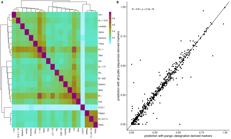
Figure 4. (A) Heatmap showing the similarities of polymorphism frequencies in SARS-CoV-2 variant groups, comparing pango-designation based markers (horizontal axis) and the equivalent markers from phylogenetic tree [TTH⁺21] (vertical axis). Similarities were calculated over polymorphisms present on both sets and measured by cosine similarity, which ranges between 0 and 1 (1 meaning a perfect match). (B) Scatter plot displaying model predictions for variant frequencies on wastewater samples, either obtained with pango-designation based markers (horizontal axis) or markers derived from all public sequences on UCSC phylogenetic tree (vertical axis).

Table 2. Variant Groups

Variant Group	Pango Lineages
A.23.1	A.23.1
AV.1	AV.1
B.1.1.318	B.1.1.318
Alpha	B.1.1.7
Beta	B.1.351, B.1.351.2, B.1.351.3
Epsilon	B.1.427, B.1.429
Eta	B.1.525
Iota	B.1.526
Kappa	B.1.617.1
Delta	B.1.617.2, AY.1, AY.2, AY.3, AY.3.1
B.1.617.3	B.1.617.3
Mu	B.1.621, B.1.621.1
B.1.623	B.1.623
Lambda	C.37
Gamma	P.1, P.1.1, P.1.2, P.1.4, P.1.6, P.1.7
Zeta	P.2
Theta	P.3
B.1.177	B.1.177
B.1.1	B.1.1
B.1	B.1

References

- [ACA+17] E. Afshinnekoo, C. Chou, N. Alexander, S. Ahsanuddin, A. N. Schuetz, and C. E. Mason. Precision Metagenomics: Rapid Metagenomic Analyses for Infectious Disease Diagnostics and Public Health Surveillance. J Biomol Tech, 28(1):40–45, 04 2017.
- [BOWI+21] I. Bar-Or, M. Weil, V. Indenbaum, E. Bucris, D. Bar-Ilan, M. Elul, N. Levi, I. Aguvaev, Z. Cohen, R. Shirazi, O. Erster, A. Sela-Brown, D. Sofer, O. Mor, E. Mendelson, and N. S. Zuckerman. Detection of SARS-CoV-2 variants by genomic analysis of wastewater samples in Israel. Sci Total Environ, 789:148002, May 2021.
- [BPS+21] D. L. Bugembe, M. V. T. Phan, I. Ssewanyana, P. Semanda, H. Nansumba, B. Dhaala, S. Nabadda, Á. N. O’Toole, A. Rambaut, P. Kaleebu, and M. Cotten. Emergence and spread of a SARS-CoV-2 lineage A variant (A.23.1) with altered spike protein in Uganda. Nat Microbiol, 6(8):1094–1101, 08 2021.
- [CBH+21] A. Christie, J. T. Brooks, L. A. Hicks, E. K. Sauber-Schatz, J. S. Yoder, and M. A. Honein. Guidance for Implementing COVID-19 Prevention Strategies in the Context of Varying Community Transmission Levels and Vaccination Coverage. MMWR Morb Mortal Wkly Rep, 70(30):1044–1047, Jul 2021.
- [D+21] D. Danko et al. A global metagenomic map of urban microbiomes and antimicrobial resistance. Cell, 184(13):3376–3393, Jun 2021.
- [DB16] Steven Diamond and Stephen Boyd. CVXPY: A Python-embedded modeling language for convex optimization. Journal of Machine Learning Research, 17(83):1–5, 2016.
- [DBP+11] M. A. DePristo, E. Banks, R. Poplin, K. V. Garimella, J. R. Maguire, C. Hartl, A. A. Philippakis, G. del Angel, M. A. Rivas, M. Hanna, A. McKenna, T. J. Fennell, A. M. Kernytsky, A. Y. Sivachenko, K. Cibulskis, S. B. Gabriel, D. Altshuler, and M. J. Daly. A framework for variation discovery and genotyping using next-generation DNA sequencing data. Nat Genet, 43(5):491–498, May 2011.
- [ET93] Bradley Efron and Robert J. Tibshirani. An introduction to the bootstrap, volume 57 of Monographs on Statistics and Applied Probability. Chapman and Hall, New York, 1993.
- [FKH+21] R. S. Fontenele, S. Kraberger, J. Hadfield, E. M. Driver, D. Bowes, L. A. Holland, T. O. C. Faleye, S. Adhikari, R. Kumar, R. Inchausti, W. K. Holmes, S. Deitrick, P. Brown, D. Duty, T. Smith, A. Bhatnagar, R. A. Yeager, R. H. Holm, N. Hoogesteijn von Reitzenstein, E. Wheeler, K. Dixon, T. Constantine, M. A. Wilson, E. S. Lim, X. Jiang, R. U. Halden, M. Scotch, and A. Varsani. High-throughput sequencing of SARS-CoV-2 in wastewater provides insights into circulating variants. medRxiv, Jan 2021.
- [GDS+18] B. Grüning, R. Dale, A. Sjödin, B. A. Chapman, J. Rowe, C. H. Tomkins-Tinch, R. Valieris, and J. Köster. Bioconda: sustainable and comprehensive software distribution for the life sciences. Nat Methods, 15(7):475–476, 07 2018.
- [GL18] J. L. Gardy and N. J. Loman. Towards a genomics-informed, real-time, global pathogen surveillance system. Nat Rev Genet, 19(1):9–20, Jan 2018.
- [HLZ+21] T. Hu, J. Li, H. Zhou, C. Li, E. C. Holmes, and W. Shi. Bioinformatics resources for SARS-CoV-2 discovery and surveillance. Brief Bioinform, 22(2):631–641, 03 2021.
- [JDT+21] Katharina Jahn, David Dreifuss, Ivan Topolsky, Anina Kull, Pravin Ganesanandamoorthy, Xavier Fernandez-Cassi, Carola Bänziger, Alexander J. Devaux, Elyse Stachler, Lea Caduff, Federica Cariti, Alex Tuñas Corzón, Lara Fuhrmann, Chaoran Chen, Kim Philipp Jablonski, Sarah Nadeau, Mirjam Feldkamp, Christian Beisel, Catharine Aquino, Tanja Stadler, Christoph Ort, Tamar Kohn, Timothy R. Julian, and Niko Beerenwinkel. Detection and surveillance of sars-cov-2 genomic variants in wastewater. medRxiv, 2021.
- [KR18] J. Köster and S. Rahmann. Snakemake-a scalable bioinformatics workflow engine. Bioinformatics, 34(20):3600, 10 2018.
- [Li18] H. Li. Minimap2: pairwise alignment for nucleotide sequences. Bioinformatics, 34(18):3094–3100, 09 2018.
- [Max21] A. Maxmen. One million coronavirus sequences: popular genome site hits mega milestone. Nature, 593(7857):21, 05 2021.
- [MBHP20] G. Medema, F. Been, L. Heijnen, and S. Petterson. Implementation of environmental surveillance for SARS-CoV-2 virus to support public health decisions: Opportunities and challenges. Curr Opin Environ Sci Health, 17:49–71, Oct 2020.
- [MHG21] D. Mercatelli, A. N. Holding, and F. M. Giorgi. Web tools to fight pandemics: the COVID-19 experience. Brief Bioinform, 22(2):690–700, 03 2021.
- [PQBC+20] D. Polo, M. Quintela-Baluja, A. Corbishley, D. L. Jones, A. C. Singer, D. W. Graham, and J. L. Romalde. Making waves: Wastewater-based epidemiology for COVID-19 - approaches and challenges for surveillance and prediction. Water Res, 186:116404, Nov 2020.
- [RAS+21] J. D. Robishaw, S. M. Alter, J. J. Solano, R. D. Shih, D. L. DeMets, D. G. Maki, and C. H. Hennekens. Genomic surveillance to combat COVID-19: challenges and opportunities. Lancet Microbe, Jul 2021.
- [RHO+20] A. Rambaut, E. C. Holmes, Á. O’Toole, V. Hill, J. T. McCrone, C. Ruis, L. du Plessis, and O. G. Pybus. A dynamic nomenclature proposal for SARS-CoV-2 lineages to assist genomic epidemiology. Nat Microbiol, 5(11):1403–1407, 11 2020.
- [SAB+21] L. C. Scott, A. Aubee, L. Babahaji, K. Vigil, S. Tims, and T. G. Aw. Targeted wastewater surveillance of SARS-CoV-2 on a university campus for COVID-19 outbreak detection and mitigation. Environ Res, 200:111374, May 2021.
- [SM17] Y. Shu and J. McCauley. GISAID: Global initiative on sharing all influenza data - from vision to reality. Euro Surveill, 22(13), 03 2017.
- [TTH+21] Y. Turakhia, B. Thornlow, A. S. Hinrichs, N. De Maio, L. Gozashti, R. Lanfear, D. Haussler, and R. Corbett-Detig. Ultrafast Sample placement on Existing tRees (UShER) enables real-time phylogenetics for the SARS-CoV-2 pandemic. Nat Genet, 53(6):809–816, 06 2021.
- [WZY+20] F. Wu, S. Zhao, B. Yu, Y. M. Chen, W. Wang, Z. G. Song, Y. Hu, Z. W. Tao, J. H. Tian, Y. Y. Pei, M. L. Yuan, Y. L. Zhang, F. H. Dai, Y. Liu, Q. M. Wang, J. J. Zheng, L. Xu, E. C. Holmes, and Y. Z. Zhang. A new coronavirus associated with human respiratory disease in China. Nature, 579(7798):265–269, 03 2020.
- [ZSZ+21] M. Zhu, J. Shen, Q. Zeng, J. W. Tan, J. Kleepbua, I. Chew, J. X. Law, S. P. Chew, A. Tangathajinda, N. Latthitham, and L. Li. Molecular Phylogenesis and Spatiotemporal Spread of SARS-CoV-2 in Southeast Asia. Front Public Health, 9:685315, 2021.