A causal fused lasso for interpretable heterogeneous treatment effects estimation
Abstract
We propose a novel method for estimating heterogeneous treatment effects based on the fused lasso. By first ordering samples based on the propensity or prognostic score, we match units from the treatment and control groups. We then run the fused lasso to obtain piecewise constant treatment effects with respect to the ordering defined by the score.
Similar to the existing methods based on discretizing the score, our methods yields interpretable subgroup effects. However, the existing methods fixed the subgroup a priori, but our causal fused lasso forms data-adaptive subgroups.
We show that the estimator consistently estimates the treatment effects conditional on the score under very general conditions on the covariates and treatment. We demonstrate the performance of our procedure using extensive experiments that show that it can outperform state-of-the-art methods.
Keywords: Nonparametric, total variation, potential
outcomes, adptivity, matching.
1 Introduction
1.1 Introduction
Causal inference focuses on the causal relationships between covariates and their outcomes, yet is deeply rooted in and advances the way we understand the world. A more precise estimation of causality empowers more reliable predictions, especially when experiments are out of the question due to high stakes of life and society, such as medical tests and personalized medicine (Zhao et al., 2017; Imbens and Rubin, 2015), and economic and public policy evaluations (Angrist and Pischke, 2008; Ding et al., 2016; Shalit et al., 2017). Our paper proposes a powerful tool for estimating heterogeneous treatment effects under nonparametric assumptions.
We adopt the potential outcomes framework (Neyman, 1923; Rubin, 1974), where each subject has an observed outcome variable caused by a treatment indicator and a set of other predictors. The main challenge in estimating heterogeneous treatment effects stems from the fact that for any given subject we only observe one realized outcome rather than both, which is also summarized as a “missing data” problem (Ding et al., 2018). To address this problem, some pioneer works largely resort to prespecified matched groups and estimate the treatment effects varying among groups, e.g. (Assmann et al., 2000; Pocock et al., 2002; Cook et al., 2004). Though effectively solving the missing data problem, earlier attempts are sensitive to the prespecified subgroups, which are identified using extensive domain knowledge or inevitably introducing arbitrariness into the causal inference. Different from those earlier works, we propose a new estimator that simultaneously identifies subgroups and estimates their treatment effects accordingly. More importantly, similar in spirit to the thought-provoking method from Abadie et al. (2018), our estimator is flexible enough to allow for non-continuous treatment effect functions.
Our estimator integrates the merits of similarity scores with the fused lasso method using a simple two-step approach. Firstly, we construct a statistic for each unit and sort observations according to it. The intuition of this step is to summarize the similarities among units using the statistics constructed. In the second step, we perform matching of units of the treatment and control groups based on the statistics generated in the first step. The differences in observed outcomes between the matched pairs guide the fused lasso method, which is a one-dimensional nonparametric regression method as introduced in Mammen et al. (1997) and Tibshirani et al. (2005), to estimate the treatment effects for different units. A key difference between our causal fused lasso approach and the usual fused lasso is that in the latter there is a given input signal and an ordering associated to it. In contrast, in causal inference there are no measurements available associated with the individual effects, which is the reason behind our two-step approach.
To be more specific, for the first step of our proposed method, we capture similarities among units using widely adopted statistics such as the propensity score (Rosenbaum and Rubin (1983, 1984)), and the prognostic score (see e.g Hansen (2008); Abadie et al. (2018)). For the former, we simply fit a parametric model such as logistic regression. For the prognostic score method, we regress the outcome on the covariates using the control group data only.
Despite being a simple and neat procedure, our method enjoys attractive properties as follows:
-
1.
From the theoretical perspective, we show that our method consistently estimates the treatment effects with minimal assumptions. These conditions include a random design of the covariates with a sub-Gaussian distribution or bounded by above and below probability density function, and bounded variation of the conditional mean of the outcome given the subgroup and the treatment assignment.
-
2.
Our estimator is computationally efficient. Its computational complexity is of order where is the number of units and the number of covariates.
-
3.
Different from many nonparametric methods, our estimator carries clear interpretations. Furthermore, as shown in our experiments, it can outperform state-of-the-art methods in estimating heterogeneous treatment effects.
1.2 Previous work
A substantial amount of work in the statistics literature has studied treatment effects in causal inference problems. A particular line of work considers the problem of testing for the existence of heterogenous treatment effects. Among these, Crump et al. (2008) developed both parametric and nonparametric tests. Lee (2009) focused on a framework for censored responses in observational studies. Sant’Anna (2020) considered a nonparametric approach that can handle right censored data.
Other authors have focused on the problem of estimating heterogenous treatment effects. A significant number of these are based on the seminal Bayesian additive regression tree models (BART) introduced Chipman et al. (2010). Roughly speaking, the idea behind BART based methods is to place a BART prior on both, the regression function of the control group and that of the treatment group. This is the case in Hill (2011); Green and Kern (2012) and Hill and Su (2013). More recently, Hahn et al. (2020) proposed a different BART based method that can deal with small effect sizes and confounding by observables. Furthermore, other Bayesian methods include the linear model prior from Heckman et al. (2014), and the Bayesian nonparametric model in Taddy et al. (2016).
In a different line of work, other authors have considered frequentist nonparametric regression methods as the basis for estimating heterogenous treatment effects. Among these, a prominent choice has become the use of regression trees. This was pioneered by Su et al. (2009) who studied an estimator exploiting the commonly used CART method from Breiman et al. (1984). More recently, Wager and Athey (2018) studied an estimator arising from the random forest method from Breiman (2001). Notably, Wager and Athey (2018) provided inferential theory for the estimated treatments, by relying on the infinitesimal jackknife Wager et al. (2014). Athey et al. (2019) took another step forward and developed a method based on generalized random forests. This resulted in a procedure that tends to be more robust in practice than the original estimator from Wager and Athey (2018).
Aside from regression tree-based methods, other machine learning approaches have been considered in the literature as a way to estimate heterogenous treatment effects. Imai et al. (2013) proposed a method that combines the hinge loss (see Wahba (2002)) with lasso regularization (Tibshirani et al., 2005). Tian et al. (2014) studied a method that can handle a large number of predictors and interactions between the treatment and covariates. Weisberg and Pontes (2015) proposed a method relying on variable selection. Taddy et al. (2016) developed Bayesian nonparametric approaches for both linear regression and tree models. Syrgkanis et al. (2019) proposed a generic approach that can build upon an arbitrary machine learning method. The resulting procedure can handle unobserved confounders if there is a valid instrument. Gao and Han (2020) studied the theoretical limitations of heterogenous treatment effects under Hölder smoothness assumptions. Künzel et al. (2019) introduced a metalernaner approach that can take advantage of any estimator, and it is probably efficient when the number of samples in one group is much larger than the other.
Finally, we highlight related work regarding the fused lasso, the nonparametric tool that we use in this paper. Also known as total variation denoising, the fused lasso first appeared in the machine learning literature (Rudin et al., 1992), and then in the statistical literature (Mammen et al., 1997). A discretized version of total variation regularization was introduced by Tibshirani et al. (2005). Since then, multiple authors have used the fused lasso for nonparametric regression in different frameworks. Tibshirani et al. (2014) proved that the fused lasso can attain minimax rates for estimation of a one-dimensional function that has bounded variation. Lin et al. (2017) and Guntuboyina et al. (2020) provided minimax results for the fused lasso when estimating piecewise constant functions. Hütter and Rigollet (2016); Chatterjee and Goswami (2019) studied the convergence rates of the fused lasso for denoising of grid graphs. Wang et al. (2016); Padilla et al. (2018) considered extensions of the fused lasso to general graphs structures. Padilla et al. (2020) proposed the fused lasso for multivariate nonparametric regression and showed adaptivity results for different levels of the regression function. Ortelli and van de Geer (2019) studied further connections between the lasso and fused lasso.
1.3 Notation
For two random variables and , we use the notation to indicate that they are independent. We write if there exist constants and such that implies that , for sequences . In addition, when and we use the notation . For a sequence of random variables , we denote if for every there exists a constant such that
Finally, for a random vector we say that is sub-Gaussian() for if
where for a random variable we have
1.4 Outline
The rest of the paper proceeds as follows. Section 2 describes the mathematical set up of the paper and presents the proposed class of estimators. Section 3 then develops theory for the corresponding estimators based on propensity and prognostic scores. Section 4 provides extensive comparisons with state of the art methods in the literature of heterogenous treatment effects. All the proofs of the theoretical results can be found in the Appendix.
2 Methodology
2.1 A predecesor estimator
Consider independent draws , where is a binary treatment indicator, is a discrete covariate, and is an outcome. Under the Stable Unit Treatment Value Assumption, we can write the observed outcome as
| (1) |
Under the unconfoundedness assumption , we can write the subgroup causal effect as
which can be identified by the joint distribution of the observed data
With large sample size, we can estimate by the sample moments:
| (2) |
where is the sample size of units with covariate value under the treatment arm .
However, the estimates ’s are well behaved only if the sample sizes ’s are large enough. With finite data, especially when is large, many ’s can be very noisy estimates of the true parameters.
When we expect that many subgroup causal effects are small or even zero in some applications, it is reasonable to shrink some ’s to zero, similar to the idea of the lasso estimator (Tibshirani, 1996). Moreover, we may also expected some subgroup causal effects are close or even identical, then it is reasonable to shrink some ’s to the same value, similar to the idea of the fused lasso (Tibshirani et al., 2005, 2014). Motivated by these considerations, it is natural to define
| (3) |
for some tuning parameter . As in Tibshirani et al. (2005) and Tibshirani et al. (2014), the second term in (3) is the fused lasso penalty to enforce a piecewise constant structure of the estimates.
While seems appealing, it requires that the covariates are univariate and categorical. Also, it requires that there is an order of the covariates under which treatment effects are piecewise constant. Both of these assumptions are usually not met in practice, as typically is a vector that can have continuous random variables. The next section proposes a general class of estimators to handle such situations.
2.2 Prognostic-based estimator
In this subsection, we focus on completely randomized experiments with , where is the covariate vector. Define as the prognostic score (Hansen, 2008). When it is known, we can discretize it to form subgroups and estimate the average causal effect within each subgroup. When it is unknown, it is common to first find the best linear approximation based on least squares
| (4) |
and then discrete the approximate prognostic score to form subgroups and estimate the subgroup effects. Abadie et al. (2018) analyzed the asymptotic properties of this method and proposed a finite-sample modification. However, these methods all assume a fixed number (often five) of subgroups based on discretizing the approximate prognostic score. We do not assume knowing the number of subgroups a priori but assume that is bounded and piecewise constant with an unknown number of pieces, or it has bounded variation; see Section 3 the precise definition. Let be the permutation such that
| (5) |
If is known and the individual causal effects are known, a natural estimator for , for , would be the solution to
| (6) |
for a tuning parameter . This is similar to the standard fused lasso for one-dimensional nonparametric regression (Tibshirani et al., 2005, 2014). The first term in (6) provides a measure of fit to the data, and the second term penalizes the total variation to ensure the restriction on the total variation.
In practice, neither or the individual treatment effects are known. We first estimate the prognostic scores as where
| (7) |
with the sequence consisting of independent copies of conditioning on . We also require that is independent of in order to establish our theory. Hence, is the estimated vector of coefficients when regressing the outcome variable on the covariates conditioning on the treatment assignment being the control group. Note that can be found in operations. Based on the estimated prognostic score, we find the permutation satisfying
| (8) |
We then match the units to impute the missing potential outcomes. Define
| (9) |
So if , then is the imputed and the imputed individual effect is ; if , then is the imputed and the imputed individual effect is . With these ingredients, we define the estimator
| (10) |
which is equivalent to
| (11) |
where is the permutation matrix associated with . The advantage of this formulation is that it is in the usual notational form of the fused lasso. Hence, it can be solved in operations by employing the algorithm from Johnson (2013) or that of Barbero and Sra (2014). Therefore, is our final estimator of the vector of subgroup treatment effects , where , for , with . Similarly, for we can estimate with where is the closest to among . A related prediction rule was used in a different context by Padilla et al. (2020).
Since by construction is piecewise constant, we can think of its different pieces as data-driven subgroups of units. These so called subgroups are estimated adaptively and do not need to be prespecified. See Figure 1 for a visual example of .
Notice that we have used a different data set for estimating the prognostic score than the one for which we estimate the treatment effects. This can be achieved in practice by sample splitting. The reason why we proceed in this way is to prevent from being correlated to .
Finally, regarding the choice of , we proceeds as in Tibshirani et al. (2012). Thus, for each value of from a list of choices, we compute the estimator in 11 and its corresponding degrees of freedom as in Tibshirani et al. (2012). Then we select the value of with the smaller Bayesian information criterion (BIC).


Example 1.
To illustrate the behavior of defined in (11) we consider a simple example. We generate with , and , from the model
| (12) | ||||
| (13) | ||||
where .
Notice that, by construction, the function is piecewise constant and depends on through a linear function. Figure 1 illustrates a plot of the vector of treatment effects . In addition, Figure 1 shows that our estimator can reasonable estimate when choosing the tuning parameter via BIC. This is surprising to an extent since the ordering that makes piecewise constant is unknown, as both the propensity score and the function are unknown.
2.3 Propensity score based estimator
Extending the method in Section 2.2 to observational studies, we define the subgroup effect as
| (14) |
where is the propensity score (Rosenbaum and Rubin, 1983). We can define an analogous estimator for based on the estimated propensity scores.
To be specific, we first fit the propensity score based on logistic regression to obtain where and
| (15) |
Again the sequence consists of independent copies of independent of . Obtain the permutation that satisfies
| (16) |
with being the associated permutation matrix. Use matching to impute the missing potential outcomes based on
| (17) |
The final estimator for becomes
| (18) |
for a tuning parameter .
One should be cautious in interpreting the prognostic score based estimator defined in (18). Specifically, (18) estimates for where
with
However, in general with as in (14). Although for all provided that . See Section 3.2 for a more detailed discussion.
Finally, the estimator based on the prognostic score (11) can be used in both randomized experiments and observational studies. However, the estimator based on the propensity score (18) only makes sense in observational studies since the true propensity score is constant in completely randomized experiments.
3 Theory
3.1 Main result for prognostic score based estimator
We start by studying the statistical behavior of the prognostic score based estimator defined in (11). Towards that end, we first introduce some assumptions needed to arrive at our first result.
Assumption 1 (Overlap).
The propensity score has support .
Assumption 2 (Surrogate prognostic score).
We write , with
, and we require that has a unique minimizer . In addition, we assume that the probability density function of is bounded by below and above. The support of is denoted as .
We notice that Assumption 2 states that the linear surrogate population prognostic score is well behaved and uniquely defined. This allows us to understand the statistical properties of defined in (7), which is potentially a misspecified maximum likelihood estimator in the language of White (1982).
Assumption 3 (Sub-Gaussian errors).
Define for , and where . Then we assume that the vector has independent coordinates that are mean zero sub-Gaussian() for some constant .
The previous assumption requires that the errors are independent, and mean zero sub-Gaussian. This condition is standard in the analysis of total variation denoising, see for instance Padilla et al. (2018). The resulting condition allows for general models such as normal, bounded distributions, and many more. In addition, Assumption 3 allows for the possibility of heteroscedastic errors.
Our next assumption has to do with behavior of the mean functions of the outcome variable, when conditioning on treatment assignment and prognostic score. We start by recalling the definition of bounded variation. For a function , we define its total variation as
| (19) |
where
We say that has bounded variation if . For a fixed , the collection
is a rich class of functions that contains important function classes, such as Lipschitz continuous functions, piecewise constant and piecewise Lipschitz functions. We refer the reader to Mammen et al. (1997); Tibshirani et al. (2014) for comprehensive studies of nonparametric regression on the class .
Assumption 4.
The functions , and for are bounded and have bounded variation. The latter means that , for , satisfy that .
Importantly, Assumption 4 allows for the possibility that functions and can have discontinuities. Our next condition imposes a relationship between the prognostic score defined in Assumption 3 and its surrogate defined in Assumption 2.
Assumption 5.
Let and be random permutations such that
and
respectively, with as defined in Assumption 2. Then we write
set for , and
and require that , where is a deterministic sequence.
Assumption 5 states that order statistics of the prognostic score at the samples are not drastically different from the order statistics of the scores based on the surrogare prognostic score. The following remark further clarifies this.
Remark 1.
Notice that can be thought as the number of units that have different relative orderings in the rankings induced by and . In addition, notice that the parameter gives an upper bound on the entries of the vector . In fact, can be thought as an version of the Kendall-Tau distance between the permutations and . Such Kendall-Tau distance is given as (see Kumar and Vassilvitskii (2010) for an overview). Readers can also consider cases in which and induce the same ordering. In such cases, can be taken as zero.
Our next assumption is a condition on the covariates.
Assumption 6.
The random vectors are independent copies of which has support , for some fixed points . In addition, the following holds:
-
•
The probability density function of , , is bounded. This amounts to
for some positive constants and .
-
•
There exist such that
(20) where and are the minimum and maximum eigenvalue functions.
We emphasize that the first condition in Assumption 6 is standard in nonparametric regression, see Padilla et al. (2020). It is slightly more general than assuming that the covariates are uniformly drawn in as in the nonparametric regression models in Györfi et al. (2006), and the heterogenous treatment effect setting from Wager and Athey (2018).
As for (20), this condition ensures that the design matrix is well behaved. In particular, it immediately holds if .
With these assumptions, we are now ready to state our first result regarding the estimation of , with the prognostic score defined in Assumption 3.
Theorem 1.
We notice that is a strong assumption that might not hold in observational studies, however it might be reasonable in completely randomized trials.
On another note, Theorem 1 shows that we can consistently estimate the subgroup treatment effects provided that
and the assumptions of Theorem 1 hold. If we ignore the logarithmic factors, the dependence on , and assume that , we obtain a rate of as an upper bound on the mean squared error of our proposed estimator. This rate is worst that the rate in one-dimensional nonparametric regression with the fused lasso, which in the class of bounded variation is . However, the main difference from such setting to ours, has to do with the fact that our design depends on the ’s which need to be estimated. We do not claim that our procedure is minimax, in fact we conjecture that it is not. Nevertheless, out method is computationally efficient and consistent, making it attractive in practice as we will see in Section 4.
We conclude this section with a remark that can be thought as a straightforward generalization of Theorem 1.
Remark 2.
Notice that the rate does not depend on the dimension of the covariates as it is the case of other nonparametric estimators, see Gao and Han (2020). In fact our results are not directly comparable with Gao and Han (2020) as the authors there consider different classes of functions. A main driver behind the rate is Assumption 4. If instead is allowed to grow, then the upper bound in Theorem 1 should be inflated by a factor . Hence, similarly to the discussion above this would lead to the rate .
3.2 Main result for propensity score based estimator
We now study the statistical properties of the estimator defined in Section 2.3. Since the assumptions required to arrive at our main result here are similar to those in Section 3.1, here we only present the conclusion of our result and the assumptions are given in Section B.
Theorem 2.
Importantly, Theorem 3 implies that the estimator defined in (18) can consistently estimate the subrgroup treatment effects under general conditions. One of such conditions is that , which in the language of Rosenbaum and Rubin (1983) means that treatment is strongly ignorable given . As Theorem 3 in Rosenbaum and Rubin (1983) showed, holds under overlapping (Assumption 1) and unconfoundedness which can be wrriten as . When these conditions are violated, Theorem 3 shows that can still approximate under Assumptions 1, and 7–11.
4 Experiments
We will no validate with experiments the proposed methods in this paper. Throughout, we will refer to the procedure in Section 2.2 as causal fused lasso 1 (CFL1), and the corresponding in Section 2.3 as causal fused lasso (CFL2). For both of our estimators we select the tuning parameter using BIC as discussed in Section 2.2. As for competitors, we will benchmark against the causal random forests-Procedure 1 (denoted WA1) and Procedure 2 (denoted WA2)–of Wager and Athey (2018), the robust generalized random forests (denoted GRF) in section 6.2 of Athey et al. (2019), and the estimator from Abadie et al. (2018) (ACW).
4.1 Comparisons with Wager and Athey (2018), and Athey et al. (2019)
To compare against Wager and Athey (2018), and Athey et al. (2019), we use four generative models as described below. For each model, we consider varying values of and . For each combination of these parameters, we generate a data set according to the corresponding generative model. Based on 50 Monte Carlo trials, we use the mean squared error as a measure of performance. This is defined as
where , and is a given estimator.
A for generative models, we consider four scenarios. The details as described in Section E. The first two scenarios come from Wager and Athey (2018) and both consists of for all . In Scenario 3 we have that for all , where for a fixed , and with the cumulative distiribution function of the standard normal distribution. Furthermore, Scenario 4 is the model described in (12).
With these generative models, the results of our experiments are shown in Table 1. There, we can see that for Scenario 1 the best methods are our proposed estimators, which is reasonable since the treatment effect is zero across units. In Scenario 2, we do not compare CFL2 since such method is not suitable for experimental designs where the propensity score takes on a constant value. The best method in this case is GRF. In Scenario 3, we see that CFL2 outperforms the competitors. Notice that in Scenario 3 the treatment effect is a function of the propensity score, where the propensity score belongs to the family of probit models. This does not seem to be a problem for our estimator which provides accurate estimation despite relying on logistic regression in the first stage. Finally, in Scenario 4, we see that CFL1 outperforms the competitors. Again, since the propensity score is constant, we do not benchmark CFL2.
| Scenario | WA1 | WA2 | GRF | CFL1 | CFL2 | ||
|---|---|---|---|---|---|---|---|
| 1 | 800 | 2 | 0.045 | 0.012 | 0.013 | 0.004 | 0.011 |
| 1 | 1600 | 2 | 0.029 | 0.010 | 0.011 | 0.003 | 0.004 |
| 1 | 800 | 10 | 0.067 | 0.007 | 0.010 | 0.005 | 0.016 |
| 1 | 1600 | 10 | 0.068 | 0.003 | 0.006 | 0.003 | 0.005 |
| 2 | 800 | 2 | 0.495 | 0.264 | 0.152 | 0.704 | * |
| 2 | 1600 | 2 | 0.199 | 0.164 | 0.063 | 0.567 | * |
| 2 | 800 | 10 | 0.773 | 0.794 | 0.565 | 0.979 | * |
| 2 | 1600 | 10 | 0.534 | 0.723 | 0.350 | 0.978 | * |
| 3 | 800 | 2 | 0.226 | 0.143 | 0.143 | 0.181 | 0.074 |
| 3 | 1600 | 2 | 0.164 | 0.106 | 0.106 | 0.136 | 0.051 |
| 3 | 800 | 10 | 0.550 | 0.362 | 0.408 | 0.412 | 0.146 |
| 3 | 1600 | 10 | 0.499 | 0.316 | 0.359 | 0.293 | 0.109 |
| 4 | 800 | 2 | 4.923 | 2.922 | 1.788 | 0.301 | * |
| 4 | 1600 | 2 | 3.228 | 2.049 | 0.771 | 0.183 | * |
| 4 | 800 | 10 | 6.528 | 5.796 | 3.261 | 0.450 | * |
| 4 | 1600 | 10 | 6.146 | 5.322 | 1.291 | 0.277 | * |
| Scenario | CFL2 | ACW | ||
|---|---|---|---|---|
| 1 | 3764 | 79 | 0.044 | 0.016 |
| 2 | 2530 | 18 | 1094503 | 3554551 |
| 3 | 4000 | 10 | 0.081 | 0.471 |
| 4 | 4000 | 10 | 0.077 | 0.137 |
4.2 Comparisons with Abadie et al. (2018)
To compare against Abadie et al. (2018) we proceed in a similarly way to our experiments in Section 4.1. Here, and are as before the number samples and the environment dimension, respectively, of the training data. Next we discuss the different scenarios that we consider.
Scenario 1. As a first scenario we use the setting of the National JTPA Study used in Abadie et al. (2018). This consists of a National JTPA Study evaluating an employment and training program commissioned by the U.S. Department of Labor in the late 1980s. Other authors that have also analyzed this data include Orr (1996) and Bloom et al. (1997).
In the JTPA study, based on a randomized assignment, subjects were a assigned into one of two groups. In the treatment group the subjects had access to JTPA services that included one of three possibilities: on-the-job training/job search assistance, classroom training, and other services. In contrast, subjects in the control group were not given access to the JTPA services. The raw data consists of 2530 units , 1681 of which are treated observations and 849 are untreated observations. With these measurements, we generate simulated data as in Abadie et al. (2018) where the treatment effect is zero across all units. The details are given in Section F.1.
Scenario 2. For our second model we also considered an example used in Abadie et al. (2018). Specifically, we use the Project STAR class-size study, see for instance Krueger (1999). In this data, 3,764 students who entered the study in kindergarten were assigned to small classes or to regular-size classes (without a teacher’s aide). The outcome variable is standardized end-of-the-year kindergarten math test scores. As for covariates, some of these include race, eligibility for the free lunch program, and school attended. With the original data we proceed as in Abadie et al. (2018) and simulate data in a setting where the treatment effects are all zero. The details are given in F.2.
Scenario 3. This scenario also comes from Abadie et al. (2018). Setting and the data is generated as: , and , where . Moreover, the treatment indicators for the simulations are such that . Clearly, the vector of treatment effects satisfies .

Scenario 4. For our final model we set , , and generate data as
where with if , and otherwise. Notice that in this case the treatment effect for unit is .
With the four scenarios from above, we compare CFL1, our proposed prognostic score based estimator, against the method from Abadie et al. (2018). The results in Table 2 and Figure LABEL:fig3 show that in two of the three scenarios where there the treatment effect is zero CFL1 clearly outperforms the method from Abadie et al. (2018). Furthermore, in Scenario 4, which has a nonconstant treatment effect function, our method also outperforms that from Abadie et al. (2018). These findings are not surprising given that CFL1 adaptively chooses the subgroups whereas Abadie et al. (2018) is based on an ad hoc way of doing that.
4.3 National Supported Work data
4.4 Randomized example
To illustrate the behavior of our estimators, we use the data from LaLonde (1986); Dehejia and Wahba (1999, 2002). This dataset consists of a 445 sub-sample from the National Supported Work Demonstration (NSW). The NSW was a program implemented in the mid-1970s in which the treatment group consisted of randomly selected subjects to gain 12 to 18 months of work experience and 260 subjects in a control group. The response variable is the post-study earnings in 1978. The predictor variables include age, education, indicator of Black and Hispanic for race, marital status, high-school degree indicator, earnings in 1974, and earnings in 1975.
To construct our estimator, we first estimate the prognostic score using the data from the control group and running a linear regression model. With the prognostic scores, we then compute an ordering and run the fused lasso leading to our CFL2 estimator. This is depicted in Figure 2. There, we also see the estimates based on the method ACW from Abadie et al. (2018). We can see that both CFL2 and ACW estimate small positive treatment effects, which might be expected given the nature of the NSW program.
4.5 Observational example
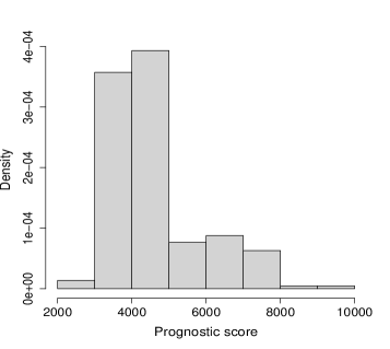
For our second example based on the NSW data, we combine the 185 observations in the treatment group of the data from Section 4.4 with the largest of the six observational control groups constructed by Lalonde111Dataset is available here http://users.nber.org/ rdehejia/nswdata2.html. This results in a total of 16177 samples. Due to the observational nature of the dataset, we run our propensity score based estimator from Section 2.3 by only estimating treatment effects on the treated. Thus, our estimator is the one described in Corollary 4 which we denote as CFL2. We can see in Figure 3 that CFL2 estimates a constant positive treatment effect which is consistent with our finding in Section 4.4.
4.6 National Health and Nutrition Examination Survey
In our final example we use data from the 2007–2008 National Health and Nutrition Examination Survey (NHANES). The data consist of 2330 children and their participations in the National School Lunch or the School Breakfast programs in order to assess the effectiveness of such meal programs in increasing body mass index (BMI). In the study 1284 randomly selected children participated in the meal programs while 1046 did not. The predictor variables are age, gender, age of adult respondent, and categorical variables such as Black race, Hispanic race, whether the family of the child is above 200% of the federal poverty level, participation in Special Supplemental Nutrition program, Participation in food stamp program, childhood food security, any type of insurance, and gender of the adult respondent.
Similarly as before, we run our propensity score based estimator (CFL2) and show the results in Figure 3. We can see that the sign of estimated treatment effects varies depending on the value of the propensity score. The latter was estimated by a logistic regression. Our findings for the treatment effects coincide with several authors who found positive and negative average treatment effects as discussed in Chan et al. (2016).
5 Acknowledgment
We are very thankful to Peng Ding for constructive and stimulating discussions.
Appendix A Possible extensions
A natural extension of the estimators described in Sections 2.2 and 2.3 is to consider the case where the number of covariates can be large, perhaps , but only a small number of them plays a role in the prognostic score (propensity score). In the case of the prognostic score based estimator, a natural extension is to estimate with lasso regression (Tibshirani, 1996). The resulting procedure would be the same as in Section 2.2, except that we would define where
for a tuning parameter . Similarly, we can modify the propensity score estimator, replacing by -regularized logistic regression in the spirit of Ravikumar et al. (2010).
A simpler modification of the estimators from Sections 2.2–2.3 can be obtained by adding a sparsity penalty in the objective function. This is similar to the definition of the fused lasso in Tibshirani et al. (2005). The resulting estimator would be reasonable if there is a believe that most of the treatment effects are zero. It would basically amount to apply soft-thresholding to the estimators from (11)–(18), see for instance Wang et al. (2016).
Appendix B Main result for propensity score based estimator
We now study the statistical properties of the estimator defined in Section 2.3. As in Section 3.2 we start by stating required assumptions.
Assumption 7 (Sub-Gaussian errors).
Define with as in Assumption 1. Then the vector has independent coordinates that are mean zero sub-Gaussian.
Assumption 7 is the parallel of Assumption 3 when we replace the prognostic score with the propensity score.
Assumption 8.
The functions , and for are bounded and have bounded variation.
As for the distribution of the covariates, we allow for more generality than in Section 3.2. Specifically, we allow for general multivariate sub-Gaussian distributions. The reason why we loosen up, compared to the first part of Assumption 6, is that the propensity score is bounded making the analysis more transparent.
Assumption 9 (Distribution of covariates).
The random vector is centered () sub-Gaussian(C).
We refer the reader to Vershynin (2010) which contains important concentrations results regarding multivariate sub-Gaussian distributions. We exploit some of those in our proofs.
Assumption 10.
The propensity score staisfies for some . Furthermore is a continuous random variable with pdf bounded by above ( for some positive constant ), and there exist constants and such that
| (24) |
for all , where is a constant, and (24) holds for all in the support of .
Assumption 11 (Dependency condition).
Let and be the minimum and maximum eigenvalue functions, respectively. Then, we assume that there exist positive and such that
and
with with as in Assumption 10, and where is a large enough constant. We also require that
| (25) |
for a large enough constant .
Assumption 11 is basically the Dependency condition in the analysis of high-dimensional logistic regression from Ravikumar et al. (2010). As the authors there assert, this condition prevents the covariates from becoming overly dependent.
We are now in position to present the main result regarding our propensity scored based estimator.
Theorem 3.
Importantly, Theorem 3 implies that the estimator defined in (18) can consistently estimate the subrgroup treatment effects under general conditions. One of such conditions is that , which in the language of Rosenbaum and Rubin (1983) means that treatment is strongly ignorable given . As Theorem 3 in Rosenbaum and Rubin (1983) showed, holds under overlapping (Assumption 1) and unconfoundedness which can be wrriten as . When these conditions are violated, Theorem 3 shows that can still approximate under Assumptions 1, and 7–11.
Furthermore, as in Remark 2, Theorem 3 can be relaxed. Specifically, we can replace Assumption 8 with
Then the upper bound in Theorem 3 needs to be inflated by .
We conclude this section with immediate consequence of the proof of Theorem 3 concerning heterogenous treatment effects of the treated units.
Corollary 4 (Treatment effects of the treated).
Suppose that the conditions of Theorem 3 for (27) to hold are met. Let be the propensity score estimator from Section 2.3 with a slight modification. After the matching is done and the signal is calcluated, we only run the the fused lasso estimator, with the ordering based on the estimated propensity score, on the treated units. Then
| (28) |
where for . If in addition , then (28) holds replacing with for .
Appendix C Proof of Theorem 3
Throughout this section we write
we also write
C.1 Total variation auxiliary lemmas
Lemma 5.
The estimator defined in (18) satisfies
Proof.
We beging by introducing some notation. For a vector , a vector is defined as
To proceed with first condition on and . Then by the definition of and the KKT conditions, we have that
| (29) |
where is the Hadamard product. Next, notice that (29) implies that
The claim then follows since , by Sub-Gaussian tail inequality, and integrating over and . ∎
Proof.
Let , we have
and
On the other hand, since are independent and identically distributed, we have that
Therefore, by Chernoff’s inequality and union bound,
and so the claim follows by the sub-Gaussian tail inequality.
∎
Lemma 7.
Proof.
Let , the row space of . Also write and for the orthogonal projection matrices onto and its orthogonal complement , respectively. Then let
where , for . Hence, , see Proof of Theorem 3 in Wang et al. (2016). Therefore,
| (33) |
However, by the sub-Gaussian tail inequality,
| (34) |
Therefore, combining (33), (34), (31) and Lemma 6,
Next, we proceed to bound . Notice that by the optimality of
| (35) |
where
for .
Then by Hölder’s inequality, Lemma 5 and (5), there exists a constant such that, with probability approaching one,
| (36) |
where
for some positive constant .
Next, suppose that . Then, due to our choice of , (35), and (36), there exists such that
| (37) |
with probability approaching one.
On the contrary, if , then (35) and (36) imply
| (38) |
Next, we proceed to bound the first term in the right hand size of the previous inequality. Towards that end, with the notation from the proof of Lemma 6, we exploit the argument in the proof of Lemma 9 from Wang et al. (2016). First, by Lemma 9, Theorem 10, and Corollary 12 from Wang et al. (2016), we have that
| (39) |
which follows due to the independence and sub-Gaussian assumption of the errors .
On the other hand, conditioning on and , we define the random vectors , constructed as follows. First, let
Then
and
And for , we iteratively construct
Notice that, by construction, the components of each are independent and subGaussian(). Hence, by triangle inequality,
Then as in the proof of Theorem 10 in Wang et al. (2016), which exploits Lemma 3.5 from Van de Geer (1990), we have that
for some constant , and for any constant , where is a fixed constant.
Therefore, by a union bound,
| (40) |
Hence, combining (39) with (40), integrating over and , and proceeding as in the proof of Lemma 6, we arrive at
| (41) |
where
Next, we notice that due to (38) , (41), the proof of Lemma 9 in Wang et al. (2016), we have that
| (42) |
and
Hence, combining (37) and (42), we obtain that
and the claim follows.
∎
C.2 Propensity score auxiliary lemmas
Lemma 8.
Proof.
Lemma 9.
Proof.
Proceeding as in the proof of Lemma 5 in Ravikumar et al. (2010), we obtain that
where denotes the spectral norm and with
To bound the quantity we let with , and notice that
and by Proposition 5.16 in Vershynin (2010)
for all , and for an absolute constant . Hence, taking , and with the same entropy based argument from the proof of Lemma 5 in Wang et al. (2017), we arrive at
Finally,
and the proof concludes with the same argument from above.
∎
Lemma 10.
Proof.
For let
Clearly, , and where . Let
| (45) |
We proceed to show that for all , which implies, by convexity, that . Towards that end, notice that, by Taylor’s theorem, we have
for some . Also,
Hence, by Lemma 8 and a union bound,
| (46) |
with probability at least .
Furthermore,
Also,
| (47) |
where
Now for , with , we have
| (48) |
with probability approaching one, and where is a constant. Here, we have used the fact the random variables are sub-Gaussian, and the second claim in Lemma 9. Therefore, with probability approaching one,
where the first inequality follows from (46)– (48), the second from (45) and (25), and the third since
∎
Lemma 11.
C.3 Lemma combining both stages
Lemma 12.
There exists a positive constant such that the event
holds with probability approaching one.
Proof.
Then for each define
where for a positive constant to be chosen later.
Then by Assumption 10,
Hence,
Therefore, by a union bound, and Chernoff’s inequality,
| (51) |
provide that is chosen large enough.
On the other hand, by (50), we have
-
•
If , then .
-
•
If , then .
Lemma 13.
With the notation from before,
and
Proof.
Suppose that the event
| (52) |
holds for some positive constant , see Lemma 12.
Then
and the claim follows.
∎
Lemma 14.
There exists a positive constant such that the event
| (53) |
happens with probability approaching one.
Proof.
Let be a constant to be chosen later. Fix and define
and .
Then we have that
Hence, by union bound,
and so we set . The claim follows by Assumption 10 and the argument in the proof of Proposition 30 in Von Luxburg et al. (2014) implying that, with high probability, the distance of of each to its nearest neighbor is of order for .
∎
Lemma 15.
For any let
Then, for some constant ,
with probability approaching one.
Proof.
First, assume that the event (50) holds. Next, by Lemma 14, with high probability, for all there exits such that and . Under such event,
where the second inequality follows from the definition of , the third and fourth from Lemma 11, and the last from the construction of . Therefore,
and the claim follows in the same way that we bounded the counts in the proof of Lemma 12. ∎
Lemma 16.
With the notation from before,
for .
Proof.
By Lemma 15 and the triangle inequality, we have that, with probability approaching one,
and the claim follows.
∎
C.4 Proof of Theorem 3
Appendix D Proof of Theorem 1
D.1 Notation
Throughout this section we define the function as
and set
Furthermore, we consider the orderings , , and satisfying
| (54) |
| (55) |
and
| (56) |
D.2 Auxiliary lemmas
Proof.
First notice that by the optmiality of we have that
Hence,
Furthermore, defining , we have
| (57) |
where the first inequality follows by Hölder’s inequality, and the second by the relation between and norms.
However, by Assumption 3, it follows that
holds with probability at least . Hence, by Assumption 6, (57), and Hoeffding’s inequality
with proability .
∎
Lemma 18.
For any let
Then, for some constant ,
with probability approaching one.
Proof.
We define the function
and observe that , and where . Let
for some , and take such that . Then, with probability approaching one, by Lemma 17 and the proof of Lemma 9, we have that
for some constant , and where the last inequality follows from the choice of with a large enough .
Therefore,
| (58) |
with probability approaching one. Furthermore,
| (59) |
and the conclusion follows from (58) and the fact the have compact support. ∎
D.3 Proof of Theorem 1
The theorem follows as a Theorem 7, proceeding as in the proof of Theorem 3 by using the lemmas below.
Lemma 20.
Lemma 21.
Proof.
By Lemma 20 and the triangle inequality, we have that, with probability approaching one,
Furthermore,
| (60) |
However, if , then is between and , , and . Therefore, either or . Hence,
where the last inequality follows from Assumption 5. The proof for proceeds with the same argument.
∎
Lemma 22.
For any let
Then, for some constant ,
with probability approaching one.
Proof.
This follows as the proof of Lemma 15. ∎
Lemma 23.
Appendix E Details for comparisons with Wager and Athey (2018), and Athey et al. (2019)
Scenario 1. This is the first model considered in Wager and Athey (2018) (see Equation 27 there). The data satisfies
where , and is -density with shape parameters and . Notice that in this case for all .
Scenario 2. Our second scenario also comes from Wager and Athey (2018) (see Equation 28 there).
Hence, once again for all .
Scenario 3. Here we generate the measurements as
where with if , and otherwise. Furthermore, denotes the cumulative distiribution function of the standard normal distribution. Clearly, in this case for all .
Scenario 4. This is the model described in (12).
Appendix F Details of comparisons with Abadie et al. (2018)
F.1 National JTPA Study
We follow the experimental setting in Abadie et al. (2018). Specifically, let the JTPA measurements be , where corresponds to the outcome (earnings), to the covariates, and to the treatment indicator. Then, to generate simulated outcomes, construct a parameter as in Abadie et al. (2018):
where .
Furthermore, the variance of the errors is computed as:
A third parameter of interest is:
the result of fitting a logistic regression model to predict whether a unit in the experiment’s control group will have positive earnings.
Next, simulation data is generated as:
Here, the treatment effect is zero. Furthermore, the treatment indicators for the simulations are such that for the training set, and for the test set.
F.2 Project STAR
With the observations for this study, where is the outcome variable, the vector of covariates, and the treatment assignment, we generate data following Abadie et al. (2018). Thus, measurements arise from the model
where
and the variance for the errors is computed as:
Finally, in this scenario, the treatment indicators for the simulations are such that .
Appendix G National Supported Work data
References
- Abadie et al. (2018) Abadie, A., Chingos, M. M. and West, M. R. (2018). Endogenous stratification in randomized experiments. Review of Economics and Statistics 100 567–580.
- Angrist and Pischke (2008) Angrist, J. D. and Pischke, J.-S. (2008). Mostly harmless econometrics: An empiricist’s companion. Princeton university press.
- Assmann et al. (2000) Assmann, S. F., Pocock, S. J., Enos, L. E. and Kasten, L. E. (2000). Subgroup analysis and other (mis) uses of baseline data in clinical trials. The Lancet 355 1064–1069.
- Athey et al. (2019) Athey, S., Tibshirani, J., Wager, S. et al. (2019). Generalized random forests. The Annals of Statistics 47 1148–1178.
- Barbero and Sra (2014) Barbero, A. and Sra, S. (2014). Modular proximal optimization for multidimensional total-variation regularization. arXiv preprint arXiv:1411.0589 .
- Bloom et al. (1997) Bloom, H. S., Orr, L. L., Bell, S. H., Cave, G., Doolittle, F., Lin, W. and Bos, J. M. (1997). The benefits and costs of jtpa title ii-a programs: Key findings from the national job training partnership act study. Journal of human resources 549–576.
- Boucheron et al. (2013) Boucheron, S., Lugosi, G. and Massart, P. (2013). Concentration inequalities: A nonasymptotic theory of independence. Oxford university press.
- Breiman (2001) Breiman, L. (2001). Random forests. Machine learning 45 5–32.
- Breiman et al. (1984) Breiman, L., Friedman, J., Olshen, R. and Stone, C. (1984). Classification and regression trees (cart). Wadsworth, Monterey, CA, USA .
- Chan et al. (2016) Chan, K. C. G., Yam, S. C. P. and Zhang, Z. (2016). Globally efficient non-parametric inference of average treatment effects by empirical balancing calibration weighting. Journal of the Royal Statistical Society. Series B, Statistical methodology 78 673.
- Chatterjee and Goswami (2019) Chatterjee, S. and Goswami, S. (2019). New risk bounds for 2d total variation denoising. arXiv preprint arXiv:1902.01215 .
- Chipman et al. (2010) Chipman, H. A., George, E. I., McCulloch, R. E. et al. (2010). Bart: Bayesian additive regression trees. The Annals of Applied Statistics 4 266–298.
- Cook et al. (2004) Cook, D. I., Gebski, V. J. and Keech, A. C. (2004). Subgroup analysis in clinical trials. Medical Journal of Australia 180 289.
- Crump et al. (2008) Crump, R. K., Hotz, V. J., Imbens, G. W. and Mitnik, O. A. (2008). Nonparametric tests for treatment effect heterogeneity. The Review of Economics and Statistics 90 389–405.
- Dehejia and Wahba (1999) Dehejia, R. H. and Wahba, S. (1999). Causal effects in nonexperimental studies: Reevaluating the evaluation of training programs. Journal of the American statistical Association 94 1053–1062.
- Dehejia and Wahba (2002) Dehejia, R. H. and Wahba, S. (2002). Propensity score-matching methods for nonexperimental causal studies. Review of Economics and statistics 84 151–161.
- Ding et al. (2016) Ding, P., Feller, A. and Miratrix, L. (2016). Randomization inference for treatment effect variation. Journal of the Royal Statistical Society: Series B (Statistical Methodology) 78 655–671.
- Ding et al. (2018) Ding, P., Li, F. et al. (2018). Causal inference: A missing data perspective. Statistical Science 33 214–237.
- Gao and Han (2020) Gao, Z. and Han, Y. (2020). Minimax optimal nonparametric estimation of heterogeneous treatment effects. arXiv preprint arXiv:2002.06471 .
- Green and Kern (2012) Green, D. P. and Kern, H. L. (2012). Modeling heterogeneous treatment effects in survey experiments with bayesian additive regression trees. Public opinion quarterly 76 491–511.
- Guntuboyina et al. (2020) Guntuboyina, A., Lieu, D., Chatterjee, S., Sen, B. et al. (2020). Adaptive risk bounds in univariate total variation denoising and trend filtering. The Annals of Statistics 48 205–229.
- Györfi et al. (2006) Györfi, L., Kohler, M., Krzyzak, A. and Walk, H. (2006). A distribution-free theory of nonparametric regression. Springer Science & Business Media.
- Hahn et al. (2020) Hahn, P. R., Murray, J. S., Carvalho, C. M. et al. (2020). Bayesian regression tree models for causal inference: regularization, confounding, and heterogeneous effects. Bayesian Analysis .
- Hansen (2008) Hansen, B. B. (2008). The prognostic analogue of the propensity score. Biometrika 95 481–488.
- Heckman et al. (2014) Heckman, J. J., Lopes, H. F. and Piatek, R. (2014). Treatment effects: A bayesian perspective. Econometric reviews 33 36–67.
- Hill and Su (2013) Hill, J. and Su, Y.-S. (2013). Assessing lack of common support in causal inference using bayesian nonparametrics: Implications for evaluating the effect of breastfeeding on children’s cognitive outcomes. The Annals of Applied Statistics 1386–1420.
- Hill (2011) Hill, J. L. (2011). Bayesian nonparametric modeling for causal inference. Journal of Computational and Graphical Statistics 20 217–240.
- Hütter and Rigollet (2016) Hütter, J.-C. and Rigollet, P. (2016). Optimal rates for total variation denoising. In Conference on Learning Theory.
- Imai et al. (2013) Imai, K., Ratkovic, M. et al. (2013). Estimating treatment effect heterogeneity in randomized program evaluation. The Annals of Applied Statistics 7 443–470.
- Imbens and Rubin (2015) Imbens, G. W. and Rubin, D. B. (2015). Causal inference in statistics, social, and biomedical sciences. Cambridge University Press.
- Johnson (2013) Johnson, N. A. (2013). A dynamic programming algorithm for the fused lasso and l 0-segmentation. Journal of Computational and Graphical Statistics 22 246–260.
- Krueger (1999) Krueger, A. B. (1999). Experimental estimates of education production functions. The quarterly journal of economics 114 497–532.
- Kumar and Vassilvitskii (2010) Kumar, R. and Vassilvitskii, S. (2010). Generalized distances between rankings. In Proceedings of the 19th international conference on World wide web.
- Künzel et al. (2019) Künzel, S. R., Sekhon, J. S., Bickel, P. J. and Yu, B. (2019). Metalearners for estimating heterogeneous treatment effects using machine learning. Proceedings of the national academy of sciences 116 4156–4165.
- LaLonde (1986) LaLonde, R. J. (1986). Evaluating the econometric evaluations of training programs with experimental data. The American economic review 604–620.
- Lee (2009) Lee, M.-j. (2009). Non-parametric tests for distributional treatment effect for randomly censored responses. Journal of the Royal Statistical Society: Series B (Statistical Methodology) 71 243–264.
- Lin et al. (2017) Lin, K., Sharpnack, J. L., Rinaldo, A. and Tibshirani, R. J. (2017). A sharp error analysis for the fused lasso, with application to approximate changepoint screening. In Advances in Neural Information Processing Systems.
- Mammen et al. (1997) Mammen, E., van de Geer, S. et al. (1997). Locally adaptive regression splines. The Annals of Statistics 25 387–413.
- Neyman (1923) Neyman, J. (1923). Sur les applications de la théorie des probabilités aux experiences agricoles: Essai des principes. Roczniki Nauk Rolniczych 10 1–51.
- Orr (1996) Orr, L. L. (1996). Does training for the disadvantaged work?: Evidence from the National JTPA study. The Urban Insitute.
- Ortelli and van de Geer (2019) Ortelli, F. and van de Geer, S. (2019). Synthesis and analysis in total variation regularization. arXiv preprint arXiv:1901.06418 .
- Padilla et al. (2020) Padilla, O. H. M., Sharpnack, J., Chen, Y. and Witten, D. M. (2020). Adaptive non-parametric regression with the -nn fused lasso. Biometrika .
- Padilla et al. (2018) Padilla, O. H. M., Sharpnack, J. and Scott, J. G. (2018). The dfs fused lasso: Linear-time denoising over general graphs. The Journal of Machine Learning Research 18 6410–6445.
- Pocock et al. (2002) Pocock, S. J., Assmann, S. E., Enos, L. E. and Kasten, L. E. (2002). Subgroup analysis, covariate adjustment and baseline comparisons in clinical trial reporting: current practiceand problems. Statistics in medicine 21 2917–2930.
- Ravikumar et al. (2010) Ravikumar, P., Wainwright, M. J., Lafferty, J. D. et al. (2010). High-dimensional ising model selection using -regularized logistic regression. The Annals of Statistics 38 1287–1319.
- Rosenbaum and Rubin (1983) Rosenbaum, P. R. and Rubin, D. B. (1983). The central role of the propensity score in observational studies for causal effects. Biometrika 70 41–55.
- Rosenbaum and Rubin (1984) Rosenbaum, P. R. and Rubin, D. B. (1984). Reducing bias in observational studies using subclassification on the propensity score. Journal of the American statistical Association 79 516–524.
- Rubin (1974) Rubin, D. B. (1974). Estimating causal effects of treatments in randomized and nonrandomized studies. Journal of educational Psychology 66 688.
- Rudin et al. (1992) Rudin, L. I., Osher, S. and Fatemi, E. (1992). Nonlinear total variation based noise removal algorithms. Physica D: nonlinear phenomena 60 259–268.
- Sant’Anna (2020) Sant’Anna, P. H. (2020). Nonparametric tests for treatment effect heterogeneity with duration outcomes. Journal of Business & Economic Statistics 1–17.
- Shalit et al. (2017) Shalit, U., Johansson, F. D. and Sontag, D. (2017). Estimating individual treatment effect: generalization bounds and algorithms. In Proceedings of the 34th International Conference on Machine Learning-Volume 70. JMLR. org.
- Su et al. (2009) Su, X., Tsai, C.-L., Wang, H., Nickerson, D. M. and Li, B. (2009). Subgroup analysis via recursive partitioning. Journal of Machine Learning Research 10 141–158.
- Syrgkanis et al. (2019) Syrgkanis, V., Lei, V., Oprescu, M., Hei, M., Battocchi, K. and Lewis, G. (2019). Machine learning estimation of heterogeneous treatment effects with instruments. In Advances in Neural Information Processing Systems.
- Taddy et al. (2016) Taddy, M., Gardner, M., Chen, L. and Draper, D. (2016). A nonparametric bayesian analysis of heterogenous treatment effects in digital experimentation. Journal of Business & Economic Statistics 34 661–672.
- Tian et al. (2014) Tian, L., Alizadeh, A. A., Gentles, A. J. and Tibshirani, R. (2014). A simple method for estimating interactions between a treatment and a large number of covariates. Journal of the American Statistical Association 109 1517–1532.
- Tibshirani (1996) Tibshirani, R. (1996). Regression shrinkage and selection via the lasso. Journal of the Royal Statistical Society: Series B (Methodological) 58 267–288.
- Tibshirani et al. (2005) Tibshirani, R., Saunders, M., Rosset, S., Zhu, J. and Knight, K. (2005). Sparsity and smoothness via the fused lasso. Journal of the Royal Statistical Society: Series B (Statistical Methodology) 67 91–108.
- Tibshirani et al. (2012) Tibshirani, R. J., Taylor, J. et al. (2012). Degrees of freedom in lasso problems. The Annals of Statistics 40 1198–1232.
- Tibshirani et al. (2014) Tibshirani, R. J. et al. (2014). Adaptive piecewise polynomial estimation via trend filtering. The Annals of Statistics 42 285–323.
- Van de Geer (1990) Van de Geer, S. (1990). Estimating a regression function. The Annals of Statistics 907–924.
- Vershynin (2010) Vershynin, R. (2010). Introduction to the non-asymptotic analysis of random matrices. arXiv preprint arXiv:1011.3027 .
- Von Luxburg et al. (2014) Von Luxburg, U., Radl, A. and Hein, M. (2014). Hitting and commute times in large random neighborhood graphs. The Journal of Machine Learning Research 15 1751–1798.
- Wager and Athey (2018) Wager, S. and Athey, S. (2018). Estimation and inference of heterogeneous treatment effects using random forests. Journal of the American Statistical Association 113 1228–1242.
- Wager et al. (2014) Wager, S., Hastie, T. and Efron, B. (2014). Confidence intervals for random forests: The jackknife and the infinitesimal jackknife. The Journal of Machine Learning Research 15 1625–1651.
- Wahba (2002) Wahba, G. (2002). Soft and hard classification by reproducing kernel hilbert space methods. Proceedings of the National Academy of Sciences 99 16524–16530.
- Wang et al. (2017) Wang, D., Yu, Y. and Rinaldo, A. (2017). Optimal covariance change point detection in high dimension. arXiv preprint arXiv:1712.09912 .
- Wang et al. (2016) Wang, Y.-X., Sharpnack, J., Smola, A. J. and Tibshirani, R. J. (2016). Trend filtering on graphs. The Journal of Machine Learning Research 17 3651–3691.
- Weisberg and Pontes (2015) Weisberg, H. I. and Pontes, V. P. (2015). Post hoc subgroups in clinical trials: Anathema or analytics? Clinical trials 12 357–364.
- White (1982) White, H. (1982). Maximum likelihood estimation of misspecified models. Econometrica: Journal of the Econometric Society 1–25.
- Zhao et al. (2017) Zhao, Q., Small, D. S. and Ertefaie, A. (2017). Selective inference for effect modification via the lasso. arXiv preprint arXiv:1705.08020 .