Bobbio et al.

Capacity Planning in Stable Matching

Capacity Planning in Stable Matching

Federico Bobbio, Margarida Carvalho CIRRELT and DIRO, Université de Montréal, federico.bobbio@umontreal.ca, carvalho@iro.umontreal.ca Andrea Lodi Jacobs Technion-Cornell Institute, Cornell Tech, andrea.lodi@cornell.edu Ignacio Rios School of Management, The University of Texas at Dallas, ignacio.riosuribe@utdallas.edu Alfredo Torrico CDSES, Cornell University, alfredo.torrico@cornell.edu

We introduce the problem of jointly increasing school capacities and finding a student-optimal assignment in the expanded market. Due to the impossibility of efficiently solving the problem with classical methods, we generalize existent mathematical programming formulations of stability constraints to our setting, most of which result in integer quadratically-constrained programs. In addition, we propose a novel mixed-integer linear programming formulation that is exponentially large on the problem size. We show that its stability constraints can be separated by exploiting the objective function, leading to an effective cutting-plane algorithm. We conclude the theoretical analysis of the problem by discussing some mechanism properties. On the computational side, we evaluate the performance of our approaches in a detailed study, and we find that our cutting-plane method outperforms our generalization of existing mixed-integer approaches. We also propose two heuristics that are effective for large instances of the problem. Finally, we use the Chilean school choice system data to demonstrate the impact of capacity planning under stability conditions. Our results show that each additional seat can benefit multiple students and that we can effectively target the assignment of previously unassigned students or improve the assignment of several students through improvement chains. These insights empower the decision-maker in tuning the matching algorithm to provide a fair application-oriented solution.

Stable Matching, Capacity Planning, School Choice, Integer Programming

1 Introduction

Centralized mechanisms are becoming the standard approach to solve several assignment problems. Examples include the allocation of students to schools, high-school graduates to colleges, residents to hospitals and refugees to cities. In most of these markets, a desirable property of the assignment is stability, which guarantees that no pair of agents has incentive to circumvent the matching. As discussed in (Roth and Sotomayor 1990) and (Roth 2002), finding a stable matching is crucial for the clearinghouse’s success, long-term sustainability and also ensures some notion of fairness as it eliminates the so-called justified-envy.

A common assumption in these markets is that capacities are fixed and known. However, capacities are only a proxy of how many agents can be accommodated, and there might be some flexibility to modify them in many settings. For instance, in some college admissions systems, colleges may increase their capacities to admit all tied students competing for the last seat (Rios et al. 2021). Moreover, in several colleges/universities, the number of seats offered in a given course or program is adjusted based on their popularity among students. In school choice, school districts may experience overcrowding, where some schools serve more students than their designed capacity. In response, school districts often explore alternative strategies to accommodate the excess demand, such as utilizing portable classrooms, implementing multi-track or staggered schedules, or adopting other temporary measures, and use students’ preferences as input to make these decisions. In addition, school administrators often report how many open seats they have in each grade based on their current enrollment and the size of their classrooms. However, they could switch classrooms of different sizes to modify the seats offered on each level. Finally, in both school choice and college admissions, affirmative action policies include special seats for under-represented groups (such as lower-income students, women in STEM programs, etc.) that are allocated based on students’ preferences and chances of succeeding.

As the previous discussion illustrates, capacities may be flexible, and it may be natural to incorporate them as a decision to further improve the assignment process. By jointly deciding capacities and the allocation, the clearinghouse can leverage the knowledge about agents’ preferences to achieve different goals. On the one hand, one possible goal is to maximize access, i.e., to choose an allocation of capacities that maximizes the total number of agents being assigned. This objective is especially relevant in some settings, such as school choice, where the clearinghouse aims to ensure that each student is assigned to some school. On the other hand, the clearinghouse may wish to prioritize improvement, i.e., to enhance the assignment of high-priority students. This objective is common in merit-based settings such as college admissions and the hospital-resident problem. Note that this trade-off between access and improvement does not arise in the standard version of the problem, as there is a unique student-optimal stable matching when capacities are fixed.

While the computation of a student-optimal stable matching can be done in polynomial time using the well-known Deferred Acceptance (DA) algorithm (Gale and Shapley 1962), the computation of a student-optimal matching under capacity planning is theoretically intractable (Bobbio et al. 2022). Therefore, we face two important challenges: (i) devising a framework that takes into account students’ preferences when making capacity decisions; and (ii) designing an algorithm that efficiently computes exact solutions of large scale instances of the problem. The latter is particularly relevant for a policy-maker that aims to test and balance access vs. improvement, since different settings and input parameters can lead to extremely different outcomes. Therefore, expanding modeling capabilities (such as the inclusion of capacity expansion) and the methodologies for solving them is crucial to amplify the flexibility of future matching mechanisms.

1.1 Contributions and Paper Organization

Our work combines a variety of methodologies and makes several contributions that we now describe in detail.

Model and mechanism analysis.

To capture the problem described above, we introduce a novel stylized model of a many-to-one matching market in which the clearinghouse can make capacity planning decisions while simultaneously finding a student-optimal stable matching, generalizing the standard model by Gale and Shapley (1962). We show that the clearinghouse can prioritize different goals by changing the penalty values of unassigned students. Namely, it can obtain the minimum or the maximum cardinality student-optimal stable matchings and, thus, prioritize improvements and access, respectively. In addition, we study other properties of interest, including agents’ incentives and the mechanism’s monotonicity.

Exact solution methods.

First, we formulate our problem as an integer quadratically-constrained program by extending existing approaches. We provide two different linearizations to improve the computational efficiency and show that one has a better linear relaxation. This is particularly important as tighter relaxations generally indicate faster running times when using commercial solvers. Preliminary computational results motivated us to devise a novel formulation of the problem and, subsequently, design a cutting-plane method to solve larger instances exactly. Specifically, we introduce a mixed-integer extended formulation where the extra capacity allocations are determined by binary variables and the assignment variables are relaxed. This formulation is of exponential size and, consequently, we solve it by a cutting-plane method that uses as a starting point the relaxation of the extended formulation without stability constraints. In each iteration, such a cutting-plane method relies on two stable matchings, one fractional and one integral. The first one is the current optimal assignment solution, while the second matching is obtained by applying the DA algorithm on the expanded market defined by the current optimal integral capacity allocation. These two stable matchings serve as proxies to guide the secondary process of finding violated constraints. The search for the most violated constraints focuses on a considerably smaller subset of them by exploiting structural properties of the problem. We emphasize that this separation method does not contradict the hardness result presented in (Bobbio et al. 2022), since this algorithm relies on the solution of a mixed-integer formulation. Our separation algorithm somewhat resembles the method proposed by Baïou and Balinski (2000) for the standard setting of the stable matching problem with no capacity expansion. However, the search space in our setting is significantly larger as we have an exponential family of constraints defined over a pseudopolynomial-sized space. Our efficient algorithm relies on two main aspects: The stable matchings that are used as proxies and a series of new structural results. The sum of all these technical enhancements ensures that our cutting-plane method outperforms the benchmarks obtained by adapting the formulations in the existing literature to the capacity planning setting, and solved by state-of-the-art solvers.

Heuristic solution methods.

As shown in (Bobbio et al. 2022), the problem is NP-hard and cannot be approximated within a $\mathcal{O}(\sqrt{n})$ factor, where $n$ is the number of students. Moreover, from our collaborations with the Chilean agencies, we realized that many real-life instances could not be solved in a reasonable time, even using our cutting plane algorithm. This motivated us to study efficient heuristics that possibly provide near-optimal solutions. In particular, we focus on two heuristics: First, we consider the standard Greedy algorithm for set functions that sequentially adds one extra seat in each iteration to the school that leads to the largest marginal improvement in the objective function. Our second heuristic, called LPH, proceeds in two steps: (i) solves the problem without stability constraints to find the allocation of extra seats, and (ii) finds the student-optimal stable matching conditional on the capacities defined in the first step. Our computational experiments show that both heuristics significantly reduce the time to find a close-to-optimal solution with LPH being the fastest. Moreover, LPH outperforms Greedy in terms of optimality gap when the budget of extra seats increases and does that in a negligible amount of time. Hence, LPH could be a good approach to quickly solve large-scale instances of the problem.

Practical insights and societal impact.

To illustrate the benefits of embedding capacity decisions, we use data from the Chilean school choice system and we adapt our framework to solve the problem including all the specific features described by Correa et al. (2022). First, we show that each additional seat can benefit multiple students. Second, in line with our theoretical results, we find that access and improvement can be prioritized depending on how unassigned students are penalized in the objective. Our results show that the students’ matching is improved even if we upper bound the total number of additional seats per school. Finally, we show that our model can be extended in several interesting directions, including the addition of costs to expand capacities, the addition of secured enrollment, the planning of classroom assignment to different grades, etc.

Given these positive results, we are currently collaborating with the institutions in charge of implementing the Chilean school choice and college admissions systems to test our framework in the field. The computational time reduction enabled by our method(s) has been critical to evaluate both the assignment of extra seats to schools and the rules of affirmative action policies in college admissions, as assessing the impact of these policies requires thousands of simulations to understand their effects under different scenarios. Moreover, our model can be easily adapted to tackle other policy-relevant questions. For instance, it can be used to optimally decide how to decrease capacities, as some school districts are experiencing large drops in their enrollments (Tucker 2022). Our model could also be used to optimally allocate tuition waivers under budget constraints, as in the case of Hungary’s college admissions system. Finally, our methodology could also be used in other markets, such as refugee resettlement (Delacretaz et al. 2016, Andersson and Ehlers 2020, Ahani et al. 2021)—where local authorities define how many refugees they are willing to receive, but they could increase their capacity given proper incentives—or healthcare rationing (Pathak et al. 2020, Aziz and Brandl 2021)—where policy-makers can make additional investments to expand the resources available. These examples further illustrate the importance of jointly optimizing stable assignments and capacity decisions since it can answer crucial questions in numerous settings.

Organization of the paper.

The remainder of the paper is organized as follows. In Section 2, we provide a literature review. In Section 3, we formalize the stable matching problem within the framework of capacity planning; then, we present our methodologies to solve the problem, including the compact formulations and their linearizations, our novel non-compact formulation and our cutting-plane algorithm; and we conclude this section by discussing some properties of our mechanism. In Section 4, we provide a detailed computational study on a synthetic dataset. In Section 5, we evaluate our framework using Chilean school choice data. Finally, in Section 6, we draw some concluding remarks. All the proofs, examples, extensions and additional discussions can be found in the Appendix.

2 Related Work

Gale and Shapley (1962) introduced the well-known Deferred Acceptance algorithm, which finds a stable matching in polynomial time for any instance of the problem. Since then, the literature on stable matchings has extensively grown and has focused on multiple variants of the problem. For this reason, we focus on the most closely related work, and we refer the interested reader to (Manlove 2013) for a broader literature review.

Mathematical programming formulations.

The first mathematical programming formulations of the stable matching problem were studied in (Gusfield and Irving 1989, Vate 1989, Rothblum 1992) and (Roth et al. 1993). Baïou and Balinski (2000) provided thereafter an exponential-size linear programming formulation describing the convex hull of the set of feasible stable matchings. Moreover, they gave a polynomial-time separation algorithm. Kwanashie and Manlove (2014) presented an integer formulation of the problem when there are ties in the preference lists (i.e., when agents are indifferent between two or more options). Kojima et al. (2018) introduced a way to represent preferences and constraints to guarantee strategy-proofness. Ágoston et al. (2016) proposed an integer model that incorporates upper and lower quotas. Delorme et al. (2019) devised new mixed-integer programming formulations and pre-processing procedures. More recently, Ágoston et al. (2021) proposed similar mathematical programs and used them to compare different policies to deal with ties. In our computational experiments, we consider the adaptation of these formulations to capacity planning which then form the baselines of our approach.

Capacity expansion.

Our paper is the first to introduce the problem of optimal capacity planning in the context of stable matching. After this manuscript’s preliminary version was released, there has been subsequent work in the same setting. Bobbio et al. (2022) studied the capacity planning problem’s complexity and other variations. The authors showed that the decision version of the problem is NP-complete and inapproximable within a $\mathcal{O}(\sqrt{n})$ factor, where $n$ is the number of students. Abe et al. (2022) studied a heuristic method to solve the capacity planning problem that relies on the upper confidence tree searches over the space of capacity expansions. Dur and Van der Linder (2022), in an independent work, also analyzed the problem of allocating additional seats across schools in response to students’ preferences. The authors introduced an algorithm that characterizes the set of efficient matchings among those who respect preferences and priorities and analyzed its incentives’ properties. Their work is complementary to ours in several ways. First, they discuss different applications where capacity decisions are made in response to students’ preferences. These include some school districts in French-speaking Belgium, where close to 1% Second, their proposed approach can potentially recover any Pareto efficient allocation, including the ones returned by our mechanism. However, their algorithm cannot be generalized to achieve a specific outcome. As a result, our methodology is flexible enough to enable policymakers to target a particular goal when deciding how to allocate the extra seats, including access, improvement, or any other objective beyond student optimality. Finally, Dur and Van der Linder (2022) showed that their mechanism is strategy-proof when schools share the same preferences, but it is not in the general case. In this work, we also discuss incentive properties and expand the analysis to study other relevant properties of the assignment mechanism, such as strategy-proofness in the large and monotonicity. Another related capacity expansion model is considered in (Kumano et al. 2022), where the authors study and implement the reallocation of capacities among programs within a restructuring process at the University of Tsukuba. Their capacity allocation constraints could be readily added to our model while maintaining the validity of our methodology.

School choice.

Starting with (Abdulkadiroğlu and Sönmez 2003), a large body of literature has studied different elements of the school choice problem, including the use of different mechanisms such as DA, Boston, and Top Trading Cycle (Abdulkadiroğlu et al. 2005, Pathak and Sönmez 2008, Abdulkadiroğlu et al. 2011); the use of different tie-breaking rules (Abdulkadiroğlu et al. 2009, Arnosti 2015, Ashlagi et al. 2019); the handling of multiple and potentially overlapping quotas (Kurata et al. 2017, Sönmez and Yenmez 2019); the addition of affirmative action policies (Ehlers 2010, Hafalir et al. 2013); and the implementation in many school districts and countries (Abdulkadiroğlu et al. 2005, Calsamiglia and Güell 2018, Correa et al. 2022, Allman et al. 2022). Within this literature, the closest papers to ours are those that combine the optimization of different objectives with finding a stable assignment. Caro et al. (2004) introduced an integer programming model to make school redistricting decisions. Shi (2016) proposed a convex optimization model to decide the assortment of schools to offer to each student to maximize the sum of utilities. Ashlagi and Shi (2016) presented an optimization framework that allowed them to find an assignment pursuing (the combination of) different objectives, such as average and min-max welfare. Bodoh-Creed (2020) presented an optimization model to find the best stable and incentive-compatible match that maximizes any combination of welfare, diversity, and prioritizes the allocation of students to their neighborhood school. Finally, Feigenbaum et al. (2020) introduced a novel mechanism to efficiently reassign vacant seats after an initial round of a centralized assignment and used data from the NYC high school admissions system to showcase its benefits.

3 Model

We formalize the stable matching problem using school choice as an illustrating example. Let ${\mathcal{S}}=\{s_{1},\ldots,s_{n}\}$ be the set of $n$ students, and let ${\mathcal{C}}=\{c_{1},\ldots,c_{m}\}$ be the set of $m$ schools. Each student $s\in{\mathcal{S}}$ reports a strict preference order $\succ_{s}$ over the elements in ${\mathcal{C}}\cup\left\{\emptyset\right\}$. Note that we allow for $\emptyset\succ_{s}c$ for some $c\in{\mathcal{C}}$, so students may not include all schools in their preference list. In a slight abuse of notation, we use $\left|\succ_{s}\right|$ to represent the number of schools to which student $s$ applies and prefers compared to being unassigned, and we use $c^{\prime}\succeq_{s}c$ to represent that either $c^{\prime}\succ c$ or that $c^{\prime}=c$. On the other side of the market, each school $c\in{\mathcal{C}}$ ranks the set of students that applied to it according to a strict order $\succ_{c}$. Moreover, we assume that each school $c\in{\mathcal{C}}$ has a capacity of $q_{c}\in{\mathbb{Z}}_{+}$ seats, and we assume that $\emptyset$ has a sufficiently large capacity.

Let ${\mathcal{E}}\subseteq{\mathcal{S}}\times\big{(}{\mathcal{C}}\cup\left\{\emptyset\right\}\big{)}$ be the set of feasible pairs, with $(s,c)\in{\mathcal{E}}$ meaning that $s$ includes school $c$ in their preference list. A matching is an assignment $\mu\subseteq{\mathcal{E}}$ such that each student is assigned to one school in ${\mathcal{C}}\cup\left\{\emptyset\right\}$, and each school $c$ receives at most $q_{c}$ students. We use $\mu(s)\in{\mathcal{C}}\cup\left\{\emptyset\right\}$ to represent the school of student $s$ in the assignment $\mu$, with $\mu(s)=\emptyset$ representing that $s$ is unassigned in $\mu$. Similarly, we use $\mu(c)\subseteq{\mathcal{S}}$ to represent the set of students assigned to $c$ in $\mu$. A matching $\mu$ is stable if it has no blocking pairs, i.e., there is no pair $(s,c)\in{\mathcal{E}}$ that would prefer to be assigned to each other compared to their current assignment in $\mu$. Formally, we say that $(s,c)$ is a blocking pair if the following two conditions are satisfied: (1) student $s$ prefers school $c$ over $\mu(s)\in{\mathcal{C}}\cup\left\{\emptyset\right\}$, and (2) $|\mu(c)|<q_{c}$ or there exists $s^{\prime}\in\mu(c)$ such that $s\succ_{c}s^{\prime}$, i.e., $c$ prefers $s$ over $s^{\prime}$.

For any instance $\Gamma=\langle{\mathcal{S}},{\mathcal{C}},\succ,\mathbf{q}\rangle$, the DA algorithm (Gale and Shapley 1962) can find in polynomial time the unique stable matching that is weakly preferred by every student, also known as the student-optimal stable matching. Moreover, DA can be adapted to find the school-optimal stable matching, i.e., the unique stable-matching that is weakly preferred by all schools. In Appendix 9.1, we formally describe the DA version that finds the student-optimal stable matching.

Let $r_{s,c}$ be the position (rank) of school $c\in{\mathcal{C}}$ in the preference list of student $s\in{\mathcal{S}}$, and let $r_{s,\emptyset}$ be a parameter that represents a penalty for having student $s$ unassigned. In Lemma 3.1 we show that, for any instance $\Gamma=\langle{\mathcal{S}},{\mathcal{C}},\succ,\mathbf{q}\rangle$, we can find the student-optimal stable assignment by solving an integer linear program whose objective is to minimize the sum of students’ preference of assignment and penalties for having unassigned students. The proof can be found in Appendix 7.1.

Lemma 3.1

Given an instance $\Gamma=\langle{\mathcal{S}},{\mathcal{C}},\succ,\mathbf{q}\rangle$, finding the student-optimal stable matching is equivalent to solving the following integer program:

$$\min_{\mathbf{x}}\quad \quad\sum_{(s,c)\in{\mathcal{E}}}r_{s,c}\cdot x_{s,c}$$ (1a)

$$s.t.\quad \quad\sum_{c:(s,c)\in{\mathcal{E}}}x_{s,c}=1,\hskip 109.54327pt\forall\ s\in{\mathcal{S}},$$ (1b)

$$\quad\sum_{s:(s,c)\in{\mathcal{E}}}x_{s,c}\leq q_{c},\hskip 106.69783pt\forall\ c\in{\mathcal{C}},$$ (1c)

$$\quad q_{c}x_{s,c}+q_{c}\cdot\sum_{c^{\prime}\succ_{s}c}x_{s,c^{\prime}}+\sum_{s^{\prime}\succ_{c}s}x_{s^{\prime},c}\geq q_{c},\quad\forall\ (s,c)\in{\mathcal{E}},c\succ_{s}\emptyset$$ (1d)

$$\quad x_{s,c}\in\left\{0,1\right\},\hskip 125.19194pt\forall\ (s,c)\in{\mathcal{E}}.$$ (1e)

Note that Formulation (1) can be solved in polynomial time using the reformulation and the separation algorithm proposed by Baïou and Balinski (2000).

Notation.

In the remainder of the paper, we use bold to write vectors and italic for one-dimensional variables; for instance, $\mathbf{t}=(t_{1},\ldots,t_{m})$.

3.1 Capacity Expansion

In Formulation (1), the goal is to find a student-optimal stable matching. In this section, we adapt this problem to incorporate capacity expansion decisions. Let $\mathbf{t}=\left\{t_{c}\right\}_{c\in{\mathcal{C}}}\in{\mathbb{Z}}_{+}^{{\mathcal{C}}}$ be the vector of additional seats allocated to each school $c\in{\mathcal{C}}$, and let $\Gamma_{\mathbf{t}}=\langle{\mathcal{S}},{\mathcal{C}},\succ,\mathbf{q}+\mathbf{t}\rangle$ be the instance of the problem in which the capacity of each school $c$ is $q_{c}+t_{c}$. For a non-negative integer $B$, the capacity expansion problem consists in finding an allocation $\mathbf{t}$ that does not violate the budget $B$ and a stable matching $\mu$ in $\Gamma_{\mathbf{t}}$ that minimizes the sum of preferences of assignment for the students and penalties for having unassigned students. Given budget $B\in{\mathbb{Z}}_{+}$, this can be formalized as

$$\min_{\mathbf{t},\mu}\Bigg{\{}\sum_{(s,c)\in\mu}r_{s,c}\;:\;\mathbf{t}\in{\mathbb{Z}}_{+}^{{\mathcal{C}}},\;\sum_{c\in{\mathcal{C}}}t_{c}\leq B,\;\mu\text{ is a stable matching in instance}\ \Gamma_{\mathbf{t}}\Bigg{\}}.$$ (2)

In other words, an optimal allocation of extra seats in Formulation (2) leads to a student-optimal stable matching whose objective value is the best among all feasible capacity expansions.

Remarks.

First, note that Formulation (2) is equivalent to Formulation (1) when $B=0$. Second, Formulation (2) may have multiple optimal assignments (see Appendix 8.1). Third, observe that an optimal allocation may not necessarily use the entire budget since the objective value may no longer improve, e.g., if we assign every student to their top preference. Finally, it is important to highlight that students’ preferences are an input of the problem; thus, capacity decisions are made in response. This assumption is suitable when the planner can implement these capacity decisions in a shorter timescale, such as decisions on adding additional seats in a course/grade/program, merging neighboring schools, or re-organizing classroom assignments to different courses/grades depending on their popularity. Nevertheless, our framework can also help evaluate longer-term policies, especially when the number of applicants and their preferences are consistent over time. Moreover, our framework is flexible enough to accommodate any other objective beyond student optimality, such as minimizing implementation costs (e.g., adding teachers, portable classrooms, etc.), transportation costs, students’ estimated welfare, or any combination of goals. As discussed in Section 5.3, our framework can be used to decide the optimal number of reserved seats to offer to under-represented groups or determine the minimum requirements that schools should meet regarding these affirmative action policies.

Motivated by the theoretical complexity of our problem and the absence of natural approximation algorithms (see Appendix 7.5), we now concentrate on mathematical programming approaches to solve Formulation 2.

3.2 Compact Formulation

Recall that $\mathbf{t}$ denotes the vector of extra seats allocated to the schools and that $B\in{\mathbb{Z}}_{+}$ is the total budget of additional seats. Let

$${\mathcal{P}}=\bigg{\{}(\mathbf{x},\mathbf{t})\in[0,1]^{{\mathcal{E}}}\times[0,B]^{{\mathcal{C}}}\colon\ \sum_{c:(s,c)\in{\mathcal{E}}}x_{s,c}=1\ \forall\ s\in{\mathcal{S}},\ \sum_{s:(s,c)\in{\mathcal{E}}}x_{s,c}\leq q_{c}+t_{c}\ \forall\ c\in{\mathcal{C}},\ \sum_{c\in{\mathcal{C}}}t_{c}\leq B\bigg{\}},$$

be the set of fractional (potentially non-stable) matchings with capacity expansion. Note that the first condition states that each student must be fully assigned to the schools in ${\mathcal{C}}\cup\left\{\emptyset\right\}$. The second condition ensures that updated capacities (including the extra seats) are respected, and the last condition guarantees that the budget is not exceeded.

Let ${\mathcal{P}}_{{\mathbb{Z}}}$ be the integer points of ${\mathcal{P}}$, i.e., ${\mathcal{P}}_{{\mathbb{Z}}}={\mathcal{P}}\cap\left(\{0,1\}^{{\mathcal{E}}}\times\{0,\ldots,B\}^{\mathcal{C}}\right)$. Then, we model our problem by generalizing Formulation (1) to incorporate the decision vector $\mathbf{t}$. As a result, we obtain the following integer quadratically constrained program:

$$\min_{\mathbf{x},\mathbf{t}}\quad \sum_{(s,c)\in{\mathcal{E}}}r_{s,c}\cdot x_{s,c}$$ (3a)

$$s.t.\quad (t_{c}+q_{c})\cdot\Bigg{(}1-\sum_{c^{\prime}\succeq_{s}c}x_{s,c^{\prime}}\Bigg{)}\leq\sum_{s^{\prime}\succ_{c}s}x_{s^{\prime},c},\qquad\forall\ (s,c)\in{\mathcal{E}},c\succ_{s}\emptyset$$ (3b)

$$(\mathbf{x},\mathbf{t})\in{\mathcal{P}}_{{\mathbb{Z}}}.$$ (3c)

Constraint (3b) guarantees that the matching is stable. Note that when $(\mathbf{x},\mathbf{t})$ is allowed to be fractional, this contraint is quadratic and non-convex, which adds an extra layer of complexity on top of the integrality requirements (3c).

To address the challenge introduced by the quadratic constraints, we linearize them with McCormick envelopes (see Appendix 9.2 for a brief background). The quadratic term $t_{c}\cdot\sum_{c^{\prime}\succeq_{s}c}x_{s,c^{\prime}}$ in constraint (3b) can be linearized in at least two ways. Specifically, we call

• Aggregated Linearization, when for each $(s,c)\in{\mathcal{E}}$, we define $\alpha_{s,c}:=t_{c}\cdot\sum_{c^{\prime}\succeq_{s}c}x_{s,c^{\prime}}$;

• Non-Aggregated Linearization, when for each $(s,c)\in{\mathcal{E}}$ and $c^{\prime}\succeq_{s}c$, we define $\beta_{s,c,c^{\prime}}:=t_{c}\cdot x_{s,c^{\prime}}$.

The mixed-integer programming formulation of the McCormick envelope for the aggregated linearization reads as

$$\min_{\mathbf{x},\mathbf{t},\mathbf{\alpha}}\quad \sum_{(s,c)\in{\mathcal{E}}}r_{s,c}\cdot x_{s,c}$$ (4a)

$$s.t.\quad t_{c}-\alpha_{s,c}+q_{c}\cdot\Bigg{(}1-\sum_{c^{\prime}\succeq_{s}c}x_{s,c^{\prime}}\Bigg{)}\leq\sum_{s^{\prime}\succ_{c}s}x_{s^{\prime},c},\hskip 30.00005pt \forall\ (s,c)\in{\mathcal{E}},c\succ_{s}\emptyset$$ (4b)

$$-\alpha_{s,c}+t_{c}+B\cdot\sum\limits_{c^{\prime}\succeq_{s}c}x_{s,c^{\prime}}\leq B, \forall\ (s,c)\in{\mathcal{E}},c\succ_{s}\emptyset$$ (4c)

$$\alpha_{s,c}\leq t_{c}, \forall\ (s,c)\in{\mathcal{E}},c\succ_{s}\emptyset$$ (4d)

$$\alpha_{s,c}\leq B\cdot\sum_{c^{\prime}\succeq_{s}c}x_{s,c^{\prime}}, \forall\ (s,c)\in{\mathcal{E}},c\succ_{s}\emptyset$$ (4e)

$$(\mathbf{x},\mathbf{t})\in{\mathcal{P}}_{{\mathbb{Z}}},\mathbf{\alpha}\geq 0.$$ (4f)

Constraints (4c), (4d), (4e) and the non-negativity constraints for $\alpha_{s,c}$ form the McCormick envelope. The other constraints and the objective function remain the same.

It is well known that whenever at least one of the variables involved in the linearization is binary, the McCormick envelope leads to an equivalent formulation. This is the case for the aggregated linearization since $\sum_{c^{\prime}\succeq_{s}c}x_{s,c^{\prime}}\in\{0,1\}$ due to the constraints in ${\mathcal{P}}_{{\mathbb{Z}}}$.

Corollary 3.2

The projection of the feasible region given by constraints (4b)-(4f) in the variables $\mathbf{t}$ and $\mathbf{x}$ coincides with the region given by constraints (3b) and (3c).

We now discuss the mixed-integer programming formulation of the McCormick envelope for the non-aggregated linearization. Formally, we have the following

$$\min_{\mathbf{x},\mathbf{t},\mathbf{\beta}}\quad \sum_{(s,c)\in{\mathcal{E}}}r_{s,c}\cdot x_{sc}$$ (5a)

$$s.t.\quad t_{c}-\sum_{c^{\prime}\succeq_{s}c}\beta_{s,c,c^{\prime}}+q_{c}\cdot\Bigg{(}1-\sum_{c^{\prime}\succeq_{s}c}x_{s,c^{\prime}}\Bigg{)}\leq\sum_{s^{\prime}\succ_{c}s}x_{s^{\prime},c}, \forall\ (s,c)\in{\mathcal{E}},c\succ_{s}\emptyset$$ (5b)

$$-\beta_{s,c,c^{\prime}}+t_{c}+B\cdot x_{s,c^{\prime}}\leq B, \forall\ (s,c)\in{\mathcal{E}},\forall\ c^{\prime}\succeq_{s}c\succ_{s}\emptyset,$$ (5c)

$$\beta_{s,c,c^{\prime}}\leq t_{c}, \forall\ (s,c)\in{\mathcal{E}},\forall\ c^{\prime}\succeq_{s}c\succ_{s}\emptyset,$$ (5d)

$$\beta_{s,c,c^{\prime}}\leq B\cdot x_{s,c^{\prime}}, \forall\ (s,c)\in{\mathcal{E}},\forall\ c^{\prime}\succeq_{s}c\succ_{s}\emptyset,$$ (5e)

$$(\mathbf{x},\mathbf{t})\in{\mathcal{P}}_{{\mathbb{Z}}},\mathbf{\beta}\geq 0.$$ (5f)

Constraints (5c), (5d), (5e) and the non-negativity constraints for $\beta_{s,c,c^{\prime}}$ form the McCormick envelope. Similar to the case of Corollary 3.2, we know that this is an exact formulation since $x_{s,c^{\prime}}\in\{0,1\}$.

Corollary 3.3

The projection of the feasible region given by constraints (5b)-(5f) in the variables $\mathbf{t}$ and $\mathbf{x}$ coincides with the region given by constraints (3b) and (3c).

Therefore, Formulation (4) and (5) yield the same set of feasible solutions. Interestingly, the feasible region of the relaxed aggregated linearization, i.e., when $(\mathbf{x},\mathbf{t})\in{\mathcal{P}}_{\mathbb{Z}}$ in constraint (4f) is changed to $(\mathbf{x},\mathbf{t})\in{\mathcal{P}}$, is contained in the feasible region of the relaxed non-aggregated linearization.

Theorem 3.4

The feasible region of the relaxed aggregated linearization model is contained in the feasible region of the relaxed non-aggregated linearization model.

The proof of Theorem 3.4 can be found in Appendix 7.2. Theorem 3.4 implies that the optimal value of the relaxed aggregated linearized model is greater than or equal to the optimal value of the relaxed non-aggregated linearized model. In Appendix 8.3, we provide an example that shows that the inclusion in Theorem 3.4 is strict. Since solution approaches to mixed-integer programming formulations are based on the quality of their continuous relaxation, we conclude that the aggregated linearization dominates the non-aggregated one, and thus we expect it to perform better in practice.

As discussed in Section 2, there are other variants of Formulation (1) in the literature. In Appendix 10, we generalize the state-of-the-art formulations to the case where $B>0$, and we note that all of them involve quadratic constraints. Although linearizations similar to the ones applied to Formulation (3) are possible, this results in a larger number of variables, Big-$M$ constraints, and therefore, in potentially weak relaxations. Hence, in the next section, we provide an alternative mixed-integer programming (MIP) formulation that is non-compact, and we introduce a cutting-plane method to solve it efficiently.

3.3 Non-compact Formulation

For any instance $\Gamma$, Baïou and Balinski (2000) describe the polytope of stable matchings (for the standard setting without extra capacities) through an exponential family of inequalities, called comb constraints, and provide a polynomial time algorithm to separate them. Inspired by their results, we propose a novel non-compact formulation to incorporate capacity decisions. One of the main challenges is that the formulation proposed by Baïou and Balinski (2000) does not directly generalize to the capacity planning setting since the comb constraints depend on the capacity of each school, which can be modified in our setting. To address this, we appropriately generalize the definition of a comb and define the family of constraints by using additional decision variables.

Generalized comb definition.

A tooth $T(s,c)$ with base $(s,c)\in{\mathcal{E}}$ consists of $(s,c)$ and all pairs $(s,c^{\prime})$ such that $c^{\prime}\succ_{s}c$. For $k\in{\mathbb{Z}}_{+}$ and $c\in{\mathcal{C}}$, let ${\mathcal{E}}_{c}^{+}(k)$ be the set of pairs $(s,c)\in{\mathcal{E}}$ such that $c$ prefers at least $q_{c}+k-1$ students over $s$. For $(s,c)\in{\mathcal{E}}^{+}_{c}(k)$, a shaft with base $(s,c)$ where school $c$ has expansion $k$ is denoted by $S^{k}(s,c)$ and consists of $(s,c)$ and all pairs $(s^{\prime},c)$ such that $s^{\prime}\succ_{c}s$. For $(s,c)\in{\mathcal{E}}^{+}_{c}(k)$, a comb with base $(s,c)$ where school $c$ has expansion $k$ is denoted by $C^{k}(s,c)$ and consists of the union between $S^{k}(s,c)$ and exactly $q_{c}+k$ teeth of $(s^{\prime},c)\in S^{k}(s,c)$, including $T(s,c)$. Finally, $C_{c}(k)$ is the family of combs for school $c\in{\mathcal{C}}$ with expansion $k$.

Given these definitions, we can model the capacity expansion problem using the following mixed-integer programming formulation:

$$\min_{\mathbf{x},\mathbf{y}}\quad \sum_{(s,c)\in{\mathcal{E}}}r_{s,c}\cdot x_{s,c}$$ (6a)

$$s.t.\quad \sum\limits_{(s,c^{\prime})\in C}x_{s,c^{\prime}}\geq q_{c}+k\cdot y^{k}_{c},\qquad\forall\ c\in{\mathcal{C}}\,,\,\forall\ k=0,\ldots,B\,\,,\forall\ C\in C_{c}(k),$$ (6b)

$$(\mathbf{x},\mathbf{y})\in{\mathcal{P}}^{\text{ext}}_{{\mathbb{Z}}}={\mathcal{P}}^{\text{ext}}\cap\left(\{0,1\}^{{\mathcal{E}}}\times\{0,1\}^{{\mathcal{C}}\times\{0,\ldots,B\}}\right),$$ (6c)

where

$${\mathcal{P}}^{\text{ext}}=\bigg{\{}(\mathbf{x},\mathbf{y})\in[0,1]^{{\mathcal{E}}} \times[0,1]^{{\mathcal{C}}\times\{0,\ldots,B\}}\colon\ \sum\limits_{c:(s,c)\in{\mathcal{E}}}x_{s,c}=1\ \forall\ s\in{\mathcal{S}},$$

$$\ \sum\limits_{s:(s,c)\in{\mathcal{E}}}x_{s,c}\leq q_{c}+\sum_{k=0}^{B}k\cdot~{}y_{c}^{k}\qquad\forall\ c\in{\mathcal{C}},\ \forall\ k=0,\ldots,B\,\,,$$

$$\sum\limits_{c\in{\mathcal{C}}}\sum\limits_{k=0}^{B}k\cdot y_{c}^{k}\leq B,\quad\sum_{k=0}^{B}y_{c}^{k}=1\ \forall\ c\in{\mathcal{C}}\bigg{\}}.$$

In Formulation (6), the decision vector $\mathbf{y}$ is simply the pseudopolynomial description (or unary expansion) of $\mathbf{t}$, i.e., $t_{c}=\sum_{k=0}^{B}k\cdot y^{k}_{c}$. Indeed, note that there is a one-to-one correspondence between the elements of ${\mathcal{P}}^{\text{ext}}_{{\mathbb{Z}}}$ and ${\mathcal{P}}_{{\mathbb{Z}}}$. Hence, the novelty of Formulation (6) is on the modeling of stability through the generalized comb constraints (6b). If $B=0$, we obtain the comb formulation of Baïou and Balinski (2000). Otherwise, when $B>0$, for each school we need to activate these constraints only for the capacity expansion assigned to it. For instance, if school $c\in{\mathcal{C}}$ has capacity $q_{c}+k$, we must only enforce the constraints for the combs in $C_{c}(k)$. This motivates the use of the binary vector $\mathbf{y}$. In Theorem 3.5, we show the correctness of our new formulation. The proof can be found in Appendix 7.3.

Theorem 3.5

Formulation (6), even with the integrality of $\mathbf{x}$ relaxed, is a valid formulation of Formulation (2).

Let ${\mathcal{P}}^{\text{ext}}_{x,{\mathbb{Z}}}$ be ${\mathcal{P}}^{\text{ext}}_{{\mathbb{Z}}}$ with the binary requirement for $\mathbf{x}$ relaxed. Motivated by Theorem 3.5, we define the formulation BB-cap as Formulation (6) with ${\mathcal{P}}^{\text{ext}}_{{\mathbb{Z}}}$ replaced by ${\mathcal{P}}^{\text{ext}}_{x,{\mathbb{Z}}}$:

$$\min_{\mathbf{x},\mathbf{y}}\quad \sum_{(s,c)\in{\mathcal{E}}}r_{s,c}\cdot x_{s,c}$$ (7a)

$$s.t.\quad \sum\limits_{(s,c^{\prime})\in C}x_{s,c^{\prime}}\geq q_{c}+k\cdot y^{k}_{c},\qquad\forall\ c\in{\mathcal{C}}\,,\,\forall\ k=0,\ldots,B\,\,,\forall\ C\in C_{c}(k),$$ (7b)

$$(\mathbf{x},\mathbf{y})\in{\mathcal{P}}^{\text{ext}}_{x,{\mathbb{Z}}}={\mathcal{P}}^{\text{ext}}\cap\left([0,1]^{{\mathcal{E}}}\times\{0,1\}^{{\mathcal{C}}\times\{0,\ldots,B\}}\right).$$ (7c)

One limitation of BB-cap is that it is non-compact. For each school $c\in{\mathcal{C}}$ and $k=0,\ldots,B$, the family of combs $C_{c}(k)$ can have exponential size, and there is a pseudopolynomial (in the size of the input) number of these families. Hence, to cope with the size of BB-cap, we present a cutting-plane algorithm and its associated (polynomial-time) separation method. Algorithm 1 describes our cutting-plane approach. The idea is to start by solving a mixed-integer problem (in Steps 4 and 5) that only considers a subset of the comb constraints (selected in Step 3), i.e., a relaxation of BB-cap. If the solution to this problem is not stable, then our separation algorithm (in Step 6) allows us to find the most violated comb constraints for each school $c$, namely

$$C^{\star}\in\text{argmin\,}\biggl{\{}\sum_{(s,c^{\prime})\in C}x^{\star}_{s,c^{\prime}}:C\in C_{c}(t_{c}^{\star})\ \text{where}\ t_{c}^{\star}=\sum_{k=0}^{B}k\cdot y_{c}^{k\star}\biggr{\}},$$ (8)

and these constraints are added to the main problem, which is solved again. This process repeats until no additional comb constraint is added to the main problem, guaranteeing that the solution is stable and optimal (due to Theorem 3.5). Note that since the set of stability constraints is finite, Algorithm 1 terminates in a finite number of steps. In the next section, we detail our polynomial time algorithm to solve the separation problem (8).

Algorithm 1 Cutting-plane method

1:An instance $\Gamma=\langle{\mathcal{S}},{\mathcal{C}},\succ,\mathbf{q}\rangle$ and a budget $B$.

2:The student-optimal stable matching $\mathbf{x}^{\star}$ and the optimal vector of additional seats $\mathbf{t}^{\star}$.

3:$\mathcal{J}\leftarrow$ subset of comb constraints (7b)

4:MP $\leftarrow$ build the main program $\min\limits_{(\mathbf{x},\mathbf{y})\in{\mathcal{P}}^{\text{ext}}_{x,{\mathbb{Z}}}\cap\mathcal{J}}\sum\limits_{(s,c)\in{\mathcal{E}}}r_{s,c}\cdot x_{s,c}$

5:$(\mathbf{x}^{\star},\mathbf{y}^{\star})\leftarrow$ solve MP

6:$\mathcal{J}^{\prime}\leftarrow$ subset of constraints (7b) violated by $(\mathbf{x}^{\star},\mathbf{y}^{\star})$ $\triangleright$ Apply Algorithm 2

7:if $\mathcal{J}^{\prime}\neq\emptyset$ then

8:     MP $\leftarrow$ add to MP the constraints $\mathcal{J}^{\prime}$ and go to Step 5

9:return $\mathbf{x}^{\star}$ and $\mathbf{t}^{\star}$ where $t_{c}^{\star}\leftarrow\sum_{k=0}^{B}k\cdot y_{c}^{k^{\star}}$ for every $c\in{\mathcal{C}}$

3.3.1 Separation Algorithm.

A separation algorithm is a method that, given a point and a polyhedron, produces a valid inequality that is violated (if any) by that point. This is our goal in Step 6 of Algorithm 1. In fact, given an infeasible $(\mathbf{x}^{\star},\mathbf{y}^{\star})$ to BB-cap, we aim to find the constraint (7b) that is the most violated by it for each school.

Since capacities may change, we cannot use the cutting plane procedure by Baïou and Balinski (2000): This is why we propose Algorithm 1. However, we could use their separation algorithm, since in this step the capacities are fixed (recall Problem (8)). Nevertheless, with the aim to speed up computations, we introduce a novel separation algorithm that relies on new structural results that guarantee to find the most violated comb constraint.

To formalize these results, we introduce additional notation. Given an optimal solution $(\mathbf{x}^{\star},\mathbf{y}^{\star})$ obtained from Step 5 in Algorithm 1, let $\mathbf{t}^{\star}$ be the projection of $\mathbf{y}^{\star}$ in the original problem, i.e., $t^{\star}_{c}=\sum_{k=0}^{B}k\cdot y^{k\star}_{c}$ for all $c\in C$. In addition, let $\mu^{\star}(\mathbf{t}^{\star})$ be the student-optimal stable matching for instance $\Gamma_{\mathbf{t}^{\star}}$. To simplify the notation, we assume that $\mathbf{y}^{\star}$ (and thus $\mathbf{t}^{\star}$) is fixed, and we use $\mu^{\star}$ to represent $\mu^{\star}(\mathbf{t}^{\star})$. We say that a school $c\in{\mathcal{C}}$ is fully-subscribed in $\mathbf{x}^{\star}$ if $\sum_{s:(s,c)\in{\mathcal{E}}}x_{s,c}^{\star}=q_{c}+t_{c}^{\star}$; otherwise, we say that school $c$ is under-subscribed. Moreover, given a school $c$, let

$$\text{exceeding}(c)=\{s\in{\mathcal{S}}:x_{s,c}^{\star}>0\textrm{ and }\mu^{\star}_{s,c}=0\}$$

be the set of exceeding students, i.e., the set of students assigned (possibly fractionally) to school $c$ in $\mathbf{x}^{\star}$ that are not assigned to $c$ in $\mu^{\star}$, and let

$$\text{block}(\mathbf{x}^{\star})=\Bigg{\{}c\in{\mathcal{C}}\colon\sum_{s:(s,c)\in{\mathcal{E}}}x^{\star}_{s,c}=\sum_{s:(s,c)\in{\mathcal{E}}}\mu^{\star}_{s,c}=q_{c}+t_{c}^{\star},\,\,\text{exceeding}(c)\neq\emptyset\Bigg{\}}$$

be the set of fully-subscribed schools in both $\mathbf{x}^{\star}$ and $\mu^{\star}$ that have a non-empty set of exceeding students. Finally, a student-school pair $(s,c)$ is called a fractional blocking pair for $\mathbf{x}^{\star}$ if the following two conditions hold: (i) there is a school $c^{\prime}$ such that $x_{s,c^{\prime}}^{\star}>0$ and $c\succ_{s}c^{\prime}$, and (ii) $c$ is not fully-subscribed or there is a student $s^{\prime}$ such that $x_{s^{\prime},c}^{\star}>0$ and $s\succ_{c}s^{\prime}$.

In our first structural result, formalized in Lemma 3.6, we show that we can restrict the search for the most violated combs to the schools that are fully-subscribed, reducing significantly the number of schools that we need to check at every iteration of the separation algorithm.

Lemma 3.6

Let $(\mathbf{x}^{\star},\mathbf{y}^{\star})$ be the optimal solution obtained at Step 5 in some iteration of Algorithm 1, and suppose that there is a fractional blocking pair $(s,c)$. Then, $c$ is fully-subscribed in $\mathbf{x}^{\star}$.

In Appendix 8.4, we present an example that shows that the set of fully-subscribed schools is not necessarily the same for $\mathbf{x}^{\star}$ and $\mu^{\star}$, and, thus, illustrates the potential of using $\mu^{\star}$ to also guide the search for violated comb constraints.

Lemma 3.7

Let $(\mathbf{x}^{\star},\mathbf{y}^{\star})$ be the optimal solution obtained at Step 5 in some iteration of Algorithm 1 and $\mu^{\star}$ the student-optimal stable matching in instance $\Gamma_{\mathbf{t}^{\star}}$, where $\mathbf{t}^{\star}$ is the allocation defined by $\mathbf{y}^{\star}$. If $\mathcal{J}$ contains all the comb constraints of every fully-subscribed school in $\mu^{\star}$, then both matchings $\mathbf{x}^{\star}$ and $\mu^{\star}$ coincide.

As we mentioned earlier, the family of comb constraints is exponentially large, so we need to further reduce the scope of our search. Our next structural result, formalized in Lemma 3.8, accomplishes this by restricting the search of violated combs only among those schools that are in block($\textbf{x}^{\star}$).

Lemma 3.8

If $\mathbf{x}^{\star}$ has a fractional blocking pair, then there is at least one student-school pair $(s,c)$, where $c$ is in block($\mathbf{x}^{\star}$), such that: (i) $c$ prefers $s$ over the least preferred student in $\text{exceeding}(c)$, and (ii) the value of the tooth $T(s,c)$ is smaller than 1, i.e., $\sum\limits_{(s,c^{\prime})\in T(s,c)}x^{\star}_{s,c^{\prime}}<1$.

Algorithm 2 Separation method

1:An instance $\Gamma=\langle{\mathcal{S}},{\mathcal{C}},\succ,\mathbf{q}+\mathbf{t}^{\star}\rangle$ and a (fractional) matching $\mathbf{x}^{\star}$.

2:A non-empty set $\mathcal{J}^{\prime}$ of constraints (7b) violated by $(\mathbf{x}^{\star},\mathbf{y}^{\star})$, if it exists.

3:$\mathcal{J}^{\prime}\leftarrow\emptyset$ $\triangleright$ (empty set of constraints)

4:for $c\in$ block($\mathbf{x}^{\star}$) do

5:     $\mathcal{T}\leftarrow\emptyset$ $\triangleright$ (empty list of teeths)

6:     $\underline{s}\leftarrow$ least preferred student in $c$ such that $x_{s,c}^{*}>0$ $\triangleright$ (last student in excess)

7:     $\succ_{c}[\underline{s}]\leftarrow$ preference list of $c$ until $\underline{s}$

8:     for $s^{\prime}\in\,\succ_{c}[\underline{s}]$ do $\triangleright$ (in order following $\succ_{c}$)

9:         $v_{s^{\prime},c}\leftarrow\sum_{c^{\prime}\succ c}x_{s^{\prime},c^{\prime}}^{*}$ $\triangleright$ (value of $T^{-}(s^{\prime},c)$)

10:         if $|\mathcal{T}|<q_{c}+t^{\star}_{c}$ then

11:              $\mathcal{T}\leftarrow\{s^{\prime}\}$ $\triangleright$ ($s^{\prime}$ enters $\mathcal{T}$ in descending order according to $v_{s,c}$)

12:              if $|\mathcal{T}|=q_{c}+t^{\star}_{c}$ then

13:                  $C\leftarrow\left\{(s,c):s\in\mathcal{T}\right\}\cup\bigcup_{s\in\mathcal{T}}T^{-}(s,c)$ $\triangleright$ (initial comb, made of shaft and selected teeths)               

14:         else

15:              $s^{\star}\leftarrow$ first student in $\mathcal{T}$ $\triangleright$ (student $s\in\mathcal{T}$ such that $T^{-}(s,c)$ has the highest value)

16:              if $v_{s^{\prime},c}<v_{s^{\star},c}$ then

17:                  $C^{\prime}\leftarrow S^{t_{c}^{\star}}(s^{\prime},c)\cup\bigcup_{s\in\mathcal{T}\setminus\left\{s^{\star}\right\}}T^{-}(s,c)\cup T^{-}(s^{\prime},c)$

18:                  if $\sum_{(s,h)\in C^{\prime}}x_{s,h}^{*}<\sum_{(s,h)\in C}x_{s,h}^{*}$  then

19:                       $\mathcal{T}\setminus\{s^{\star}\}$ $\triangleright$ ($s^{\star}$ is removed from $\mathcal{T}$)

20:                       $\mathcal{T}\leftarrow\{s^{\prime}\}$ $\triangleright$ ($s^{\prime}$ enters $\mathcal{T}$ in descending order according to $v_{s,c}$)

21:                       $C\leftarrow C^{\prime}$                                               

22:     if $\sum_{(s,h)\in C}x_{s,h}^{*}<q_{c}+t_{c}^{\star}$  then

23:         $\mathcal{J}^{\prime}\leftarrow\mathcal{J}^{\prime}\cup\{C\}$      

24:return $\mathcal{J}^{\prime}$

In Algorithm 2, we present our separation method. The algorithm begins by initializing the set of violated combs $\mathcal{J}^{\prime}$ equal to $\emptyset$. Based on Lemmas 3.6,  3.7 and 3.8, we focus only on the schools in block($\mathbf{x}^{\star}$). Therefore, at Step 4, we iterate to find the most violated (i.e., least valued) comb of every school in block($\mathbf{x}^{\star}$). To do so, we first initialize as empty the list of teeth $\mathcal{T}$ (Step 5). The list $\mathcal{T}$ will be updated to store the set of students whose teeth are part of the least valued comb. At Step 6, we look for the least preferred exceeding student $\underline{s}$ in school $c\in$block($\mathbf{x}^{\star}$), and, finally, we introduce the preference list of school $c$ that terminates with student $\underline{s}$. As previously mentioned, the key idea is to recursively update $\mathcal{T}$ so that it contains the students whose teeth form the least valued comb. To accomplish this, we iterate over the set of students following the preference list $\succ_{c}$, going up to $\underline{s}$. At Step 8 we select the student $s^{\prime}$ and we find the value $v_{s^{\prime},c}$ of $T^{-}(s^{\prime},c):=T(s^{\prime},c)\setminus\left\{(s^{\prime},c)\right\}$ in $\mathbf{x}^{\star}$ (Step 9). If the list $\mathcal{T}$ does not contain a sufficient number of students to build a comb (i.e., $q_{c}+t^{\star}_{c}$), we introduce $s^{\prime}$ in the list $\mathcal{T}$ while respecting a descending ordering of the elements of $\mathcal{T}$ according to $v_{s,c}$ (step 10). Moreover, if we have obtained a set $\mathcal{T}$ of cardinality equal to the capacity of school $c$ then, we create the first comb $C$ at Step 13. Once we have obtained the first comb, at Step 15 we define $s^{\star}$ as the student in $\mathcal{T}$ with the highest value $T^{-}(s^{\star},c)$ At Step 16, we compare the value of $T^{-}(s^{\prime},c)$ with the value of $T^{-}(s^{\star},c)$. If the former value is smaller, then it is worth pursuing the search for a comb valued less than $C$ with a tooth based in $(s^{\prime},c)$; we build such a comb $C^{\prime}$ at Step 17. If the value of $C^{\prime}$ is smaller than the value of $C$, then we update $\mathcal{T}$ to include $s^{\prime}$ at the place of $s^{\star}$ (Step 19 and Step 20) and we update $C$ as $C^{\prime}$ (Step 21). At the end of the inner for cycle, we obtain the least valued comb $C$ of school $c$. If $C$ has a value in $\mathbf{x}^{\star}$ smaller than $q_{c}+t_{c}$, then the stability condition is violated for school $c$. Hence, at Step 23, we add the violated comb $C$ to the set $\mathcal{J}^{\prime}$. In Appendix 8.5, we exemplify the application of Algorithm 2.

Note that Algorithm 2 resembles the one introduced in Baïou and Balinski (2000). However, there are two key differences: (i) we use fractional and integer stable matchings as proxies to reduce the search space to block($\textbf{x}^{\star}$), and (ii) we begin the search of the most violated comb at the head of the preference list of the school rather than at the tail (as in Baïou and Balinski (2000)), which guarantees that our method finds the most violated comb constraint.

Theorem 3.9

Algorithm 2 finds the combs solving Formulation (8) for every school in block($\mathbf{x}^{\star}$) in $\mathcal{O}(m\cdot n\cdot\bar{q})$ time, where $n$ is the number of students, $m$ is the number of schools and $\bar{q}=\max\limits_{c\in\text{block}(\mathbf{x}^{\star})}\{q_{c}+t^{\star}_{c}\}$. Moreover, Algorithm 2 returns a set of combs such that the corresponding constraints (7b) are violated by $(\mathbf{x}^{\star},\mathbf{y}^{\star})$, if $\mathbf{x}^{\star}$ is not stable for $\Gamma_{\mathbf{t}^{\star}}$.

Remark 3.10

Algorithm 2 can be easily adapted to separate the comb constraints with any linear objective function. Indeed, it is sufficient to remove Steps 6 and 7, and iterate over the whole preference list $\succ_{c}$ at Step 8.

3.4 Properties of the Mechanism

Now that we have devised a framework to solve the problem, we briefly discuss some properties of the mechanism and the underlying optimal solutions. We provide a thorough discussion of these properties in Appendix 7.4

Cardinality.

In the standard setting with no capacity decisions, we know from the Rural Hospital theorem (Roth 1986) that the set of students assigned in any stable matching is the same. This result no longer holds when we add capacity decisions, as the cardinality of the matching largely depends on the penalty values $r_{s,\emptyset}$ of unassigned students. In Appendix 7.4.1, we show that if these values are sufficiently small, then there exists an optimal solution of Formulation 2 that corresponds to the minimum cardinality student-optimal stable matching (Theorem 7.10). In contrast, if the penalty values are sufficiently high, we show that the optimal solution of the problem corresponds to the maximum cardinality student-optimal stable matching (Theorem 7.12).

Note that this result is not surprising in hindsight, as the objective function in Formulation (2) is the weighted sum of the students’ preference of assignment and the value of unassigned students. Nevertheless, Theorems 7.10 and 7.12 are valuable from a policy standpoint, as they provide policy-makers a tool to obtain an entire spectrum of stable assignments controlled by capacity planning where two extreme solutions stand out: (i) the solution that maximizes the number of assigned students (access), and (ii) the solution that allocates the extra seats to benefit the preferences of the students in the initial assignment (improvement). The former is a common goal in school choice settings, where the clearinghouse must guarantee a spot to each student that applies to the system, while the latter is common in college admissions, where merit plays a more critical role. Independent of the goal (or any intermediate point), our framework allows policy-makers to achieve it by simply modifying the models’ parameters resulting in a solution approach that is flexible and easy to communicate and interpret.

Incentives.

A property that is commonly sought after in any mechanism is strategy-proofness, i.e., that students have no incentive to misreport their preferences in order to improve their allocation. Roth (1982) and Dubins and Freedman (1981) show that the student-proposing version of DA is strategy-proof for students in the case with no capacity decisions. Unfortunately, this is not the case when students know that there exists a budget of extra seats to be allocated, as we formally show in Appendix 7.4.2 (see Proposition 7.14). Nevertheless, we also show that our mechanism is strategy-proof in the large (Azevedo and Budish 2018), which guarantees that it is approximately optimal for students to report their true preferences for any i.i.d. distribution of students’ reports. As Azevedo and Budish (2018) argue, this is a more appropriate notion of manipulability in large markets, as students are generally unaware of other students’ realized preferences and priorities. Thus, the lack of strategy-proofness is not a major concern in our setting.

Monotonicity.

Another commonly desired property in any mechanism is student-monotonicity, which guarantees that any improvement in students’ priorities (in school choice) or scores (in college admissions) cannot harm their assignment.  Balinski and Sönmez (1999) and Baïou and Balinski (2004) show that this property holds for the student-proposing Deferred Acceptance algorithm in the standard setting. However, in Appendix 7.4.3, we show that students can be harmed when adding extra seats if their rank improves in a given school. Nevertheless, we can adapt our framework by incorporating additional constraints that would rule out non-monotone allocations if this is a concern for policymakers.

4 Evaluation of Methods on Random Instances

In this section, we empirically evaluate the performance of our methods to assess which formulations and heuristics work better. To perform this analysis, we assume that students have complete preference lists and that the sum of schools’ capacities equals the number of students. Since the number of variables and constraints increases with $\left|{\mathcal{E}}\right|$, considering complete preference lists increases the dimension of the problem and, thus, makes it harder to solve, providing a “worst-case scenario” in terms of computing time.

Experimental Setup.

We consider a fixed number of students $|{\mathcal{S}}|=1000$, and we create 100 instances for each combination of the following parameters: $|{\mathcal{C}}|\in\{5,10,15,20\}$, $B\in\{0,1,5,10,20,30\}$. Specifically, for each instance, we generate preference lists and capacities at random, ensuring that the total number of seats is equal to the number of students and that no school has zero capacity. Our methods were coded in Python 3.7.3, with optimization problems solved by Gurobi 9.1.2 restricted to a single CPU thread and one hour time limit. The scripts were run on an Intel(R) Xeon(R) Gold 6226 CPU on 2.70GHz, running Linux 7.9.

Benchmarks.

We compare the performance of the following exact methods:

1. Quad, which corresponds to the quadratic programming model in Formulation (3).

2. Agg-Lin, which corresponds to the aggregated linearization in Formulation (4).

3. Cpm, which corresponds to our cutting-plane method described in Algorithm 1. Appendix 11 discusses Step 3 of Algorithm 1.

4. MaxHrt-cap, which corresponds to the formulation introduced in Delorme et al. (2019) and adapted to the capacity expansion setting. We provide the detailed description of this model in Formulation (17) (Appendix 10).

5. MinCut-cap, which corresponds to the formulation introduced in Ágoston et al. (2021) and adapted to the capacity expansion setting. We provide the detailed description of this model in Formulation (18) (Appendix 10).

For each simulated instance, we also solve the problem with two natural heuristics, called Greedy and LPH, described in Appendix 12. To our knowledge, when $B=0$ (classic School Choice problem), MaxHrt-cap and MinCut-cap are the state-of-the-art mathematical programming formulations for general linear objectives, and thus the most relevant benchmarks for our methods.

Results.

In Table 1, we report the results obtained for the exact methods considered.

Table 1: Comparison of Formulations with respect to solving time (seconds, with 1h time limit)

		$|S|=1000$
$|C|$	$B$	Quad	Agg-Lin	MinCut-cap	MaxHrt-cap	Cpm
5	0	14.15	20.1	1.43	0.47	0.74
		(4.99)[100]	(5.04)[100]	(0.48)[100]	(0.08)[100]	(0.58)[100]
5	1	21.63	54.86	1.78	1.35	0.74
		(9.31)[100]	(43.15)[100]	(0.53)[100]	(0.62)[100]	(0.49)[100]
5	5	12.58	34.08	2.59	2.67	1.55
		(3.09)[100]	(13.22)[100]	(1.1)[100]	(2.68)[100]	(1.15)[100]
5	10	13.23	36.74	2.7	3.11	2.6
		(5.42)[100]	(18.55)[100]	(1.34)[100]	(3.83)[100]	(2.3)[100]
5	20	10.36	29.83	1.76	1.27	2.02
		(3.08)[100]	(12.0)[100]	(0.93)[100]	(1.69)[100]	(2.2)[100]
5	30	8.91	26.66	1.44	0.76	2.09
		(2.93)[100]	(13.11)[100]	(0.89)[100]	(1.31)[100]	(2.62)[100]
10	0	815.66	266.99	8.47	2.65	1.11
		(649.47)[88]	(165.54)[99]	(0.97)[100]	(1.25)[100]	(0.09)[100]
10	1	742.09	511.71	10.9	27.6	1.89
		(697.51)[95]	(258.3)[100]	(2.64)[100]	(15.9)[100]	(0.71)[100]
10	5	377.12	635.38	19.98	64.21	8.14
		(193.11)[100]	(381.81)[100]	(8.04)[100]	(63.01)[100]	(7.41)[100]
10	10	344.9	525.25	18.89	128.86	13.17
		(211.02)[100]	(358.91)[100]	(6.56)[100]	(201.44)[100]	(10.67)[100]
10	20	440.22	303.36	15.41	63.77	6.88
		(336.24)[100]	(248.32)[100]	(7.3)[100]	(124.25)[100]	(7.1)[100]
10	30	636.55	203.8	12.01	31.28	6.33
		(619.27)[100]	(155.09)[100]	(6.68)[100]	(75.07)[100]	(7.19)[100]

		$|S|=1000$
$|C|$	$k$	Quad	Agg-Lin	MinCut-cap	MaxHrt-cap	Cpm
15	0	2534.88	729.08	18.34	7.2	1.69
		(638.83)[21]	(552.15)[86]	(1.85)[100]	(4.8)[100]	(0.1)[100]
15	1	1858.86	1704.91	43.94	98.07	3.27
		(808.95)[30]	(681.47)[93]	(23.44)[98]	(70.53)[98]	(1.17)[97]
15	5	2063.47	1967.68	101.54	785.1	20.58
		(776.7)[82]	(864.77)[74]	(54.77)[100]	(850.25)[88]	(18.31)[100]
15	10	2221.03	1610.95	107.96	1076.85	31.77
		(812.56)[63]	(874.57)[73]	(70.0)[99]	(932.88)[80]	(32.8)[99]
15	20	2253.21	1126.02	59.82	584.74	20.93
		(858.44)[62]	(780.03)[96]	(36.34)[100]	(624.36)[98]	(26.79)[100]
15	30	1853.41	762.15	51.73	395.75	23.79
		(943.74)[40]	(691.37)[95]	(36.76)[100]	(635.21)[99]	(32.39)[100]
20	0	-	2283.18	36.03	11.96	2.45
		-[0]	(917.36)[23]	(3.73)[100]	(6.03)[100]	(0.16)[100]
20	1	-	2639.4	112.0	185.32	4.61
		-[0]	(640.23)[43]	(82.99)[100]	(113.22)[100]	(1.47)[100]
20	5	-	2289.12	352.56	1646.98	34.31
		-[0]	(860.57)[25]	(174.11)[100]	(983.62)[49]	(37.58)[100]
20	10	-	1720.38	324.23	1690.8	47.29
		-[0]	(844.15)[42]	(193.93)[100]	(1063.63)[49]	(50.86)[100]
20	20	2783.57	1316.49	200.46	1219.15	71.89
		(371.67)[2]	(817.33)[61]	(162.72)[100]	(1020.87)[68]	(153.08)[100]
20	30	2105.92	1050.01	94.04	727.63	50.31
		(264.53)[4]	(712.37)[92]	(78.16)[100]	(844.63)[96]	(186.93)[100]

Note: We report (in brackets) the number of instances (out of 100) solved by each method within one hour. The average time (in seconds) and standard deviation (in parenthesis) of the computing times are computed considering these instances.

First, we observe that Quad and Agg-Lin take significantly more time to solve the problem compared to the other exact methods. Moreover, Quad and Agg-Lin were not able to find the optimal solution within one hour in 38.04% and 16.58% of the instances, respectively. This result suggests that our aggregated linearization helps towards having a better formulation, but still is not enough to solve the problem effectively. Second, we observe that execution times increase with the number of schools and decrease with the budget. Finally, and more interestingly, we find that our cutting-plane method (Cpm) consistently outperforms the other benchmarks when the number of school increases, while remaining competitive for $|{\mathcal{C}}|=5$. These results suggest that our cutting-plane method is the most effective approach to solve larger instances of the problem.

To analyze the performance of our heuristics, in Figures 6 and 2 we report the average optimality gap and run time obtained for each heuristic, including 95% confidence intervals. On the one hand, from Figure 6, we observe that both heuristics find near-optimal solutions, as their optimality gap is always below 3%. Second, we observe that Greedy performs better in terms of optimality gap for low values of $B$. However, for larger budgets, we observe that LPH outperforms Greedy both in running time and optimality gap. On the other hand, from Figure 2 we observe that the execution time of Greedy is increasing in the budget, while LPH is almost invariant and takes almost no time.

(a) $|{\mathcal{C}}|=5$

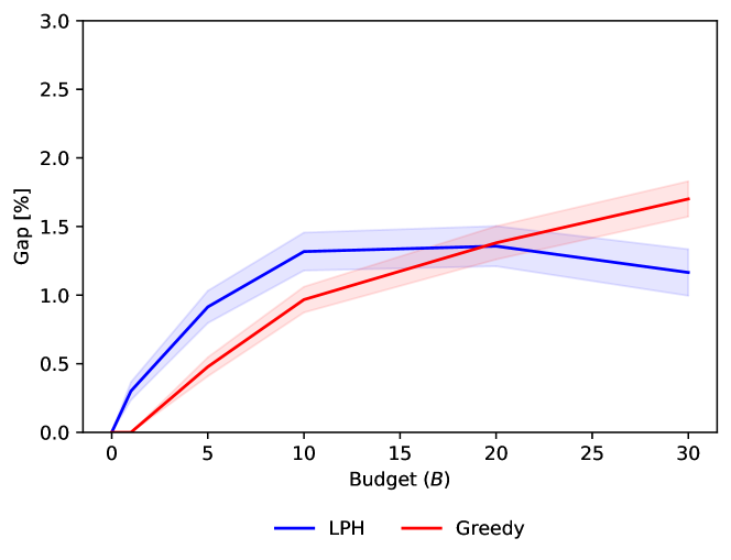
(b) $|{\mathcal{C}}|=10$

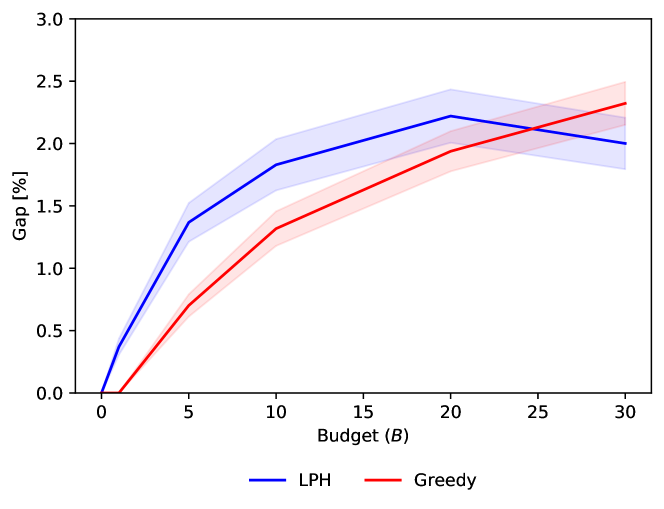
(c) $|{\mathcal{C}}|=15$

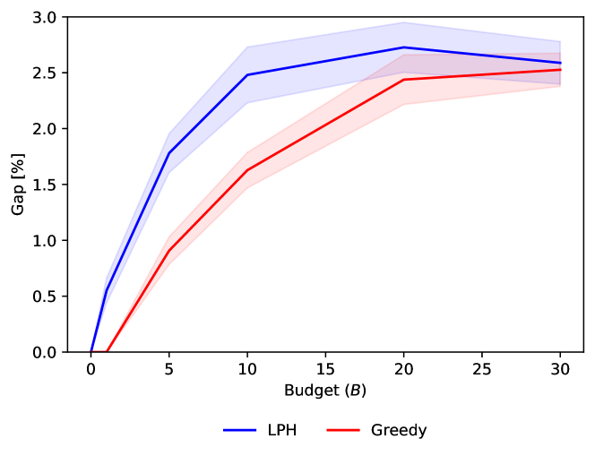
(d) $|{\mathcal{C}}|=20$

Figure 1: Optimality Gap for the Heuristics

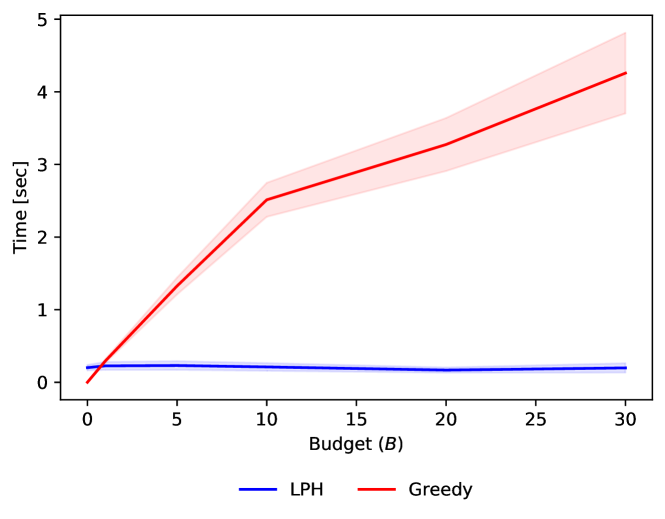
(a) $|{\mathcal{C}}|=5$

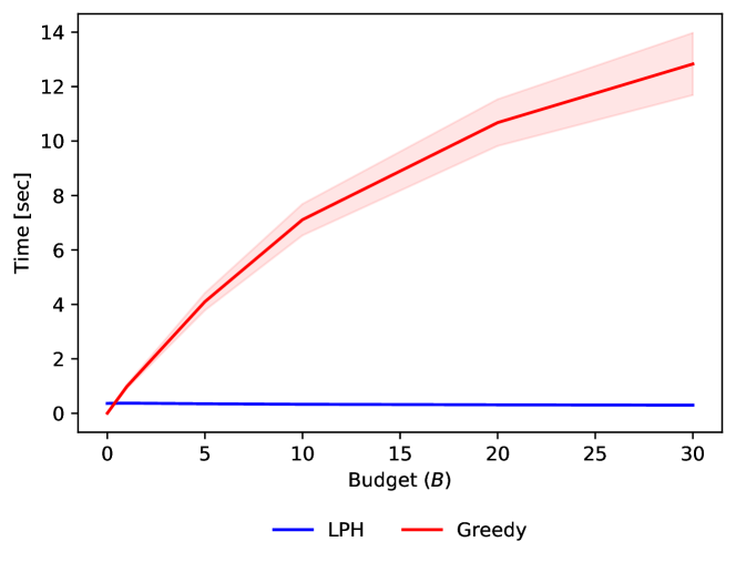
(b) $|{\mathcal{C}}|=10$

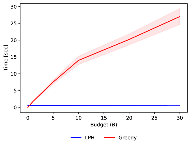
(c) $|{\mathcal{C}}|=15$

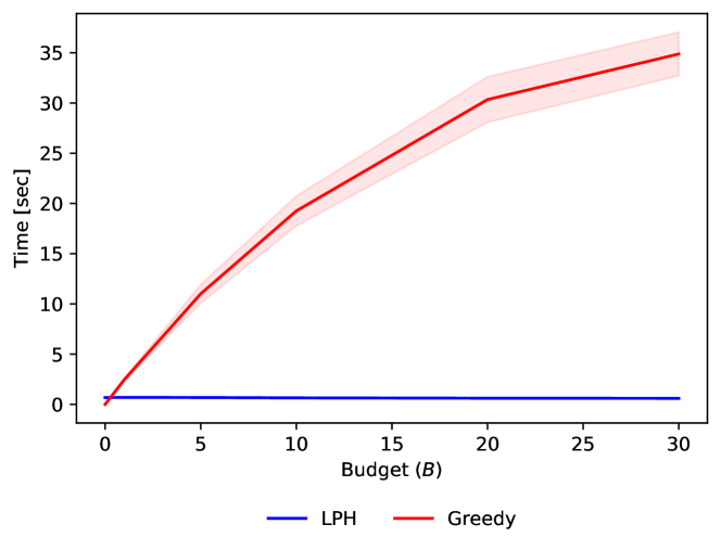
(d) $|{\mathcal{C}}|=20$

Figure 2: Running Time for the Heuristics

Overall, our simulation results suggest that Cpm is the best approach to solve larger instances of the problem and that LPH is the best heuristic for even larger instances. This heuristic is very relevant in terms of practical use as it is simple to describe, extremely efficient, and capable of achieving good quality solutions.

5 Application to School Choice in Chile

To illustrate the potential benefits of capacity expansion, we adapt our framework to the Chilean school choice system. This system, introduced in 2016 in the southernmost region of the country (Magallanes), was fully implemented in 2020 and serves close to half a million students and more than eight thousand schools each year.

The Chilean school choice system is a good application for our methodology for multiple reasons. First, the system uses a variant of the student-proposing Deferred Acceptance algorithm, which incorporates priorities and overlapping quotas. Our framework can include all the features of the Chilean system, including the block application, the dynamic siblings’ priority, etc. We refer to Correa et al. (2022) for a detailed description of the Chilean school choice system and the algorithm used to perform the allocation. Second, the Ministry of Education manages all schools that participate in the system and thus can ask them to modify their vacancies within a reasonable range. Finally, the system is currently being redesigned, and we are collaborating with the authorities to include some of the ideas introduced in our work.

5.1 Data and Simulation Setting

We consider data from the admission process in 2018. Specifically, we focus on the southernmost region of the country as it is the region where all policy changes are first evaluated. Moreover, we restrict the analysis to Pre-K for two reasons: (i) it is the level with the highest number of applicants, as it is the first entry level in the system, and (ii) to speed up the computation. In Table 2, we report summary statistics about the instance, and we compare it with the values nationwide for the same year.

Table 2: Instance for Evaluation

Region	Students	Schools	Applications
Magallanes Pre-K	1389	43	4483
Overall Pre-K	84626	3465	256120
Overall (all levels)	274990	6421	874565

We perform our simulations varying the budget $B\in\left\{0,1,\ldots,30\right\}$ and the penalty for unassigned students $r_{s,\emptyset}$. For the latter, we consider two cases: (i) $r_{s,\emptyset}=\left|{\mathcal{C}}\right|+1$ for all $s\in{\mathcal{S}}$, and (ii) $r_{s,\emptyset}=\left|\succ_{s}\right|+1$ for all $s\in{\mathcal{S}}$. Notice that the two values for $r_{s,\emptyset}$ cover two extreme cases. When $r_{s,\emptyset}=\left|{\mathcal{C}}\right|+1$ (or any large number), the model will use the extra vacancies to ensure that a student that was previously unassigned gets assigned. In contrast, when $r_{s,\emptyset}=\left|\succ_{s}\right|+1$, the model will (most likely) assign the extra seat to the school that leads to the largest chain of improvements. Hence, from a practical standpoint, which penalty to use is a policy-relevant decision that must balance access and improvement.

5.2 Results

We report our main simulation results in Figure 3. For each budget, we plot the number of students who (1) enter the system, i.e., who are not initially assigned (with $B=0$), but are assigned to one of their preferences when capacities are expanded; (2) improve, i.e., students who are initially assigned to some preference but improve their preference of assignment when capacities are expanded; and (3) overall, which is the total number of students who benefit relative to the baseline and is equal to the sum of the number of students who enter and improve.

First, we confirm that all initially assigned students (with $B=0$) get a school at least as preferred when we expand capacities. Second, increasing capacities with a high penalty primarily benefits initially unassigned students. In contrast, students who improve their assignments are the ones who most benefit when the penalty is low. Third, we observe that the total number of students who benefit (in green) is considerably larger than the number of additional seats (dashed). The reason is that an extra seat can lead to a chain of improvements that ends either on a student that enters the system or in a school that is under-demanded. Finally, we observe that the total number of students who gain from the additional seats is not strictly increasing in the budget. Indeed, the number may decrease if the extra seat allows a student to dramatically enhance their assignment (e.g., moving from being unassigned to assigned to their top preference). This effect on the objective could be larger than that of a chain of minor improvements involving several students, and thus the number of students who benefit may decrease.

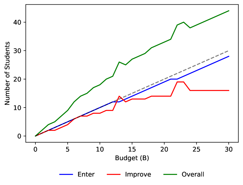
(a) $r_{s,\emptyset}=\left|{\mathcal{C}}\right|+1$

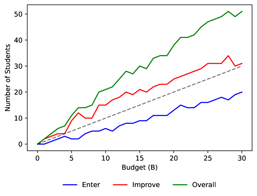
(b) $r_{s,\emptyset}=\left|\succ_{s}\right|+1$

Figure 3: Effect for Students

In Figure 4, we analyze the impact of expanding capacities on the number of schools with increased capacity and the maximum number of additional seats per school. We observe that the number of schools with extra seats remains relatively stable as we increase the budget. In addition, we observe that the maximum number of additional seats in a given school increases with the budget. This is because students’ preferences are highly correlated (i.e., students have similar preferences) and, thus, a few over-demanded schools concentrate the extra seats added to the system. Finally, the latter effect is more prominent when the penalty is lower.

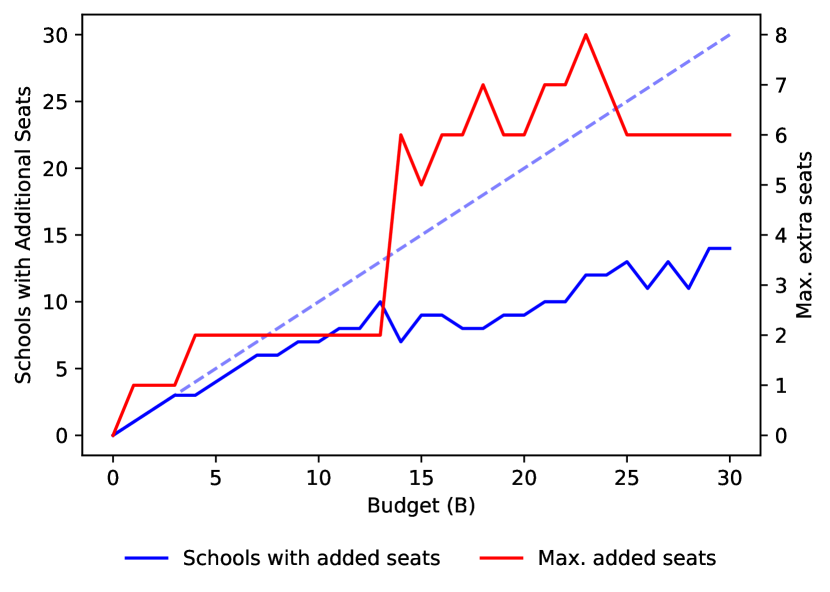
(a) $r_{s,\emptyset}=\left|{\mathcal{C}}\right|+1$

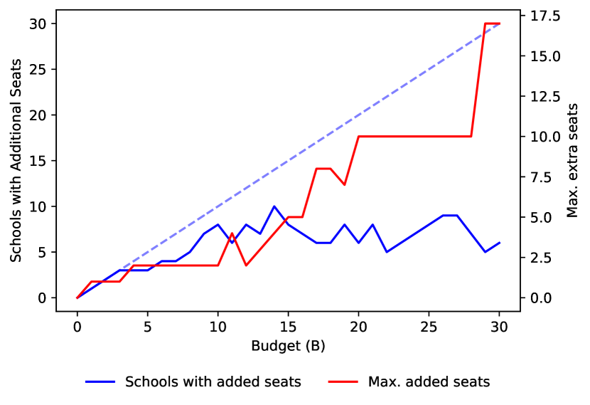
(b) $r_{s,\emptyset}=\left|\succ_{s}\right|+1$

Figure 4: Effect for Schools

5.2.1 Practical Implementation.

A valid concern from policymakers is that our approach would assign most extra seats to a few over-demanded schools if preferences are highly correlated and the penalty of having unassigned students is small. As a result, our solution would not be feasible in practice. To rule out this concern, we adapt our model and include the new set of constraints

$$t_{c}\leq b_{c},\quad\forall\ c\in{\mathcal{C}},$$

where $b_{c}$ is the maximum number of additional seats that can be allocated to school $c$.

In Figure 5, we compare the gap between the optimal (unconstrained) solution and the values obtained when considering $b_{c}\in\left\{2,5,10\right\}$ for all $c\in{\mathcal{C}}$ and $r_{s,\emptyset}=\left|\succ_{s}\right|+1$ for all $s\in{\mathcal{S}}$. First, we observe that the gap increases for $b_{c}\in\left\{2,5\right\}$ as we increase the budget, while it does not change for $b_{c}=10$. This result suggests that the problem has many optimal solutions and, thus, we can select one that does not over-expand some schools. Second, we observe that the overall gap is relatively low (max of 0.8%), which suggests that we can include the practical limitations for schools without major losses of performance. In Appendix 13, we discuss some model extensions to incorporate other relevant aspects from a practical standpoint.

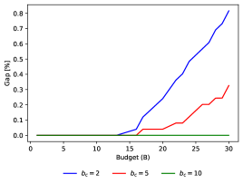
Figure 5: Effect of Bounds on Expansion

5.2.2 Heuristics.

For each value of the budget, in Figure 6, we report the gap obtained relative to the optimal policy. Consistent with the results in Section 4, Greedy performs better than LPH for low values of the budget, but this reverses as the budget increases. Hence, we conclude that LPH can be an effective approach for large instances and large values of $B$. This could be particularly relevant when applying our framework to other more populated regions, such as the Metropolitan region, where close to 250,000 students apply each year.

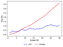
Figure 6: Heuristics: Optimality Gap

5.3 Further Insights: An Application to the Chilean College Admission System

Since early 2023, we have collaborated with the Ministry of Education of Chile (MINEDUC) and the “Sistema Único de Admisión” (SUA; the Chilean college board) in several applications of our framework. Specifically, we have been working on two main projects: (i) evaluating which schools should be overcrowded in order to downsize under-demanded schools, and (ii) evaluating minimum requirements regarding seats to offer to under-represented groups. The former problem can be addressed by adapting what we discussed in the previous section, so we focus on the latter.

The centralized part of the Chilean college admissions system includes an affirmative action policy (called “Programa PACE”), which consists of reserved seats for under-represented students (over 10,000 students each year) and special funds for the institutions where these students enroll. To be eligible to participate in this affirmative action policy (and potentially receive these funds), universities must commit to reserving a specified number of seats following specific guidelines defined by MINEDUC, e.g., a minimum number of reserved seats per program and a minimum total number of reserved seats across all their programs. Conditional on satisfying these requirements, universities can independently decide how many seats to reserve. Many universities meet these requirements by fulfilling the minimum requirement (of one reserved seat) per program and then devoting the additional required seats to under-demanded programs. As a result, only 18% of the reserved seats were used in the admissions process of 2022-2023.

To tackle this issue, we have been collaborating with MINEDUC to evaluate the effects of potential changes to these requirements. Since we do not know what the objective function of each university is (and, thus, how they allocate these reserved seats), MINEDUC asked us to evaluate different combinations of requirements (e.g., a minimum number of seats for the most popular programs, changes to the way to define the total number of reserved seats to offer, etc.) and objective functions (e.g., minimize the preferences of assignment, maximize the utilization of the reserved seats, maximize the cutoffs, maximize the average scores in Math and Verbal of the admitted students, among others) to obtain a wide range of possible outcomes that could result from each set of requirements.

For each of these combinations (of requirements, objectives, and other specific parameters), we adapted the framework described in this work and performed simulations considering the data from the admissions process of 2022-2023. Using current data to evaluate the implementation of these requirements in future years is without major loss, since students’ preferences are relatively stable over time and, thus, the reported preferences of one year are the best predictor of those in the coming years. Finally, note that having a methodology to solve the problem relatively fast was instrumental in performing this analysis, as it required hundreds of simulations in a fairly large instance.

This application showcases the flexibility of our methodology to answer different questions and stresses the need to solve these problems in a reasonable time.

6 Conclusions

We study how centralized clearinghouses can jointly decide the allocation of additional seats and find a stable matching. To accomplish this, we introduce the stable matching problem under capacity planning and devise integer programming formulations for it. We show that all natural formulations involve quadratic constraints and provide linearizations for them. Then, we develop a non-compact mixed-integer linear program (BB-cap) and prove that it correctly models our problem. Building on this key result, we introduce a cutting-plane algorithm to solve BB-cap. At the core of our cutting-plane algorithm is a new separation method, which finds the most violated comb constraint for each school in polynomial time and, when the objective is the student-optimal stable matching, prunes the set of schools for which violated comb constraints may exist. Finally, we show and discuss several properties of our mechanism, including how the cardinality of the allocation varies with the penalty (and how this can be used to prioritize different goals), some incentive properties and also the mechanism’s monotonicity.

Through an extensive numerical study, we find that our cutting-plane algorithm significantly outperforms all the state-of-the-art formulations in the literature. In addition, we find that one of the two heuristics that we propose (LPH) consistently finds near-optimal solutions in few seconds. These results suggest that our cutting-plane method and the LPH heuristic can be practical approaches depending on the size of the problem. Moreover, we adapted our framework to solve an instance of the Chilean school choice problem. Our results show that each additional seat can benefit multiple students. However, depending on how we penalize having unassigned students in the objective, the set of students who benefit from the extra seats changes. Indeed, we have theoretically shown that if we consider a large penalty, the optimal solution prioritizes access, i.e., assigning students that were previously unassigned. In contrast, if that penalty is low, we proved that the optimal solution prioritizes improvement, i.e., benefiting students’ preference of assignment as much as possible. Hence, which penalty to consider is a policy-relevant decision that depends on the objective of the clearinghouse.

Overall, our results showcase how to extend the classic stable matching problem to incorporate capacity decisions and how to solve the problem effectively. Our methodology is flexible to accommodate different settings, such as capacity reductions, allocations of tuition waivers, quotas, secured enrollment, and arbitrary constraints on the extra seats per school (see Appendix 13 for more details). Moreover, we can adapt our framework to other stable matching settings, such as the allocation of budgets to accommodate refugees, the assignment of scholarships or tuition waivers in college admissions, and the rationing of scarce medical resources. All of these are exciting new areas of research in which our results can be used.

This work was funded by FRQ-IVADO Research Chair in Data Science for Combinatorial Game Theory, and the NSERC grant 2019-04557.

Appendix

7 Missing Proofs and Other Results

7.1 Proof of Lemma 3.1.

We begin by observing that Baïou and Balinski (2000) show that the feasible region of max-hrt corresponds to the set of stable matchings. Therefore, in the following proof, we only need to focus on proving the equivalence between the student-optimal matching and a matching minimizing the sum of the students’ rank over the set of stable matchings.

If: In a student-optimal stable matching, each student is assigned to the best school they could achieve in any stable matching Gale and Shapley (1962). Thus, each unassigned student is unassigned in every stable matching. Moreover, by the Rural Hospital Theorem Roth (1982, 1984), Gale and Sotomayor (1985), Roth (1986), the same students are assigned in all stable matchings. Suppose that $\mu$ is the student-optimal stable matching but its corresponding binary encoding is not optimal to max-hrt. Let $x^{\prime}$ be an optimal solution max-hrt and let $\mu^{\prime}=\{(s,c)\in{\mathcal{E}}:x^{\prime}_{s,c}=1\}$ be the associated matching. Hence, the following inequality holds: $\sum_{(s,c)\in\mu}r_{s,c}>\sum_{(s,c)\in\mu^{\prime}}r_{s,c}$. This means that there is at least one student $s^{\prime}$ who prefers the stable matching $\mu^{\prime}$ to the stable matching $\mu$, which is a contradiction.

Only if: Let $\mu$ be a (stable) matching corresponding to an optimal solution of max-hrt. As before, by the Rural Hospital Theorem, we observe that the set of students unassigned in $\mu$ is the same set of students unassigned in every stable matching. Hence, the set of assigned students in $\mu$, is the same set for every stable matching. Let us suppose, again by contradiction, that $\mu$ is not a student-optimal stable matching. Let $\mu^{\prime}$ be a student-optimal stable matching. Denote by $S^{\prime}$ the set of students whose assignment to schools differs in the two matchings. By construction, the objective value of max-hrt for ${\mathcal{S}}\setminus S^{\prime}$ is the same in both $\mu$ and $\mu^{\prime}$:

$$\sum_{(s,c)\in\mu:\ s\in{\mathcal{S}}\setminus S^{\prime}}r_{s,c}=\sum_{(s,c)\in\mu^{\prime}:\ s\in{\mathcal{S}}\setminus S^{\prime}}r_{s,c}.$$

Furthermore, $S^{\prime}$ is the disjoint union of the following two sets of students: $S_{1}^{\prime}$, the set of assigned students who prefer their school in $\mu^{\prime}$, and $S_{2}^{\prime}$, the set of assigned students who prefer their school in $\mu$. By Gale and Shapley (1962), $\mu^{\prime}$ is a stable matching in which all students are assigned the best school they could achieve in any stable matching. Therefore, the set $S_{2}^{\prime}$ is empty. Hence, $S^{\prime}=S_{1}^{\prime}$, and by hypothesis

$$\sum_{(s,c)\in\mu:\ s\in S_{1}^{\prime}}r_{s,c}<\sum_{(s,c)\in\mu^{\prime}:\ s\in S_{1}^{\prime}}r_{s,c}.$$

However, from the definition of $S_{1}^{\prime}$, $r_{s,\mu^{\prime}(s)}\leq r_{s,\mu(s)}$ for every $s\in S_{1}^{\prime}$, which leads to a contradiction.

7.2 Proof of Theorem 3.4

The constraints that do not involve the linearization terms $\alpha_{s,c}$ or $\beta_{s,c,c^{\prime}}$ are trivially satisfied by a feasible solution in both formulations. Therefore, we will restrict our analysis to the remaining constraints. Let $(\mathbf{x},\mathbf{t},$$\alpha$) be a feasible solution of the relaxed aggregated linearized program. It is easy to verify that by defining $\bar{\beta}_{s,c,c^{\prime}}=\alpha_{s,c}\cdot x_{s,c^{\prime}}$ for every $s\in{\mathcal{S}},\,c\in{\mathcal{C}}$ and $c^{\prime}\succeq_{s}c$, the constraints of the relaxed non-aggregated linearization are all met.

7.3 Missing Proofs in Section 3.3

7.3.1 Proof of Theorem 3.5

Before proving Theorem 3.5, we show a couple of lemmata. In the following lemma, we show that if a capacity variable is set to 1, then all the comb constraints determined by supersets are satisfied.

Lemma 7.1

Let $\bar{\mathbf{x}}\in\{0,1\}^{{\mathcal{E}}}$ be a stable matching for some vector of extra seats $\bar{\mathbf{y}}\in\{0,1\}^{{\mathcal{C}}\times\{0,\ldots,B\}}$. If $\bar{y}_{c}^{k}=1$ then all constraints (6b) for the combs in $C_{c}(k+\alpha)$ with $\alpha>0$ are satisfied.

Proof 7.2

Proof. When $\bar{y}_{c}^{k}=1$, the right-hand-side of constraints (6b) for combs in $C_{c}(k+\alpha)$ is $q_{c}$. Thus, we need to show that the left-hand-side of these constraints is guaranteed to be greater than or equal to $q_{c}$. By the definition of comb, for all $C\in C_{c}(k+\alpha)$ there is $\hat{C}\in C_{c}(k)$ such that $\hat{C}\subseteq C$. Hence,

$$\sum_{(s,c^{\prime})\in C}\bar{x}_{s,c^{\prime}}\geq\sum_{(s,c^{\prime})\in\hat{C}}\bar{x}_{s,c^{\prime}}\geq q_{c}+k\geq q_{c},$$

where the second inequality follows from the hypothesis that $\bar{\mathbf{x}}$ is stable for $\bar{\mathbf{y}}$.

We now prove the analogous of the previous lemma, but for comb constraints defined by subsets.

Lemma 7.3

Let $\bar{\mathbf{x}}\in\{0,1\}^{{\mathcal{E}}}$ be a stable matching for some vector of extra seats $\bar{\mathbf{y}}\in\{0,1\}^{{\mathcal{C}}\times\{0,\ldots,B\}}$. If $\bar{y}_{c}^{k}=1$, then all constraints (6b) for combs in $C_{c}(k-\alpha)$ with $\alpha<k$ are satisfied.

Proof 7.4

Proof. When $\bar{y}_{c}^{k}=1$, the right-hand-side of constraint (6b) for each comb $C\in C_{c}(k-\alpha)$ is $q_{c}$. Thus, we need to show that the left-hand-side of this constraint is guaranteed to be greater than or equal to $q_{c}$. Let $(s,c)$ be the base of the comb $C$.

First, we show the result when there is $\hat{C}\in C_{c}(k)$ such that $C\subseteq\hat{C}$. By the definition of generalized comb (see Subsection 3.3), $C$ contains the shaft $S^{k-\alpha}(s,c)$. Consequently, since $\hat{C}$ contains $C$, if $(s^{\prime},c)$ is the base of $\hat{C}$, then $S^{k-\alpha}(s,c)\subseteq S^{k}(s^{\prime},c)$.

Let $T_{s_{r}}$ for $r=1,\ldots,q_{c}+k$ be the set of teeth for comb $\hat{C}$ which (obviously) contains the teeth of comb $C$. Therefore,

$$\hat{C}=\bigcup_{r=1}^{q_{c}+k}T_{s_{r}}\cup S^{k}(s^{\prime},c).$$

Let $T\subseteq\{1,\ldots,q_{c}+k\}$ be the set of indices corresponding to the teeth of $C$; thence, $|T|=q_{c}+k-\alpha$. There are two cases:

• If there is $r\in T$ such that

  $$\sum_{(s_{r},j)\in T_{s_{r}}}\bar{x}_{{s_{r}},j}=0,$$

  then student $s_{r}$ is matched with a school that they prefer less than school $c$. Under the stable matching $\bar{\mathbf{x}}$, this is only possible if school $c$ is matched with exactly $q_{c}+k$ students that school $c$ prefers more than student $s_{r}$:

  $$\sum_{(i,c)\in S^{k-\alpha}(s,c)}\bar{x}_{i,c}=q_{c}+k.$$

  Since $S^{k-\alpha}(s,c)\subseteq C$, then

  $$\sum_{(i,j)\in C}\bar{x}_{i,j}\geq q_{c}+k\geq q_{c}.$$

• If $\sum_{(s_{r},j)\in T_{s_{r}}}\bar{x}_{{s_{r}},j}=1$ for all $r\in T$, then

  $$\sum_{r\in T}\sum_{(s_{r},j)\in T_{s_{r}}}\bar{x}_{s_{r},j}=|T|=q_{c}+k-\alpha\geq q_{c}.$$

  Since $\bigcup_{r\in T}T_{s_{r}}\subseteq C$ the results holds.

Second, we prove the lemma when no comb of $C_{c}(k)$ contains $C$. Then, such situation can only occur if it is not possible to find a shaft $S^{k}(s^{\prime},c)$ where $s^{\prime}=s$ or $s\succ_{c}s^{\prime}$. This means that the number of seats $q_{c}+k$ is greater than the number of students that the school ranks. Consequently, the set $C_{c}(k)$ is empty and there is nothing to prove.

We now prove our main result in this section.

Proof 7.5

Proof of Theorem 3.5. The preceding lemmas lead us to conclude the statement when the integrality of $\mathbf{x}$ is imposed: for each fixed $\mathbf{y}$, only the comb constraints (6b) associated to the overall capacity of each school are enforced; the remaining are redundant. When the integrality of $\mathbf{x}$ is relaxed, the statement follows directly from Baïou and Balinski (2000): when $\mathbf{y}$ is fixed, the comb inequalities for the associated capacities provide the convex hull of stable matchings for $\Gamma_{\mathbf{t}}$ where $t_{c}=\sum_{k=0}^{B}y_{c}^{k}$ for all $c\in{\mathcal{C}}$. Thus, as long as the number of seats for each school is integer, constraints (6b) contain the comb constraints from Baïou and Balinski (2000) for $\Gamma_{\mathbf{t}}$.

7.3.2 Missing Proofs in Section 3.3.1

Proof 7.6

Proof of Lemma 3.6. We prove that $c$ is fully-subscribed in $\mathbf{x}^{\star}$ by contradiction. Let $(s,c)$ be a fractional blocking pair for $\mathbf{x}^{\star}$, where $c$ is an under-subscribed school in $\mathbf{x}^{\star}$. Let $s$ be such that $x_{s,c^{\prime}}^{\star}>0$ and $c\succ_{s}c^{\prime}$. So $s$ prefers $c$ over $c^{\prime}$. Moreover, $c$ has some available capacity which would allow to increase $x_{s,c}^{\star}$ by decreasing $x_{s,c^{\prime}}^{\star}$. Clearly, such modification would decrease the objective value of the main program. This contradicts the optimality of $\mathbf{x}^{\star}$.

Proof 7.7

Proof of Lemma 3.7. Let ${\mathcal{C}}^{\prime}$ be the set of fully-subscribed schools in $\mu^{\star}$ and ${\mathcal{S}}^{\prime}$ be the set of students matched to the schools ${\mathcal{C}}^{\prime}$ in $\mu^{\star}$. We denote by ${\mathcal{C}}^{\prime\prime}$ and ${\mathcal{S}}^{\prime\prime}$ the complementary sets of ${\mathcal{C}}^{\prime}$ and ${\mathcal{S}}^{\prime}$ respectively. Let us analyze the matches in ${\mathcal{S}}^{\prime}$. First, note that for every student $s\in{\mathcal{S}}^{\prime}$ we have $\sum_{c\succeq\mu^{\star}(s)}x^{\star}_{s,c}=1$, i.e., student $s$ must be matched in $\mathbf{x}^{\star}$ to some school that she prefers at least as much as $\mu^{\star}(s)\in C^{\prime}$. This is because $\mathcal{J}$ contains all the comb constraints of the schools in ${\mathcal{C}}^{\prime}$. Second, every student $s\in{\mathcal{S}}^{\prime}$ must be matched in $\textbf{x}^{\star}$ to a school that is in ${\mathcal{C}}^{\prime}$, i.e., $\sum_{c\in{\mathcal{C}}^{\prime}}x^{\star}_{s,c}=1$. This is because, otherwise, $s$ would create a blocking pair in $\mu^{\star}$ with a under-subscribed school in ${\mathcal{C}}^{\prime\prime}$ due to our first argument. As a consequence of the second point, we cannot have $x^{\star}_{s,c}>0$ for a student $s\in{\mathcal{S}}^{\prime\prime}$ and a school $c\in{\mathcal{C}}^{\prime}$. This is because we proved above that all students in ${\mathcal{S}}^{\prime}$ are matched in ${\mathcal{C}}^{\prime}$ and schools in ${\mathcal{C}}^{\prime}$ are fully-subscribed. All the above imply that we can consider ${\mathcal{S}}^{\prime}$ and ${\mathcal{C}}^{\prime}$ as a sub-instance of the problem and the integrality of $\mathbf{x}^{\star}$ is given by the comb constraints. Because of optimality, $\mu^{\star}$ and $\mathbf{x}^{\star}$ must coincide in ${\mathcal{S}}^{\prime}$ and ${\mathcal{C}}^{\prime}$. Let us now analyze the assignments of the students in ${\mathcal{S}}^{\prime\prime}$. First, note that the integrality of $\mathbf{x}^{\star}$ in the sub-instance defined by ${\mathcal{S}}^{\prime\prime}$ and ${\mathcal{C}}^{\prime\prime}$ is given by the integrality of the matching polytope without stability constraints. Now, we will show that the assignments coincide in both $\mu^{\star}$ and $\textbf{x}^{\star}$. By contradiction, assume that the students in ${\mathcal{S}}^{\prime\prime}$ are matched differently in $\textbf{x}^{\star}$ and in $\mu^{\star}$. First, if there is a student $s\in{\mathcal{S}}^{\prime\prime}$ that prefers a school $c$ over $\mu^{\star}(s)$, then $(s,c)$ would be a blocking pair in $\mu^{\star}$ because $c$ is under-subscribed in $\mu^{\star}$, which is not possible. Therefore, every student $s\in{\mathcal{S}}^{\prime\prime}$ weakly prefers $\mu^{\star}(s)$ over their assignment in $\textbf{x}^{\star}$, and, by the hypothesis in our contradiction argument, there is at least one student $s$ that strictly prefers $\mu^{\star}(s)$ over their match in $\textbf{x}^{\star}$ (i.e., the two schools are different). Given that ${\mathcal{S}}^{\prime\prime}$ and ${\mathcal{C}}^{\prime\prime}$ form a separate sub-instance, we can rearrange the matching $\textbf{x}^{\star}$ of every student in ${\mathcal{S}}^{\prime\prime}$ by matching the student to her matching in $\mu^{\star}$. This new matching would have a lower objective than the one of $\textbf{x}^{\star}$, which would violate its optimality. Therefore, both $\mu^{\star}$ and $\mathbf{x}^{\star}$ also coincide in ${\mathcal{S}}^{\prime\prime}$ and ${\mathcal{C}}^{\prime\prime}$.

Proof 7.8

Proof of Lemma 3.8. Suppose that the statement is false. Then, for every school $c$ in block($\mathbf{x}^{\star}$), and for every student $s$ more preferred by $c$ to the least preferred student in $\text{exceeding}(c)$, $s$ has the tooth evaluated to 1. By Lemma 3.6, we know that the fractional blocking pairs must all involve a school that is fully-subscribed in $\mathbf{x}^{\star}$. Among these schools, it is sufficient to focus our attention on the schools $c\in C$ such that there exists $s\in S$ with $x^{\star}_{s,c}>0$ and student $s$ is not matched to $c$ in $\mu^{\star}$. Therefore, for these schools the set of exceeding students is non-empty.

We now observe that, by hypothesis, every school $c$ in block($\mathbf{x}^{\star}$), has the property that all the teeth are evaluated to 1 until the least preferred exceeding student. This implies that all the combs in $C_{c}(\mathbf{t}_{c}^{\star})$ are not violated since such combs are composed by $q_{c}+t_{c}^{\star}$ teeth. Hence, $\mathbf{x}^{\star}$ is a stable matching with a better objective for the students than the student-optimal stable matching.

Proof 7.9

Proof of Theorem 3.9.

We start this proof by showing that for each school $c\in$ block($\mathbf{x}^{\star}$), Steps 5-21 of Algorithm 2 provide the comb solving Formulation (8) in $\mathcal{O}(n\cdot\bar{q})$.

First, let us observe that the search for the least valued comb in $C_{c}(t_{c}^{\star})$ terminates in a finite number of steps because the preference list $\succ_{c}$ is finite. At the beginning of every cycle in Step 8, we select a student $s^{\prime}$. By the end of the $(q_{c}+t_{c}^{\star})$-th iteration, the comb $C$ is the smallest valued comb in $C_{c}(t_{c}^{\star})$ with a base preferred at least as $s^{\prime}$ (i.e., the student at the base of the comb is ranked equal or less than $s^{\prime}$). If we prove this statement, we prove that the algorithm solves Formulation (8) for $c$.

Base: At the $(q_{c}+t_{c}^{\star})$-th iteration, we create comb $C$ at Step 13. The base of comb $C$ is the student $s^{\prime}$ that is ranked $q_{c}+t_{c}^{\star}$ by $c$, and the bases of the other $q_{c}+t_{c}^{\star}-1$ teeth are the students preferred more than $s^{\prime}$. Since this comb is the only possible that we can create with a base preferred more or equal than $s^{\prime}$, it is also the least valued comb possible.

Inductive step: The inductive hypothesis states that at the end of iteration $l\geq q_{c}+t_{c}^{\star}$, after selecting student $s^{\prime}$, the selected comb $C$ is the comb with the lowest value among all combs with a base student preferred equal to or more than $s^{\prime}$. We want to prove that at the end of step $l+1$, the algorithm selects the comb with lowest value among all combs with a base student ranked less or equal than $(l+1)$. Let $s^{\prime}$ be the student ranked $l+1$ and let $s^{\star}$ be the student in $\mathcal{T}$ with the highest valued $T^{-}$. We need to verify if adding $T^{-}(s^{\prime},c)$ to $\mathcal{T}$ may produce a comb of smaller value than the one recorded. If $T^{-}(s^{\prime},c)\geq T^{-}(s^{\star},c)$, then adding $s^{\prime}$ in $\mathcal{T}$ would produce a comb with equal or higher value. Otherwise, $T^{-}(s^{\prime},c)<T^{-}(s^{\star},c)$, and adding ${}^{\prime}s$ in $\mathcal{T}$ may provide a better comb. If $T^{-}(s^{\prime},c)<T^{-}(s^{\star},c)$, then we create a new comb $C^{\prime}$ with base in $(s^{\prime},c)$ and teeth in $\mathcal{T}\setminus\{s^{\star}\}$. Any other choice of teeth is sub-optimal for the base $(s^{\prime},c)$ since they are the least valued $q_{c}+t_{c}^{\star}$ teeth among those in the first $l+1$ positions. If the new comb $C^{\prime}$ has value smaller than the comb $C$, then we have found the best comb among those with base ranked at most $l+1$.

If $s^{\prime}$ is the least preferred exceeding student, then all the combs with base $s^{\prime}$ are valued at least $q_{c}+t_{c}^{\star}$ since $c$ is a fully subscribed school. Hence, any comb that may be selected with such a base would not be violated, and we can terminate our search.

To establish the correctness of Algorithm 2, it remains to show that it determines the violated combs (if any) that eliminate the input solution. First, the algorithm terminates in a finite number of steps because $|\text{block}(\mathbf{x}^{\star})|\leq|{\mathcal{C}}|=m$ and $|\succ_{c}|\leq|{\mathcal{S}}|=n$. Second, by Lemma 3.8 we only need to focus our attention on the fully-subscribed schools in block($\mathbf{x}^{\star}$). Thus, Algorithm 2 returns the most violated comb constraint for those schools.

Running-time analysis.

The procedure for finding $\underline{s}$ takes at most $n$ operations. The inner for loop (Step 8) takes at most $n$ rounds and the most expensive computation within it is placing $s^{\prime}$ in $\mathcal{T}$ to maintain the list $\mathcal{T}$ is descending order according to the values $v_{s,c}$. Note that this task can be performed by comparing $s^{\prime}$ with at most each element in $\mathcal{T}$, i.e., in a number of operations equal to $|\mathcal{T}|=q_{c}+t_{c}^{\star}$. Hence, the number of elementary operations for finding the most violated comb of school $c$ is at most $\mathcal{O}(n\cdot(q_{c}+t_{c}^{\star}))$. To conclude, we observe that, in Algorithm 2, the computation of block($\mathbf{x}^{\star}$) at Step 4 can take at most $\mathcal{O}(m\cdot n)$ time, i.e., the running time of the Deferred Acceptance algorithm. Moreover, as proved above, finding the least valued comb of a school in block($\mathbf{x}^{\star}$) can take at most $\mathcal{O}(n\cdot(q_{c}+t_{c}^{\star}))$ time. Hence, Algorithm 2 can take at most $\mathcal{O}(m\cdot n\cdot\bar{q})$ time, where $\bar{q}=\max\limits_{c\in\text{block}(\mathbf{x}^{\star})}\{q_{c}+t^{\star}_{c}\}$.

7.4 Properties of the Mechanism

7.4.1 Cardinality

A crucial aspect of the solutions of Formulation 2 is that they largely depend on the value of $r_{s,\emptyset}$, i.e., the penalty for having unassigned students. We emphasize that $r_{s,\emptyset}$ does not indicate the position of $\emptyset$ in the ranking of $s$ over schools, but a penalty value for being unassigned. One could expect that for larger penalty values, the optimal solution will prioritize access by matching initially unassigned students and increasing the cardinality of the match. In contrast, for smaller penalty values, the focus will be on the improvement of previously assigned students by prioritizing chains of improvement that result in multiple students obtaining a better assignment than the initial matching with no extra capacities. In Theorems 7.10 and 7.12 we formalize this intuition.

Theorem 7.10

There is a sufficiently small and finite $r_{s,\emptyset}$ for all $s\in{\mathcal{S}}$ such that the optimal solution of Formulation (2) returns a minimum cardinality student-optimal stable matching.

Proof 7.11

Proof. Let $\mu^{0}$ be the student-optimal assignment when there is no budget, and let $M(\mu)=\left\{s\in{\mathcal{S}}:\mu(s)\in{\mathcal{C}}\right\}$ be the set of students assigned in match $\mu$. In addition, let $r_{s,\emptyset}=r_{\emptyset}=\left|{\mathcal{S}}\right|\cdot(1-\xi)$, where $\xi=\max_{s\in{\mathcal{S}}}\left\{\left|\succ_{s}\right|\right\}$ is the maximum length of a list of preferences among all students.

Let $\mu^{*}$ be the optimal allocation implied by the optimal solution of the problem $(\mathbf{x}^{*},\mathbf{t}^{*})$ considering a budget $B$ and the aforementioned penalties. To find a contradiction, suppose that there exists an alternative match $\mu^{\prime}$ that uses the entire budget $B$ and that satisfies $\left|M(\mu^{*})\right|>\left|M(\mu^{\prime})\right|$. Without loss of generality, suppose that $\left|M(\mu^{*})\right|=\left|M(\mu^{\prime})\right|+1$. We know that $M(\mu^{0})\subseteq M(\mu^{*})$ and $M(\mu^{0})\subseteq M(\mu^{\prime})$, since no student who was initially assigned can result unassigned when capacities are expanded. Then, the difference in objective function between $\mu^{*}$ and $\mu^{\prime}$ can be written as:

$$\begin{split}\Delta=\sum_{(s,c)\in\mu^{*}}r_{s,c}-\sum_{(s,c)\in\mu^{\prime}}r_{s,c}&=\sum_{s\in\left(M(\mu^{*})\cap M(\mu^{\prime})\right)}r_{s,\mu^{*}(s)}-r_{s,\mu^{\prime}(s)}\\ &+\sum_{s\in M(\mu^{*})\setminus M(\mu^{\prime})}r_{s,\mu^{*}(s)}-r_{s,\emptyset}+\sum_{s\in M(\mu^{\prime})\setminus M(\mu^{*})}r_{s,\emptyset}-r_{s,\mu^{\prime}(s)}\\ &+\sum_{s\in S\setminus\left(M(\mu^{*})\cup M(\mu^{\prime})\right)}r_{s,\emptyset}-r_{s,\emptyset}\\ &=\sum_{s\in\left(M(\mu^{*})\cap M(\mu^{\prime})\right)}r_{s,\mu^{*}(s)}-r_{s,\mu^{\prime}(s)}\\ &+\sum_{s\in M(\mu^{*})\setminus M(\mu^{\prime})}r_{s,\mu^{*}(s)}-r_{s,\emptyset}+\sum_{s\in M(\mu^{\prime})\setminus M(\mu^{*})}r_{s,\emptyset}-r_{s,\mu^{\prime}(s)}\\ &\geq\sum_{s\in\left(M(\mu^{*})\cap M(\mu^{\prime})\right)}\left(1-\left|\succ\right|_{s}\right)\\ &+\sum_{s\in M(\mu^{*})\setminus M(\mu^{\prime})}1-r_{s,\emptyset}+\sum_{s\in M(\mu^{\prime})\setminus M(\mu^{*})}r_{s,\emptyset}-\left|\succ_{s}\right|\\ &\geq\left|\left(M(\mu^{*})\cap M(\mu^{\prime})\right)\right|\cdot\left(1-\xi\right)\\ &+\left|M(\mu^{*})\setminus M(\mu^{\prime})\right|\cdot(1-r_{\emptyset})+\left|M(\mu^{\prime})\setminus M(\mu^{*})\right|\cdot(r_{\emptyset}-\xi)\\ &=\left|\left(M(\mu^{*})\cap M(\mu^{\prime})\right)\right|\cdot\left(1-\xi\right)+\left(\left|M(\mu^{\prime})\setminus M(\mu^{*})\right|+1\right)\cdot(1-r_{\emptyset})\\ &+\left|M(\mu^{\prime})\setminus M(\mu^{*})\right|\cdot(r_{\emptyset}-\xi)\\ &\geq\left|\left(M(\mu^{*})\cap M(\mu^{\prime})\right)\right|\cdot\left(1-\xi\right)+\left(\left|M(\mu^{\prime})\setminus M(\mu^{*})\right|\right)\cdot(1-\xi)-r_{\emptyset}\\ &=\left(\left|M(\mu^{*})\cap M(\mu^{\prime})\right|+\left|M(\mu^{\prime})\setminus M(\mu^{*})\right|\right)\cdot\left(1-\xi\right)-r_{\emptyset}\\ &=\left(\left|M(\mu^{*})\cap M(\mu^{\prime})\right|+\left|M(\mu^{\prime})\setminus M(\mu^{*})\right|\right)\cdot\left(1-\xi\right)-\left|{\mathcal{S}}\right|\cdot(1-\xi)\\ &=\left(\left|M(\mu^{*})\cap M(\mu^{\prime})\right|+\left|M(\mu^{\prime})\setminus M(\mu^{*})\right|-\left|{\mathcal{S}}\right|\right)\cdot\left(1-\xi\right)\\ &\geq 0,\\ \end{split}$$ (9)

since both terms are negative as $\left|M(\mu^{*})\cap M(\mu^{\prime})\right|+\left|M(\mu^{\prime})\setminus M(\mu^{*})\right|\leq\left|S\right|$ and $1\leq\xi$. Hence, we obtain that $\Delta\geq 0$, which implies that the objective function evaluated at $\mu^{\prime}$ is strictly less than the objective function evaluated at $\mu^{*}$, which contradicts the optimality of $\mu^{*}$. Finally, note that this derivation holds for any set of penalties such that $r_{s,\emptyset}\leq r_{\emptyset}$, and it also holds for the case when the clearinghouse can decide not to allocate all the budget (as long as this condition applies for both $\mu^{*}$ and $\mu^{\prime}$), so we conclude.

Note that the penalty used in the proof is negative. A negative penalty can be interpreted as the policy-maker willingness to allocate extra capacities to improve the assignment of students already in the system, for example, when merit scholarships are awarded to students who already have a secured position.

By the stability constraints, every student that is initially assigned (i.e., when $B=0$) should be weakly better off when capacities are expanded. Hence, one may think that the minimum cardinality student-optimal stable matching is the one that is optimal for this subset of students. However, as we show in the Example 8.2 in Appendix 8, this is not the case.

On the other hand, in Theorem 7.12, we show that if the penalty values are sufficiently large, then the optimal solution will prioritize access by obtaining a student-optimal stable matching of maximum cardinality.

Theorem 7.12

There is a sufficiently large and finite $r_{s,\emptyset}$ for all $s\in{\mathcal{S}}$ such that the optimal solution of Formulation (2) returns a maximum cardinality student-optimal stable-matching.

Proof 7.13

Proof. Let $\mu^{*}$ be the stable-matching corresponding to the solution $(\mathbf{x}^{*},\mathbf{t}^{*})$. To find a contradiction, suppose there exists another stable matching $\mu^{\prime}$ that has a higher cardinality, i.e., $\left|s\in{\mathcal{S}}\;:\;\mu^{\prime}(s)=\emptyset\right|<\left|s\in{\mathcal{S}}\;:\;\mu^{*}(s)=\emptyset\right|$. By optimality of $(\mathbf{x}^{*},\mathbf{t}^{*})$, we know that

$$\sum_{s\in{\mathcal{S}}}r_{s,\mu^{*}(s)}<\sum_{s\in{\mathcal{S}}}r_{s,\mu^{\prime}(s)}.$$

On the other hand, we know that

$$\sum_{s\in{\mathcal{S}}}r_{s,\mu^{*}(s)}-\sum_{s\in{\mathcal{S}}}r_{s,\mu^{\prime}(s)} =\sum_{s\in{\mathcal{S}}:\mu^{*}(s)\in{\mathcal{C}}}r_{s,\mu^{*}(s)}-\sum_{s\in{\mathcal{S}}:\mu^{\prime}(s)\in{\mathcal{C}}}r_{s,\mu^{\prime}(s)}+\sum_{s\in{\mathcal{S}}:\mu^{*}(s)=\emptyset}r_{s,\emptyset}-\sum_{s\in{\mathcal{S}}:\mu^{\prime}(s)=\emptyset}r_{s,\emptyset}$$ (10)

$$=\sum_{s\in{\mathcal{S}}:\mu^{*}(s)\in{\mathcal{C}}}r_{s,\mu^{*}(s)}-\sum_{s\in{\mathcal{S}}:\mu^{\prime}(s)\in{\mathcal{C}}}r_{s,\mu^{\prime}(s)}$$

$$+\bar{r}\cdot\left[\left|s\in{\mathcal{S}}\;:\;\mu^{*}(s)=\emptyset\right|-\left|s\in{\mathcal{S}}\;:\;\mu^{\prime}(s)=\emptyset\right|\right]$$

$$>-\sum_{s\in{\mathcal{S}}}\left|\succ_{s}\right|+\bar{r}\cdot\left[\left|s\in{\mathcal{S}}\;:\;\mu^{*}(s)=\emptyset\right|-\left|s\in{\mathcal{S}}\;:\;\mu^{\prime}(s)=\emptyset\right|\right]$$

$$>0.$$

The first equality follows from assuming that $r_{s,\emptyset}=\bar{r}$ for all $s\in{\mathcal{S}}$. The first inequality follows from the fact that, given a student $s$ that is assigned, the maximum improvement is to move from their last preference, $\left|\succ_{s}\right|$, to their top preference, and therefore $r_{s,\mu^{*}(s)}-r_{s\mu^{\prime}(s)}>1-\left|\succ_{s}\right|>-\left|\succ_{s}\right|$. Then, we have that $\sum_{s\in{\mathcal{S}}:\mu^{*}(s)\in{\mathcal{C}}}r_{s,\mu^{*}(s)}-\sum_{s\in{\mathcal{S}}:\mu^{\prime}(s)\in{\mathcal{C}}}r_{s,\mu^{\prime}(s)}\geq-\sum_{s\in{\mathcal{S}}}\left|\succ_{s}\right|$. Finally, the last inequality follows from the fact that

$$\left|s\in{\mathcal{S}}\;:\;\mu^{*}(s)=\emptyset\right|-\left|s\in{\mathcal{S}}\;:\;\mu^{\prime}(s)=\emptyset\right|\geq 1$$

and that $\bar{r}$ is arbitrarily large, and thus we can take a value $\bar{r}>\sum_{s\in{\mathcal{S}}}\left|\succ_{s}\right|$. As a result, we obtain that

$$\sum_{s\in{\mathcal{S}}}r_{s,\mu^{*}(s)}-\sum_{s\in{\mathcal{S}}}r_{s,\mu^{\prime}(s)}>0,$$

which contradicts the optimality of $(\mathbf{x}^{*},\mathbf{t}^{*})$.

7.4.2 Incentives

It is direct from (Sönmez 1997) that our mechanism is not strategy-proof for schools. In Proposition 7.14, we show that if the budget is positive and students know about it, then our mechanism is not strategy-proof for students.

Proposition 7.14

The mechanism is not strategy-proof for students.

Proof 7.15

Proof. Consider an instance with five students and five schools, each with capacity one. In addition, suppose that $B=1$ and that the preferences and priorities are:

$$s_{1} :c_{1}\succ\ldots c_{1}:s_{1}\succ s_{3}\succ\ldots$$

$$s_{2} :c_{2}\succ\ldots c_{2}:s_{2}\succ s_{3}\succ\ldots$$

$$s_{3} :c_{1}\succ c_{2}\succ c_{3}\succ\ldots c_{3}:s_{3}\succ\ldots$$

$$s_{1}^{\prime} :c_{1}^{\prime}\succ\ldots c_{1}^{\prime}:s_{1}^{\prime}\succ s_{2}^{\prime}\succ\ldots$$

$$s_{2}^{\prime} :c_{1}^{\prime}\succ c_{2}^{\prime}\succ\ldots c_{2}^{\prime}:s_{2}^{\prime}\succ\ldots$$

where the “$\ldots$”represent an arbitrary completion of the preferences. If agents are truthful, the optimal allocation is to assign the extra seat to school $c_{1}$, which will admit student $s_{3}$; thus, the final matching would be $\{(s_{1},c_{1}),(s_{2},c_{2}),(s_{3},c_{1}),(s_{1}^{\prime},c_{1}^{\prime}),(s_{2}^{\prime},c_{2}^{\prime})\}$. If student $s_{2}^{\prime}$ misreports her preferences by reporting

$$s_{2}^{\prime}:c_{1}^{\prime}\succ c_{1}\succ c_{2}\succ c_{2}^{\prime}\succ c_{3},$$

the extra seat would be allocated to $c_{1}^{\prime}$ and $s_{2}^{\prime}$ would get her favorite school.

Despite this negative result, in the next proposition we show that our mechanism is strategy-proof in the large.

Proposition 7.16

The mechanism is strategy-proof in the large.

Proof 7.17

Proof. In an extension of their Theorem 1, Azevedo and Budish (2018) show that a sufficient condition for a semi-anonymous mechanism to be strategy-proof in the large is envy-freeness but for ties (EF-TB), which requires that no student envies another student with a strictly worse lottery number. Hence, it is enough to show that our mechanism satisfies these two properties, i.e., semi-anonymity and EF-TB.

Semi-anonimity.

As defined in Azevedo and Budish (2018), a mechanism is semi-anonymous if the set of students can be partitioned in a set of groups $G$. Within each group $g\in G$, each student belongs to a type $t$; we denote by $T_{g}$ the finite set of types that limits the actions of the students to the space $A_{g}$. In our school choice setting, the groups are the set of students belonging to the same priority group (e.g., students with siblings, students with parents working at the school, etc.), the types are defined by the students’ preferences $\succ_{s}$, and the actions are the lists of preferences that students can submit. Then, two students $s$ and $s^{\prime}$ that belong to the same group $g$ and share the same type $t\in T_{g}$ have exactly the same preferences and priorities and differ only their specific position in the schools’ lists, which can be captured through their lottery numbers $l_{s},l_{s^{\prime}}\in[0,1]$. Note that $G$ is finite because the number of priority groups is finite in most applications. Moreover, since the number of schools is finite, we know that the number of possible preference lists $\succ_{s}$ is finite and, thus, the number of types within each group is finite. Hence, we conclude that our mechanism is semi-anonymous.

EF-TB.

Given a market with $n$ students, a direct mechanism is a function $\Phi^{n}:\;T^{n}\rightarrow\Delta({\mathcal{C}}\cup\left\{\emptyset\right\})^{n}$ that receives a vector of types $T$ (the application list of each student) and returns a (potentially randomized) feasible allocation. In addition, let $u_{t}(\tilde{c})$ be the utility that a student with type $t\in T_{g},g\in G$ gets from the lottery over assignments $\tilde{c}\in\Delta(C\cup\left\{\emptyset\right\})$ (note that, by assumption, two students belonging to the same type have exactly the same preferences and, thus, get the same utility in each school $c\in{\mathcal{C}}\cup\left\{\emptyset\right\}$). Then, a semi-anonymous mechanism is envy-free but for tie-breaking if for each $n$ there exists a function $x^{n}:(T\times[0,1])^{n}\rightarrow\Delta({\mathcal{C}}\cup\left\{\emptyset\right\})^{n}$ such that

$$\Phi^{n}(\textbf{t})=\int_{\textbf{l}\in[0,1]^{n}}x^{n}(\textbf{t},\textbf{l}),\mathrm{d}\textbf{l}$$

and, for all $i,j,n,\textbf{t}$ and l with $l_{i}\geq l_{j}$, and if $t_{i}$ and $t_{j}$ belong to the same type, then

$$u_{t_{i}}\left[x_{i}^{n}(\textbf{t},\textbf{l})\right]\geq u_{t_{i}}\left[x_{j}^{n}(\textbf{t},\textbf{l})\right].$$

In words, to show that our mechanism is EF-TB we need to show that whenever two students belong to the same group and one of them has a higher lottery, then the assignment of the latter cannot be worse that that of the former. This follows directly from the stability constraints, since for any budget allocation, we know that the resulting assignment must be stable. As a result, for any budget allocation, we know that given two students $s,s^{\prime}$ that belong to the same type, the resulting assignment $\mu$ satisfies $\mu(s)\succ_{s}\mu(s^{\prime})$ if $s\succ_{c}s^{\prime}$ for all $c\in{\mathcal{C}}$. Then, it is direct that $u_{t_{s}}\left[x_{s}^{n}(\textbf{t},\textbf{l})\right]\geq u_{t_{s}}\left[x_{s^{\prime}}^{n}(\textbf{t},\textbf{l})\right]$, for whatever function $x$ that captures our mechanism. Thus, we conclude that our mechanism is semi-anonymous and EF-TB, and therefore it is strategy-proof in the large.

7.4.3 Monotonicity

Suppose there are $n$ students and $n$ schools, each with capacity $q_{c}=1$, and a total budget $B=1$. For each student $s_{k}$ with $k\in\left\{5,\ldots,n\right\}$, we assume that their preferences are given by $c_{k-1}\succ_{s_{k}}c_{k}\succ_{s_{k}}\emptyset$, and we assume that the priorities at school $c_{k}$ are $s_{4}\succ_{c_{k}}\ldots\succ_{c_{k}}s_{n}\succ_{c_{k}}\emptyset$ for all $k\geq 4$. In addition, we assume that the preferences and priorities of the other agents are:

$$s_{1}: \;c_{1}\succ c_{3}\succ\emptyset c_{1}:\;s_{1}\succ s_{3}\succ\emptyset$$

$$s_{2}: \;c_{2}\succ c_{3}\succ\emptyset c_{2}:\;s_{2}\succ s_{3}\succ\emptyset$$

$$s_{3}: \;c_{1}\succ c_{2}\succ\emptyset c_{3}:\;s_{1}\succ s_{2}\succ\emptyset$$

$$s_{4}: \;c_{4}\succ\emptyset$$

It is easy to see that (when $B=0$) $\mu^{0}=\left\{(s_{1},c_{1}),(s_{2},c_{2}),(s_{3},\emptyset),(s_{4},c_{4}),\ldots,(s_{n},c_{n})\right\}.$ In addition, if the penalty for having student $s_{3}$ is sufficiently high (specifically, $r_{s_{3},\emptyset}>n-5$), then the optimal budget allocation is to add one seat to school $c_{1}$, so that the resulting match is $\mu^{1}=\left\{(s_{1},c_{1}),(s_{2},c_{2}),(s_{3},c_{1}),(s_{4},c_{4}),\ldots,(s_{n},c_{n})\right\}$. As a result, student $s_{3}$ is now assigned to their top preference.

Next, suppose that student $s_{3}$ improves her lottery/score in school $c_{2}$, so that now $c_{2}$’s priorities are $c_{2}:s_{3}\succ s_{2}\succ\emptyset$. As a result, the initial assignment is $\mu^{0}=\left\{(s_{1},c_{1}),(s_{2},c_{3}),(s_{3},c_{2}),(s_{4},c_{4}),\ldots,(s_{n},c_{n})\right\}$. In addition, note that (omitted allocations are clearly dominated):

• If $t_{c_{1}}=1$, then both $s_{2}$ and $s_{3}$ improve their assignment, and thus the change in the objective function is $-2$ (both students move from their second to their top preference).

• If $t_{c_{2}}=1$, then only $s_{2}$ improves their assignment, and thus the change in the objective function is $-1$.

• If $t_{c_{4}}=1$, then a chain of improvements going from student $s_{5}$ to $s_{n}$ starts, with each of these students getting assigned to their top preference. As a result, the change in the objective function is $-(n-4)$.

As a result, if $n>6$, it would be optimal to assign the extra seat to school $c_{4}$, and the resulting assignment would be $\mu^{1}=\left\{(s_{1},c_{1}),(s_{2},c_{3}),(s_{3},c_{2}),(s_{4},c_{4}),(s_{5},c_{4}),\ldots,(s_{n},c_{n-1})\right\}$. Note that student $s_{3}$ is worse off, since she is now assigned to her second preference compared to the top one when her priority in school $c_{2}$ was lower.

7.5 Complexity

Bobbio et al. (2022) analyze the complexity of Problem (2) and prove that it is NP-hard even when the preference lists of the students are complete, i.e., they apply to all the schools. In this context, a possible approach is to design an approximation algorithm for this problem. Note that for a fixed $\mathbf{t}\in{\mathbb{Z}}^{{\mathcal{C}}}_{+}$, the value

$$f(\mathbf{t}):=\min_{\mu}\left\{\sum_{(s,c)\in\mu}r_{s,c}:\ \mu\ \text{is a stable matching in instance}\ \Gamma_{\mathbf{t}}\right\}$$ (12)

can be computed in polynomial time by using the DA algorithm on instance $\Gamma_{\mathbf{t}}$. Therefore, one might be tempted to show that $f$ is a lattice submodular function due to the existence of known approximation algorithms (see, e.g., (Soma and Yoshida 2015)). However, this is not the case as we show in the following result.

Proposition 7.18

The function $f(\mathbf{t})$ defined in Expression (12) is neither lattice submodular nor supermodular.

Proof 7.19

Proof. Let us recall the definition of lattice submodularity. A function $f:{\mathbb{Z}}^{{\mathcal{C}}}_{+}\to{\mathbb{R}}_{+}$ is said to be lattice submodular if $f(\mathbf{t}\vee\mathbf{t}^{\prime})+f(\mathbf{t}\wedge\mathbf{t}^{\prime})\leq f(\mathbf{t})+f(\mathbf{t}^{\prime})$ for any $\mathbf{t},\mathbf{t}^{\prime}\in{\mathbb{Z}}^{{\mathcal{C}}}_{+}$, where $\mathbf{t}\vee\mathbf{t}:=\max\{\mathbf{t},\mathbf{t}^{\prime}\}$ and $\mathbf{t}\wedge\mathbf{t}^{\prime}:=\min\{\mathbf{t},\mathbf{t}^{\prime}\}$ component-wise. Function $f$ is lattice supermodular if, and only if, $-f$ is lattice submodular. Now, let us recall Expression (12)

$$f(\mathbf{t})=\min\left\{\sum_{(s,c)\in\mu}r_{s,c}:\ \mu\ \text{is a stable matching in instance}\ \Gamma_{\mathbf{t}}\right\}.$$

First, we show that $f$ is not lattice submodular. Consider a set ${\mathcal{S}}=\{s_{1},s_{2},s_{3},s_{4}\}$ of students and a set ${\mathcal{C}}=\{c_{1},c_{2},c_{3},c_{4},c_{5}\}$ of schools. The preference lists are as follows

$$s_{1} :c_{1}\succ c_{2}\succ\ldots c_{1}:s_{1}\succ s_{2}\succ\ldots$$

$$s_{2} :c_{2}\succ c_{3}\succ\ldots c_{2}:s_{2}\succ s_{3}\succ\ldots$$

$$s_{3} :c_{2}\succ c_{5}\succ c_{4}\succ\ldots c_{3}:s_{2}\succ s_{1}\succ\ldots$$

$$s_{4} :c_{5}\succ\ldots c_{4}:s_{3}\succ s_{4}\succ\ldots$$

$$c_{5}:s_{4}\succ s_{3}\succ\ldots$$

School $c_{1}$ has capacity 0 and the other schools have capacity 1. We choose the following two allocations: $\mathbf{t}=(1,0,0,0,0)$ and $\mathbf{t^{\prime}}=(0,1,0,0,0)$. Therefore, we obtain

$$f(\mathbf{t}\vee\mathbf{t^{\prime}})+f(\mathbf{t}\wedge\mathbf{t^{\prime}})=f(1,1,0,0,0)+f(0,0,0,0,0)=4>3=2+1=f(\mathbf{t})+f(\mathbf{t^{\prime}}).$$

Second, we show that $f$ is not lattice supermodular. Consider a set ${\mathcal{S}}=\{s_{1},s_{2},s_{3}\}$ of students and a set ${\mathcal{C}}=\{c_{1},c_{2},c_{3},c_{4},c_{5}\}$ of schools. The preference lists are as follows

$$s_{1} :c_{1}\succ c_{3}\succ\ldots\qquad\qquad c_{h}:s_{1}\succ s_{2}\succ\ldots\qquad\text{ for all}\ h\in\{1,2,3\}.$$

$$s_{2} :c_{2}\succ c_{4}\succ\ldots$$

$$s_{3} :c_{3}\succ c_{4}\succ c_{5}\succ\ldots$$

$$s_{4} :c_{5}\succ\ldots$$

Schools $c_{1}$ and $c_{2}$ have capacity 0 and the other schools have capacity 1. We choose the following two allocations: $\mathbf{t}=(1,0,0,0,0)$ and $\mathbf{t^{\prime}}=(0,1,0,0,0)$. Therefore, we obtain

$$f(\mathbf{t}\vee\mathbf{t^{\prime}})+f(\mathbf{t}\wedge\mathbf{t^{\prime}})=f(1,1,0,0,0)+f(0,0,0,0,0)=4<5=3+2=f(\mathbf{t})+f(\mathbf{t^{\prime}}).\Halmos$$

8 Missing Examples

8.1 Multiple Optimal Solutions

Consider an instance with three schools ${\mathcal{C}}=\left\{c_{1},c_{2},c_{3}\right\}$, four students ${\mathcal{S}}=\left\{s_{1},s_{2},s_{3},s_{4}\right\}$, and capacities $q_{c_{1}}=q_{c_{2}}=1,\;q_{c_{3}}=2$. In addition, consider preferences given by:

$$c :s_{1}\succ s_{2}\succ s_{3}\succ s_{4},\;\forall c\in{\mathcal{C}}$$

$$s_{1} :c_{1}\succ c_{2}\succ c_{3}$$

$$s_{2} :c_{2}\succ c_{1}\succ c_{3}$$

$$s_{3} :c_{1}\succ c_{3}\succ c_{2}$$

$$s_{4} :c_{2}\succ c_{3}\succ c_{1}.$$

Notice that, with no capacity expansion, the student-optimal stable matching is

$$\mu^{*}=\left\{(s_{1},c_{1}),(s_{2},c_{2}),(s_{3},c_{3}),(s_{4},c_{3})\right\},$$

which leads to a value of 6. On the other hand, if we have a budget $B=1$, note that we can allocate it to either $c_{1}$ and obtain the matching $\mu^{\prime}=\left\{(s_{1},c_{1}),(s_{2},c_{2}),(s_{3},c_{1}),(s_{4},c_{3})\right\}$, or to school $c_{2}$ and obtain the matching $\mu^{\prime\prime}=\left\{(s_{1},c_{1}),(s_{2},c_{2}),(s_{3},c_{3}),(s_{4},c_{2})\right\}$. In both cases, one student moves from their second choice to their top choice, and thus in both cases the sum of preferences of assignment is 5. Hence, we conclude that this problem has more than one optimal solution.

8.2 Minimum cardinality matching

Suppose there are $n+2$ students and $n$ schools, each with capacity $q_{c}=1$, and a total budget $B=2$. For each student $s_{k}$ with $k\in\left\{4,\ldots,n\right\}$, we assume that their preferences are given by $c_{k}\succ_{s_{k}}\emptyset$, and we assume that the priorities at school $c_{k}$ are $s_{k}\succ_{c_{k}}\emptyset$. In addition, we assume that the preferences and priorities of the other agents are:

$$s_{1}: \;c_{1}\succ\emptyset c_{1}:\;s_{1}\succ s_{2}^{\prime}\succ s_{2}\succ\emptyset$$

$$s_{2}: \;c_{1}\succ c_{3}\succ c_{2}\succ\emptyset c_{2}:\;s_{2}\succ s_{2}^{\prime}\succ s_{3}^{\prime}\succ\emptyset$$

$$s_{3}: \;c_{3}\succ c_{2}\succ\emptyset c_{3}:\;s_{3}\succ s_{2}\succ s_{2}^{\prime}\succ s_{3}^{\prime}\succ\emptyset$$

$$s_{2}^{\prime}: \;c_{n}\succ\ldots\succ c_{4}\succ c_{1}\succ\emptyset$$

$$s_{3}^{\prime}: \;c_{3}\succ\emptyset.$$

In this case, the only option is to allocate the budget between schools $c_{1}$ and $c_{3}$, since allocating the budget to the other schools would have no effect. Note that the optimal allocation for the set of students initially matched (when $B=0$) is to allocate the two extra seats to school $c_{1}$.

• If $t_{c_{1}}=2$, then both students $s_{2}$ and $s_{2}^{\prime}$ get assigned to $c_{1}$, and thus the change among initially assigned students is $-2$ (as student $s_{2}$ moves from their third to their top preference).

• If $t_{c_{1}}=t_{c_{3}}=1$, then student $s_{2}^{\prime}$ and $s_{2}$ get assigned to $c_{1}$ and $c_{3}$, respectively. Hence, the change among initially assigned students is $-1$ (as student $s_{2}$ moves from their third to their second preference).

• If $t_{c_{3}}=2$, then $s_{2}$ and $s_{3}^{\prime}$ get assigned to $c_{3}$. Hence, the change among initially assigned students is $-1$ (as student $s_{2}$ moves from their third to their second preference).

Finally, if $r_{s,\emptyset}=0$ for every student $s$, it is easy to see that an optimal solution is to assign both additional seats to school $c_{3}$, as the change in the objective function would be $3$, while in the other cases it would be at least $n-2$ as student $s_{2}^{\prime}$ would be assigned to their $n-2$-th preference. Hence, the optimal assignment is not the one that benefits the most those students initially assigned. Note that another optimal solution is to simply not assign any of the additional seats, but this case is not interesting as it would lead to no gains from the budget.

8.3 Inverse Inclusion in Theorem 3.4

The following example shows that the inverse inclusion of the statement in Theorem 3.4 does not necessarily hold. Let us consider the set of students ${\mathcal{S}}=\{s_{1},s_{2},s_{3},s_{4},s_{5},s_{6}\}$ and the set of schools ${\mathcal{C}}=\{c_{1},c_{2},c_{3},c_{4}\}$. The rankings of the students are as follows:

$$s_{1} :c_{3}\succ c_{4}\succ c_{1}\succ c_{2} c_{1}:s_{1}\succ s_{3}\succ s_{2}\succ s_{5}\succ s_{6}\succ s_{4}$$

$$s_{2} :c_{2}\succ c_{1}\succ c_{4}\succ c_{3} c_{2}:s_{4}\succ s_{1}\succ s_{6}\succ s_{5}\succ s_{2}\succ s_{3}$$

$$s_{3} :c_{2}\succ c_{1}\succ c_{4}\succ c_{3} c_{3}:s_{2}\succ s_{1}\succ s_{5}\succ s_{6}\succ s_{3}\succ s_{4}$$

$$s_{4} :c_{1}\succ c_{3}\succ c_{2}\succ c_{4} c_{4}:s_{6}\succ s_{3}\succ s_{2}\succ s_{4}\succ s_{5}\succ s_{1}$$

$$s_{5} :c_{3}\succ c_{1}\succ c_{4}\succ c_{2}$$

$$s_{6} :c_{1}\succ c_{3}\succ c_{4}\succ c_{2}.$$

Finally, schools’ capacities are $q_{c_{1}}=q_{c_{2}}=1$ and $q_{c_{3}}=q_{c_{4}}=2$. Given that we have to allocate optimally one extra position, the optimal solution for the relaxed aggregated linearization is $x_{s_{1}c_{3}}=1,x_{s_{2}c_{2}}=1,x_{s_{3}c_{1}}=0.16,x_{s_{3}c_{2}}=0.66,x_{s_{4}c_{1}}=0.5,x_{s_{4}c_{2}}=0.16,x_{s_{4}c_{3}}=0.16,x_{s_{5}c_{3}}=0.83,x_{s_{6}c_{1}}=0.5,x_{s_{6}c_{4}}=0.33$ and $\mathbf{t}=(0.16,0.83,0,0)$ with the cost equal to 1.33.

On the other hand, the optimal solution for the relaxed non-aggregated linearization is $x_{s_{1}c_{3}}=0.83,x_{s_{1}c_{4}}=0.08,x_{s_{2}c_{2}}=1,x_{s_{3}c_{1}}=0.11,x_{s_{3}c_{2}}=0.66,x_{s_{3}c_{4}}=0.02,x_{s_{4}c_{1}}=0.66,x_{s_{4}c_{3}}=0.16,x_{s_{5}c_{3}}=1,x_{s_{6}c_{1}}=0.52,x_{s_{6}c_{4}}=0.30$ and $\mathbf{t}=(0.30,0.66,0,0.03)$ with cost equal to 1.03.

8.4 Difference in the Sets of Fully-subscribed Schools

Let $\mathcal{S}=\{s_{1},s_{2},s_{3}\}$ be the set of students and let $\mathcal{C}=\{c_{1},c_{2},c_{3},c_{4}\}$ be set of schools; every school has capacity 1. The preferences of the students are $s_{1}:c_{1}\succ c_{4}\succ c_{3}\succ c_{2}$; $s_{2}:c_{1}\succ c_{2}\succ c_{3}\succ c_{4}$; $s_{3}:c_{4}\succ c_{1}\succ c_{2}\succ c_{3}$, and the preferences of the schools are $c_{1}:s_{2}\succ s_{1}\succ s_{3}$; $c_{2}:s_{2}\succ s_{1}\succ s_{3}$; $c_{3}:s_{1}\succ s_{2}\succ s_{3}$; $c_{4}:s_{3}\succ s_{1}\succ s_{2}$. The optimal matching with no stability constraints (i.e., $\mathcal{J}=\emptyset$) and budget $B=0$, is $x^{\star}_{s_{1},c_{1}}=1$, $x^{\star}_{s_{2},c_{2}}=1$, $x^{\star}_{s_{3},c_{4}}=1$ and all other entries equal to zero. On the other side, the student-optimal stable matching is $\mu^{\star}$ = {($s_{2},c_{1}$), ($s_{1},c_{3}$), ($s_{3},c_{4}$)}. Note that the set of fully-subscribed schools is mutually not-inclusive.

8.5 Separation Algorithm: Example

Let $\Gamma=\langle{\mathcal{S}},{\mathcal{C}},\succ,\mathbf{q}\rangle$ be the instance of the school choice problem with $\mathcal{S}=\{s_{1},s_{2},s_{3},s_{4},s_{5}\}$ as the set of students and $\mathcal{C}=\{c_{1},c_{2},c_{3},c_{4},c_{5},c_{6}\}$ as the set of schools; every school has capacity 1. The preferences of the students are $s_{1}:c_{1}\succ c_{4}\succ c_{3}\succ c_{2}\succ\ldots$; $s_{2}:c_{1}\succ c_{2}\succ c_{3}\succ c_{4}\succ\ldots$; $s_{3}:c_{4}\succ c_{1}\succ c_{5}\succ c_{6}\succ\ldots$; $s_{4}:c_{5}\succ c_{1}\succ c_{4}\succ c_{6}\succ\ldots$; $s_{5}:c_{4}\succ c_{5}\succ c_{6}\succ c_{1}\succ\ldots$, and the preferences of the schools are $c_{1}:s_{2}\succ s_{1}\succ s_{3}\succ\ldots$; $c_{2}:s_{2}\succ s_{1}\succ s_{3}\succ\ldots$; $c_{3}:s_{1}\succ s_{2}\succ s_{3}\succ\ldots$; $c_{4}:s_{3}\succ s_{4}\succ s_{5}\succ\ldots$; $c_{5}:s_{4}\succ s_{3}\succ s_{5}\succ\ldots$; $c_{6}:s_{5}\succ\ldots$. The “…” at the end of a preference list represent any possible strict ranking of the remaining agents on the other side of the bipartition. The optimal solution of the main program with no stability constraints (i.e., $\mathcal{J}=\emptyset$) and budget $B=1$, is $(\mathbf{x}^{\star},\mathbf{t}^{\star})$ with $x^{\star}_{s_{1},c_{1}}=1$, $x^{\star}_{s_{2},c_{2}}=1$, $x^{\star}_{s_{3},c_{4}}=1$, $x^{\star}_{s_{5},c_{4}}=1$, $x^{\star}_{s_{4},c_{5}}=1$, $t^{\star}_{4}=1$ and all other entries equal to zero. We take the instance $\Gamma_{\mathbf{t}^{\star}}$ (with the expanded capacities in accordance to $\mathbf{t}^{\star}$) and the matching $\mathbf{x}^{\star}$ as the input for Algorithm 2. At Step 3 we initialize the set of violated comb constraints $\mathcal{J}^{\prime}$ to $\emptyset$. In order to proceed, we need to compute the set block($\mathbf{x}^{\star}$). First, note that the student-optimal stable matching of $\Gamma_{\mathbf{t}^{\star}}$ is $\mu$ = {($s_{2},c_{1}$), ($s_{1},c_{3}$), ($s_{3},c_{4}$), ($s_{5},c_{4}$), ($s_{4},c_{5}$)}. Therefore, the set of schools that are fully subscribed in both $\mu$ and $\mathbf{x}^{\star}$ is $\{c_{1},c_{4},c_{5}\}$. The only school that is fully subscribed in both $\mu$ and $\mathbf{x}^{\star}$ that has an exceeding student is $c_{1}$. Hence, at Step 4, we select $c_{1}$. We initialize the empty list $\mathcal{T}$, and we select the least preferred student enrolled in $c_{1}$, which is $\underline{s}=s_{1}$. Note that $\succ_{c_{1}}[s_{1}]=[s_{2},s_{1}]$. The inner loop selects $s_{2}$ as the most preferred student. At Step 9 we compute the value of $T^{-}(s_{2},c_{1})$, which is 0 (we set to 0 the value of an empty $T^{-}$). Then, at Step 11, we include $s_{2}$ in the teeth list, i.e., $\mathcal{T}=\{s_{2}\}$, which is composed of only one student because 1 is the capacity of school $c_{1}$ in $\Gamma_{\mathbf{t}^{\star}}$. Therefore, we can find the comb $C$ with base $(s_{2},c_{1})$ at Step 13.At the next iteration, we have that $s^{\prime}=s_{1}$ and we find that $s^{\star}$ is necessarily $s_{2}$. The initial comb $C$ built at the previous iteration is composed only by the tooth of $(s_{2},c_{1})$, i.e., $C=T(s_{2},c_{1})=\{(s_{2},c_{1})\}$. The value of $C$ in $\mathbf{x}^{\star}$ is 0. Since the value of $T^{-}(s_{1},c_{1})$ is 0, the condition at Step 16 is false, meaning that it is not worth pursuing a comb built with basis $(s_{1},c_{1})$. Therefore, the algorithm jumps to Step 22, where it finds that the condition is satisfied since the value of $C$ is 0 and the capacity of $c_{1}$ is 1. Hence, at Step 23, we add $C$ to the set of cuts to be added to the main program. Note that at this point Algorithm 2 terminates and returns to the main program the set of cuts $\mathcal{J}^{\prime}$ containing only the comb based in $(s_{2},c_{1})$. Interestingly, the next optimal solution of the main program is the optimal solution of the problem.

8.6 Separation Algorithm: Counterexample for Baïou and Balinski (2000)

In this counterexample, we show that Algorithm 3, the separation algorithm provided in Baïou and Balinski (2000), does not find the most violated comb constraint as claimed in their Theorem 5.

Algorithm 3 Separation algorithm from Baïou and Balinski (2000)

1:An instance $\Gamma=\langle{\mathcal{S}},{\mathcal{C}},\succ,\mathbf{q}\rangle$, and a matching $\mathbf{x}^{\star}$.

2:A violated comb.

3:$i\leftarrow\,1$ $\triangleright$ index of the school

4:$\mathcal{Q}\leftarrow\,\emptyset$ $\triangleright$ The students that will make the comb

5:Assign $q_{i}-1$ elements of ${\mathcal{S}}$ to $\mathcal{Q}$ such that $\mathbf{x}^{\star}((\cup_{c_{i}^{\prime}\succ_{s^{\prime}}c_{i}}(c_{i}^{\prime},s^{\prime})))\leq\mathbf{x}^{\star}(\cup_{c_{i}^{\prime}\succ_{s^{\prime\prime}}c_{i}}(c_{i}^{\prime},s^{\prime\prime}))$, for every $s^{\prime}\in\mathcal{Q}$, $s^{\prime\prime}\in{\mathcal{S}}\setminus\mathcal{Q}$

6:$U\leftarrow{\mathcal{S}}\setminus\mathcal{Q}$, and let $s$ be $c_{i}$ least preferred applicant

7:If $rank_{c_{i}}(s)<q_{c_{i}}$, go to Step 19 $\triangleright$ $rank_{c_{i}}(s)$ is the rank of $s$ for $c_{i}$

8:if $s\in\mathcal{Q}$ then

9:     $\bar{s}=\text{argmin\,}_{s^{\prime\prime}\in U}\{\mathbf{x}^{\star}(\cup_{c_{i}^{\prime}\succ_{s^{\prime\prime}}c_{i}}(c_{i}^{\prime},s^{\prime\prime}))\}$

10:     $U\leftarrow U\setminus\{\bar{s}\}$

11:     $\mathcal{Q}\leftarrow(\mathcal{Q}\setminus\{s\})\cup\{\bar{s}\}$

12:else

13:     $U\leftarrow U\setminus\{s\}$

14:$C\leftarrow S^{0}(c_{i},s)\cup T(c_{i},s)\cup(\cup_{s^{\prime}\in\mathcal{Q}}T(c_{i},s^{\prime}))$

15:if $\mathbf{x}(C)<q_{i}$  then

16:     Return $C$

17:else

18:     Replace $s$ by its immediate successor in $c_{i}$’s preference list and go to Step 7

19:$i\leftarrow i+1$

20:if $i\leq|{\mathcal{C}}|$ then

21:     Go to Step 4

22:else

23:     Return $\emptyset$

Let $\Gamma=\langle{\mathcal{S}},{\mathcal{C}},\succ,\mathbf{q}\rangle$ be the instance of the school choice problem with $\mathcal{S}=\{s_{1},s_{2},s_{3},s_{4},s_{5},s_{6},s_{7},s_{8}\}$ as the set of students and $\mathcal{C}=\{c_{1},c_{2},c_{3},c_{4},c_{5},c_{6},\}$ as the set of schools; schools $c_{1},c_{6}$ have capacity 2, while the others have capacity 1.

The preferences and priorities are given by:

$$s_{1},s_{2} :c_{6}\succ c_{1}\succ c_{2}\succ c_{3}\succ c_{4}\succ c_{5} c_{1}:s_{1}\succ s_{2}\succ s_{3}\succ s_{4}\succ s_{5}\succ s_{6}\succ s_{7}\succ s_{8}$$

$$s_{3},s_{4} :c_{6}\succ c_{2}\succ c_{3}\succ c_{4}\succ c_{5}\succ c_{1} c_{2}:s_{5}\succ s_{6}\succ s_{7}\succ s_{8}\succ s_{1}\succ s_{2}\succ s_{3}\succ s_{4}$$

$$s_{5} :c_{2}\succ c_{3}\succ c_{4}\succ c_{5}\succ c_{1}\succ c_{6} c_{3}:s_{6}\succ s_{5}\succ s_{7}\succ s_{8}\succ s_{1}\succ s_{2}\succ s_{3}\succ s_{4}$$

$$s_{6} :c_{3}\succ c_{2}\succ c_{4}\succ c_{5}\succ c_{1}\succ c_{6} c_{4}:s_{7}\succ s_{6}\succ s_{5}\succ s_{8}\succ s_{1}\succ s_{2}\succ s_{3}\succ s_{4}$$

$$s_{7} :c_{4}\succ c_{2}\succ c_{3}\succ c_{5}\succ c_{1}\succ c_{6} c_{5}:s_{7}\succ s_{6}\succ s_{5}\succ s_{8}\succ s_{1}\succ s_{2}\succ s_{3}\succ s_{4}$$

$$s_{8} :c_{5}\succ c_{2}\succ c_{3}\succ c_{4}\succ c_{1}\succ c_{6} c_{6}:s_{1}\succ s_{2}\succ s_{3}\succ s_{4}\succ s_{5}\succ s_{6}\succ s_{7}\succ s_{8}$$

Let us consider the following optimal matching $\mathbf{x}^{\star}$ of the main program with no stability constraints (i.e., $\mathcal{J}=\emptyset$) and budget $B=0$: $x^{\star}_{s_{1},c_{1}}=1$, $x^{\star}_{s_{2},c_{1}}=1$, $x^{\star}_{s_{3},c_{6}}=1$, $x^{\star}_{s_{4},c_{6}}=1$, $x^{\star}_{s_{5},c_{2}}=1$, $x^{\star}_{s_{6},c_{3}}=1$, $x^{\star}_{s_{7},c_{4}}=1$, $x^{\star}_{s_{8},c_{5}}=1$. Note that $n=8$, $m=6$, $\bar{q}=2$.

If we use the separation algorithm provided by Baïou and Balinski (2000), we search for a violated comb from school $c_{1}$ to $c_{5}$ and we find none. Finally, we check for violated combs in school $c_{6}$, and we find the comb $C^{bb}$ with base $(s_{3},c_{6})$ and teeth bases $(s_{3},c_{6})$ and $(s_{2},c_{6})$. Note that comb $C^{bb}$ has value 1 in $\mathbf{x}^{\star}$. It took $\mathcal{O}(m\cdot n^{2})$ operations to find it.

However, if we use our Algorithm 2, we have that the only school in block$(\mathbf{x}^{\star})$ is $c_{6}$. We find the comb $\bar{C}$ with base in $(s_{2},c_{6})$ and the other tooth in $(s_{1},c_{6})$. Note that $\bar{C}$ has value 0 in $\mathbf{x}^{\star}$ and it took $\mathcal{O}(m\cdot n)$ operations to find it, which is the number of operations needed to find block$(\mathbf{x}^{\star})$.

Therefore, if we use the separation algorithm of Baïou and Balinski (2000), we find a comb which is not the most violated one.

9 Additional Background

9.1 The Deferred Acceptance Algorithm

In this section, we recall the Deferred Acceptance algorithm introduced in Gale and Shapley (1962).

Input: An instance $\Gamma=\langle{\mathcal{S}},{\mathcal{C}},\succ,\mathbf{q}\rangle$. Output: Student-optimal matching. Step 1: Each student starts by applying to her most preferred school. Schools temporarily accept the most preferred applications and reject the less preferred applications which exceed their capacity. Step 2: Each student $s$ who has been rejected, proposes to her most preferred school to which she has not applied yet; if she has proposed to all schools, then she does not apply. If the capacity of the school is not met, then her application is temporarily accepted. Otherwise, if the school prefers her application to one of a student $s^{\prime}$ who was temporarily enrolled, $s$ is temporarily accepted and $s^{\prime}$ is rejected. Vice-versa, if the school prefers all the students temporarily enrolled to $s$, then $s$ is rejected. Step 3: If all students are enrolled or have applied to all the schools they rank, return the current matching. Otherwise, go to Step 2.

9.2 McCormick Linearization

In this section we describe the McCormick convex envelope used to obtain a linear relaxation for bi-linear terms (McCormick 1976); if one of the terms is binary, the linearization provides an equivalent formulation. Consider a bi-linear term of the form $x_{i}\cdot x_{j}$ with the following bounds for the variables $x_{i}$ and $x_{j}$: $l_{i}\leq x_{i}\leq u_{i}$ and $l_{j}\leq x_{j}\leq u_{j}$. Let us define $y=x_{i}\cdot x_{j}$, $m_{i}=(x_{i}-l_{i})$, $m_{j}=(x_{j}-l_{j})$, $n_{i}=(u_{i}-x_{i})$ and $n_{j}=(u_{j}-x_{j})$. Note that $m_{i}\cdot m_{j}\geq 0$, from which we derive the under-estimator $y\geq x_{i}\cdot l_{j}+x_{j}\cdot l_{i}-l_{i}\cdot l_{j}$. Similarly, it holds that $n_{i}\cdot n_{j}\geq 0$, from which we derive the under-estimator $y\geq x_{i}\cdot u_{j}+x_{j}\cdot u_{i}-u_{i}\cdot u_{j}$. Analogously, over-estimators of $y$ can be defined. Make $o_{i}=(u_{i}-x_{i})$, $o_{j}=(x_{j}-l_{j})$, $p_{i}=(x_{i}-l_{i})$ and $p_{j}=(u_{j}-x_{j})$. From $o_{i}\cdot o_{j}\geq 0$ we obtain the over-estimator $y\leq x_{i}\cdot l_{j}+x_{j}\cdot u_{i}-u_{i}\cdot l_{j}$, and from $p_{i}\cdot p_{j}\geq 0$ we obtain the over-estimator $y\leq x_{j}\cdot l_{i}+x_{i}\cdot u_{j}-u_{j}\cdot l_{i}$. The four inequalities provided by the over and under estimators of $y$, define the McCormick convex (relaxation) envelope of $x_{i}\cdot x_{j}$.

10 Other Formulations of the Capacity Expansion Problem

In this section we present the generalizations to Formulation (2) of two models of the classic School Choice problem.

The first model that we generalize was proposed in Delorme et al. (2019). Let $g^{d}(s)$ be the number of ranks for student $s\in{\mathcal{S}}$, $g^{h}(c)$ be the number of acceptable students for school $c\in{\mathcal{C}}$ and $y^{d}_{sk}$ a binary variable that takes value 1 if student $s$ is assigned to a school of rank at most $k$, and $y^{h}_{ck}$ an integer variable indicating how many students of rank at most $k$ are assigned to school $c$, and $z_{ck}$ a binary variable taking value 1 if school $c$ is fully-subscribed to students that rank at most $k-1$ and 0 otherwise:

$$\min_{\mathbf{x},\mathbf{t},\mathbf{y},\mathbf{z}}\quad \sum_{(s,c)\in{\mathcal{E}}}r_{s,c}\cdot x_{s,c}$$ (17a)

$$s.t.\quad y^{h}_{cg^{h}(c)}\leq q_{c}+t_{c}, \forall c\in{\mathcal{C}}$$ (17b)

$$(q_{c}+t_{c})(1-y^{d}_{sk})\leq y^{h}_{c\text{r}^{h}_{s}(c)}, \forall s\in{\mathcal{S}},k=1,\ldots,g^{d}(s),c\in H_{k}^{=}(s)$$ (17c)

$$\sum_{c\in H^{=}_{1}(s)}x_{s,c}=y^{d}_{s1}, \forall s\in{\mathcal{S}}$$ (17d)

$$\sum_{c\in H^{=}_{k}(s)}x_{s,c}+y^{d}_{s,k-1}=y^{d}_{sk}, \forall s\in{\mathcal{S}},k=2,\ldots,g^{d}(s)$$ (17e)

$$\sum_{s\in S^{=}_{1}(c)}x_{s,c}=y^{h}_{c1}, \forall c\in{\mathcal{C}}$$ (17f)

$$\sum_{s\in S^{=}_{k}(c)}x_{s,c}+y^{h}_{c,k-1}=y^{h}_{ck}, \forall c\in{\mathcal{C}},k=2,\ldots,g^{h}(c)$$ (17g)

$$x_{s,c}\leq 1-z_{cr^{h}_{s}(c)}, \forall(s,c)\in{\mathcal{E}}$$ (17h)

$$z_{ck}\geq z_{ck-1}, \forall c\in{\mathcal{C}},k=2,\ldots,g^{h}(c)+1$$ (17i)

$$1-z_{ck}\leq y^{d}_{sr_{cs}}, \forall c\in{\mathcal{C}},k=2,\ldots,g^{h}(c)+1,s\in S^{=}_{k-1}(c)$$ (17j)

$$(q_{c}+t_{c})z_{cg^{h}(c)+1}\leq y^{h}_{cg^{h}(c)}, \forall c\in{\mathcal{C}}$$ (17k)

$$\sum\limits_{c\in C}t_{c}\leq B,$$ (17l)

$$y^{h}_{ck}\in{\mathbb{Z}}_{+}, \forall c\in{\mathcal{C}},k=1,\ldots,g^{h}(c)$$ (17m)

$$x_{s,c}\in\{0,1\}, \forall(s,c)\in{\mathcal{E}}$$ (17n)

$$y^{d}_{sk}\in\{0,1\}, \forall c\in{\mathcal{C}},k=1,\ldots,g^{h}(c)$$ (17o)

$$z_{ck}\in\{0,1\}, \forall c\in{\mathcal{C}},k=1,\ldots,g^{h}(c)+1$$ (17p)

where $r_{s,c}$ is the rank of student $s$ for school $c$, $H_{k}^{=}(s)$ is the set of schools acceptable for student $s$ with rank $k$ and $S^{=}_{k}(c)$ is the set of students acceptable for school $c$ with rank $k$. Constraints (17b) ensure that each school does not have assigned more students than its capacity. Constraints (17c) ensure that if student $s$ is assigned to a school with rank superior to $k$, then it must be because school $c$ has its quota satisfied. Constraints (17d)- (17g) establish the meaning of the $y$ variables. In Delorme et al. (2019), it is discussed that it is not worth to merge constraints (17m) if there are no ties on the schools’ side, i.e., $|H^{=}_{k}(s)|=1$, in order to improve the models’ relaxation.

The second model that we generalize was introduced by Ágoston et al. (2021). The authors propose a binary and continuous cutoff score formulations which they claim to be similar to the integer programs in Delorme et al. (2019).

Let $z_{c}$ be a non-negative variable denoting the cutoff score of school $c$. The next formulation is based on the fact that a student-optimal envy-free matching is equivalent to a student-optimal stable matching:

$$\min_{\mathbf{x},\mathbf{t},\mathbf{f},\mathbf{z}}\quad \sum_{(s,c)\in{\mathcal{E}}}r_{s,c}\cdot x_{s,c}$$ (18a)

$$s.t.\quad z_{c}\leq(1-x_{s,c})\cdot(|{\mathcal{S}}|+1)+w_{sc}, \forall\ (s,c)\in{\mathcal{E}}$$ (18b)

$$w_{sc}+\epsilon\leq z_{c}+\left(\sum_{k:k\succeq_{s}c}x_{s,k}\right)\cdot(|{\mathcal{S}}|+1), \forall(s,c)\in{\mathcal{E}}$$ (18c)

$$f_{c}\cdot(q_{c}+t_{c})\leq\sum_{s\in{\mathcal{S}}:(s,c)\in{\mathcal{E}}}x_{s,c}, \forall c\in{\mathcal{C}}$$ (18d)

$$z_{c}\leq f_{c}(|{\mathcal{S}}|+1), \forall c\in{\mathcal{C}}$$ (18e)

$$\sum\limits_{c:(s,c)\in{\mathcal{E}}}x_{s,c}=1,\quad \forall s\in{\mathcal{S}}$$ (18f)

$$\sum_{s\in{\mathcal{S}}}x_{s,c}\leq q_{c}+t_{c},\quad \forall\ c\in{\mathcal{C}}$$ (18g)

$$\sum_{c\in{\mathcal{C}}}t_{c}\leq B,$$ (18h)

$$x_{s,c},t_{c}\in{\mathbb{Z}}_{+}, \forall s\in{\mathcal{S}},\forall c\in{\mathcal{C}}$$ (18i)

$$z_{c}\geq 0\quad \forall\ c\in{\mathcal{C}}$$ (18j)

$$f_{c}\in\{0,1\}\quad \forall\ c\in{\mathcal{C}}.$$ (18k)

Constraints (18b) imply that if a student $s$ is matched with school $c$, then her score has reached the cutoff score; we can establish $w_{sc}=|{\mathcal{S}}|-r_{c,s}$ where $r_{c,s}$ is the rank of student $s$ in the list of school $c$. Constraints (18c) ensure the envy-freeness, i.e., if student $s$ is admitted to school $c$ or to any better according to her preference, then it must be the case that she has not reached the cutoff at school $c$. To complete the notion of stability it is needed to include non-wastefulness (no blocking with empty seats); they do so in constraints (18d) and (18e), where the authors include a binary variable $f_{c}$ indicating whether school $c$ rejects any student in the solution. A binary cutoff score formulation is also provided in their paper.

11 Initialization Details of the Cutting-plane Method

In Algorithm 1, the initialization of $\mathcal{J}$ at Step 3 affects critically the gap at the root node of the Branch-and-Bound algorithm. There are several ways in which we can improve the Algorithm at this step.

In our formulation, we improve the root node gap by adding the two following kinds of constraints:

• The comb constraints (7b) for the capacity vector $\textbf{t}=\textbf{0}$. Since the allocation of extra capacities weakly improves the matching for every student, it is valid to add stability constraints for the zero expansion. The main problem can be initialized with any subset of comb constraints $\mathcal{J}$. For this numerical study, we define $\mathcal{J}$ as the set of comb constraints derived from the student-optimal stable matching obtained when $B=0$, which can be efficiently obtained using DA. Specifically, let $\mu^{0}$ be the student-optimal stable matching when $B=0$, and let $\underline{\mu}^{0}(c)$ be the lowest priority student admitted to school $c$ (according to $\succ_{c}$). Then, for each school $c$ such that $\left|\mu^{0}(c)\right|=q_{c}$, we add to $\mathcal{J}$ the comb constraint involving $C_{c}=S_{\underline{\mu}^{0}(c),c}\cup\bigcup_{s:\mu^{0}(s)=c}T_{s,c}^{-}$.

• The relaxed stability constraints of Formulation (17).

12 Heuristics

In this section, we present two natural methods: (i) a greedy approach (Greedy), and (ii) an LP-based heuristic (LPH). These two heuristics rely on the computation of a student-optimal stable matching, which can be done in polynomial time using the DA algorithm. The description of DA in Appendix 9.1.

Greedy Approach.

In Greedy, we explore the fact that the objective function is decreasing in $\mathbf{t}$ and iteratively assign an extra seat to the school leading to the greatest reduction in the objective. More precisely, Greedy performs $B$ sequential iterations. At each iteration, we evaluate the objective function for each possible allocation of one extra seat using DA. Then, the school leading to the lowest objective receives that extra seat. At the end of this procedure, $B$ extra seats are allocated. In Algorithm 4, we formalize our Greedy heuristic.

Algorithm 4 Greedy

1:An instance $\Gamma=\langle{\mathcal{S}},{\mathcal{C}},\succ,\mathbf{q}\rangle$ and a budget $B$.

2:A feasible allocation $\mathbf{t}$ and a stable matching $\mu$ in the expanded instance $\Gamma_{\mathbf{t}}$.

3:Initialize $\mathbf{t}\leftarrow\mathbf{0}$

4:while $\sum_{c\in{\mathcal{C}}}t_{c}<B$ do

5:     $c^{\star}\in\text{argmax}\left\{f(\mathbf{t}+\mathbf{1}_{c}):\ c\in{\mathcal{C}}\right\}$, where $f$ is defined as in Expression (12)

6:     $\mathbf{t}\leftarrow\mathbf{t}+\mathbf{1}_{c^{\star}}$

7:return $\mathbf{t}$ and $\mu$

In the algorithm above, $\mathbf{1}_{c}\in\{0,1\}^{{\mathcal{C}}}$ denotes the indicator vector whose value is 1 in component $c\in{\mathcal{C}}$ and 0 otherwise. Recall that, for a given $\mathbf{t}$, $f(\cdot)$ can be evaluated in polynomial time using the DA algorithm.

LP-based Heuristic.

If we relax the stability constraints, Formulation 2 can be formulated as a minimum-cost flow problem whose polytope has integer vertices. Once we enrich this problem with the expansion of capacities, the integrality of the vertices is preserved. Hence, LPH starts by solving the linear program that minimizes Objective (3a), restricted to the set $\mathcal{P}$. As a result, we obtain an allocation of extra seats and an assignment that is not necessarily stable — recall that $\mathcal{P}$ is the space of fractional (potentially non-stable) matchings. Then, using the DA algorithm, we compute the student-optimal stable matching in the new instance that considers the capacity expansion obtained by the linear program. In Algorithm 5, we formalize the LPH heuristic.

Algorithm 5 LPH

1:An instance $\Gamma=\langle{\mathcal{S}},{\mathcal{C}},\succ,\mathbf{q}\rangle$ and a $B$.

2:A feasible allocation $\mathbf{t}$ and a stable matching $\mu$ in the expanded instance $\Gamma_{\mathbf{t}}$.

3:Obtain $(\mathbf{x^{*}},\mathbf{t^{*}})\in\text{argmax}\left\{\sum_{(s,c)\in{\mathcal{E}}}r_{s,c}\cdot x_{s,c}:\ (\mathbf{x},\mathbf{t})\in{\mathcal{P}}\right\}$

4:Compute stable matching $\mu$ in instance $\Gamma_{\mathbf{t^{*}}}$ using the DA algorithm

5:return $\mathbf{t^{*}}$ and $\mu$

13 Model Extensions

Our model can be easily extended to capture several relevant variants of the problem. In what follows we name some direct extensions:

• Adding budget: If there is a unit-cost $p_{c}$ of increasing the capacity of school $c$, we can add an additional budget constraint of the form

  $$\sum_{c\in{\mathcal{C}}}t_{c}\cdot p_{c}\leq B^{\prime},$$

  keeping all the other elements of the model unchanged. This extension could be used to allocate tuition waivers or other sort of scholarships that are school dependent.

• Different levels of granularity: Schools may not be free to expand their capacities by any value in $\left\{1,\ldots,B\right\}$. This limitation can be easily incorporated into our model by considering the unary expansion of the variables $t_{c}$ for $c\in{\mathcal{C}}$, as we did in BB-cap. Specifically, let $y_{c}^{k}=1$ if the capacity of school $c$ is expanded in $k$ seats, and $y_{c}^{k}=0$ otherwise. Then, we know that $\sum_{k=0}^{B}k\cdot y_{c}^{k}=t_{c}$, and we must add the constraint that $\sum_{k=0}^{B}y_{c}^{k}=1$ for each $c\in{\mathcal{C}}$. If the capacity of school $c$ can only be expanded by values in a subset $B^{\prime}\subseteq B$, we can enforce this by adding the constraints $y_{c}^{k}=0$ for all $k\in B\setminus B^{\prime}$. This could also be captured using knapsack constraints.

• Adding secured enrollment: The Chilean system guarantees that students that are currently enrolled and apply to switch will be assigned to their current school if they are not assigned to a more preferred one. This can be easily captured in our setting by introducing a parameter $m_{s,c}$, which is equal to 1 if student $s$ is currently enrolled in school $c$, and 0 otherwise, and defining $M=\left\{s\in{\mathcal{S}}:m_{s,c}=1\text{ for some }c\in{\mathcal{C}}\right\}$. Then, we would only have to update a couple of constraints:

  $$\begin{split}\sum_{s\in{\mathcal{S}}}x_{s,c}\cdot(1-m_{s,c})&\leq q_{c}+t_{c},\quad\forall\ c\in{\mathcal{C}},\\ \sum_{c\in{\mathcal{C}}}x_{s,c}&=1,\hskip 28.45274pt\forall\ s\in M.\end{split}$$ (19)

  The first constraint ensures that students currently enrolled do not count towards the capacity of the school they are currently enrolled. The second constraint ensures that all students that are currently enrolled are assigned to some schools (potentially, to the same school they are currently enrolled).

• Room assignment: Schools report the number of vacancies they have for each level. This decision depends on the classrooms they have and their capacity. However, schools decide (before the assignment) what level goes in each classroom, and this determines the number of reported vacancies for that level. This may introduce some inefficiencies, since some levels may be more demanded, and thus assigning a larger classroom may benefit both students in that school but also in others.

• Quota assignment: Many school choice systems have different quotas to serve under-represented students or special groups. For instance, in Chile there are quotas for low-income students (15% of total seats), for students with disabilities or special needs, and for students with high-academic performance. Moreover, some of these quotas may overlap, i.e., some students may be eligible for multiple quotas, and in most cases students count in only one of them. The number of seats available for each quota are pre-defined by each school, and schools have some freedom to define these quotas. Hence, our problem could be adapted to help schools define what is the best allocation of seats to quotas in order to improve students’ welfare.

References

- Abdulkadiroğlu et al. (2011) Abdulkadiroğlu A, Che YK, Yasuda Y (2011) Resolving conflicting preferences in school choice: The “boston mechanism” reconsidered. American Economic Review 101(1):399–410.
- Abdulkadiroğlu et al. (2009) Abdulkadiroğlu A, Pathak PA, Roth AE (2009) Strategy-proofness versus efficiency in matching with indifferences: Redesigning the NYC high school match. American Economic Review 99(5):1954–1978.
- Abdulkadiroğlu et al. (2005) Abdulkadiroğlu A, Pathak PA, Roth AE, Sönmez T (2005) The boston public school match. American Economic Review 95(2):368–371.
- Abdulkadiroğlu and Sönmez (2003) Abdulkadiroğlu A, Sönmez T (2003) School choice: A mechanism design approach. American Economic Review 93(3):729–747.
- Abe et al. (2022) Abe K, Komiyama J, Iwasaki A (2022) Anytime capacity expansion in medical residency match by monte carlo tree search. arXiv preprint arXiv:2202.06570 .
- Ágoston et al. (2021) Ágoston KC, Biró P, Kováts E, Jank Z (2021) College admissions with ties and common quotas: Integer programming approach. European Journal of Operational Research ISSN 0377-2217.
- Ágoston et al. (2016) Ágoston KC, Biró P, McBride I (2016) Integer programming methods for special college admissions problems. Journal of Combinatorial Optimization 32(4):1371–1399.
- Ahani et al. (2021) Ahani N, Andersson T, Martinello A, Teytelboym A, Trapp AC (2021) Placement optimization in refugee resettlement. Operations Research 69(5):1468–1486.
- Allman et al. (2022) Allman M, Ashlagi I, Lo I, Love J, Mentzer K, Ruiz-Setz L, O'Connell H (2022) Designing school choice for diversity in the san francisco unified school district. Proceedings of the 23rd ACM Conference on Economics and Computation (ACM).
- Andersson and Ehlers (2020) Andersson T, Ehlers L (2020) Assigning refugees to landlords in sweden: Efficient, stable, and maximum matchings. The Scandinavian Journal of Economics 122(3):937–965.
- Arnosti (2015) Arnosti N (2015) Short lists in centralized clearinghouses. Proceedings of the Sixteenth ACM Conference on Economics and Computation (ACM).
- Ashlagi et al. (2019) Ashlagi I, Nikzad A, Romm A (2019) Assigning more students to their top choices: A comparison of tie-breaking rules. Games and Economic Behavior 115:167–187.
- Ashlagi and Shi (2016) Ashlagi I, Shi P (2016) Optimal allocation without money: An engineering approach. Management Science 62(4):1078–1097.
- Azevedo and Budish (2018) Azevedo EA, Budish E (2018) Strategy-proofness in the large. The Review of Economics Studies 86(1):81–116.
- Aziz and Brandl (2021) Aziz H, Brandl F (2021) Efficient, fair, and incentive-compatible healthcare rationing, arXiv preprint arXiv:2102.04384.
- Baïou and Balinski (2000) Baïou M, Balinski M (2000) The stable admissions polytope. Mathematical programming 87(3):427–439.
- Baïou and Balinski (2004) Baïou M, Balinski M (2004) Student admissions and faculty recruitment. Theoretical Computer Science 322(2):245–265.
- Balinski and Sönmez (1999) Balinski M, Sönmez T (1999) A tale of two mechanisms: student placement. Journal of Economic theory 84(1):73–94.
- Bobbio et al. (2022) Bobbio F, Carvalho M, Lodi A, Torrico A (2022) Capacity variation in the many-to-one stable matching problem .
- Bodoh-Creed (2020) Bodoh-Creed AL (2020) Optimizing for distributional goals in school choice problems. Management Science 66(8):3657–3676.
- Budish et al. (2016) Budish E, Cachon G, Kessler J, Othman A (2016) Course match: A largescale implementation of approximate competitive equilibrium from equal incomes for combinatorial allocation. Operations Research 65(2):314–336.
- Calsamiglia and Güell (2018) Calsamiglia C, Güell M (2018) Priorities in school choice: The case of the boston mechanism in barcelona. Journal of Public Economics 163:20–36.
- Caro et al. (2004) Caro F, Shirabe T, Guignard M, Weintraub A (2004) School redistricting: embedding GIS tools with integer programming. Journal of the Operational Research Society 55(8):836–849.
- Correa et al. (2022) Correa J, Epstein N, Epstein R, Escobar J, Rios I, Aramayo N, Bahamondes B, Bonet C, Castillo M, Cristi A, Epstein B, Subiabre F (2022) School choice in chile. Operations Research 70(2):1066–1087.
- Delacretaz et al. (2016) Delacretaz D, Kominers SD, Teytelboym A (2016) Refugee resettlement.
- Delorme et al. (2019) Delorme M, García S, Gondzio J, Kalcsics J, Manlove D, Pettersson W (2019) Mathematical models for stable matching problems with ties and incomplete lists. European Journal of Operational Research 277(2):426–441.
- Dubins and Freedman (1981) Dubins LE, Freedman DA (1981) Machiavelli and the gale-shapley algorithm. The American Mathematical Monthly 88(7):485–494.
- Dur and Van der Linder (2022) Dur U, Van der Linder M (2022) Capacity design in school choice.
- Ehlers (2010) Ehlers L (2010) School choice with control, cahiers de recherche 13-2010 CIREQ.
- Feigenbaum et al. (2020) Feigenbaum I, Kanoria Y, Lo I, Sethuraman J (2020) Dynamic matching in school choice: Efficient seat reassignment after late cancellations. Management Science 66(11):5341–5361.
- for Education Statistics (1999) for Education Statistics NC (1999) Condition of america’s public school facilities: 1999. Access here.
- Gale and Shapley (1962) Gale D, Shapley LS (1962) College admissions and the stability of marriage. The American Mathematical Monthly 69(1):9–15.
- Gale and Sotomayor (1985) Gale D, Sotomayor M (1985) Some remarks on the stable matching problem. Discrete Applied Mathematics 11(3):223–232.
- Gusfield and Irving (1989) Gusfield D, Irving RW (1989) The stable marriage problem: structure and algorithms (MIT press).
- Hafalir et al. (2013) Hafalir IE, Yenmez MB, Yildirim MA (2013) Effective affirmative action in school choice. Theoretical Economics 8(2):325–363.
- Kesten and Ünver (2015) Kesten O, Ünver MU (2015) A theory of school-choice lotteries. Theoretical Economics 10(2):543–595.
- Kojima et al. (2018) Kojima F, Tamura A, Yokoo M (2018) Designing matching mechanisms under constraints: An approach from discrete convex analysis. Journal of Economic Theory 176:803–833.
- Kumano et al. (2022) Kumano T, Kurino M, et al. (2022) Quota adjustment process. Technical report, Institute for Economics Studies, Keio University.
- Kurata et al. (2017) Kurata R, Hamada N, Iwasaki A, Yokoo M (2017) Controlled school choice with soft bounds and overlapping types. Journal of Artificial Intelligence Research 58(1):153–184.
- Kwanashie and Manlove (2014) Kwanashie A, Manlove DF (2014) An integer programming approach to the hospitals/residents problem with ties. Operations research proceedings 2013, 263–269 (Springer).
- Manlove (2013) Manlove D (2013) Algorithmics of matching under preferences, volume 2 (World Scientific).
- McCormick (1976) McCormick GP (1976) Computability of global solutions to factorable nonconvex programs: Part I - convex underestimating problems. Mathematical Programming 10:147–175.
- Pathak and Sönmez (2008) Pathak PA, Sönmez T (2008) Leveling the playing field: Sincere and sophisticated players in the boston mechanism. American Economic Review 98(4):1636–1652.
- Pathak et al. (2020) Pathak PA, Sönmez T, Ünver MU, Yenmez MB (2020) Fair allocation of vaccines, ventilators and antiviral treatments: Leaving no ethical value behind health care rationing.
- Rios et al. (2021) Rios I, Larroucau T, Parra G, Cominetti R (2021) Improving the chilean college admissions system. Operations Research 69(4):1186–1205.
- Romm et al. (2020) Romm A, Roth AE, Shorrer RI (2020) Stability vs. no justified envy. No Justified Envy (March 6, 2020) .
- Roth (1982) Roth AE (1982) The economics of matching: Stability and incentives. Mathematics of operations research 7(4):617–628.
- Roth (1984) Roth AE (1984) The evolution of the labor market for medical interns and residents: a case study in game theory. Journal of political Economy 92(6):991–1016.
- Roth (1986) Roth AE (1986) On the allocation of residents to rural hospitals: a general property of two-sided matching markets. Econometrica: Journal of the Econometric Society 425–427.
- Roth (2002) Roth AE (2002) The economist as engineer: Game theory, experimentation, and computation as tools for design economics. Econometrica 70(4):1341–1378.
- Roth et al. (1993) Roth AE, Rothblum UG, Vande Vate JH (1993) Stable matchings, optimal assignments, and linear programming. Mathematics of operations research 18(4):803–828.
- Roth and Sotomayor (1990) Roth AE, Sotomayor MAO (1990) Two-sided matching: A study in game-theoretic modeling and analysis (Cambridge Univ. Press, Cambridge, MA).
- Rothblum (1992) Rothblum UG (1992) Characterization of stable matchings as extreme points of a polytope. Mathematical Programming 54(1):57–67.
- Shi (2016) Shi P (2016) Assortment planning in school choice.
- Soma and Yoshida (2015) Soma T, Yoshida Y (2015) A generalization of submodular cover via the diminishing return property on the integer lattice. Advances in neural information processing systems 28.
- Sönmez and Yenmez (2019) Sönmez T, Yenmez M (2019) Affirmative action with overlapping reserves.
- Sönmez (1997) Sönmez T Tnmez (1997) Manipulation via capacities in two-sided matching markets. Journal of Economic theory 77(1):197–204.
- Tucker (2022) Tucker J (2022) Sfusd enrollment plummets this year, doubling peak pandemic declines, new data shows. Access here.
- Vate (1989) Vate JHV (1989) Linear programming brings marital bliss. Operations Research Letters 8(3):147–153.