Protein Drift-Diffusion Dynamics and Phase Separation in
Curved Cell Membranes and Dendritic Spines:
Hybrid Discrete-Continuum Methods

Abstract

We develop methods for investigating protein drift-diffusion dynamics in heterogeneous cell membranes and the roles played by geometry, diffusion, chemical kinetics, and phase separation. Our hybrid stochastic numerical methods combine discrete particle descriptions with continuum-level models for tracking the individual protein drift-diffusion dynamics when coupled to continuum fields. We show how our approaches can be used to investigate phenomena motivated by protein kinetics within dendritic spines. The spine geometry is hypothesized to play an important biological role regulating synaptic strength, protein kinetics, and self-assembly of clusters. We perform simulation studies for model spine geometries varying the neck size to investigate how phase-separation and protein organization is influenced by different shapes. We also show how our methods can be used to study the roles of geometry in reaction-diffusion systems including Turing instabilities. Our methods provide general approaches for investigating protein kinetics and drift-diffusion dynamics within curved membrane structures.

I Introduction

In cellular biology, the morphological shapes of cell membranes play important roles in protein transport and kinetics. Cell membranes often take on shapes having characteristic geometries or topologies associated with biological function [1, 2, 3, 4, 5, 6, 7]. Membranes arising in cell biology consist of heterogeneous mixtures of lipids, proteins, and other small molecules [1]. The individual and collective dynamics of membrane associated molecules carry out diverse functions in cellular processes ranging from signaling to motility [1, 8, 9, 10, 11, 12]. Membranes are effectively two dimensional fluid-elastic structures resulting in processes that can be significantly different than their counter-parts occuring in bulk three dimensional fluids [13, 14, 15, 16]. Investigating such cellular processes using computational simulation requires the ability to capture these effects and the geometric and topological contributions of curved membrane structures to protein drift-diffusion dynamics and kinetics.

We introduce computational methods based on a hybrid approach coupling discrete and continuum descriptions. For low concentration species, we track individual proteins as discrete particles. For other species, we track contributions using continuum fields. We circumvent many of the challenges of differential geometry and directly approximating surface PDEs by developing discrete localized models that capture geometric effects. In this way, behaviors of our model emerge on larger length-scales in a manner capturing the relevant underlying physical phenomena, while avoiding some of the more common challenges associated with direct application of PDE discretizations and differential geometry. We also provide stochastic local models to account for discrete effects and other fluctuations.

Many computational methods have been introduced for studying membranes. Methods modeling at the level of continuum fields and partial differential equation (PDE) descriptions include continuum concentration and phase fields in vesicles in [17], protein aggregation in [18], and phase separation in [19]. Methods modeling at the level of particles include Monte-Carlo (MC) Methods and Kinetic MC (KMC) in [20, 21, 22, 23, 24, 25, 26, 27], Molecular Dynamics (MD) studies in [28, 29, 30], and Coarse-Grained (CG) Models in [31, 32]. Some work has been done on hybrid discrete-continuum approaches for membranes in [33, 34, 35, 34, 36, 37, 38, 39], and taking into account geometric effects in [36, 40], and through point-cloud representations in [41, 42, 43, 44, 27].

Our methods provide new ways for handling hybrid discrete-continuum stochastic descriptions for protein drift-diffusion dynamics and kinetics within heterogeneous curved membranes. We focus particularly on the roles played by phase separation, geometry, and fluctuations arising from discrete number effects. We develop stochastic methods for bidirectional coupling between protein dynamics and evolving phase fields. For capturing geometric contributions for general shapes, we also introduce numerical approaches using the induced metric from the embedding space which allows for avoiding the need for potentially cumbersome calculations using explicit expressions from differential geometry. We also introduce methods for tracking proteins both at the level of continuum mean-field concentration fields and beyond mean-field theory at the level of discrete individual proteins with stochastic trajectories.

Our work is motivated by understanding protein interactions within cell curved membranes, such as neuronal dendritic spines. Dendritic spines are small $\sim 500$nm structures that are attached along the larger shaft of the dendrites of neurons [45, 46]. These are critical structures in the brain mediating the input of synaptic communications between neurons. Dendritic spines have unique morphologies that physiologically change in molecular composition, size, and shape to modulate the synaptic strength between neurons as part of long-term learning and memory [47, 46, 48, 49]. The important connection between membrane geometry and synaptic strength is an active area of current theoretical and experimental research [50, 51, 52, 53, 54, 55, 56, 57, 58, 59, 60, 61, 62]. Recent advances in microscopy and single-particle tracking techniques are providing some indicators of the underlying processes regulating protein transport and kinetics within spines [63, 64, 47, 65, 66, 67, 68, 69].

A hypothesis which we explore with our methods is that protein complexes can locally nucleate liquid-liquid phase separations that couple to proteins to influence both diffusive transport and kinetics. Our work is motivated by the recent observations concerning the roles of SynGAP binding to PSD-95 resulting in complexes that phase separate playing a role in organizing proteins in dendritic spines in forming the post-synaptic density [70, 71]. In our initial work presented here, we do not commit in models yet to specific proteins, but focus more generally on mechanisms by which protein diffusion and phase separation can drive cluster formation and augment reaction kinetics consistent with such observations. For exploring such hypotheses, we focus on the development of methods for quantitative biophysical models and computational simulations capable of investigating such effects. For this purpose, we develop spatial-temporal biophysical models using our introduced hybrid discrete-continuum approach to investigate the roles of geometry and phase separation in protein diffusion and kinetics.

We discuss details for our modeling approach for protein drift-diffusion dynamics in Section II and our simulation studies in Section III. We discuss the drift-diffusion dynamics of proteins coupled to phase fields and discretizations for curved membranes having general shapes in Sections II.1,  II.2,  II.3, and  II.4. We investigate the accuracy of our numerical approximations in Section II.5. We demonstrate how our methods can be used to compute first passage times and other statistics for membranes of general shape, in some cases without the need for costly Monte-Carlo sampling, in Section II.6.

We perform simulations using our methods of discrete and continuum systems in III. We develop continuum field methods for reaction-diffusion systems with pattern forming Turing instabilities capturing the contributions of geometry in Section III.1. We develop mechanistic models for dendritic spine shapes and perform simulation to investigate the roles of geometric effects, heterogeneities arising from phase separation, and discrete number effects in Section III.2 and Section III.3. The introduced methods provide general approaches for investigating protein transport and kinetics within heterogeneous cell membranes.

II Hybrid Discrete Particle-Continuum Approach for Curved Surfaces

We develop models using a hybrid discrete particle and continuum field approach for investigating transport and reactions within curved surfaces, see Figure 1. For low concentration chemical species, we introduce approaches for modeling at the level of tracking individual particles. For larger concentrations, we develop continuum field descriptions and methods for curved surfaces. We also account for the bi-directional coupling between the discrete particles and continuum fields.

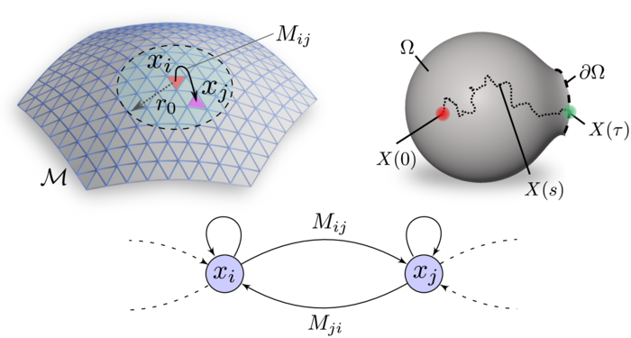
Figure 1: Markov-Chain Discretization of Particle Drift-Diffusion on Curved Surfaces. The surface is discretized using a triangulation with random walks between centriods $x_{i}$ and $x_{j}$ having jump rates $M_{ij}$ determined by the local geometry (top-left) which can be expressed as a Markov-Chain (bottom). The Markov-Chain discretization yields a backward equation for $\Omega$ allowing readily for computation of first-passage times $\tau$ (FPTs) for reaching the boundary $\partial\Omega$ and other statistics without the need in some cases for Monte-Carlo sampling (top-right).

II.1 Particle Drift-Diffusion Dynamics

We discuss a few results related to the drift-diffusion dynamics of particles useful in developing our methods. We then approximate the particle dynamics using a Markov-Chain process [72] with jump rates based on estimating the local geometry, see Figure 1.

The drift-diffusion dynamics of a particle immersed within a viscous fluid is given by the Langevin equation [73, 74]

$$m\,\differential\mathbf{V}_{t}=-\gamma\mathbf{V}_{t}\,dt-\nabla U(\mathbf{X}_{t})\,\differential t+\sqrt{2k_{B}T\gamma}\,\differential\mathbf{W}_{t},$$ (1)

where $d\mathbf{X}_{t}=\mathbf{V}_{t}dt$. This is to be interpreted as an Itô process [75, 73]. The $\gamma$ is the drag, $U(\mathbf{x})$ is a potential energy, $k_{B}$ is Boltzmann’s constant, and $T$ is the temperature [74]. The $\differential\mathbf{W}_{t}$ are increments of the Wiener process [75, 73]. The diffusion coefficient is given by $D=k_{B}{T}/\gamma$.

We remark that in some cases the protein diffusion can also be influenced by local protein-induced deformations of the membrane [16], crowding effects (sub-super diffusive and other regimes) [76, 77], or cytoskeletal interactions [78, 24]. Our methods could be combined with such models for local deformation and crowding by augmenting the Markov-Chain jump rates. In the present work, we treat the membrane as having on average an effectively constant shape. We focus on models in the normal diffusive regime with explicit modeling of protein species, binding partners, or obstacles. We treat additional contributions through effective diffusion coefficients or in the formulated protein interaction forces.

When $m/\gamma\ll\ell^{2}/D$, where $\ell$ is the radius of the particle, the inertial contributions are negligible. In this regime, the Langevin equation can be reduced to the over-damped Smoluchowski equation

$$\differential\mathbf{X}_{t}=-\frac{1}{\gamma}\nabla U(\mathbf{X}_{t})\,\differential t+\sqrt{2D}\,\differential\mathbf{W}_{t}.$$ (2)

This can be expressed in terms of probability densities $\rho(\mathbf{x},t)$ for when $\mathbf{X}_{t}=x$. This satisfies the Fokker-Planck (FP) equation

$$\partialderivative{\rho}{t}=-\nabla\cdot\mathbf{J},\;\;\;\;\;\;\mathbf{J}=\left(-\frac{1}{\gamma}\nabla U\right)\rho-D\nabla\rho.$$ (3)

When $U=0$, this has the well-known Green’s Function for Euclidean space

$$K(\mathbf{x}^{\prime},\mathbf{x};t)=\frac{1}{(4\pi Dt)^{d/2}}\exp\left(-\frac{(\mathbf{x}^{\prime}-\mathbf{x})^{2}}{4Dt}\right).$$ (4)

From the FP equation, the $K(\mathbf{x}^{\prime},\mathbf{x};t)$ has the interpretation of the probability of a particle starting with $\mathbf{X}_{0}=\mathbf{x}$ and diffusing to location $\mathbf{X}_{t}=\mathbf{x}^{\prime}$ over the time duration $t$. We will use a related approach to determine our Markov-Chain jump rates. The FP equation has a steady-state $\rho^{*}$ with detailed balance if

$$\mathbf{J}[\rho^{*}]=-\gamma^{-1}\nabla U\rho^{*}-D\nabla\rho^{*}=0.$$ (5)

For a smooth $U(x)$ with a sufficient growth rate as $|x|\rightarrow\infty$, the FP equation has steady-state with detailed-balance for the distribution

$$\rho^{*}(\mathbf{x})=\frac{1}{Z}\exp\left(-\frac{U(x)}{kT}\right).$$ (6)

This is the Gibbs-Boltzmann distribution, and $Z$ is the partition function normalizing this to be a probability density [74].

II.2 Markov-Chain Discretization for Particle Drift-Diffusion Dynamics on Curved Surfaces

We model the drift-diffusion dynamics of individual particles on curved surfaces using discrete Markov-Chains with the jump rates based on the local geometry. The surface is discretized into a triangulated mesh and each particle is tracked by the triangle which it occupies. We use that the surface metric is induced by the surrounding embedding space [79, 80]. We use for the local jump rates

$$M_{ij}=C_{i}\exp\left(-\frac{|x_{i}-x_{j}|^{2}}{\epsilon^{2}}\right).$$ (7)

To approximate the diffusion over the time-scale $\Delta{t}$ on the surface $\mathcal{M}$, we use $\epsilon=\sqrt{4D\Delta{t}}$. The $x_{i}\in\mathcal{M}$ are the centers of the surface triangulation. The $C_{i}$ denotes the normalization constant when summing over index $j$ ensuring that $M$ is a right stochastic matrix [72].

We remark in our methods the approach of using the induced metric from the embedding allows for capturing the geometric contributions while avoiding the potentially cumbersome expressions that can arise from a more explicit treatment using differential geometry. Our methods utilize that the distances between points on the surface correspond to the arc-length determined by the path as measured using the embedding space and its associated notion of distance. As a result, in our methods the discretized surface inherits its metric without the need for further analytic derivations. Further properties of our methods include that the discretizations for curved surfaces are based on Markov-Chain transitions and as a consequence will have mass conservation up to numerical round-off errors.

The kernel $M_{ij}$ has been shown in the limit of refining the surface sampling to approximate diffusion under the surface Laplace-Beltrami operator $D\Delta_{\mathcal{M}}$ [81, 82]. This has been shown to have the accuracy

$$\begin{split}\lim_{N\to\infty}\sum_{j=1}^{N}(M_{ij}-I_{ij})u_{j}=\frac{\varepsilon^{2}}{4}\Delta_{\mathcal{M}}u(x_{i})+\mathcal{O}\left(\frac{1}{N^{1/2}},\varepsilon^{4}\right).\end{split}$$ (8)

The $\mathcal{O}$ holds with $\epsilon\rightarrow 0$. The $N$ is the number of points sampling $\mathcal{M}$ subject to a uniformity condition [81, 82, 42]. The $u_{j}=u(x_{j})$ samples a smooth test function $u$. Intuitively, this follows since the stochastic matrix $M$ converges to the operator as $\exp(\varepsilon^{2}\Delta_{\mathcal{M}}/4)=\exp(D\Delta{t}\Delta_{\mathcal{M}})\simeq\exp(D\Delta{t}\Delta)$ and $\exp(D\Delta{t}\Delta_{\mathcal{M}})\simeq I+D\Delta{t}\Delta_{\mathcal{M}}\simeq I+D\Delta{t}\Delta$, where $\Delta=\nabla\cdot\nabla$ is the standard Laplacian. The last two terms are motivated by the Taylor expansions of the exponential and the geometric terms as $\epsilon\rightarrow 0$.

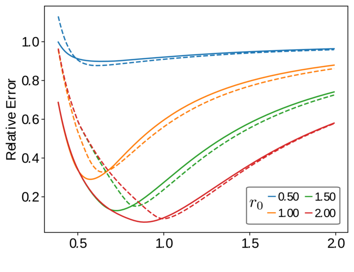
Figure 2: Approximation of Laplace-Beltrami for $\epsilon$ and $r_{0}$. Shown is the relative error of the Markov-Chain surface discretization compared with the Laplace-Beltrami operator on the unit sphere $S^{2}$. The case without area correction in equation (10) are shown as solid lines and with the area correction with dotted lines. There is a trade-off in $\epsilon$ to make it sufficiently large to contain enough points sampling the surface while also maintaining locality. For the truncation radius $r_{0}\geq 1.5$ the optimum is around $\epsilon\simeq 1$.

Since the the surface properties will only be approximated when there are a sufficient number of sample points in the support of the kernel, for a given $N$ there is a trade-off in the choice of $\epsilon$. If $\epsilon$ is too large the approximation will not be of local surface properties. If $\epsilon$ is too small only the center point will contribute significantly to the kernel. We investigate further this trade-off in $\epsilon$ and the resulting approximation accuracy in Section II.5.

We remark that our approach can also readily be modified to obtain models for proteins in super-sub diffusive regimes. One way this can be accomplished is by constructing random walks that are non-local on the mesh having long-tails or making state transitions between additional non-spatial states. These models could be constructed from theoretical considerations or empirical observations of autocorrelation statistics [76].

II.3 Detailed Balance and Area Corrections

To incorporate the contributions of the drift arising from $U$ in equation (1), we consider the Gibbs-Boltzmann distribution expressed as $\rho(x)={Z}^{-1}\exp\left(-\beta U(x)\right)$, with $\beta=(k_{B}{T})^{-1}$ the inverse thermal energy. We seek discretizations preserving statistical structure, such as detailed-balance as in  [83, 84]. For our curved surfaces, we seek discretizations for methods that have at steady-state the surface Gibbs-Boltzmann distribution with detailed balance [74]. We can express the evolution of the discrete probability in terms of net fluxes as

$$\begin{split}p_{i}^{(n+1)}=p_{i}^{(n)}+\sum_{j,j\neq i}J_{ij}^{(n)},\hskip 11.38092ptJ_{ij}^{(n)}=p_{j}^{(n)}M_{ji}-p_{i}^{(n)}M_{ij}.\end{split}$$ (9)

At steady-state $p_{k}^{(n+1)}=p_{k}^{(n)}=p_{k}^{*}$ we design our transition rates so that the we have a discrete surface Gibbs-Boltzmann distribution with approximate detailed balance. The discrete detailed-balance $J_{ij}=0$ gives the conditions

$$p_{i}^{*}=\exp\left(-\beta U_{i}\right)A_{i}/Z,\hskip 2.84544pt\frac{M_{ij}}{M_{ji}}=\frac{p_{j}^{*}}{p_{i}^{*}}=\frac{\exp\left(-\beta U_{j}\right)A_{j}}{\exp\left(-\beta U_{i}\right)A_{i}},$$ (10)

where $U_{k}=U(x_{k})$ and $Z=\sum_{i}\exp\left(-\beta U_{i}\right)A_{i}$.

Motivated by these conditions, we discretize using the transition rates

$$\begin{split}M_{ij}&=C_{i}\exp\left(-\frac{|x_{i}-x_{j}|^{2}}{\varepsilon^{2}}\right)\times\exp\left(\frac{U(x_{i})-U(x_{j})}{2k_{B}T}\right)\\ &\times\exp\left(\frac{1}{2}\ln\frac{A_{j}}{A_{i}}\right),\end{split}$$ (11)

where $C_{i}$ normalizes the $M_{ij}$ to be a probability when summing over the index $j$. The conditions hold up to the normalization ratio $C_{i}/C_{j}\rightarrow 1$ as the discretization is refined with $N\rightarrow\infty$, $\epsilon\rightarrow 0$.

Algorithm 1 Hybrid Reaction-Diffusion Method

$X_{i}^{0}\leftarrow$ initialize particle positions.

$S_{i}^{0}\leftarrow$ initialize particle states.

$q^{0}\leftarrow$ initialize fields.

$n\leftarrow 0$.

while n $<$ numsteps do

$\triangleright$ Update particles using jump rates from Section II.3.

   $X_{i}^{n+1}\leftarrow x_{b}$, $\Pr{X_{i}^{n+1}=x_{b}|X_{i}^{n}=x_{a}}=M_{ba}(q^{n},\{S_{k}^{n}\})$.

$\triangleright$ Check for chemical reactions $\mathcal{C}$ and update the states.

   $S_{i}^{n+1}\leftarrow s_{a}$, $\Pr{S_{i}^{n+1}=s_{a}|X_{i}^{n+1}=x_{b},\{X_{k}^{n}\}_{k\neq i},\{S_{k}^{n}\}}$.

$\triangleright$ Update the fields.

   $q^{n+1}\leftarrow\Psi(q^{n})$.

   n $\leftarrow$ n + 1.

end while

II.4 Chemical Reactions and Field Coupling

We also formulate methods for capturing chemical reactions. We introduce for each particle $X_{i}(t)$ an associated ”state” variable $S_{i}(t)$. The $S_{i}(t)$ can be thought of tracking the chemical species to which $X_{i}$ belongs at time $t$. We consider a collection of chemical reactions $\mathcal{C}=\{c_{\ell}\}_{\ell=1}^{m}$. For $c_{\ell}$ we model the reaction using a Smoluchowski reaction radius $r_{\ell}$ and probability $p_{\ell}$. For a second-order reaction, this means if two particles $X_{i}^{n}$ and $X_{j}^{n}$ have $\|X_{i}^{n}-X_{j}^{n}\|<r_{\ell}$, then we take probability $p_{\ell}$ for a reaction to occur. For first-order reactions, we just take $p_{\ell}=p_{\ell}(\Delta{t})$ for each particle for the probability a reaction occurs over the time-step.

We also allow for coupling of the particles to underlying fields $q=q(\mathbf{x},t)$. We discretize $q$ in time and space using the lattice with $q_{a}^{n}\sim q(\mathbf{x}_{a},t_{n})$. As we discuss in later sections, the fields can influence the local jump rates and reactions. The evolution of the field is modeled using $q^{n+1}=\Psi(q^{n})$. The case of multiple fields can be handled by taking $q$ to be vector-valued. We shall discuss in more detail specific evolution models for concentration fields in Section III.1 and phase-fields in Section III.2. We give a summary of the steps in our method in Algorithm 1.

II.5 Approximation Errors

To obtain accurate diffusive dynamics we consider how parameter choices influence the jump rates and the approximation of the Laplace-Beltrami operator discussed in Section II.3. We investigate the accuracy of the surface discretizations and the trade-offs in the choice of $\epsilon$ between sufficient sampling and maintaining locality. We perform our studies for the surface of the unit sphere $S^{2}$, which has the Laplace-Beltrami operator $\Delta_{\mathcal{M}}$ with eigenfunctions corresponding to the spherical harmonics [85, 86, 80]. In the comparisons, our numerical operator $M$ is obtained from equation (11) and the scalings indicated in (8) to yield the approximation $L=(M-I)\simeq(\epsilon^{2}/4)\Delta_{\mathcal{M}}$. In practice for efficient calculations, the $M_{ij}$ is constructed by truncating the kernel only to use neighbors $x_{j}$ within the distance $r_{0}$ with $|x_{i}-x_{j}|<r_{0}$. We consider the errors for a test function $v$ given by

$$e_{\text{LB}}[v]=\left(\frac{4}{\epsilon^{2}}\left(M-I\right)-\Delta_{S^{2}}\right)v.$$ (12)

In Figure 2, we show the relative errors based on $\epsilon_{rel}=\|e_{\text{LB}}[v]\|_{1}/\|\Delta_{S^{2}}[v]\|_{1}$, where $\|\cdot\|_{1}$ is the $L^{1}$-norm averaging over the surface. We consider case when $v$ is the spherical harmonic corresponding to $v=v(x,y,z)=z$ restricted to the surface. The sphere is discretized using a triangular mesh with nearly uniform elements having $N=10,0000$ nodal points. We consider how the error varies for different choices of $\epsilon\in[0.25,2.0]$ and $r_{0}\in[0.5,2.0]$. Letting $\delta{x}=\min_{ij}|x_{i}-x_{j}|$, we find that when $\epsilon\ll\delta{x}$ there are insufficient number of points in the support of the kernel to estimate the surface geometry and the error becomes large. We find when $\epsilon\gg\delta{x}$ is large there are many points within the support of the kernel, but the area of support is not localized enough to provide a good estimate of the operator. We also show both the case with and without the area correction terms. We find for our relatively uniform triangulations these give comparable overall errors here. For our discretizations of the sphere based on $N=10,000$ points and $r_{0}\geq 1.5$, we find that the optimal choice is $\epsilon\simeq 1$, see Figure 2.

II.6 Role of Geometry in First-Passage Times and Other Statistics

We perform analysis to develop some results showing how our methods can be used for investigating the role of geometry of the first-passage times and other statistics associated with the drift-diffusion dynamics of particles on curved surfaces. Our Markov-Chain discretizations allow in some cases for computing efficiently statistics without the need to resort to Monte-Carlo sampling, provided the state space is not too large.

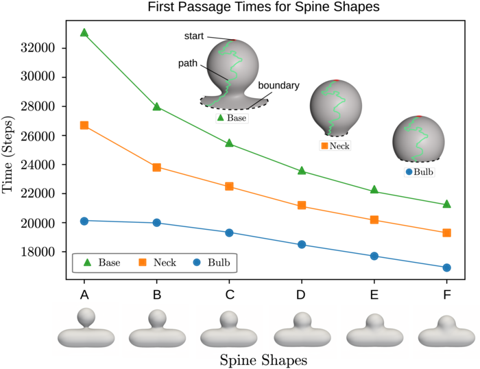
Figure 3: First-Passage Times for Spine Shapes. First passage times are computed when a protein starts at the top of the bulb-like head region and reaches the boundary. To investigate the role of the neck region verses other aspects of the shapes, three cases are considered for the boundary location, (i) at the base of the spine, (ii) in the middle of the neck, and (iii) within the spherical head region just above the neck. The results show that the neck region plays the dominant role in the geometry. As the neck narrows, the diffusion of the protein to leave the head region and enter the tubular domain has a first-passage time that significantly increases from the geometry.

We consider statistics of the form

$$u_{i}^{(n)}=\operatorname{E}\left[f(X^{(N)})+\sum_{k=n}^{N-1}g(X^{(k)},t)\;\middle|\;X^{(n)}=x_{i}\right].$$ (13)

Let $\mathbf{u}^{(k)}$ be the column vector with components $[\mathbf{u}^{(k)}]_{i}=u_{i}^{(k)}$. The $f,g:\mathcal{M}\to\mathbb{R}$ are any two smooth functions on the surface $\mathcal{M}$. Let $[\mathbf{f}]_{i}=f(x_{i})$ and $[\mathbf{g}^{(\ell)}]_{i}=g(x_{i},\ell)$ be column vectors. We also consider statistics of the form

$$w_{i}^{(\Omega)}=\operatorname{E}\left[f(X^{(\tau_{\Omega})})+\sum_{k=0}^{\tau_{\Omega}-1}g(X^{(k)})\;\middle|\;X^{(0)}=x_{i}\right].$$ (14)

For the domain $\Omega$, the $\tau_{\Omega}=\inf\{k\geq 0\;|\;X^{(k)}\not\in\Omega\}$ is the stopping time index for the process to reach the boundary $\partial\Omega$. Each of these statistics can be computed without sampling by the following results.

Theorem 1.

The statistics $\mathbf{u}^{(k)}$ of equation 13 satisfies

$$\mathbf{u}^{(n-1)} =M\mathbf{u}^{(n)}+\mathbf{g}^{(n-1)}$$ (15)

$$\mathbf{u}^{(N)} =\mathbf{f}.$$ (16)

Proof.

(see Appendix A) ∎

Theorem 2.

The statistics $\mathbf{w}^{(\Omega)}$ in equation 14 satisfies

$$(\hat{M}-\hat{I})\mathbf{w} = -\mathbf{g}$$ (17)

$$\partial{\mathbf{w}} = \mathbf{f}.$$ (18)

The $\partial{\mathbf{w}}$ extracts entries for all indices with $x_{i}\in\partial\Omega$. The $\hat{M},\hat{I}$ refers to the matrix only with the rows with indices in the interior of $\Omega$.

Proof.

(see Appendix A) ∎

In the case that $\mathbf{f}=0,\mathbf{g}=\bm{1}$, this becomes the First-Passage Time (FPT) statistic $w_{i}=\operatorname{E}[\tau_{\Omega}\;|\;X^{(0)}=x_{i}]$. These results allow for the statistics of equation 13 and 14 to be computed efficiently without the need for Monte-Carlo sampling provided the state space is not too large.

Motivated by observations that the neck geometry appears to be a strong factor in compartmentalization in dendritic spines [68, 87], we compute the first passage times of protein diffusions for different spine shapes in Figure 3. The geometries were generated from isosurfaces in a technique commonly referred to as meatballs [88]. We used several spheres to form the tubular region and another sphere for the bulb region. The geometry was obtained as the isosurface using the level set function of the form $f(x)=\sum_{k}\phi_{k}(|x-x_{k}|)$, where $\phi(r)=c_{k}/r^{2}$. The surface was triangulated at a refined spatial resolution to obtain around $N=29,000$ nodal points for each shape.

First passage times are computed for when a protein starts at the top of the head region with the bulb-like shape and reaches the boundary. To investigate the role played by the neck region compared to the influence of the other aspects of the geometry, three cases are considered for the boundary location. These are boundaries located (i) at the base of the spine, (ii) in the middle of the neck, and (iii) within the spherical head just above the neck. These results indicate that compared to the other geometric features, the width of the neck region plays the dominant role in the first passage times. As the neck narrows, the first-passage time for the protein diffusion significantly increases from these changes in the geometry, see Figure 3.

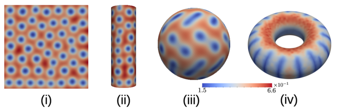
Figure 4: Role of Topology and Geometry on Pattern Formulation. The Gray-Scott reaction-diffusion shows different patterns depending on the shape of the surface. Shown are the cases of (i) square, (ii) cylinder, (iii) sphere, and (iv) torus. The surfaces have area one and when there are edges we use reflecting boundary conditions. For the shapes (i)-(ii) spotted patterns emerge having roughly a hexagonal pattern. For spherical topology (iii) a regular hexagonal pattern without defects is no longer possible, and instead striped patterns mix with spots. For the case of a torus (iv), which can sustain a hexagonal pattern in principle, the heterogeneity of the curvature appears to drive the formation of localized stripe-like patterns. These results indicate that both the geometry and topology can significantly impact pattern formation.

Parameter	Description	Value
$\epsilon_{u}$	diffusion scale for $u$	$1.0\times 10^{-2}$
$\epsilon_{v}$	diffusion scale for $v$	$5.0\times 10^{-3}$
$r_{0}$	diffusion cut-off radius	1.0
$a$	$u+2v\rightarrow 3v$ reaction rate	$4.0\times 10^{-2}$
$b$	$v\rightarrow p$ reaction rate	$6.0\times 10^{-2}$
$T_{\text{sim}}$	total time duration	$5.0\times 10^{3}$
$\Delta t$	time-step	$1.0\times 10^{-1}$
$n_{rk}$	Runge-Kutta steps	100

Table 1: Parameters for Gray-Scott Reaction-Diffusion System in Figure 4.

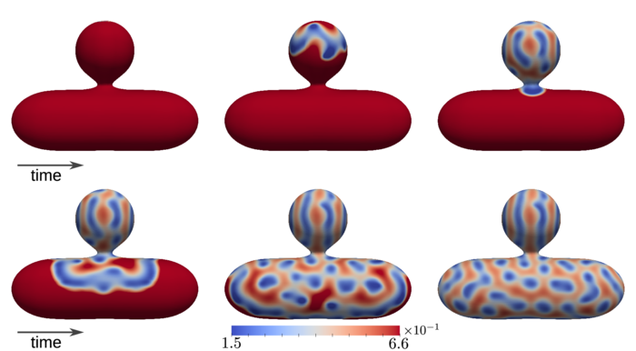
Figure 5: Evolution of Turing Instabilities for Gray-Scott Reactions. Shown is the evolution of the reaction-diffusion pattern formation process on the dendritic spine shape having the narrowest neck, label $A$ (notation the same as in Figure 3). The pattern progresses first by forming within the bulb-like head region, and then spreads through the neck to form patterning on the tubular part of the domain. The time-steps are shown for $n=0,400,800,1200,1600,2000.$

III Simulations

III.1 Turing Instabilities on Curved Surfaces

We show how our discretization approach can be used to develop methods for performing simulations of general reaction-diffusion processes on curved surfaces of different shapes. We consider reaction-diffusions, such as the pattern formation process based on Turing’s instability mechanism [89], where the geometry and topology of the domain can impact the patterns that are obtained [90, 91]. Consider the system with two molecular species with concentrations $u,v$

$$\partialderivative{u}{t}=D_{u}\Delta_{\mathcal{M}}u+f(u,v),\hskip 8.5359pt\partialderivative{v}{t}=D_{v}\Delta_{\mathcal{M}}v+g(u,v).$$ (19)

The diffusivities $D_{u}$ and $D_{v}$ will in general be different. Through the non-linear reaction terms, the difference in diffusivity can cause the homogeneously mixed concentrations to become unstable resulting in pattern generation [89, 90].

We consider Gray-Scott reactions [92], which can exhibit different patterns depending on the initial conditions and interactions with noise and other perturbations [93, 90]. For the Gray-Scott reactions [92], the terms are $f(u,v)=-uv^{2}+a(1-u)$ and $g(u,v)=uv^{2}-(a+b)v$. The rate parameters $a,b$ are for the chemical reactions $u+2v\xrightarrow[]{a}3v$ and $v\xrightarrow[]{b}p$.

Parameter	Description	Value
$\epsilon_{u}$	diffusion scale for $u$	$1.0\times 10^{-1}$
$\epsilon_{v}$	diffusion scale for $v$	$5.0\times 10^{-2}$
$r_{0}$	diffusion cut-off radius	1.0
$a$	$u+2v\rightarrow 3v$ reaction rate	$4.0\times 10^{-2}$
$b$	$v\rightarrow p$ reaction rate	$6.0\times 10^{-2}$
$T_{\text{sim}}$	total time duration	2.0
$\Delta t$	time-step	$1.0\times 10^{-3}$
$n_{rk}$	Runge-Kutta steps	1

Table 2: Parameters for Gray-Scott Reaction-Diffusion System in Figures 5 and  6.

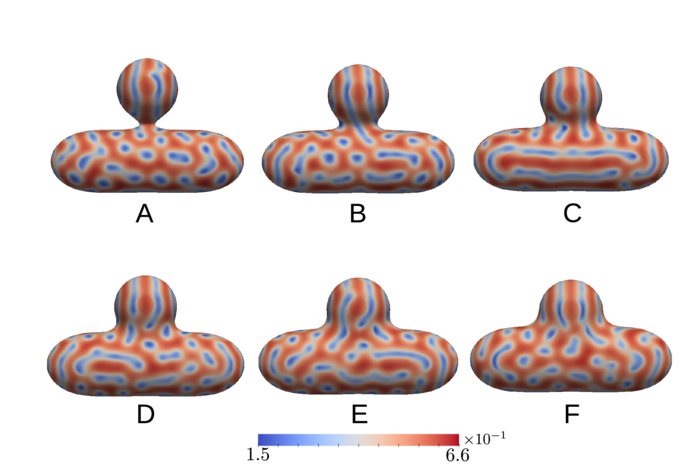
Figure 6: Gray-Scott Reaction-Diffusion Pattern Formation on Dendritic Spine Neck Shapes. Starting with the steady-state $(u^{*},v^{*})=(1,0)$, given this is stationary and the evolution is deterministic, we apply a perturbation in the shape of a circular patch on the top of the head region with the bulb-like shape with $(u,v)=(0.5\pm 10\%,0.25\pm 10\%)$. The perturbations are independent uniform variates at each lattice site. The reactions settle down into the patterns shown for time-step $2000$. Striped patterns manifest near the base of the head region and mixed spotted patterns within the tubular region.

We start with a homogeneous steady-state solution for the system $(u,v)=(1,0)$, and add small perturbations based on uniform random noise $\pm 10\%$ of the steady-state at each location $x_{i}$ within a region $\Gamma\subseteq\Omega$. Throughout our simulations, we choose $a=0.04$, $b=0.06$, guided by the parameters of the phase diagram of [94]. We investigate how the Gray-Scott patterns are influenced by different geometries and topologies.

Using our Markov-Chain discretizations, we develop numerical methods for the spatial-temporal evolution of the concentration fields. By equation (7), we obtain a stochastic matrix $M$. The overall idea is to model the concentrations by $u(x,t)=(n_{u}/A)p_{u}(x,t)$, $v(x,t)=(n_{v}/A)p_{v}(x,t)$, where $A$ is the surface area. The $\mathbf{p}=[\mathbf{p}_{u},\mathbf{p}_{v}]$, with $[\mathbf{p}^{n}]_{i}=p(x_{i},t_{n})$, are obtained from the probability evolution for the Markov-Chain given by $\mathbf{p}^{n}=\mathbf{p}^{n+1}M$. In this way, we obtain a model that approximates the diffusive evolution of the continuous concentration fields.

To model the full reaction-diffusion system in our simulations, we split the time-step integration into a diffusive step and a reaction step. For the diffusive step $\Delta{t}$, we use our Markov-Chain discretization in Section II.3 to update the concentration fields $q=(u,v)$. This provides a mean-field model for the concentration field, with $q^{n+1/2}=\Psi_{1}(q^{n})$ corresponding to $u^{n+1/2}=u^{n}M,v^{n+1/2}=v^{n}M$. The $M$ is the transition matrix for the surface diffusion derived in Section II.3. For the reactions, we use the smaller time-steps $\delta{t}=\Delta{t}/n_{rk}$ which are integrated with the fourth-order Runge-Kutta method RK4 [95, 96]. This gives $q^{n+1}=\Psi_{2}(q^{n+1/2})$. We alternate between these steps in our simulations to obtain $q^{n+1}=\Psi(q^{n})=\Psi_{2}(\Psi_{1}(q^{n}))$.

As we discussed in Section II.2, the $M$ approximates the Laplace-Beltrami operator. This ensures with enough spatial resolution the evolution will approximate diffusion on a surface. One way to view our model is as a meshfree way to discretize the surface reaction-diffusion PDEs. This provides simulation methods corresponding to the mean-field concentration fields of the protein species.

Our approaches for the diffusion also can be used more generally to go beyond the mean-field model by using discrete particle simulations with individual random walkers. These would have the same distribution as our continuum model when taking appropriate limits. Our methods allow for either (i) to perform stochastic simulations of random walks tracking individual particles to account for discrete spatial-temporal fluctuations from finite number effects, or (ii) to perform deterministic simulations tracking the probability distribution of the walkers. For the reaction-diffusion studies we use approach (ii). For later studies involving phase separation, we use approach (i).

We consider the Gray-Scott reaction-diffusion process on the following geometries (i) flat sheet with boundaries, (ii) finite cylinder with boundaries, (iii) surface of a sphere, (iv) surface of a torus, see Figure 4. The surfaces have area one and when there are boundary edges we use reflecting boundary conditions. For the shapes (i)-(ii) spotted patterns emerge having roughly a hexagonal pattern. For the spherical topology (iii) a regular hexagonal pattern without defects is no longer possible, and instead striped patterns mix with spots. For the case of a torus (iv), which can sustain a hexagonal pattern in principle, the heterogeneity of the curvature appears to drive the formation of localized stripe-like patterns. The results obtained with our methods indicate that both the geometry (curvature and scale effects) and the topology can impact significantly the pattern formation process.

We remark that Turing instabilities as a mechanism for pattern formation were originally motivated by a linear stability analysis on periodic domain performed by A. M. Turing in [89]. Extending the analysis to general manifolds is non-trivial given the challenges of analyzing even for the linearized dynamics the eigenfunctions and eigenvalues associated with the Laplace-Beltrami based-diffusions and roles of curvature and topology. Some work in this direction has been done in the literature in the case of specialized geometry, such as the sphere [97, 98]. The results of our methods for Turing instabilities yield patterns comparable to those seen in such previous studies. In the spherical case we find that there is a transition from striped to spotted patterns in the sphere size [99]. We also find that the hexagonal spotted patterns with defects manifest with arrangements similar to [97, 98].

We also consider more complicated shapes for the Gray-Scott reactions given by our mechanistic dendritic spine geometries with different neck sizes, see Figures 5, 6. These shapes consist of a bulb-like head region (representing the spine) which is connected by a neck structure to a tube-like region (representing the dendrite). We vary the shapes by changing the thickness of the neck-like structure joining the two regions. The evolution of the pattern formation process for the geometry with the narrowest and widest neck shapes are shown in Figure 5. For the narrowest necks, the confinement in the head region appears to result in stripe-like patterns that also extend through the neck. In the larger tube-like region, the spotted patterns form inter-mixed with the stripe pattern, see Figure 6. These results indicate how local regions can exhibit different patterning depending on the local geometry.

III.2 Dendritic Spines and Protein Kinetics

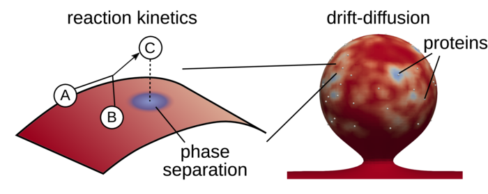
Figure 7: Chemical Kinetics and Phase Separation. We consider chemical kinetics where molecular species $A,B$ diffuse freely and react to form $C$ by $A+B\rightarrow C$. The molecular species $C$ can nucleate phase $q=-1$. The drift-diffusion of $C$ is coupled to the local phase by equation 22. This results in a bi-directional confinement force from the phase field $q$ acting on $C$ to keep within regions with $q=-1$. This also results in an equal-and-opposite force acting on the phase field from equation 22 driving nucleation and phase separation.

We develop a mechanistic model for dendritic spines to investigate the dependence of protein transport and kinetics on geometry and heterogeneities arising from phase separation. Our investigations are motivated from experiments on SynGAP and PSD-95 proteins, where phase separation may play a role in driving receptor organization [70]. Phase separation can arise from nucleation or modulating local concentrations in the cell membrane, which is a heterogeneous mixture of lipids, proteins, and other small molecules [100, 101, 1].

In our mechanistic model, we investigate how the spine geometry and phase separation can influence reaction kinetics. We start with a two species system. The $A$ and $B$ molecular species are tracked at the individual particle level. In the absence of phase separation, this would diffuse freely over the membrane surface. As a starting point, we study the basic chemical kinetics $A+B\rightarrow C$. The discrete particles react with probability $p$ when coming within a reaction distance $r<r_{0}$. This is motivated by Smoluchowski reaction kinetics [102, 103, 104, 105].

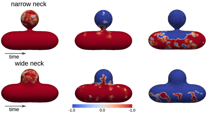
Figure 8: Dendritic Spine Model: Role of Geometry in Phase Separation. The dendritic spine model consists of a head region connected by a neck region to a tubular domain. The active proteins $A,B$ in the model all originate at the top of the head region. The phase separation occurring in the two cases is shown for (i) a narrow neck constricting the protein diffusion and spread of the phase separation (top), (ii) a wide neck through which the proteins can readily diffuse and the phase can separate (bottom). The phase $q=1$ is red and $q=-1$ is blue, shown are time-steps $50$, $300$, and $2000$. At around time-step $\sim 300$ (middle), the the protein diffusion and phase separation comes into contact with the neck region. In the narrow case, the neck region acts effectively like an entropic barrier for the diffusion arising from the geometry.

Parameter	Description	Value
$\alpha_{1}$	GL phase interfacial tension	$1.0\times 10^{6}$
$\alpha_{2}$	GL phase polarity	$1.0\times 10^{4}$
$\alpha_{3}$	GL protein-phase coupling	$1.0$
$a$	protein phase radius	$0.1$
$N$	$A$, $B$ initial protein count	1000
$\epsilon$	diffusion scale for proteins	$0.1$
$r_{0}$	diffusion cut-off radius	$0.5$
$p$	$A+B\to C$ reaction probability	$0.01$
$T_{\text{sim}}$	total time duration	$200.0$
$\Delta t$	time-step	$0.1$
$n_{rk}$	Runge-Kutta steps	$100$

Table 3: Parameters for Dendritic Spine Phase Separation.

To model such effects at a coarse-level, we track a continuum phase field $\phi=\phi(x,t)$ which can couple to the local diffusive motions of the discrete protein particles. We consider in our initial model the case of a local order parameter associated with phase separation based on Ginzburg-Landau (GL) theory [106, 107]. Other phase-separation phenomena and approaches also could be considered in principle within our framework, such as the second-order Allen-Cahn [108] or the conservative fourth-order Cahn-Hilliard [109], with additional work on the numerical methods for the operators on curved surfaces and coupling with the Markov-Chain discretization [110]. For notational convenience, we will denote $q\simeq\phi(x)$, so $q:\mathcal{M}\rightarrow\mathbb{R}$ for the phase variable map for the curved surface $\mathcal{M}$. This gives at lattice site $i$, $q_{i}\simeq\phi(x_{i})$. The GL functional is $\hat{V}_{0}[\phi]=\int_{\mathcal{M}}\left(\nabla\phi(x)\right)^{2}+\hat{V}_{2}[\phi](x)dx$. The first term accounts for a line tension between phases and the second term drives the phase to $\pm 1$ with local energy density $\hat{V}_{2}[\phi]=K(1-\phi^{2})^{2}$. To capture similar effects as $\hat{V}_{0}[q]$, we use the simplified discrete model

$$V_{0}[q]=\frac{1}{n^{2}}\sum_{i}\sum_{j\neq i}V_{1}[q_{i},q_{j}]+\frac{1}{n}\sum_{i}V_{2}[q_{i}],$$ (20)

with

$$V_{1}[q_{i},q_{j}]=\alpha_{1}W_{ij}(q_{i}-q_{j})^{2},\hskip 8.5359ptV_{2}[q]=\alpha_{2}(1-q^{2})^{2}.$$ (21)

The first term models the interfacial tension, where the coefficient $W_{ij}=W(r_{ij})$ decays in $r_{ij}=|x_{i}-x_{j}|$. The second term models the order parameter which locally is at a minimum for $q=\pm 1$. The $\alpha_{1},\alpha_{2}>0$ control the strength of the interfacial tension and the phase variable ordering. We use for the decay coefficient $W_{ij}=\exp(-r_{ij}^{2}/\varepsilon^{2})$ which is truncated for large $r_{ij}\gg\epsilon$.

To couple protein motions $\mathbf{X}(t)$ and their ability to induce local phase ordering in $q$, we use the free energy term

$$V_{3}^{(i)}[q,X]=\alpha_{3}(q_{i}-(-1))^{2}\eta_{a}(x_{i}-X).$$ (22)

The $\alpha_{3}>0$ controls the strength of this coupling. The $\eta_{a}$ gives a kernel function with support localized around the protein location $X=X(t)$. This term drives the phase field toward $q=-1$ in a region around the protein location $X(t)$. We use $\eta_{a}(r)=\exp(-r^{2}/a^{2})$ and

$$V_{3}[q,X]=\frac{1}{n}\sum_{i}V_{3}^{(i)}[q,X].$$ (23)

The free energy for full system $(q,X)$ with protein configuration $X$ and phase-field $q$ is

$$V[q,X]=V_{0}[q]+\sum_{k}V_{3}[q,X^{k}].$$ (24)

The discrete protein positions $[\mathbf{X}]_{k}=X^{k}$ are updated using the Markov-Chain discretization in equation (11) for the drift-diffusion dynamics. The energy for the protein configuration is given by $U(\mathbf{X})=V[q,\mathbf{X}]$. The time evolution of the phase field is given by

$$\frac{dq_{i}}{dt}=-\nabla_{q_{i}}V[q,X].$$ (25)

This is discretized and integrated over sub-time-steps $\delta{t}=\Delta{t}/n_{rk}$ using Runge-Kutta RK4 [95, 96]. Modeling the discrete system using the common free energy $V$ ensures the bi-directional coupling gives equal-and-opposite forces between the phase-field $q$ and the proteins $X$.

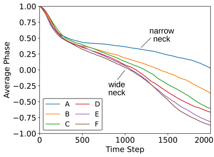
Figure 9: Dendritic Spine Model: Average Phase. The proteins $C$ can nucleate phase with $q=-1$. Shown are how the geometry impacts phase evolution for five different sizes for the neck region with labels A-F ordered from narrowest to widest as in Figure 6. The phase separation is found to slow down considerably for the narrowest neck (label A) relative to the widest neck (label F). The differences emerge around around time-step $\sim 300$, when the bulb-like head region is saturated. We see over the 2000 time-steps the widest neck results in almost the entire domain including the tubular region converting to phase $q=-1$. For the narrowest neck shape, we see at time-step $2000$ the phase separation is primarily isolated to the head head region and surrounding area, while the rest of the domain remains primarily $q=1$. The average is taken over the entire surface.

We perform simulations to investigate how the dendritic spine geometry impacts the protein reaction kinetics and phase-separation, see Figure 7 and Table 1. The proteins couple to the phase separation by having the ability to drive nucleation of local patches with $q=-1$ near the protein location $X(t)$. The geometries were chosen with the neck region taking on shapes varying from narrow to wide, see Figure 4. The protein species $A,B$ are modeled as originating in the top head region of the spine. This could arise for instance if these species correspond to tracking proteins only after they have become activated in this region. The proteins can then diffuse, and may induce local phase-separation through the coupling $V_{3}$. The proteins can also interact to form a complex which is tracked by molecular species $C$.

We show how the phase separation proceeds over time as the size of the neck region varies in Figure 8. As the neck region narrows, the protein diffusion and the phase separation are restricted to be localized in the head region. As the neck becomes wide, the protein diffusion and phase separation can readily proceed to spread more rapidly into the tubular region, see Figures 8, 9. Further effects arise from the coupling of the proteins with the local phase.

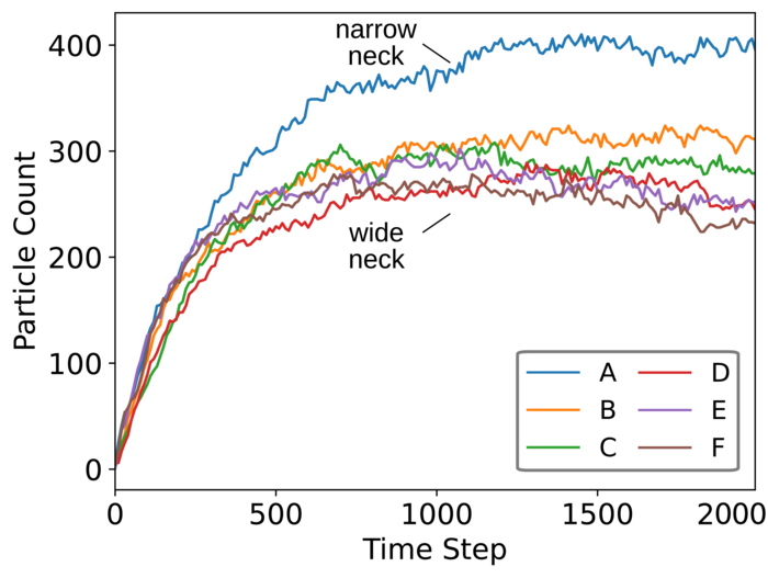
Figure 10: Dendritic Spine Model: Proteins $C$ in the Head Region. Shown are the number of proteins $C$ within the bulb-like head region over time. We see the reactions producing $C$ proceed almost independent of the geometry up to time-step $\sim 300$. Afterwards, the shapes with the narrowest necks results in far more $C$ proteins being produced and retained within the head region. This shows how phase-separation can serve to enhance retaining proteins near the top of the spine.

The protein dynamics are impacted by both the geometry and the local phase. In our simulation studies, the coupling coefficients are taken to be $\alpha_{3}^{A}=\alpha_{3}^{B}=0$ and $\alpha_{3}^{C}=1.0$. For this case $C$ can nucleate phase separation nearby since it prefers the phase field have $q=-1$. This also results for $C$ experiencing a trapping force within regions with $q=-1$, from the free energy in equation (22). This restricts the movements of $C$. The evolution of the creation of of molecular species $C$ is shown in Figure 10. The number of $C$ formed and retained in the head region is significantly impacted by the neck geometry and phase separation. When the neck is narrow, the confinement of $A,B$ and the phase separation to the head region, both enhances the creation of $C$ by more frequent $A-B$ encounters and in $C$’s retention to the head region from the phase trapping forces. As the neck becomes wide, the $A,B$ can diffuse more freely and when the phase does nucleate it can more rapidly spread throughout the whole domain. This results in a much smaller number of $C$ being created and retained in the head region.

Our basic mechanistic model shows that the morphology and phase separation can interact to serve together to enhance retaining proteins near the top of the dendritic spine. These results are expected to carry over to more complicated chemical kinetic systems. The further interactions between diffusion, kinetics, phase separation, and the geometry can regulate in different ways the spatial arrangements and the local effective rates of reactions in curved cell membranes.

III.3 Protein Clustering and Role of Phase Separation

Parameter	Description	Value
$\alpha_{1}$	GL phase interfacial tension	$1.0\times 10^{6}$
$\alpha_{2}$	GL phase polarity	$1.0\times 10^{4}$
$\alpha_{3}$	GL protein-phase coupling	0 – 10.0
$a$	protein phase radius	$0.1$
$N$	$A$, $B$ initial protein count	1000
$\epsilon$	diffusion scale for proteins	$0.1$
$r_{0}$	diffusion cut-off radius	$0.5$
$p$	$A+A\to 2A$ reaction probability	$0.001$
$q$	$A\to B$ decay probability	$0.001$
$T_{\text{sim}}$	total time duration	$200.0$
$\Delta t$	time-step	$0.1$
$n_{rk}$	Runge-Kutta steps	$100$

Table 4: Parameters for the dendritic spine phase separation simulations.

We investigate how phase separation can impact protein kinetics and clustering. Consider the case of states where proteins in state $A$ are in an active state receptive to binding and proteins in state $B$ are dormant. Consider the competing reactions for forming dimers

$$A+A\xrightarrow{p}2A,\qquad A\xrightarrow{q}B.$$ (26)

The $p$ and $q$ denote here the reaction probabilities. The protein-phase-field interactions are modeled using our approach in Section III.2. We take the phase field to impact the proteins in states $A$ and $2A$ with the same strength, $\alpha_{3}^{A}=\alpha_{3}^{2A}$. In contrast, we take proteins in the dormant state $B$ to not interact with the phase field, $\alpha_{3}^{B}=0$. To study the effects of the phase field, we vary $\alpha_{3}^{A}$ over the range from $0.0$ (no interaction) to $1\times 10^{1}$ (strong interaction). We investigate in simulations the number of dimers $2A$ proteins that are formed over time for different levels of phase field interaction $\alpha_{3}^{A}$ and as the phase separation progresses. The $2A$ counts are given in Figure 11. We find in the strongest coupling cases the phase field can significantly impact the reaction kinetics promoting clustering and dimer formation. The details of the parameters used in our simulations are given in Table 4.

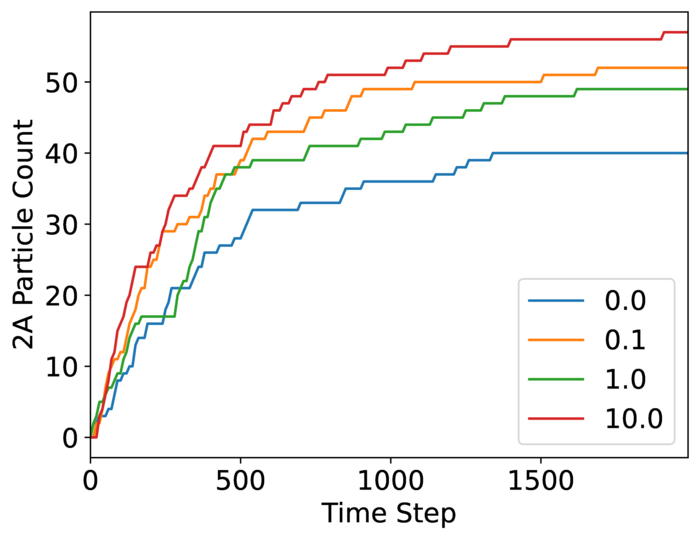
Figure 11: Dendritic Spine Model: Shown are the number of proteins $2A$ within the bulb-like head region over time. We see that increasing the interaction strength $\alpha_{3}$ (legend) between proteins $A$ and the phase field promotes the formation of clusters $2A$.

The results show that phase-field separation can play significant roles impacting reaction kinetics within membranes. In this case promoting the formation of clusters. The underlying mechanisms has to do with the formation for proteins of local environments with initially small phase-separated domains that serve to confine the diffusion of the proteins. Relative to free diffusion over the entire membrane surface, the phase confinement results in diffusion with the phase domain and more frequent encounters between co-confined proteins. In this way, the binding kinetics are enhances relative to the free diffusion. From the greater slope in the increase in the number of clusters formed for case $\alpha_{3}^{A}=1\times 10^{1}$ vs $\alpha_{3}^{A}=0$, we see the phases have the greatest impact when there are small phase domains. The smaller domains results in more frequent encounters between confined proteins. As the phase separation progresses the domains become larger and merge with the effect of the phase-coupling on the reactions become less pronounced.

These results show how phase separation and domain formation can be utilized within cell membranes to significantly augment the reaction kinetics without changing the reaction characteristics of the individual proteins. These simulation methods provide further ways to investigate the collective kinetics of proteins and the roles played by phase composition and the membrane geometry.

IV Conclusions

We have developed biophysical models for investigating protein kinetics within heterogeneous cell membranes of arbitrary shape. The introduced methods allow for studying at the continuum and discrete protein-level the drift-diffusion dynamics and reaction kinetics taking into account the roles of geometry and coupling to membrane phase separation. We have shown that coupling of kinetics to phase separation and geometry can significantly enhance or inhibit reactions and cluster formation processes. These initial results suggest a few mechanisms by which biological membranes may utilize phase separation and geometry to drive kinetics and organization of proteins within cell membranes.

V Acknowledgements

The authors P.J.A. and P.T. would like to acknowledge support for this research from the grants NSF Grant DMS-1616353 and DOE Grant ASCR PHILMS DE-SC0019246. The author T.A.B. would like to acknowledge support from grant NIH R37MH080046. P.T. would like to acknowledge a Goldwater Fellowship and College of Creative Studies Summer Undergraduate Fellowship. P.J.A. would like to acknowledge a hardware grant from Nvidia. Authors also would like to acknowledge UCSB Center for Scientific Computing NSF MRSEC (DMR1720256) and UCSB MRL NSF CNS-1725797.

Appendix A Results on Statistics of Markov-Chains and Backward Equations

We discretize the particle drift-diffusion dynamics on the surface using a Markov-Chain with jump rates $M_{ij}$. The First Passage Time (FPT) and other statistics can be computed efficiently from the Markov-Chain without the need for Monte-Carlo sampling when the discrete state space is not too large. We show how results similar to the Backward-Kolmogorov PDEs [75] can be obtained for our discrete Markov-Chains.

Theorem 1.

Let $\mathbf{u}$ be a column vector with components in $i$ associated with the statistics

$$u_{i}^{(n)}=\operatorname{E}\left[f(X^{(N)})+\sum_{t=n}^{N-1}g(X^{(t)},t)\ \biggr{\rvert}\ X^{(n)}=x_{i}\right].$$ (27)

The statistics $\mathbf{u}^{(k)}$ satisfy

$$\mathbf{u}^{(n-1)} =M\mathbf{u}^{(n)}+\mathbf{g}^{(n-1)}$$ (28)

$$\mathbf{u}^{(N)} =\mathbf{f}.$$ (29)

The $M$ is the right-stochastic matrix of the Markov-Chain. For a given choice of functions $f,g$, we collect the values $[\mathbf{f}]_{i}=f(\mathbf{x}_{i})$ and $[\mathbf{g}^{(\ell)}]_{i}=g(\mathbf{x}_{i},\ell)$ as column vectors $\mathbf{f},\mathbf{g}^{(\ell)}$.

Proof.

For the initial condition $X^{(n)}=x_{i}$, let the matrix $P^{(m)}$ have the components $P_{ij}^{(m)}=p_{j}^{(m)}$. For $m\geq n$, the $p_{j}^{(m)}$ is the solution of $\mathbf{p}^{(\ell+1)}=\mathbf{p}^{(\ell)}M$, starting with $p_{j}^{(n)}=[\mathbf{p}]_{j}^{(n)}=\delta_{ij}$. The $\delta_{ij}$ is the Kronecker $\delta$-function. For $m=n$, we have $P_{ij}^{(n)}=\delta_{ij}$. This gives

$$\begin{split}u_{i}^{(n)}&=\operatorname{E}\left[f(X^{(N)})+\sum_{t=n}^{N-1}g(X^{(t)},t)\ \biggr{\rvert}\ X^{(n)}=x_{i}\right]\\ &=\sum_{j}P^{(N)}_{ij}f(x_{j})+\sum_{t=n}^{N-1}\sum_{j}P_{ij}^{(t)}g(x_{j},t)\\ &=\sum_{j}\sum_{k}P^{(n)}_{ik}(M^{N-n})_{kj}f(x_{j})\\ &\qquad+\sum_{t=n}^{N-1}\sum_{j}\sum_{k}P_{ik}^{(n)}(M^{t-n})_{kj}g(x_{j},t)\\ &=\sum_{j}(M^{N-n})_{ij}f(x_{j})+\sum_{t=n}^{N-1}\sum_{j}(M^{t-n})_{ij}g(x_{j},t)\\ &=\left[M^{N-n}\mathbf{f}+\sum_{t=n}^{N-1}M^{t-n}\mathbf{g}^{(t)}\right]_{i}\\ &=\left[M\mathbf{u}^{(n+1)}+\mathbf{g}^{(n)}\right]_{i}.\end{split}$$ (30)

At time $t=N$, only the term with $f$ contributes and we obtain $u_{i}^{(N)}=[\mathbf{f}]_{i}$.

∎

Theorem 2.

Let $\mathbf{w}$ be a column vector with components associated with the first-passage-time statistics

$$w_{i}\equiv\operatorname{E}\left[f(X^{(\tau_{\Omega})})+\sum_{t=0}^{\tau_{\Omega}-1}g(X^{(t)})\ \biggr{\rvert}\ X^{(0)}=x_{i}\right],$$ (31)

where $\tau_{\Omega}=\inf\{k\geq 0\ |\ X^{(k)}\notin\Omega\}$. The $\mathbf{w}$ satisfies the linear equation

$$(\hat{M}-\hat{I})\mathbf{w} =-\mathbf{g}$$ (32)

$$\partial\mathbf{w} =\mathbf{f}.$$ (33)

The $\partial{\mathbf{w}}$ extracts entries for all indices with $x_{i}\in\partial\Omega$. The $\hat{M}$ refers to the rows with indices in the interior of $\Omega$.

Proof.

Since the equation is linear, we will first consider the case with $\mathbf{f}=0,\mathbf{g}\neq 0$ and then the case with $\mathbf{f}\neq 0,\mathbf{g}=0$. The general solution is then the sum of these two cases. For the case with $\mathbf{f}=0,\mathbf{g}\neq 0$ we have

$$\begin{split}w_{i}&=\operatorname{E}\left[\sum_{t=0}^{\tau-1}g(X^{(t)})\ \biggr{\rvert}\ X^{(0)}=x_{i}\right]\\ &=\sum_{n=0}^{\infty}\operatorname{E}\left[\sum_{t=0}^{n-1}g(X^{(t)})\ \biggr{\rvert}\ X^{(0)}=x_{i},\tau=n\right]\Pr\{\tau=n\}\\ &=\sum_{n=0}^{\infty}g(x_{i})\Pr\{\tau=n\}\\ &\quad+\sum_{n=0}^{\infty}\sum_{x_{j}\in\Omega}\Pr\{X^{(1)}=x_{j}\ |\ X^{(0)}=x_{i}\}\Pr\{\tau=n\}\\ &\qquad\times\operatorname{E}\left[\sum_{t=1}^{n-1}g(X^{(t)})\ \biggr{\rvert}\ X^{(0)}=x_{i},X^{(1)}=x_{j},\tau=n\right]\\ &=g(x_{i})+\sum_{x_{j}\in\Omega}M_{ij}\sum_{n=0}^{\infty}\Pr\{\tau=n\}\\ &\quad\times\operatorname{E}\left[\sum_{t=1}^{n-1}g(X^{(t)})\ \biggr{\rvert}\ X^{(0)}=x_{i},X^{(1)}=x_{j},\tau=n\right]\\ &=g(x_{i})+\sum_{x_{j}\in\Omega}M_{ij}w_{j}.\end{split}$$ (34)

In matrix form,

$$\hat{\mathbf{w}}=\mathbf{g}+\hat{M}\mathbf{w},$$ (35)

where $\hat{w},\hat{M}$ refers to the entries in the rows with indices of points in the interior of the domain $\Omega$. This can be expressed as

$$(\hat{M}-\hat{I})\mathbf{w}=-\mathbf{g}.$$ (36)

The $\hat{I}$ is the linear map that extracts entries within the interior of the domain $\Omega$.

We next consider the case with $\mathbf{f}\neq 0$ and $\mathbf{g}=0$. Similarly, this follows from

$$\begin{split}w_{i}&=\operatorname{E}\left[f(X^{(\tau)})\ \biggr{\rvert}\ X^{(0)}=x_{i}\right]\\ &=\sum_{n=0}^{\infty}\operatorname{E}\left[f(X^{(n)})\ \biggr{\rvert}\ X^{(0)}=x_{i},\tau=n\right]\Pr\{\tau=n\}\\ &=\sum_{n=0}^{\infty}\sum_{x_{j}\in\Omega}\Pr\{X^{(1)}=x_{j}\ |\ X^{(0)}=x_{i}\}\Pr\{\tau=n\}\\ &\qquad\times\operatorname{E}\left[f(X^{(n)})\ \biggr{\rvert}\ X^{(0)}=x_{i},X^{(1)}=x_{j},\tau=n\right]\\ &=\sum_{x_{j}\in\Omega}M_{ij}\sum_{n=0}^{\infty}\Pr\{\tau=n\}\\ &\quad\times\operatorname{E}\left[f(X^{(n)})\ \biggr{\rvert}\ X^{(1)}=x_{j},\tau=n\right]\\ &=\sum_{x_{j}\in\Omega}M_{ij}w_{j}.\end{split}$$ (37)

For $x_{i}\in\partial\Omega$ we have $w_{i}=\operatorname{E}\left[f(X^{(\tau)})\ \biggr{\rvert}\ X^{(0)}=x_{i}\right]=f(x_{i})$, since $\tau=0$ in this case. In matrix form this gives $\partial\mathbf{w}=\mathbf{f}$ and

$$(\hat{M}-\hat{I})\mathbf{w}=0.$$ (38)

The $\partial\mathbf{w}$ extracts the entries with indices $i$ corresponding to the boundary $\partial\Omega$. Putting both cases together we have that $\mathbf{w}$ satisfies for general $\mathbf{f},\mathbf{g}$ the linear system

$$(\hat{M}-\hat{I})\mathbf{w} = -\mathbf{g}$$

$$\partial\mathbf{w} = \mathbf{f}.$$ (39)

∎

These results provide approaches for computing efficiently the statistics $\mathbf{u}$ and $\mathbf{w}$ without the need in some cases for Monte-Carlo sampling when the state space is not too large. These results provide an analogue of the Backward-Kolmogorov PDEs in the setting of our Markov-Chain discretizations of particle drift-diffusion dynamics on curved surfaces.

References

- Alberts et al. [2014] B. Alberts, A. Johnson, J. Lewis, D. Morgan, M. C. Raff, K. Roberts, P. Walter, J. H. Wilson, and T. Hunt, Molecular biology of the cell, 6th Edition (Garland Science, 2014).
- Roux et al. [2005] A. Roux, D. Cuvelier, P. Nassoy, J. Prost, P. Bassereau, and B. Goud, The EMBO Journal 24, 1537 (2005).
- Noske et al. [2008] A. B. Noske, A. J. Costin, G. P. Morgan, and B. J. Marsh, The 4th International Conference on Electron TomographyThe 4th International Conference on Electron Tomography, Journal of Structural Biology 161, 298 (2008).
- Adler et al. [2010] J. Adler, A. Shevchuk, P. Novak, Y. Korchev, and I. Parmryd, Nat. Methods 7, 170 (2010).
- Aimon et al. [2013] S. Aimon, A. Callan-Jones, A. Berthaud, M. Pinot, G. Toombes, and P. Bassereau, Preprint 000, 0000 (2013).
- Vogel and Sheetz [2006] V. Vogel and M. Sheetz, Nat. Rev. Mol. Cell Biol. 7, 265 (2006).
- Kusters and Storm [2014] R. Kusters and C. Storm, Physical Review E 89, 032723 (2014).
- Voeltz and Prinz [2007] G. K. Voeltz and W. A. Prinz, Nat Rev Mol Cell Biol 8, 258 (2007).
- Parthasarathy and Groves [2007] R. Parthasarathy and J. T. Groves, Soft Matter 3, 24 (2007).
- Powers et al. [2002] T. R. Powers, G. Huber, and R. E. Goldstein, Phys. Rev. E 65, 041901 (2002).
- Kahraman et al. [2012] O. Kahraman, N. Stoop, and M. M. Müller, New Journal of Physics 14, 095021 (2012).
- David Nelson [2004] T. P. David Nelson, Steven Weinberg, Statistical Mechanics of Membranes and Surfaces (World Scientific Publishing, 2004).
- Saffman and Delbrück [1975] P. G. Saffman and M. Delbrück, Proc. Natl. Acad. Sci. USA 72, 3111 (1975).
- Peters and Cherry [1982] R. Peters and R. J. Cherry, Proceedings of the National Academy of Sciences 79, 4317 (1982).
- Domanov et al. [2011] Y. A. Domanov, S. Aimon, G. E. S. Toombes, M. Renner, F. Quemeneur, A. Triller, M. S. Turner, and P. Bassereau, Proc. Natl. Acad. Sci. USA 108, 12605 (2011).
- Quemeneur et al. [2014] F. Quemeneur, J. K. Sigurdsson, M. Renner, P. J. Atzberger, P. Bassereau, and D. Lacoste, Proceedings of the National Academy of Sciences 111, 5083 (2014).
- Liu et al. [2017] K. Liu, G. R. Marple, J. Allard, S. Li, S. Veerapaneni, and J. Lowengrub, Soft matter 13, 3521 (2017).
- Mahapatra et al. [2021] A. Mahapatra, D. Saintillan, and P. Rangamani, Soft Matter , (2021).
- Yushutin et al. [2019] V. Yushutin, A. Quaini, S. Majd, and M. Olshanskii, International journal for numerical methods in biomedical engineering 35, e3181 (2019).
- Pastor [1994] R. W. Pastor, Curr. Opin. Struct. Biol. 4, 486 (1994).
- Sintes and Baumgärtner [1998] T. Sintes and A. Baumgärtner, Physica A 249, 571 (1998).
- Kerr et al. [2008] R. A. Kerr, T. M. Bartol, B. Kaminsky, M. Dittrich, J.-C. J. Chang, S. B. Baden, T. J. Sejnowski, and J. R. Stiles, SIAM journal on scientific computing : a publication of the Society for Industrial and Applied Mathematics 30, 3126 (2008).
- Schöneberg et al. [2014] J. Schöneberg, A. Ullrich, and F. Noé, BMC Biophysics 7, 11 (2014).
- Kahraman et al. [2016] O. Kahraman, Y. Li, and C. A. Haselwandter, EPL (Europhysics Letters) 115, 68006 (2016).
- Mauro et al. [2014] A. J. Mauro, J. K. Sigurdsson, J. Shrake, P. J. Atzberger, and S. A. Isaacson, Journal of Computational Physics 259, 536 (2014).
- Collins et al. [2010] S. Collins, M. Stamatakis, and D. G. Vlachos, BMC Bioinformatics 11, 218 (2010).
- Sawhney and Crane [2020] R. Sawhney and K. Crane, ACM Transactions on Graphics 39 (2020).
- D. P. Tieleman and Berendsen [1997] S. J. M. D. P. Tieleman and H. J. C. Berendsen, Biochim. Biophys. Acta. 1331, 235 (1997).
- Goossens and De Winter [2018] K. Goossens and H. De Winter, J. Chem. Inf. Model. 58, 2193 (2018).
- Grouleff et al. [2015] J. Grouleff, S. J. Irudayam, K. K. Skeby, and B. Schiøtt, Biochimica et Biophysica Acta (BBA) - Biomembranes 1848, 1783 (2015), lipid-protein interactions.
- Reynwar et al. [2007] B. J. Reynwar, G. Illya, V. A. Harmandaris, M. M. Muller, K. Kremer, and M. Deserno, Nature 447, 461 (2007).
- Marrink et al. [2007] S. J. Marrink, H. J. Risselada, S. Yefimov, D. P. Tieleman, and A. H. de Vries, The Journal of Physical Chemistry B 111, 7812 (2007), pMID: 17569554, http://pubs.acs.org/doi/pdf/10.1021/jp071097f .
- Camley and Brown [2010] B. A. Camley and F. L. H. Brown, Phys. Rev. Lett. 105, 148102 (2010).
- Naji et al. [2009] A. Naji, P. J. Atzberger, and F. L. H. Brown, Phys. Rev. Lett. 102, 138102 (2009).
- Wang et al. [2013] Y. Wang, J. K. Sigurdsson, E. Brandt, and P. J. Atzberger, Phys. Rev. E 88, 023301 (2013).
- Sigurdsson et al. [2013] J. K. Sigurdsson, F. L. Brown, and P. J. Atzberger, Journal of Computational Physics 252, 65 (2013).
- Reister and Seifert [2005] E. Reister and U. Seifert, Eur. Phys. Lett. 71, 859 (2005).
- Reister-Gottfried et al. [2010] E. Reister-Gottfried, S. M. Leitenberger, and U. Seifert, Phys. Rev. E 81, 031903 (2010).
- Oppenheimer and Diamant [2009] N. Oppenheimer and H. Diamant, Biophysical Journal 96, 3041 (2009).
- Rower et al. [2019] D. Rower, M. Padidar, and P. J. Atzberger, arXiv (2019).
- Macdonald et al. [2013] C. B. Macdonald, B. Merriman, and S. J. Ruuth, Proceedings of the National Academy of Sciences 110, 9209 (2013), https://www.pnas.org/content/110/23/9209.full.pdf .
- Gross and Atzberger [2018] B. Gross and P. Atzberger, Journal of Computational Physics 371, 663 (2018).
- Lai and Li [2017] R. Lai and J. Li, SIAM Journal on Scientific Computing 39, A2231 (2017).
- Gross et al. [2021] B. J. Gross, P. Kuberry, and P. J. Atzberger, arXiv preprint arXiv:2102.02421 (2021).
- Alvarez and Sabatini [2007] V. A. Alvarez and B. L. Sabatini, Annual Review of Neuroscience 30, 79 (2007), pMID: 17280523, https://doi.org/10.1146/annurev.neuro.30.051606.094222 .
- Yuste and Denk [1995] R. Yuste and W. Denk, Nature 375, 682 (1995).
- Lu et al. [2014] H. E. Lu, H. D. MacGillavry, N. A. Frost, and T. A. Blanpied, The Journal of Neuroscience 34, 7600 (2014).
- Herring and Nicoll [2016] B. E. Herring and R. A. Nicoll, Annual Review of Physiology 78, 351 (2016), pMID: 26863325, https://doi.org/10.1146/annurev-physiol-021014-071753 .
- Nicoll [2017] R. A. Nicoll, Neuron 93, 281 (2017).
- Holcman and Schuss [2011] D. Holcman and Z. Schuss, The Journal of Mathematical Neuroscience 1, 10 (2011).
- Li et al. [2016] T. P. Li, Y. Song, H. D. MacGillavry, T. A. Blanpied, and S. Raghavachari, Journal of Neuroscience 36, 4276 (2016), https://www.jneurosci.org/content/36/15/4276.full.pdf .
- Wang et al. [2016] L. Wang, A. Dumoulin, M. Renner, A. Triller, and C. G. Specht, PLOS ONE 11, 1 (2016).
- Adrian et al. [2017] M. Adrian, R. Kusters, C. Storm, C. C. Hoogenraad, and L. C. Kapitein, Biophysical Journal 113, 2261 (2017).
- Chen and De Schutter [2017] W. Chen and E. De Schutter, Neuroinformatics 15, 1 (2017).
- Simon et al. [2014] C. Simon, I. Hepburn, W. Chen, and E. De Schutter, Journal of Computational Neuroscience 36, 483 (2014).
- Cartailler et al. [2018] J. Cartailler, T. Kwon, R. Yuste, and D. Holcman, Neuron 97, 1126 (2018).
- Cugno et al. [2019] A. Cugno, T. M. Bartol, T. J. Sejnowski, R. Iyengar, and P. Rangamani, Scientific Reports 9, 11676 (2019).
- Borczyk et al. [2019] M. Borczyk, M. A. Śliwińska, A. Caly, T. Bernas, and K. Radwanska, Scientific Reports 9, 1693 (2019).
- Tapia et al. [2019] J.-J. Tapia, A. S. Saglam, J. Czech, R. Kuczewski, T. M. Bartol, T. J. Sejnowski, and J. R. Faeder, Mcell-r: A particle-resolution network-free spatial modeling framework, in Modeling Biomolecular Site Dynamics: Methods and Protocols, edited by W. S. Hlavacek (Springer New York, New York, NY, 2019) pp. 203–229.
- Miermans et al. [2017] C. A. Miermans, R. P. T. Kusters, C. C. Hoogenraad, and C. Storm, PLOS ONE 12, 1 (2017).
- Tønnesen and Nägerl [2016] J. Tønnesen and U. V. Nägerl, Frontiers in Psychiatry 7, 101 (2016).
- Nishiyama and Yasuda [2015] J. Nishiyama and R. Yasuda, Neuron 87, 63 (2015).
- Heine et al. [2008] M. Heine, L. Groc, R. Frischknecht, J.-C. Béïque, B. Lounis, G. Rumbaugh, R. L. Huganir, L. Cognet, and D. Choquet, Science 320, 201 (2008).
- Frost et al. [2012] N. A. Frost, H. E. Lu, and T. A. Blanpied, PLoS ONE 7, e36751 (2012).
- Frost et al. [2010] N. A. Frost, H. Shroff, H. Kong, E. Betzig, and T. A. Blanpied, Neuron, Neuron 67, 86 (2010).
- Holcman and Yuste [2015] D. Holcman and R. Yuste, Nature Reviews Neuroscience 16, 685 (2015).
- Jaskolski et al. [2009] F. Jaskolski, B. Mayo-Martin, D. Jane, and J. M. Henley, Journal of Biological Chemistry 284, 12491 (2009).
- Tønnesen et al. [2014] J. Tønnesen, G. Katona, B. Rózsa, and U. V. Nägerl, Nature Neuroscience 17, 678 (2014).
- Groc and Choquet [2020] L. Groc and D. Choquet, Science 368, eaay4631 (2020), https://www.science.org/doi/pdf/10.1126/science.aay4631 .
- Zeng et al. [2016] M. Zeng, Y. Shang, Y. Araki, T. Guo, R. L. Huganir, and M. Zhang, Cell 166, 1163 (2016).
- Zeng et al. [2019] M. Zeng, J. Díaz-Alonso, F. Ye, X. Chen, J. Xu, Z. Ji, R. A. Nicoll, and M. Zhang, Neuron 104, 529 (2019).
- Ross [1996] S. M. Ross, Stochastic Processes (Wiley, 1996).
- Gardiner [1985] C. W. Gardiner, Handbook of stochastic methods, Series in Synergetics (Springer, 1985).
- Reichl [1997] L. E. Reichl, A Modern Course in Statistical Physics (Jon Wiley and Sons Inc., 1997).
- Oksendal [2000] B. Oksendal, Stochastic Differential Equations: An Introduction (Springer, 2000).
- Höfling and Franosch [2013] F. Höfling and T. Franosch, Reports on progress in physics. Physical Society (Great Britain) 76, 046602 (2013).
- Fanelli and McKane [2010] D. Fanelli and A. J. McKane, Phys. Rev. E 82, 021113 (2010).
- Takenawa and Suetsugu [2007] T. Takenawa and S. Suetsugu, Nature Reviews Molecular Cell Biology 8, 37 (2007).
- Pressley [2001] A. Pressley, Elementary Differential Geometry (Springer, 2001).
- Abraham et al. [1988] R. Abraham, J. Marsden, and T. Rațiu, Manifolds, Tensor Analysis, and Applications, v. 75 (Springer New York, 1988).
- Singer [2006] A. Singer, Applied and Computational Harmonic Analysis 21, 128 (2006), special Issue: Diffusion Maps and Wavelets.
- Belkin and Niyogi [2008] M. Belkin and P. Niyogi, Journal of Computer and System Sciences 74, 1289 (2008), learning Theory 2005.
- Latorre et al. [2011] J. C. Latorre, P. Metzner, C. Hartmann, and C. Schütte, Commun. Math. Sci. 9, 1051 (2011).
- WANG et al. [2003] H. WANG, C. S. PESKIN, and T. C. ELSTON, Journal of Theoretical Biology 221, 491 (2003).
- Müller [1966] C. Müller, Spherical Harmonics (Springer, 1966).
- Atkinson and Han [2010] K. Atkinson and W. Han, Spherical Harmonics and Approximations on the Unit Sphere: An Introduction (Springer, 2010).
- Hugel et al. [2009] S. Hugel, M. Abegg, V. de Paola, P. Caroni, B. H. Gähwiler, and R. A. McKinney, Cerebral Cortex 19, 697 (2009).
- Blinn [1982] J. F. Blinn, ACM Trans. Graph. 1, 235–256 (1982).
- Turing [1952] A. M. Turing, Philosophical Transactions of the Royal Society of London. Series B, Biological Sciences 237, 37 (1952).
- Britton [2005] N. Britton, Essential Mathematical Biology, Springer Undergraduate Mathematics Series (Springer London, 2005).
- Murray [2013] J. Murray, Mathematical Biology II: Spatial Models and Biomedical Applications, Interdisciplinary Applied Mathematics (Springer New York, 2013).
- Gray and Scott [1984] P. Gray and S. Scott, Chemical Engineering Science 39, 1087 (1984).
- Atzberger [2010] P. J. Atzberger, Journal of Computational Physics 229, 3474 (2010).
- Pearson [1993] J. E. Pearson, Science 261, 189 (1993).
- Burden and Faires [2010] R. L. Burden and D. Faires, Numerical Analysis (Brooks/Cole Cengage Learning, 2010).
- Iserles [2008] A. Iserles, A First Course in the Numerical Analysis of Differential Equations, 2nd ed., Cambridge Texts in Applied Mathematics (Cambridge University Press, 2008).
- Varea et al. [1999] C. Varea, J. L. Aragón, and R. A. Barrio, Phys. Rev. E 60, 4588 (1999).
- Jamieson-Lane et al. [2016] A. Jamieson-Lane, P. H. Trinh, and M. J. Ward, in Mathematical and computational approaches in advancing modern science and engineering (Springer, 2016) pp. 641–651.
- Hinz et al. [2019] J. Hinz, J. van Zwieten, M. Möller, and F. Vermolen, arXiv 10.48550/ARXIV.1910.12588 (2019).
- Simons and Vaz [2004] K. Simons and W. L. C. Vaz, Ann. Rev. Biophys. Biomol. Struct. 33, 269 (2004).
- Lingwood and Simons [2010] D. Lingwood and K. Simons, Science (New York, N.Y.) 327, 46 (2010).
- v. Smoluchowski [1918] M. v. Smoluchowski, Zeitschrift für Physikalische Chemie 92U, 129 (1918).
- Gillespie et al. [2013] D. T. Gillespie, A. Hellander, and L. R. Petzold, The Journal of chemical physics 138, 05B201_1 (2013).
- Isaacson [2013] S. A. Isaacson, The Journal of chemical physics 139, 054101 (2013).
- Isaacson et al. [2011] S. Isaacson, D. McQueen, and C. S. Peskin, Proceedings of the National Academy of Sciences 108, 3815 (2011).
- Hohenberg and Krekhov [2015] P. Hohenberg and A. Krekhov, Physics Reports 572, 1 (2015), an introduction to the Ginzburg–Landau theory of phase transitions and nonequilibrium patterns.
- Ginzburg and Landau [1950] V. L. Ginzburg and L. D. Landau, Zh. Eksp. Teor. Fiz. 20, 1064 (1950).
- Allen and Cahn [1979] S. M. Allen and J. W. Cahn, Acta Metallurgica 27, 1085 (1979).
- Cahn and Hilliard [1958] J. W. Cahn and J. E. Hilliard, The Journal of Chemical Physics 28, 258 (1958), https://doi.org/10.1063/1.1744102 .
- Gross et al. [2020] B. Gross, N. Trask, P. Kuberry, and P. Atzberger, Journal of Computational Physics 409, 109340 (2020).