Abstract

(1) Purpose: This work aims at developing a generalizable MRI reconstruction model in the meta-learning framework. The standard benchmarks in meta-learning are challenged by learning on diverse task distributions. The proposed network learns the regularization function in a variational model and reconstructs MR images with various under-sampling ratios or patterns that may or may not be seen in the training data by leveraging a heterogeneous dataset. (2) Methods: We propose an unrolling network induced by learnable optimization algorithms (LOA) for solving our nonconvex nonsmooth variational model for MRI reconstruction. In this model, the learnable regularization function contains a task-invariant common feature encoder and task-specific learner represented by a shallow network. To train the network we split the training data into two parts: training and validation, and introduce a bilevel optimization algorithm. The lower-level optimization trains task-invariant parameters for the feature encoder with fixed parameters of the task-specific learner on the training dataset, and the upper-level optimizes the parameters of the task-specific learner on the validation dataset. (3) Results: The PSNR increases 1.5 dB on average compared to the network trained through conventional supervised learning on the seen CS ratios. We test the result of quick adaption on the unseen tasks after meta-training, the average PSNR arises 1.22 dB compared to the conventional learning procedure that is directly trained on the unseen CS ratios in the meanwhile saving half of the training time. The average PSNR arises 1.87 dB for unseen sampling patterns comparing to conventional learning; (4) Conclusion: We proposed a meta-learning framework consisting of the base network architecture, design of regularization, and bi-level optimization-based training. The network inherits the convergence property of the LOA and interpretation of the variational model. The generalization ability is improved by the designated regularization and bilevel optimization-based training algorithm.

1 1 0 https://doi.org/ An Optimization-Based Meta-Learning Model for MRI Reconstruction with Diverse Dataset Title Wanyu Bian ^1,†,*, Yunmei Chen ¹, Xiaojing Ye², and Qingchao Zhang ¹ Wanyu Bian, Yunmei Chen, Xiaojing Ye, and Qingchao Zhang Bian, W.; Chen, Y.; Ye, X.; Zhang, Q. Correspondence: wanyu.bian@ufl.edu; Author list in alphabetical order.

1 Introduction

Deep learning models and algorithms are often built for specific tasks and the samples (usually) follow a certain distribution. Specifically, the source-domain/training samples and target-domain/testing samples are drawn from the same distribution. However, these data sets are often collected at different sources and exhibit substantial heterogeneity, and thus the samples may follow closely related but different distributions in real-world applications. Therefore, robust and efficient training of deep neural networks using such data sets is theoretically important and practically relevant in deep learning research.

Meta-learning provides an unique paradigm to overcome this challenge Munkhdalai and Yu (2017); Finn et al. (2017); Li et al. (2018); Rusu et al. (2018); Yao et al. (2021); Balaji et al. (2018). Meta-learning is known as learning-to-learn which aims to gain the capability of quickly learning unseen tasks from the experience of learning episodes that covers the distribution of relevant tasks. In a multiple-task scenario, given a family of tasks, meta-learning has been proven as a useful tool for extracting task-agnostic knowledge and improve the learning performance of new tasks from that family Thrun and Pratt (1998); Hospedales et al. (2021). Most of the modern approaches of meta-learning are focus on domain adaptation, where the target domain information is available in meta-training, but this setting is still too ideal to apply in practice. Recently the study on domain generalization (DG) has attracted much attention. DG allows the training model to learn representations from several related source domains and gain adequate generalization ability for unseen test distributions. However, DG techniques for image reconstruction are rarely explored in solving inverse problems. Leveraging large-scale heterogeneous MRI data to overcome inflated prediction performance caused by small-scale clinic datasets is of great interest for more precise, predictable, and powerful health care. For the sack of reducing scan time and improve diagnostic accuracy of MRI, the data are often acquired by using different under-sampling patterns (e.g., Cartesian mask, Radial mask, Poisson mask), under-sampling ratios, and different settings of the parameters resulting in different contrast (e.g., T1-weighted, T2-weighted, proton-density (PD), and Flair). Hence the public data are heterogeneous. This work aims at developing a generalizable MRI reconstruction method in the meta-learning framework that can leverage large-scale heterogeneous datasets to reconstruct MR images with the available small-scale dataset from specific setting of the scan.

In this work, we propose a meta-learning-based model for solving the MRI image reconstructions problem by leveraging diverse/heterogeneous dataset. Data acquisition in compressed sensing MRI (CS-MRI) with k-space (Fourier space) undersampling can be formulated as follows

$$\mathbf{y}=\mathbf{P}\mathcal{F}\mathbf{x}+\mathbf{n},$$ (1)

where $\mathbf{y}\in\mathbb{C}^{p}$ is the measured k-space data with total of $p$ sampled data points, $\mathbf{x}\in\mathbb{C}^{N\times 1}$ is unknown MR image with $N$ pixels to be reconstructed, $\mathcal{F}\in\mathbb{C}^{N\times N}$ is the 2D discrete Fourier transform (DFT) matrix, and $\mathbf{P}\in\mathbb{R}^{p\times N}$ $(p<N)$ is the binary matrix representing the sampling mask in k-space.

Reconstruction of $\mathbf{x}$ from (noisy) undersampled data $\mathbf{y}$ is an ill-posed problem. An effective strategy to elevate the ill-posedness issue is to incorporate prior information by adding a regularization term. In light of the substantial success of deep learning and the massive amount of training data available nowadays, we propose to learn the regularization term and then solve $\mathbf{x}$ from the following unconstrained optimization problem

$$\bar{\mathbf{x}}=\operatorname*{arg\,min}_{\mathbf{x}}\frac{1}{2}\|\mathbf{P}\mathcal{F}\mathbf{x}-\mathbf{y}\|^{2}+R(\mathbf{x};\Theta),$$ (2)

where $\|\cdot\|$ is the standard 2-norm of vectors, the first term in the objective function in (2) is data fidelity term that ensures consistency between the reconstructed $\mathbf{x}$ and the measured data $\mathbf{y}$, and the second term $R(\mathbf{x};\Theta)$ is the regularization term that introduces prior knowledge to the image to be reconstructed and represented by a convolutional neural network (CNN) with parameters $\Theta$ that learned from training data. We will discuss in details how this regularization is formed in Sections 3 and 4.

In this paper, we first introduce a nonconvex and nonsmooth learnable optimization algorithm (LOA) with rigorous convergence guarantees. Then we construct a deep reconstruction network by following the LOA exactly. This approach is inspired by the work Chen et al. (2020), but the LOA developed in this work is different from the one in Chen et al. (2020). Furthermore, we propose a novel MRI reconstruction model (11) with a regularization term for multi-task adaptation, which consists of a task-invariant regularization and a task-specific hyperparameter. The former extracts common prior information of images from different tasks, which learns task-invariant parameters $\theta$. The latter exploits the proper task-specific parameters (also called meta-knowledge) $\omega_{i}$ for each individual task $i$. The purpose is to increase the generalization ability of the learned regularization, so that the trained LOA-induced deep reconstruction network can perform well on both seen and unseen tasks. To train the network we split the training data into two parts: training and validation, and introduce a bilevel optimization model for learning network parameters. The lower-level optimization learns the task-invariant parameters $\theta$ of the feature encoder with fixed task-specific parameters $\omega_{i}$ on the training dataset, and the upper-level optimizes the task-specific parameters on the validation dataset. The well-trained network of seen tasks can be applied to the unseen tasks with determined $\theta$. This adaptation only needs a few iterations to update $\omega_{i}$ with a small number of training samples of unseen tasks.

As demonstrated by our numerical experiments in Section 5, our proposed framework yields much improved image qualities using diverse data sets of various undersampling trajectories and ratios for MRI image reconstruction. The underpinning theory is that an effective regularization can integrate common feature and prior information from a variety of training samples from diverse data sets, but they need to be properly weighted in the reconstruction of the image under specific sample distribution (i.e., undersampling trajectory and ratios). Our contributions can be summarized as follows:

1. LOA inspired network architecture. Our network architecture exactly follows a proposed LOA of guaranteed convergence. So the network is interpretable, parameter-efficient, stable, and generates high-quality reconstructions after proper training.

2. Design of Regularization. Unlike the existing meta-learning methods, the proposed approach of network training can learn adaptive regularizer from diverse data sets. Our adaptive regularizer consists of the task-invariant portion and the task-specific portion. The task-invariant portion aims at exploiting the common features and shared information across all involved tasks, whereas the task-specific parameters only learn the regularization weight to properly balance the data fidelity and learned regularization in individual tasks.

3. A novel bilevel network training algorithm for improving generalizability. We utilize train data and validation data for training the designed network, which follows a bilevel optimization algorithm that is trained from a heterogeneous dataset. The lower-level determines the optimal task-invariant parameters for any fixed task-specific parameters, and the upper-level optimizes the task-specific parameters on validation data so that the task-invariant parameter can be adapted to different tasks.

4. Better generalization and faster adaption. On reconstructing the under-sampled MRIs with various scanning trajectories, the network after meta-training can be directly applied to reconstruct the images sampled on multiple seen trajectories and can achieve quick adaption to the new unseen trajectories sampling patterns.

The remainder of the paper is organized as follows. In Section 2, we introduce some related work for both optimization-based meta-learning and deep unrolled networks for MRI reconstructions. We sketch our meta-learning model and the neural network in Section 3 and describe the implementation details in Section 4. Section 5 introduces the reconstruction results. Section 6 concludes the paper.

2 Related work

Meta-learning methods have in recent years yielded impressive results in various fields with different techniques, and plays a different roles in different communities, it has a very broad definition and perspective in the literature Hospedales et al. (2021). Several survey papers Hospedales et al. (2021); Huisman et al. (2021) have a detailed introduction of this development. Three categories of meta-learning techniques are commonly grouped Yao et al. (2020); Lee and Choi (2018); Huisman et al. (2021) as metric-based methods Koch et al. (2015); Vinyals et al. (2016); Snell et al. (2017), model-based methods Mishra et al. (2017); Ravi and Larochelle (2016); Qiao et al. (2018); Graves et al. (2014), and optimization-based methods Finn et al. (2017); Rajeswaran et al. (2019); Li et al. (2017), which are often cast as a bi-level optimization problem and exhibits relatively better generalizability on wider task distributions. We mainly focus on optimization-based meta-learning in this paper.

2.1 Optimization-based approaches

In the context of optimization-based meta-learning, a popular strategy is gradient descent based inner optimization Finn et al. (2017); Antoniou et al. (2018); Rajeswaran et al. (2019); Li et al. (2017); Nichol et al. (2018); Finn et al. (2019); Grant et al. (2018); Finn et al. (2018); Yoon et al. (2018). The optimization problem is often cast as a bilevel learning, where the outer level (upper/leader level) optimization is solved subject to the optimality of inner level (lower/follower level) optimization so that the optimized model can generalize well on the new data. The inner level encounters new tasks and tries to learn the associated features quickly from the training observations, the outer level accumulates task-specific meta-knowledge across previous tasks and the meta-learner provides support for the inner level so that it can quickly adapt to new tasks. e.g. the Model-Agnostic Meta-Learning (MAML) Finn et al. (2017) aims at searching for an adaptive initialization of the network parameters for new tasks with only a few steps that updates in the inner level. In recent years, a large number of followup works of MAML proposed to improve generalization using similar strategy Lee and Choi (2018); Rusu et al. (2018); Finn et al. (2018); Grant et al. (2018); Nichol et al. (2018); Vuorio et al. (2019); Yao et al. (2019); Yin et al. (2020). Deep bilevel learning Jenni and Favaro (2018) seeks to obtain better generalization that trained on one task and generalize well on another task. Their model is to optimize a regularized loss function to find network parameters from training set and identify hyperparameters so that the network performs well on validation dataset.

When the unseen tasks lie in inconsistent domains with the meta-training tasks, as revealed in Chen et al. (2019), the generalization behavior of the meta-learner will be compromised. This phenomenon partially arises from the meta-overfitting on the already seen meta-training tasks, which is identified as memorization problem in Yin et al. (2020). A meta-regularizer forked with information theory is proposed in Yin et al. (2020) to handle the memorization problem by regulating the information dependency during the task adaption. MetaReg Balaji et al. (2018) decouples the entire network into the feature network and task network, where the meta-regularization term is only applied to the task network. They first update the parameters of the task network with meta-train set to get the domain-aligned task network, then update the parameters of meta-regularization term on meta-test set to learn the cross-domain generalization. Different from MetaReg, Feature-Critic Networks Li et al. (2019) exploits the meta-regularization term to pursue a domain-invariant feature extraction network. The meta-regularization is designed as a feature-critic network that takes the extracted feature as input. The parameters of the feature extraction network are updated by minimizing the new meta-regularized loss. The auxiliary parameters in the feature-critic network are learned by maximizing the performance gain over the non-meta case. To effectively evaluate the performance of the meta-learner, several new benchmarks Rebuffi et al. (2017); Triantafillou et al. (2020); Yu et al. (2020) were developed under more realistic settings operate well on diverse visual domains. As mentioned in Triantafillou et al. (2020), the generalization to unseen tasks within multimodal or heterogeneous datasets remains as a challenge to the existing meta-learning methods.

The aforementioned methods pursue domain generalization for the classification networks that learned regularization function to learn cross-domain generalization. Our proposed method is aiming for solving the inverse problem and we construct an adaptive regularization that not only learns the universal parameters among tasks, but also the task-aware parameters. The designated adaptive regularizer assists the generalization ability of the deep model so that the well-trained model could be able to perform well on a heterogeneous datasets of both seen or unseen tasks.

2.2 MRI reconstruction models and algorithms

MRI reconstruction is generally formulated as a variation model in the format of (2), which is a data fidelity term plus a regularization term. Traditional methods employ handcrafted regularization terms such as total variation (TV), and the solution algorithm follows a theoretical justification. However, it is hard to tune the associated parameter (often require hundreds even thousands of iterations to converge) to capture subtle details and satisfy clinic diagnostic quality.

Deep learning based model leverages large dataset and further explore the potential improvement of reconstruction performance comparing to traditional methods and has successful applications in clinic field Lundervold and Lundervold (2019); Liang et al. (2020); Sandino et al. (2020); McCann et al. (2017); Zhou et al. (2020); Singha et al. (2021); Chandra et al. (2021); Ahishakiye et al. (2021). However, training generic deep neural networks (DNNs) may prone to over-fitting when data is scarce as we mentioned in the beginning. Also, the deep network structure behaves like a black box without mathematical interpretation. To improve the interpretability of the relation between the topology of the deep model and reconstruction results, a new emerging class of deep learning-based methods is known as learnable optimization algorithms (LOA) attracts attention in the literature Liu et al. (2020); Liang et al. (2020). LOA was proposed to map existing optimization algorithms to structured networks where each phase of the networks correspond to one iteration of an optimization algorithm or replace some ingredients such as proximal operator Cheng et al. (2019); Bian et al. (2020), matrix transformations Yang et al. (2018); Hammernik et al. (2018); Zhang and Ghanem (2018), non-linear operators Yang et al. (2018); Hammernik et al. (2018), and denoiser/regularizer Aggarwal et al. (2018); Schlemper et al. (2017) etc., by CNNs to avoid difficulty for solving non-smooth non-convex problems.

Different from the current LOA approach for image reconstruction that simply imitates the algorithm iterations without any convergence justification or just replaces some hardly solvable components with sub-networks, our proposed LOA-induced network inherits the convergence property of the proposed Algorithm 1, where we provide convergence analysis in Appendix A. The proposed network retains the interpretability of the variational model, parameter efficiency and contributes to better generalization.

3 Proposed Method

3.1 LOA-induced reconstruction network

Our deep algorithmic unrolling reconstruction network represented as $F_{\Theta}$ where $\Theta$ denotes the set of all learnable parameters in the model. Motivated by the variational model, for an input partial k-space data $\mathbf{y}$ in $\mathcal{D}_{\tau_{i}}$, we desire the network output $F_{\Theta}(\mathbf{y})$ to be an optimizer of the following minimization problem as (3). We use "$\approx$" since in practice we only do finite-step optimization algorithm to approximate the optimizer

$$F_{\Theta}(\mathbf{y})\approx\operatorname*{arg\,min}_{\mathbf{x}}\big{\{}\phi_{\Theta}(\mathbf{x},\mathbf{y}):=f(\mathbf{x},\mathbf{y})+R(\mathbf{x};\Theta)\big{\}},$$ (3)

where $f$ is the data fidelity term that usually takes the form $f(\mathbf{x},\mathbf{y})=\frac{1}{2}\|\mathbf{P}\mathcal{F}\mathbf{x}-\mathbf{y}\|^{2}$ in standard MRI setting, where $\mathcal{F}$ and $\mathbf{P}$ represent the Fourier transform and the binary under-sampling mask for k-space trajectory respectively. However, we remark that our approach can be directly applied to a much broader class of image reconstruction problems as long as $f$ is continuously differentiable with Lipschitz continuous gradient.

In this section, we introduce a learned optimization algorithm (LOA) for solving (3), where the network parameters $\Theta$ are learned and fixed. Since $\Theta$ are fixed in (3), we will omit them in the derivation of the LOA below and write $R(\mathbf{x};\Theta)$ as $R(\mathbf{x})$ for notation simplicity. Then we generate a multi-phase network induced by the proposed LOA, i.e. the network architecture follows the algorithm exactly such that one phase of the network is just one iteration of the LOA.

In our implementation, to incorporate sparsity along with the learned features, we parameterize the function $R(\mathbf{x})=\kappa\cdot r(\mathbf{x})$, where $\kappa>0$ is a weight parameter that needs be chosen properly depending on the specific task (e.g., noise level, undersampling ratio, etc.), and $r$ is a regularizer parameterized as a (composition of) neural networks and can be adapted to a broad range of imaging applications. In this work, we parameterize $r$ as the composition of the $l_{2,1}$ norm and a learnable feature extraction operator $\mathbf{g}_{j}(\mathbf{x})$. That is, we set $r$ in (3) to be

$$r(\mathbf{x}):=\|\mathbf{g}_{j}(\mathbf{x})\|_{2,1}=\sum_{j=1}^{m}\|\mathbf{g}_{j}(\mathbf{x})\|.$$ (4)

Here $\mathbf{g}_{j}(\cdot)=\mathbf{g}_{j}(\cdot;\theta)$ is parametrized as a convolutional neural network (CNN) where $\theta$ is the learned and fixed network parameter in $r(\cdot;\theta)$ as mentioned above. We also consider $\kappa$ to be learned and fixed as $\theta$ for now, and will discuss how to learn both of them in the next subsection. We use smooth activation function in $\mathbf{g}$ formulate in (19) which renders $\mathbf{g}$ a smooth but nonconvex function. Due to the nonsmooth $\|\cdot\|_{2,1}$, $r$ is therefore a nonsmooth nonconvex function.

Since the minimization problem in (3) is nonconvex and nonsmooth, we need to derive an efficient LOA to solve it. This solver will be termed as $F_{\Theta}(\mathbf{y})$. Here we first consider smoothing the $l_{2,1}$ norm that for any fixed $\mathbf{g}(\mathbf{x})$:

$$r_{\varepsilon}(\mathbf{x})=\sum\nolimits^{m}_{j=1}\sqrt{\|\mathbf{g}_{j}(\mathbf{x})\|^{2}+\varepsilon^{2}}-\varepsilon.$$ (5)

We denote $R_{\varepsilon}=\kappa\cdot r_{\varepsilon}$. The LOA derived here is inspired by the proximal gradient descent algorithm and iterates the following steps to solve the smoothed problem:

$$\mathbf{z}_{t+1} =\mathbf{x}_{t}-\alpha_{t}\nabla f(\mathbf{x}_{t})$$ (6a)

$$\mathbf{x}_{t+1} =\operatorname{\mathrm{prox}}_{\alpha_{t}R_{\varepsilon_{t}}}(\mathbf{z}_{t+1}),$$ (6b)

where $\varepsilon_{t}$ denotes the smoothing parameter $\varepsilon$ at the specific iteration $t$, and proximal operator is defined as $\operatorname{\mathrm{prox}}_{\alpha g}(\mathbf{b}):=\operatorname*{arg\,min}_{\mathbf{x}}\left\|\mathbf{x}-\mathbf{b}\right\|+\alpha g(\mathbf{x})$ in (6b). A quick observation from (5) is that $R_{\varepsilon}\rightarrow R$ as $\varepsilon$ diminishes, so later we will intentionally push $\varepsilon_{t}\rightarrow 0$ at Line 16 in Algorithm 1. Then one can readily show that $R_{\varepsilon}(x)\leq R(x)\leq R_{\varepsilon}(x)+\varepsilon$ for all $x$ and $\varepsilon>0$. From Algorithm 1, line 16 will automatically reduce $\varepsilon$ and the iterates will converge to the solution of the original nonsmooth nonconvex problem (3), a rigorous sense will be made precisely in the convergence analysis in Appendix A.

Since $R_{\varepsilon_{t}}$ is a complex function involving a deep neural network, its proximal operator does not have close-form and cannot be computed easily in the subproblem in (6b). To overcome this difficulty, we consider to approximate $R_{\varepsilon_{t}}$ by

$$\hat{R}_{\varepsilon_{t}}(\mathbf{z}_{t+1}) =R_{\varepsilon_{t}}(\mathbf{z}_{t+1})+\langle\nabla R_{\varepsilon_{t}}(\mathbf{z}_{t+1}),\mathbf{x}-\mathbf{z}_{t+1}\rangle+\frac{1}{\beta_{t}}\lVert\mathbf{x}-\mathbf{z}_{t+1}\rVert^{2}.$$

Then we update $\mathbf{u}_{t+1}=\operatorname{\mathrm{prox}}_{\alpha_{t}\hat{R}_{\varepsilon_{t}}}(\mathbf{z}_{t+1})$ to replace (6b), therefore we obtain

$$\mathbf{u}_{t+1}=\mathbf{z}_{t+1}-\tau_{t}\nabla R_{\varepsilon_{t}}(\mathbf{z}_{t+1}),\text{ where }\tau_{t}=\frac{\alpha_{t}\beta_{t}}{\alpha_{t}+\beta_{t}}.$$ (8)

In order to guarantee the convergence of the algorithm, we introduce the standard gradient descent of $\phi_{\varepsilon_{t}}$ (where $\phi_{\varepsilon_{t}}:=f+R_{\varepsilon_{t}}$) at $\mathbf{x}$:

$$\mathbf{v}_{t+1}=\operatorname*{arg\,min}_{\mathbf{x}}\langle\nabla f(\mathbf{x}_{t}),\mathbf{x}-\mathbf{x}_{t}\rangle+\langle\nabla R_{\varepsilon}(\mathbf{x}_{t}),\mathbf{x}-\mathbf{x}_{t}\rangle+\frac{1}{2\alpha_{t}}\|\mathbf{x}-\mathbf{x}_{t}\|^{2},$$ (9)

which yields

$$\mathbf{v}_{t+1}=\mathbf{x}_{t}-\alpha_{t}\nabla\phi_{\varepsilon_{t}}(\mathbf{x}_{t}),$$ (10)

to serve as a safeguard for the convergence. Specifically, we set $\mathbf{x}_{t+1}=\mathbf{u}_{t+1}$ if $\phi_{\varepsilon_{t}}(\mathbf{u}_{t+1})\leq\phi_{\varepsilon_{t}}(\mathbf{v}_{t+1})$; otherwise we set $\mathbf{x}_{t+1}=\mathbf{v}_{t+1}$. Then we repeat this process.

Our algorithm is summarized in Algorithm 1. The prior term with unknown parameters has the exact residual update itself which makes the training process more fluent He et al. (2016). The condition checking in Line 5 is introduced to make sure that it is in the energy descending direction. Once the condition in Line 5 fails, it comes to $\mathbf{v}_{t+1}$ and the line search in Line 12 guarantees the appropriate step size can be achieved within finite steps to make the function value decrease. From Line 3 to Line 14, we can regard that it solves a problem of minimizing $\phi_{\varepsilon_{t}}$ with $\varepsilon_{t}$ fixed. Line 15 is to update the value of $\varepsilon_{t}$ depending on a reduction criterion. The detailed analysis of this mechanism and in-depth convergence justification is shown in Appendix A. The corresponding unrolling network exactly follows the Algorithm 1, thus shares the same convergence property. Compared to LDA Chen et al. (2020) computes both candidates $\mathbf{u}_{t+1}$, $\mathbf{v}_{t+1}$ at every iteration and then chooses the one that achieves a smaller function value, we propose the criteria above in Line 5 for updating $\mathbf{x}_{t+1}$, which potentially saves extra computational time for calculating the candidate $\mathbf{v}_{t+1}$ and potentially mitigates the frequent alternations between the two candidates. Besides, the smoothing method proposed in this work is more straightforward than smoothing in dual space Chen et al. (2020) whereas still keeping provable convergence as shown in Theorem A.

The proposed LOA-induced network is a multi-phase network whose architecture exactly follows the proposed LOA 1 in the way that each phase corresponding to one iteration of the algorithm with shared parameters. These unknown parameters are trained by the method in the next section.

1:  Input: Initial $\mathbf{x}_{0}$, $0<\rho,\gamma<1$, and $\varepsilon_{0}$, $a,\sigma>0$. Max total phases $T$ or tolerance $\epsilon_{\mathrm{tol}}>0$.

2:  for $t=0,1,2,\dots,T-1$ do

3:     $\mathbf{z}_{t+1}=\mathbf{x}_{t}-\alpha_{t}\nabla f(\mathbf{x}_{t})$

4:     $\mathbf{u}_{t+1}=\mathbf{z}_{t+1}-\tau_{t}\nabla R_{\varepsilon_{t}}(\mathbf{z}_{t+1})$,

5:     if  $\|\nabla\phi_{\varepsilon_{t}}(\mathbf{x}_{t})\|\leq a\|\mathbf{u}_{t+1}-\mathbf{x}_{t}\|\ \mbox{and}\ \phi_{\varepsilon_{t}}(\mathbf{u}_{t+1})-\phi_{\varepsilon_{t}}(\mathbf{x}_{t})\leq-\frac{1}{a}\|\mathbf{u}_{t+1}-\mathbf{x}_{t}\|^{2}$ holds then

6:        set $\mathbf{x}_{t+1}=\mathbf{u}_{t+1}$,

7:     else

8:        $\mathbf{v}_{t+1}=\mathbf{x}_{t}-\alpha_{t}\nabla\phi_{\varepsilon_{t}}(\mathbf{x}_{t})$,

9:        if  $\phi_{\varepsilon_{t}}(\mathbf{v}_{t+1})-\phi_{\varepsilon_{t}}(\mathbf{x}_{t})\leq-\frac{1}{a}\|\mathbf{v}_{t+1}-\mathbf{x}_{t}\|^{2}$ holds then

10:           set $\mathbf{x}_{t+1}=\mathbf{v}_{t+1}$,

11:        else

12:           update $\alpha_{t}\leftarrow\rho\alpha_{t}$, then go to 8,

13:        end if

14:     end if

15:     if $\|\nabla\phi_{\varepsilon_{t}}(\mathbf{x}_{t+1})\|<\sigma\gamma{\varepsilon_{t}}$, set $\varepsilon_{t+1}=\gamma{\varepsilon_{t}}$; otherwise, set $\varepsilon_{t+1}={\varepsilon_{t}}$.

16:     if $\sigma{\varepsilon_{t}}<\epsilon_{\mathrm{tol}}$, terminate.

17:  end for

18:  Output: $\mathbf{x}_{T}$.

Algorithm 1 Algorithmic Unrolling Method with Provable Convergence

3.2 Bilevel optimization algorithm for network training

In this section, we consider the parameter training problem of the LOA-induced network. Specifically, we develop a bilevel optimization algorithm for training our network parameters $\Theta$ from diverse data sets.

As shown in Section 3.1, we design $R(\mathbf{x};\Theta)=\kappa\cdot r(\mathbf{x};\Theta)$, where $r$ is going to be learned to capture the intrinsic property of the underlying common features across all different tasks. To account for the large variations in the diverse training/validation data sets, we introduce a task-specific parameter $\omega_{i}$ to approximate the proper $\kappa$ for the $i$th task. Specifically, for the $i$th task, the weight $\kappa$ is set to $\sigma(\omega_{i})\in(0,1)$, where $\sigma(\cdot)$ is the sigmoid function. Therefore, $\kappa=\sigma(\omega_{i})$ finds the proper weight of $r$ for the $i$-th task according to its specific sampling ratio or pattern. The parameters $\omega_{i}$ are to be optimized in conjunction with $\Theta$ through the hyperparameter tuning process below.

Suppose that we are given $\mathcal{M}$ data pairs $\{(\mathbf{y}_{m},\hat{\mathbf{x}}_{m})\}_{m=1}^{\mathcal{M}}$ for the use of training and validation where $\mathbf{y}_{m}$ is the observation, which is partial k-space data in our setting, and $\hat{\mathbf{x}}_{m}$ is the corresponding ground truth image. The data pairs are then sampled into $\mathcal{N}$ tasks $\{\mathcal{D}_{\tau_{i}}\}_{i=1}^{\mathcal{N}}$, where each $\mathcal{D}_{\tau_{i}}$ represents the collection of data pairs in the specific task $\tau_{i}$. In each task $\tau_{i}$, we further divide the data into the task-specific training set $\mathcal{D}^{tr}_{\tau_{i}}$ and validation set $\mathcal{D}^{val}_{\tau_{i}}$. Architecture of our base network exactly follows the LOA 1 developed in previous section with learnable parameters $\theta$ and a task-specific parameter $\omega_{i}$ for the $i$th task. More precisely, for one data sample denoted by $(\mathbf{y}^{(i)}_{j},\hat{\mathbf{x}}^{(i)}_{j})$ in task $\tau_{i}$ with index $j$, we propose the algorithmic unrolling network for task $\tau_{i}$ as

$$F_{\theta,\omega_{i}}(\mathbf{y}^{(i)}_{j})\approx\operatorname*{arg\,min}_{\mathbf{x}}f(\mathbf{x},\mathbf{y}^{(i)}_{j})+\sigma(\omega_{i})r(\mathbf{x};\theta),$$ (11)

$\theta$ denotes the learnable common parameters across different tasks with task-invariant representation whereas $\omega_{i}$ is a task-specific parameter for task $\tau_{i}$. Here $\omega_{i}\in\mathbb{R}$ and $\sigma$ is the sigmoid function such that $\sigma(\omega_{i})\in(0,1)$. The weight $\sigma(\omega_{i})$ represents the weight of $r$ associated with the specific task $\tau_{i}$. We denote $\omega$ to be the set $\{\omega_{i}\}_{i=1}^{\mathcal{N}}$. The detailed architecture of this network is illustrated in Section 3.1. We define the task-specific loss

$$\ell_{\tau_{i}}(\theta,\omega_{i};\mathcal{D}_{\tau_{i}})=\sum_{j=1}^{|\mathcal{D}_{\tau_{i}}|}\ell\big{(}F_{\theta,\omega_{i}}(\mathbf{y}^{(i)}_{j}),\hat{\mathbf{x}}^{(i)}_{j}\big{)},$$ (12)

where $|\mathcal{D}_{\tau_{i}}|$ represents the cardinality of $\mathcal{D}_{\tau_{i}}$ and

$$\ell\big{(}F_{\theta,\omega_{i}}(\mathbf{y}^{(i)}_{j}),\hat{\mathbf{x}}^{(i)}_{j}\big{)}:=\frac{1}{2}\|F_{\theta,\omega_{i}}(\mathbf{y}^{(i)}_{j})-\hat{\mathbf{x}}^{(i)}_{j}\|^{2}.$$ (13)

For the sake of preventing the proposed model from overfitting the training data, we introduce a novel learning framework by formulating the network training as a bilevel optimization problem to learn $\omega$ and $\theta$ in (11) as

$$\min_{\theta,\ \omega=\omega_{i\in 1:\mathcal{N}}}\quad \sum^{\mathcal{N}}_{i=1}\ell_{\tau_{i}}(\theta(\omega),\omega_{i};\mathcal{D}^{val}_{\tau_{i}})$$ (14a)

s.t. $$\theta(\omega)=\operatorname*{arg\,min}_{\theta}\sum^{\mathcal{N}}_{i=1}\ell_{\tau_{i}}(\theta,\omega_{i};\mathcal{D}^{tr}_{\tau_{i}}).$$ (14b)

In (14), the lower-level optimization learns the task-invariant parameters $\theta$ of the feature encoder with fixed task-specific parameter $\omega_{i}$ on the training dataset, and the upper-level adjusts the task-specific parameters $\{\omega_{i}\}$ so that the task-invariant parameters $\theta$ can perform robustly on validation dataset as well. For simplicity, we omit the summation and redefine $\mathcal{L}(\theta,\omega;\mathcal{D}):=\sum^{\mathcal{N}}_{i=1}\ell_{\tau_{i}}(\theta,\omega;\mathcal{D})$, then briefly rewrite (14) as

$$\min_{\theta,\omega}\mathcal{L}(\theta(\omega),\omega;\mathcal{D}^{val})\ \ \ \ \ \mbox{s.t.}\ \ \theta(\omega)=\operatorname*{arg\,min}_{\theta}\mathcal{L}(\theta,\omega;\mathcal{D}^{tr}).$$ (15)

Then we relax (15) into a single-level constrained optimization where the lower-level problem is replaced with its first-order necessary condition following Mehra and Hamm (2019):

$$\min_{\theta,\omega}\mathcal{L}(\theta,\omega;\mathcal{D}^{val})\ \ \ \ \ \mbox{s.t.}\ \ \nabla_{\theta}\mathcal{L}(\theta,\omega;\mathcal{D}^{tr})=0.$$ (16)

which can be further approximated by an unconstrained problem by a penalty term as

$$\min_{\theta,\omega}\big{\{}\widetilde{\mathcal{L}}(\theta,\omega;\mathcal{D}^{tr},\mathcal{D}^{val}):=\mathcal{L}(\theta,\omega;\mathcal{D}^{val})+\frac{\lambda}{2}\|\nabla_{\theta}\mathcal{L}(\theta,\omega;\mathcal{D}^{tr})\|^{2}\big{\}}.$$ (17)

We adopt the stochastic gradients of the loss functions on mini-batch data sets in each iteration. In our model, we need to include the data pairs of multiple tasks in one batch, therefore we propose the cross-task mini-batches when training. At each training iteration, we randomly sample the training data pairs $\mathcal{B}^{tr}_{\tau_{i}}=\{(\mathbf{y}^{(i)}_{j},\hat{\mathbf{x}}^{(i)}_{j})\in\mathcal{D}^{tr}_{\tau_{i}}\}_{j=1}^{\mathcal{J}^{tr}}$ and the validation pairs $\mathcal{B}^{val}_{\tau_{i}}=\{(\mathbf{y}^{(i)}_{j},\hat{\mathbf{x}}^{(i)}_{j})\in\mathcal{D}^{val}_{\tau_{i}}\}_{j=1}^{\mathcal{J}^{val}}$ on each task $\tau_{i}$. Then the overall training and validation mini-batchs $\mathcal{B}^{tr}$ and $\mathcal{B}^{val}$ used in every training iteration is composed of the sampled data pairs from the entire set of tasks, i.e. $\mathcal{B}^{tr}=\bigcup_{i=1}^{\mathcal{N}}\{\mathcal{B}^{tr}_{\tau_{i}}\}$ and $\mathcal{B}^{val}=\bigcup_{i=1}^{\mathcal{N}}\{\mathcal{B}^{val}_{\tau_{i}}\}$. Thus in each iteration, we have $\mathcal{N}\cdot\mathcal{J}^{tr}$ and $\mathcal{N}\cdot\mathcal{J}^{val}$ data pairs used for training and validation respectively. To solve the minimization problem (17), we utilize the stochastic mini-batch alternating direction method summarized in Algorithm 2 which is modified from Mehra and Hamm (2019). In Algorithm 2, the parameter $\delta_{tol}$ is to control the accuracy, the algorithm will terminate when $\delta\leq\delta_{tol}$. In addition, $\lambda$ is the weight for the second constraint term of (17), in the beginning, we set $\lambda$ to be small so as to achieve a quick starting convergence then gradually increase its value to emphasize the constraint.

1:  Initialize $\theta$, ${\omega}$, $\delta$, $\lambda$ and $\nu_{\delta}\in(0,1)$,  $\nu_{\lambda}>1$.

2:  while $\delta>\delta_{tol}$ do

3:     Sample cross-task training batch $\mathcal{B}^{tr}=\bigcup_{i=1}^{\mathcal{N}}\{(\mathbf{y}^{(i)}_{j},\hat{\mathbf{x}}^{(i)}_{j})\in\mathcal{D}^{tr}_{\tau_{i}}\}_{j=1:\mathcal{J}^{tr}}$

4:     Sample cross-task validation batch $\mathcal{B}^{val}=\bigcup_{i=1}^{\mathcal{N}}\{(\mathbf{y}^{(i)}_{j},\hat{\mathbf{x}}^{(i)}_{j})\in\mathcal{D}^{val}_{\tau_{i}}\}_{j=1:\mathcal{J}^{val}}$

5:     while $\|\nabla_{\theta}\widetilde{\mathcal{L}}(\theta,\omega;\mathcal{B}^{tr},\mathcal{B}^{val})\|^{2}+\|\nabla_{\omega}\widetilde{\mathcal{L}}(\theta,\omega;\mathcal{B}^{tr},\mathcal{B}^{val})\|^{2}>\delta$ do

6:        for $k=1,2,\dots,K$ (inner loop) do

7:           $\theta\leftarrow\theta-\rho_{\theta}^{k}\nabla_{\theta}\widetilde{\mathcal{L}}(\theta,\omega;\mathcal{B}^{tr},\mathcal{B}^{val})$

8:        end for

9:        $\omega\leftarrow\omega-\rho_{\omega}\nabla_{\omega}\widetilde{\mathcal{L}}(\theta,\omega;\mathcal{B}^{tr},\mathcal{B}^{val})$

10:     end while

11:     update $\delta\leftarrow\nu_{\delta}\delta$, $\ \lambda\leftarrow\nu_{\lambda}\lambda$

12:  end while

13:  output: $\theta,{\omega}$.

Algorithm 2 Stochastic mini-batch alternating direction penalty method

4 Implementation

4.1 Feature extraction operator

We set the feature extraction operator $\mathbf{g}$ to a vanilla $l$-layer CNN with the componentwise nonlinear activation function $\varphi$ and no bias, as follows:

$$\mathbf{g}(x)=\mathbf{w}_{l}*\varphi\cdots\ \varphi(\mathbf{w}_{3}*\varphi(\mathbf{w}_{2}*\varphi(\mathbf{w}_{1}*x))),$$ (18)

where $\{\mathbf{w}_{q}\}_{q=1}^{l}$ denote the convolution weights consisting of $d$ kernels with identical spatial kernel size, and $*$ denotes the convolution operation. Here $\varphi$ is constructed to be the smoothed rectified linear unit as defined below

$$\varphi(x)=\begin{cases}0,&\mbox{if}\ x\leq-\delta,\\ \frac{1}{4\delta}x^{2}+\frac{1}{2}x+\frac{\delta}{4},&\mbox{if}\ -\delta<x<\delta,\\ x,&\mbox{if}\ x\geq\delta,\end{cases}$$ (19)

where the prefixed parameter $\delta$ is set to be $0.001$ in our experiment. The default configuration of the feature extraction operator is set as follows: the feature extraction operator $\mathbf{g}$ consists of $l=3$ convolution layers and all convolutions are with $4$ kernels of spatial size $3\times 3$.

4.2 Setups

As our method introduces an algorithmic unrolling network, there exists a one-to-one correspondence between the algorithm iterations and the neural network phases (or blocks). Each phase of the forward propagation can be viewed as one algorithm iteration, which motivates us to imitate the iterating of the optimization algorithm and use a stair training strategy Chen et al. (2020). At the first stage, we start training the network parameters using 1 phase, then after the the loss converges, we add more phases (1 phase each time) then continue the training process. We repeat this procedure and stop it until the loss does not decrease any more when we add more blocks. We minimize the loss for $100$ epochs/iterations each time using the SGD-based optimizer Adam Kingma and Ba (2015) with $\beta_{1}=0.9$, $\beta_{2}=0.999$ and initial learning rate set to $10^{-3}$ as well as the mini-batch size $8$. The Xavier Initializer Glorot and Bengio (2010) is used to initialize the weights of all convolutions. The initial smoothing parameter $\varepsilon_{0}$ is set to be $0.001$ then learned together with other network parameters. The input $\mathbf{x}_{0}$ of the unrolling network is obtained by Zero-filling strategyBernstein et al. (2001). The deep unrolling network was implemented using the Tensorflow toolbox Abadi et al. (2015) in Python programming language. Our code will be publicly shared depending on acceptance.

5 Numerical Experiments

5.1 Dataset

To validate the performance of the proposed method, the data we used are from Multimodal Brain Tumor Segmentation Challenge 2018 Menze et al. (2014), in which the training dataset contains four modalities ($T1,T1_{c},T2$ and $FLAIR$) scanned from 285 patients, and the validation dataset contains images from 66 patients, each with volume size $240\times 240\times 155$. Each modality consists of two types of gliomas: 75 volumes of low-grade gliomas (LGG) and 210 volumes of high-grade gliomas (HGG). Our implementation interested in HGG MRI in two modalities: T1 and T2 images, and we choose 30 patients from each modality in the training dataset for training our network. In the validation dataset, we randomly picked 15 patients as our validation data, and 6 patients in the training dataset as testing data which are are distinct from our training set and validation set. We cropped the 2D image size to be $160\times 180$ in the center region and picked adjacent $10$ slices in the center of each volume, which results in a total of $300$ images as our training data, $150$ images in our validation data, and a total of $60$ images as testing data. The number of data mentioned here is the amount of a single task, but since we employ multi-tasks training, the total number of images in each dataset should multiply the number of tasks. For each 2D slice, we normalize the spatial intensity by dividing the maximum pixel value.

5.2 Experiment settings and Comparison results

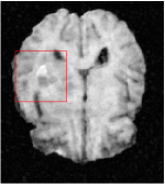
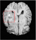
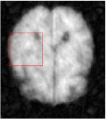
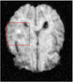
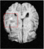
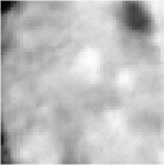
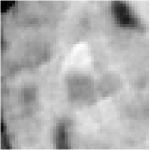
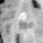
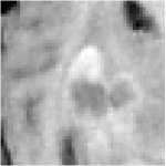
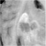
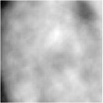
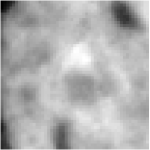
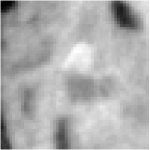
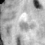
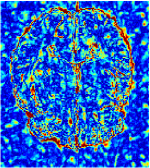
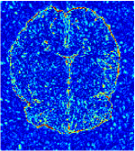
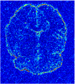
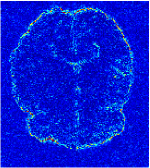
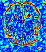
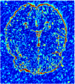
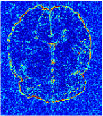
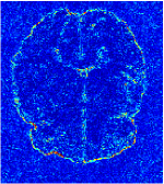
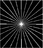
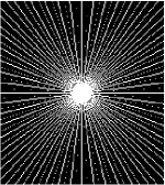
Figure 1: The pictures (from top to bottom) display the reconstruction results, zoomed in details, pointwise errors with colorbar and associated radio masks for meta-learning and conventional learning with four different CS ratios 10%, 20%, 30%, 40%éfrom left to right). The most top right one is ground truth fully-sampled image.

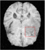
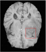
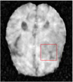
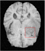
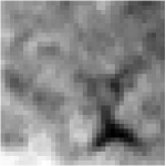
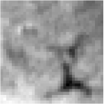
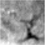
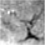
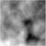
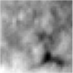
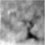
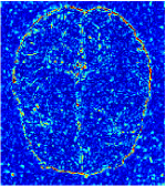
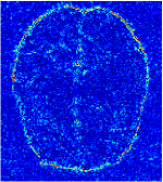
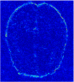
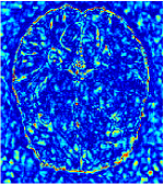
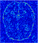
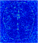
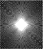
Figure 2: The pictures (from top to bottom) display the T1 Brain image reconstruction results, zoomed in details, pointwise errors with colorbar and associated radio masks for meta-learning and conventional learning. Meta-learning was trained with CS ratios 10%, 20%, 30% 40% and test with three different CS ratios 15%, 25% and 35%éfrom left to right). Conventional learning was trained and test with same CS ratios 15%, 25% and 35%. The most top right one is ground truth fully-sampled image.

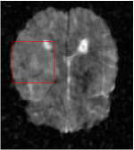
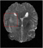
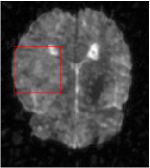
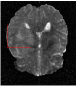
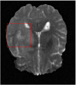
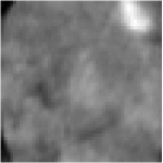
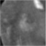
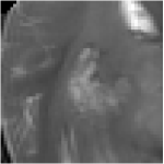
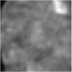
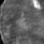
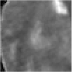
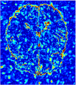
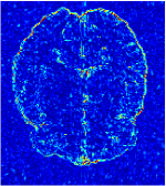
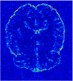
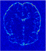
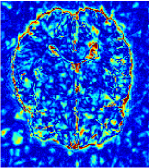
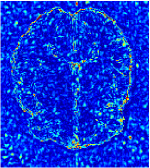
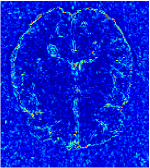
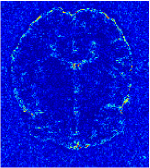
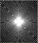
Figure 3: The pictures (from top to bottom) display the T2 Brain image reconstruction results, zoomed in details, pointwise errors with colorbar and associated radio masks for both these two compared methods with four different CS ratios 10%, 20%, 30%, 40%éfrom left to right). The most top right one is ground truth fully-sampled image.

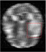
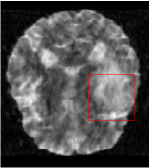
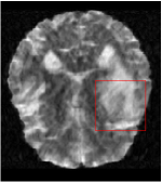
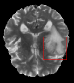
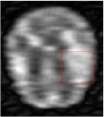
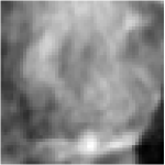
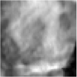
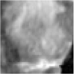
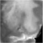
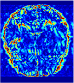
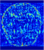
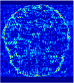
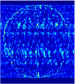
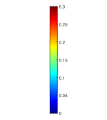
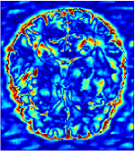
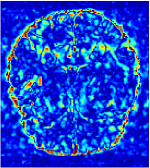
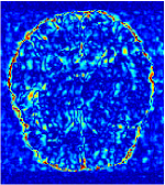
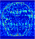
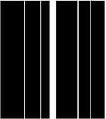
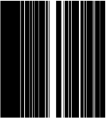
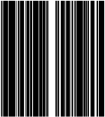
Figure 5: The pictures (from top to bottom) display the T2 Brain image reconstruction results, zoomed in details, pointwise errors with colorbar and associated Cartesian masks for both these two compared methods with four different CS ratios 10%, 20%, 30%, 40%éfrom left to right). The most top right one is ground truth fully-sampled image.

All the experiments are implemented on a Windows workstation with Intel Core i9 CPU at 3.3GHz and an Nvidia GTX-1080Ti GPU with 11GB of graphics card memory via TensorFlow Abadi et al. (2016). The parameters in the proposed network are initialized by using Xavier initialization Glorot and Bengio (2010). We trained the meta-learning network with four tasks synergistically associated with four different CS ratios: 10%, 20%, 30%, and 40%, and test the well-trained model on the testing dataset with the same masks of these four ratios. We have 300 training data for each CS ratio, which amount to total of 1200 images in the training dataset. The results for $T1$ and $T2$ MR reconstructions are shown in Tables 5.4 and 5.4 respectively. The associated reconstructed images are displayed in Figures 1 and 3. We also test the well-trained meta-learning model on unseen tasks with radio masks for skewed ratios: 15%, 25%, 35%, and random Cartesian masks with ratios 10%, 20%, 30% and 40%. The task-specific parameter for the unseen tasks are retrained for different masks with different sampling ratios individually with fixed task-invariant parameters $\theta$. In this experiments, we only need to learn $\omega_{i}$ for three skewed CS ratios with radio mask and four regular CS ratios with Cartesian masks. The experimental training proceed on less data and iterations, where we performed on 100 MR images with 50 epochs. For example, for reconstructing MR images with CS ratio 15% radio mask, we fix the parameter $\theta$ and retrain the task-specific parameter $\omega$ on 100 raw data with 50 epochs, then test with renewed $\omega$ on our testing data set with raw measurement that sampled from radio mask with CS ratio 15%. The results associated with radio masks are shown in Table 5.4 and 5.4, Figure 2 and 4 for $T1$ and $T2$ images respectively. The results associated with Cartesian masks are list in Table 5.4 and reconstructed images are displayed in Figure 5.

We compared proposed meta-learning method with conventional supervised learning, which was trained with one task at each time, and only learns task-invariant parameter $\theta$ without task-specific parameter $\omega_{i}$. The forward network of conventional learning unrolls Algorithm 1 with 11 phases which is the same as meta-learning. We merged training set and validation set which result in $450$ images for training the conventional supervised learning. The training batch size was set as 25 and applied total of 2000 epochs, while in meta-learning we applied 100 epochs with batch size 8. Same testing set was used in both meta-learning and conventional learning to evaluate the performance these two methods.

We made comparisons between meta-learning and the conventional network on these seven different CS ratios (10%, 20%, 30%, 40%, 15%, 25%, and 35%) in terms of two types of random under-sampling patterns: radio mask and Cartesian mask. The parameters for both meta-learning and conventional learning networks are trained via Adam optimizer Kingma and Ba (2015), and they both learn the forward unrolled task-invariant parameter $\theta$. Network training of conventional method uses the same network configuration as meta-learning network in terms of the number of convolutions, depth and size of CNN kernels, phase numbers and parameter initializer, etc. The major difference in the training process between these two methods is that meta-learning is proceed on multi-tasks by leveraging task-specific parameter $\omega_{i}$ that learned from Algorithm 2 and the common feature among tasks are learned from the feed forward network that unrolls Algorithm 1, while conventional learning solve for task specific problem by simply unrolls forward network via Algorithm 1 where both training and testing are implemented on the same task. To investigate the generalizability of meta-learning, we test the well-trained meta-learning model on MR images in different distributions in terms of two types of sampling masks with various trajectories. Training and testing of conventional learning are applied with the same CS ratios, that is, if the conventional method trained on CS ratio 10% then will be tested on a dataset with CS ratio 10%, etc.

Because of the nature of MR images are represented as complex-value, we applied complex convolutions Wang et al. (2020) for each CNN, that is, every kernel consists real part and imaginary part. Total of 11 phases are achieved if we set the termination condition $\epsilon_{\mathrm{tol}}=1\times 10^{-5}$ and the parameters of each phase are shared except for the step sizes. Three convolutions are used in $\mathbf{g}$, each convolution contains 4 filters with spatial kernel size $3\times 3$. We set $\nu_{\delta}=0.95$ and the parameter $\delta$ in Algorithm 2 was initialized as $\delta_{0}=1\times 10^{-3}$ stopped at value $\delta_{tol}=4.35\times 10^{-6}$, and we set total of 100 epochs. For training conventional method we set 2000 epochs with same number of phase, convolutions and kernel sizes as meta-learning. Initial $\lambda$ was set as $1\times 10^{-5}$ and $\nu_{\lambda}=1.001$.

We evaluate our reconstruction results on testing data sets using three metrics: PSNR, structural similarity (SSIM) Wang et al. (2004) and normalized mean squared error NMSE. The following formulations compute the PSNR, SSIM and NMSE between reconstructed image $\mathbf{x}$ and ground truth $\hat{\mathbf{x}}$.

$$PSNR=20\log_{10}\big{(}\max(\lvert\hat{\mathbf{x}}\rvert)\big{/}\frac{1}{N}\|\hat{\mathbf{x}}-\mathbf{x}\|^{2}\big{)},$$ (20)

where $N$ is the total number of pixels of ground truth.

$$SSIM=\frac{(2\mu_{\mathbf{x}}\mu_{\hat{\mathbf{x}}}+C_{1})(2\sigma_{\mathbf{x}\hat{\mathbf{x}}}+C_{2})}{(\mu_{\mathbf{x}}^{2}+\mu_{\hat{\mathbf{x}}}^{2}+C_{1})(\sigma_{\mathbf{x}}^{2}+\sigma_{\hat{\mathbf{x}}}^{2}+C_{2})},$$ (21)

where $\mu_{\mathbf{x}},\mu_{\hat{\mathbf{x}}}$ represent local means, $\sigma_{\mathbf{x}},\sigma_{\hat{\mathbf{x}}}$ denote standard deviations and $\sigma_{\mathbf{x}\hat{\mathbf{x}}}$ covariance between $\mathbf{x}$ and $\hat{\mathbf{x}}$, $C_{1}=(k_{1}L)^{2},C_{2}=(k_{2}L)^{2}$ are two constants which avoid zero denominator, and $k_{1}=0.01,k_{2}=0.03$. $L$ is the largest pixel value of MR image.

$$NMSE(\mathbf{x},\hat{\mathbf{x}})=\frac{\|\mathbf{x}-\hat{\mathbf{x}}\|_{2}^{2}}{\|\mathbf{x}\|_{2}^{2}}.$$ (22)

5.3 Quantitative and Qualitative Comparisons at different trajectories in radio mask

We evaluate the performance of well-trained Meta-learning and conventional learning. Table 5.4, 5.4 and 5.4 report the quantitative results of averaged numerical performance with standard deviations and associated descaled task specific meta-knowledge $\sigma(\omega_{i})$. From the experiments that implemented with radio masks, we observe that the average PSNR value of Meta-learning has improved 1.54 dB in T1 brain image among all the four CS ratios comparing to conventional method, and for T2 brain image, Meta-learning improved 1.46 dB in PSNR. Since the general setting of Meta-learning aims to take advantage of the information provided from each individual task, each task associate with an individual sampling mask that may have complemented sampled points, the performance of the reconstruction from each task benefits from other tasks. Smaller CS ratios will inhibit the reconstruction accuracy, due to the sparse undersampled trajectory in raw measurement, while Meta-learning exhibits the favorable potential ability to solve this issue even in the situation of insufficient amount of training data.

In general supervised learning, training data need to be in the same or similar distribution, heterogeneous data exhibits different structure variations of features which hinders CNNs to extract features efficiently. In our experiments, raw measurements sampled from different ratios of compressed sensing display different levels of incompleteness, these undersampled measurements do not fall in the same distribution but they are related. Different sampling masks are shown at the bottom of Figure 1 and 2 may have complemented sampled points, in the sense that some of the points which $40\%$ sampling ratio mask does not sample have been captured by other masks. In our experiment, different sampling masks provide their own information from their sampled points so that four reconstruction tasks help each other to achieve an efficient performance. Therefore, it explains the reason that Meta-learning is still superior to conventional learning when the sampling ratio is large.

Meta-learning expands a new paradigm for supervised learning, the purpose is to quickly learn multiple tasks. Meta-learning only needs to learn task-invariant parameters one time for the common feature that can be shared with four different tasks, and each $\sigma(\omega_{i})$ provides the task-specific weighting parameters which give the guidance as "learning to learn". Comparing to conventional learning, which needs to be trained four times with four different masks since the task-invariant parameter cannot be generalized to other tasks, which is time-intensive. From Table 5.4 and 5.4, we observe that small CS ratio needs higher value of $\sigma(\omega_{i})$. In fact, in our model (3) the task-specific parameters behave as weighted constraints for task-specific regularizers, and the tables indicate that lower CS ratios require larger weights to apply on the regularization.

Qualitative comparison between conventional and Meta-learning methods are shown in Figure 1 and 3, which display the reconstructed MR images of the same slice for T1 and T2 respectively, we label the zoomed-in details of HGG in the red boxes. We observe the evidence that conventional learning is more blurry and lost sharp edges, especially in lower CS ratios. From the point-wise error map, we find meta-learning has the ability to reduce noises especially in some detailed and complicated regions comparing to conventional learning.

5.4 Quantitative and Qualitative Comparisons at skewed trajectories in different sampling patterns

In this section, we test the generalizability of the proposed model that tests on unseen tasks. We fix the well-trained task-invariant parameter $\theta$ and only train $\omega_{i}$ for sampling ratios 15%, 25% and 35% with radio masks and sampling ratios 10%, 20%, 30% and 40% with Cartesian masks. In this experiment, we only used 100 training data for each CS ratio and apply a total of 50 epochs. The averaged evaluation values and standard deviations are listed in Table 5.4 and 5.4 for reconstructed T1 and T2 brain images respectively that proceed with radio masks, and Table 5.4 shows the qualitative performance for reconstructed T2 brain image that applied random Cartesian sampling masks. In T1 image reconstruction results, meta-learning improved 1.6921 dB in PSNR for 15% CS ratio, 1.6608 dB for 25% CS ratio, and 0.5764 dB for 35% comparing to the conventional method, which in the tendency that the level of reconstruction quality for lower CS ratios improved more than higher CS ratios. A similar trend happens in T2 reconstruction results with different sampling masks. The qualitative comparisons are illustrated in Figure 2, 4 and 5 for T1 and T2 images tested in skewed CS ratios in radio masks, and T2 images tested in Cartesian masks with regular CS ratios respectively. In the experiments that conducted with radio masks, meta-learning is superior to conventional learning especially at CS ratio 15%, one can observe that the detailed region in red boxes keeps edges and is more close to the true image, while conventional method reconstructions are hazier and lost details in some complicated tissue. The point-wise error map also indicates that Meta-learning has the ability to suppress noises.

Training with Cartesian masks is more difficult than radio masks, especially for conventional learning where the network is not very deep since the network only applied three convolutions each with four kernels. Table 5.4 indicates that the average performance of meta-learning improved about 1.87 dB comparing to conventional methods with T2 brain images. These results further demonstrate that meta-learning has the benefit of parameter efficiency, the performance is much better than conventional learning even if we apply a shallow network with small size of training data.

The numeric experimental results discussed above intimates that Meta-learning is capable of fast adaption to new tasks and has more robust generalizability for a broad range of tasks with heterogeneous diverse data. Meta-learning can be considered as an efficient technique for solving difficult tasks by leveraging the features extracted from easier tasks.

[htb] Quantitative evaluations of the reconstructions on T1 brain image associated with various sampling ratios of radial masks. CS Ratio Methods PSNR SSIM NMSE $\sigma(\omega_{i})$ 10% Conventional 21.7570 $\pm$ 1.0677 0.5550 $\pm$ 0.0412 0.0259 $\pm$ 0.0082 Meta-learning 23.2672 $\pm$ 1.1229 0.6101 $\pm$ 0.0436 0.0184 $\pm$ 0.0067 0.9218 20% Conventional 26.6202 $\pm$ 1.1662 0.6821 $\pm$ 0.0397 0.0910 $\pm$ 0.0169 Meta-learning 28.2944 $\pm$ 1.2119 0.7640 $\pm$ 0.0377 0.0058 $\pm$ 0.0022 0.7756 30% Conventional 29.5034 $\pm$ 1.4446 0.7557 $\pm$ 0.0408 0.0657 $\pm$ 0.0143 Meta-learning 31.1417 $\pm$ 1.5866 0.8363 $\pm$ 0.0385 0.0031 $\pm$ 0.0014 0.6501 40% Conventional 31.4672 $\pm$ 1.6390 0.8111 $\pm$ 0.0422 0.0029 $\pm$ 0.0014 Meta-learning 32.8238 $\pm$ 1.7039 0.8659 $\pm$ 0.0370 0.0022 $\pm$ 0.0010 0.6447

[htb] Quantitative evaluations of the reconstructions on T1 brain image associated with various sampling ratios of radial masks. Meta-learning was trained with CS ratio 10%, 20%, 30% and 40% and test with skewed ratios 15%, 25% and 35%. Conventional method performed regular training and testing on same CS ratios 15%, 25% and 35%. CS Ratio Metods PSNR SSIM NMSE $\sigma(\omega_{i})$ 15% Conventional 24.6573 $\pm$ 1.0244 0.6339 $\pm$ 0.0382 0.1136 $\pm$ 0.0186 Meta-learning 26.3494 $\pm$ 1.0102 0.7088 $\pm$ 0.0352 0.0090 $\pm$ 0.0030 0.9429 25% Conventional 28.4156 $\pm$ 1.2361 0.7533 $\pm$ 0.0368 0.0741 $\pm$ 0.0141 Meta-learning 30.0764 $\pm$ 1.4645 0.8135 $\pm$ 0.0380 0.0040 $\pm$ 0.0017 0.8482 35% Conventional 31.5320 $\pm$ 1.5242 0.7923 $\pm$ 0.0420 0.0521 $\pm$ 0.0119 Meta-learning 32.1084 $\pm$ 1.6481 0.8553 $\pm$ 0.0379 0.0025 $\pm$ 0.0011 0.6552

[H] Quantitative evaluations of the reconstructions on T2 brain image associated with various sampling ratios of radial masks. CS Ratio Metods PSNR SSIM NMSE $\sigma(\omega_{i})$ 10% Conventional 23.0706 $\pm$ 1.2469 0.5963 $\pm$ 0.0349 0.2158 $\pm$ 0.0347 Meta-learning 24.0842 $\pm$ 1.3863 0.6187 $\pm$ 0.0380 0.0112 $\pm$ 0.0117 0.9013 20% Conventional 27.0437 $\pm$ 1.0613 0.6867 $\pm$ 0.0261 0.1364 $\pm$ 0.0213 Meta-learning 28.9118 $\pm$ 1.0717 0.7843 $\pm$ 0.0240 0.0122 $\pm$ 0.0030 0.8742 30% Conventional 29.5533 $\pm$ 1.0927 0.7565 $\pm$ 0.0265 0.1023 $\pm$ 0.0166 Meta-learning 31.4096 $\pm$ 0.9814 0.8488 $\pm$ 0.0217 0.0069 $\pm$ 0.0019 0.8029 40% Conventional 32.0153 $\pm$ 0.9402 0.8139 $\pm$ 0.0238 0.0770 $\pm$ 0.0128 Meta-learning 33.1114 $\pm$ 1.0189 0.8802 $\pm$ 0.0210 0.0047 $\pm$ 0.0015 0.7151

[H] Quantitative evaluations of the reconstructions on T2 brain image associated with various sampling ratios of radial masks. Meta-learning was trained with CS ratio 10%, 20%, 30% and 40% and test with 15%, 25% and 35%. Conventional method performed regular training and testing on same CS ratios 15%, 25% and 35%. CS Ratio Metods PSNR SSIM NMSE $\sigma(\omega_{i})$ 15% Conventional 24.8921 $\pm$ 1.2356 0.6259 $\pm$ 0.0285 0.1749 $\pm$ 0.0280 Meta-learning 26.7031 $\pm$ 1.2553 0.7104 $\pm$ 0.0318 0.0205 $\pm$ 0.0052 0.9532 25% Conventional 29.0545 $\pm$ 1.1980 0.7945 $\pm$ 0.0292 0.1083 $\pm$ 0.0173 Meta-learning 30.0698 $\pm$ 0.9969 0.8164 $\pm$ 0.0235 0.0093 $\pm$ 0.0022 0.8595 35% Conventional 31.5201 $\pm$ 1.0021 0.7978 $\pm$ 0.0236 0.0815 $\pm$ 0.0129 Meta-learning 32.0683 $\pm$ 0.9204 0.8615 $\pm$ 0.0209 0.0059 $\pm$ 0.0014 0.7388

[H] Quantitative evaluations of the reconstructions on T2 brain image associated with various sampling ratios of random Cartesian masks. CS Ratio Metods PSNR SSIM NMSE $\sigma(\omega_{i})$ 10% Conventional 20.8867 $\pm$ 1.2999 0.5082 $\pm$ 0.0475 0.0796 $\pm$ 0.0242 Meta-learning 22.0434 $\pm$ 1.3555 0.6279 $\pm$ 0.0444 0.0611 $\pm$ 0.0188 0.9361 20% Conventional 22.7954 $\pm$ 1.2819 0.6057 $\pm$ 0.0412 0.0513 $\pm$ 0.0157 Meta-learning 24.7162 $\pm$ 1.3919 0.6971 $\pm$ 0.0380 0.0329 $\pm$ 0.0101 0.8320 30% Conventional 24.2170 $\pm$ 1.2396 0.6537 $\pm$ 0.0360 0.0371 $\pm$ 0.0117 Meta-learning 26.4537 $\pm$ 1.3471 0.7353 $\pm$ 0.0340 0.0221 $\pm$ 0.0068 0.6771 40% Conventional 25.3668 $\pm$ 1.3279 0.6991 $\pm$ 0.0288 0.1657 $\pm$ 0.0265 Meta-learning 27.5367 $\pm$ 1.4107 0.7726 $\pm$ 0.0297 0.0171 $\pm$ 0.0050 0.6498

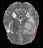
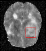
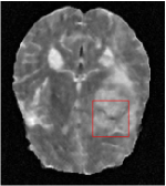
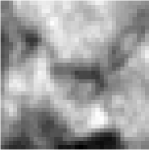
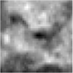
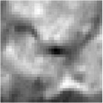
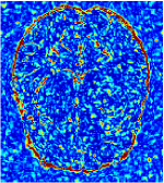
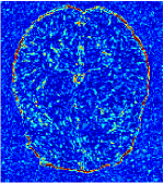
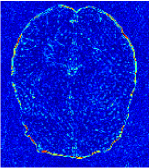
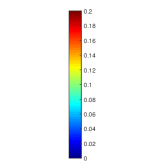
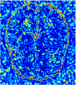
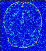
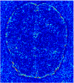
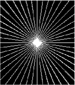
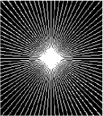
Figure 4: The pictures (from top to bottom) display the T2 Brain image reconstruction results, zoomed in details, pointwise errors with colorbar and associated radio masks for meta-learning and conventional learning. Meta-learning was trained with CS ratios 10%, 20%, 30% 40% and test with three different CS ratios 15%, 25% and 35%éfrom left to right). Conventional learning was trained and test with same CS ratios 15%, 25% and 35%. The most top right one is ground truth fully-sampled image.

5.5 Future work and open challenges

Deep optimization-based meta-learning techniques have shown great generalizability but there are several open challenges that can be discussed and can potentially be addressed in future work. A major issue is the memorization problem since the base learner needs to be optimized for a large number of phases and the training algorithm contains multiple gradient steps, computation cost is very expensive in terms of time and memory costs. In addition to reconstruct MRI through different trajectories, another potential application for medical imaging could be multi-modality reconstruction and synthesis. Capturing images of anatomy with multi-modality acquisitions enhances the diagnostic information, and could be cast as a multi-task problem and benefit from meta-learning.

6 Conclusions

In this paper, we put forward a novel deep model for MRI reconstructions via meta-learning. The proposed method has the ability to solve multi-tasks synergistically and the well-trained model could generalize well to new tasks. Our baseline network is constructed by unfolds an LOA, which inherits convergence property, improves the interpretability, and promotes parameter efficiency of the designed network structure. The designated adaptive regularizer consists task-invariant learner and a task-specific meta-knowledge. Network training follows a bilevel optimization algorithm that minimizes task-specific parameter $\omega$ in the upper level on validation data and minimizes task-invariant parameters $\theta$ on training data with fixed $\omega$. The proposed approach is the first model for solving the inverse problem by applying meta-training on the adaptive regularization in the variational model. We consider recovering undersampled raw data across different sampling trajectories with various sampling patterns as different tasks. Extensive numerical experiments on various MRI datasets demonstrate that the proposed method generalizes well at various sampling trajectories and is capable of fast adaption to the unseen trajectories and sampling patterns. The reconstructed images achieve higher quality comparing to conventional supervised learning for both seen and unseen k-space trajectory cases.

yes

Appendix A Convergence Analysis

We make the following assumptions on $f$ and $\mathbf{g}$ throughout this work:

• (a1): $f$ is differentiable and (possibly) nonconvex, and $\nabla f$ is $L_{f}$-Lipschitz continuous.

• (a2): Every component of $\mathbf{g}$ is differentiable and (possibly) nonconvex, $\nabla\mathbf{g}$ is $L_{g}$-Lipschitz continuous.

• (a3): $\sup_{\mathbf{x}\in\mathcal{X}}\|\nabla\mathbf{g}(\mathbf{x})\|\leq M$ for some constant $M>0$.

• (a4): $\phi$ is coercive, and $\phi^{*}=\min_{\mathbf{x}\in\mathcal{X}}\phi(\mathbf{x})>-\infty$.

First we state the Clark Subdifferential Chen et al. (2020) of $r(\mathbf{x})$ in Lemma A and we provide that the gradient of $r_{\varepsilon}$ is Lipschitz continuous in Lemma A.

Lemma .

Let $r(\mathbf{x})$ be defined in (4), then the Clarke subdifferential of $r$ at $\mathbf{x}$ is

$$\partial r(\mathbf{x})=\{\sum_{j\in I_{0}}\nabla\mathbf{g}_{i}(\mathbf{x})^{\top}\mathbf{w}_{j}+\sum_{j\in I_{1}}\nabla\mathbf{g}_{j}(\mathbf{x})^{\top}\frac{\mathbf{g}_{j}(\mathbf{x})}{\|\mathbf{g}_{j}(\mathbf{x})\|}\ \bigg{|}\ \mathbf{w}_{j}\in\mathbb{R}^{d},\ \|\Pi(\mathbf{w}_{j};\mathcal{C}(\nabla\mathbf{g}_{i}(\mathbf{x})))\|\leq 1,\ \forall\,j\in I_{0}\},$$ (23)

where $I_{0}=\{j\in[m]\ |\ \|\mathbf{g}_{j}(\mathbf{x})\|=0\}$, $I_{1}=[m]\setminus I_{0}$, and $\Pi(\mathbf{w};\mathcal{C}(\mathbf{A}))$ is the projection of $\mathbf{w}$ onto $\mathcal{C}(\mathbf{A})$ which stands for the column space of $\mathbf{A}$.

Lemma .

The gradient of $r_{\varepsilon}$ is Lipschitz continuous with constant $m(L_{g}+\frac{2M^{2}}{\varepsilon})$.

Proof.

From $r_{\varepsilon}(\mathbf{x})=\sum^{m}_{j=1}(\|\mathbf{g}_{j}(\mathbf{x})\|^{2}+\varepsilon^{2})^{\frac{1}{2}}-\varepsilon$, it follows that

$$\nabla r_{\varepsilon}(\mathbf{x})=\sum^{m}_{j=1}\nabla\mathbf{g}_{j}(\mathbf{x})^{\top}\mathbf{g}_{j}(\mathbf{x})(\|\mathbf{g}_{j}(\mathbf{x})\|^{2}+\varepsilon^{2})^{-\frac{1}{2}}.$$ (24)

For any $\mathbf{x}_{1},\mathbf{x}_{2}\in\mathcal{X}$, we first define $h(\mathbf{x})=\mathbf{g}_{j}(\mathbf{x})(\|\mathbf{g}_{j}(\mathbf{x})\|^{2}+\varepsilon^{2})^{-\frac{1}{2}}$, so $\lVert h(\mathbf{x})\rVert<1$.

$$\left\|h(\mathbf{x}_{1})-h(\mathbf{x}_{2})\right\|$$ (25a)

$$=\left\|\frac{\mathbf{g}_{j}(\mathbf{x}_{1})}{\sqrt{\|\mathbf{g}_{j}(\mathbf{x}_{1})\|^{2}+\varepsilon^{2}}}-\frac{\mathbf{g}_{j}(\mathbf{x}_{2})}{\sqrt{\|\mathbf{g}_{j}(\mathbf{x}_{2})\|^{2}+\varepsilon^{2}}}\right\|$$ (25b)

$$=\left\|\frac{\mathbf{g}_{j}(\mathbf{x}_{1})}{\sqrt{\|\mathbf{g}_{j}(\mathbf{x}_{1})\|^{2}+\varepsilon^{2}}}-\frac{\mathbf{g}_{j}(\mathbf{x}_{1})}{\sqrt{\|\mathbf{g}_{j}(\mathbf{x}_{2})\|^{2}+\varepsilon^{2}}}+\frac{\mathbf{g}_{j}(\mathbf{x}_{1})}{\sqrt{\|\mathbf{g}_{j}(\mathbf{x}_{2})\|^{2}+\varepsilon^{2}}}-\frac{\mathbf{g}_{j}(\mathbf{x}_{2})}{\sqrt{\|\mathbf{g}_{j}(\mathbf{x}_{2})\|^{2}+\varepsilon^{2}}}\right\|$$ (25c)

$$\leq\left\|\mathbf{g}_{j}(\mathbf{x}_{1})\left(\frac{\sqrt{\|\mathbf{g}_{j}(\mathbf{x}_{2})\|^{2}+\varepsilon^{2}}-\sqrt{\|\mathbf{g}_{j}(\mathbf{x}_{1})\|^{2}+\varepsilon^{2}}}{\sqrt{\|\mathbf{g}_{j}(\mathbf{x}_{1})\|^{2}+\varepsilon^{2}}\sqrt{\|\mathbf{g}_{j}(\mathbf{x}_{2})\|^{2}+\varepsilon^{2}}}\right)\right\|+\left\|\frac{\mathbf{g}_{j}(\mathbf{x}_{1})-\mathbf{g}_{j}(\mathbf{x}_{2})}{\sqrt{\|\mathbf{g}_{j}(\mathbf{x}_{2})\|^{2}+\varepsilon^{2}}}\right\|$$ (25d)

$$\leq\left\|\frac{\mathbf{g}_{j}(\mathbf{x}_{1})}{\sqrt{\|\mathbf{g}_{j}(\mathbf{x}_{1})\|^{2}+\varepsilon^{2}}}\right\|\left\|\frac{\sqrt{\|\mathbf{g}_{j}(\mathbf{x}_{2})\|^{2}+\varepsilon^{2}}-\sqrt{\|\mathbf{g}_{j}(\mathbf{x}_{1})\|^{2}+\varepsilon^{2}}}{\sqrt{\|\mathbf{g}_{j}(\mathbf{x}_{2})\|^{2}+\varepsilon^{2}}}\right\|+\frac{1}{\varepsilon}\left\|\mathbf{g}_{j}(\mathbf{x}_{1})-\mathbf{g}_{j}(\mathbf{x}_{2})\right\|$$ (25e)

$$\leq\frac{1}{\varepsilon}\left\|\sqrt{\|\mathbf{g}_{j}(\mathbf{x}_{2})\|^{2}+\varepsilon^{2}}-\sqrt{\|\mathbf{g}_{j}(\mathbf{x}_{1})\|^{2}+\varepsilon^{2}}\right\|+\frac{1}{\varepsilon}\left\|\mathbf{g}_{j}(\mathbf{x}_{1})-\mathbf{g}_{j}(\mathbf{x}_{2})\right\|$$ (25f)

$$\leq\frac{1}{\varepsilon}\frac{\|\mathbf{g}_{j}(\mathbf{x}_{2})\|^{2}-\|\mathbf{g}_{j}(\mathbf{x}_{1})\|^{2}}{\sqrt{\|\mathbf{g}_{j}(\mathbf{x}_{2})\|^{2}+\varepsilon^{2}}+\sqrt{\|\mathbf{g}_{j}(\mathbf{x}_{1})\|^{2}+\varepsilon^{2}}}+\frac{1}{\varepsilon}\left\|\mathbf{g}_{j}(\mathbf{x}_{1})-\mathbf{g}_{j}(\mathbf{x}_{2})\right\|$$ (25g)

$$\leq\frac{1}{\varepsilon}\underbrace{\frac{\|\mathbf{g}_{j}(\mathbf{x}_{2})\|+\|\mathbf{g}_{j}(\mathbf{x}_{1})\|}{\sqrt{\|\mathbf{g}_{j}(\mathbf{x}_{2})\|^{2}+\varepsilon^{2}}+\sqrt{\|\mathbf{g}_{j}(\mathbf{x}_{1})\|^{2}+\varepsilon^{2}}}}_{<1}\left(\|\mathbf{g}_{j}(\mathbf{x}_{2})\|-\|\mathbf{g}_{j}(\mathbf{x}_{1})\|\right)+\frac{1}{\varepsilon}\left\|\mathbf{g}_{j}(\mathbf{x}_{1})-\mathbf{g}_{j}(\mathbf{x}_{2})\right\|$$ (25h)

$$\leq\frac{1}{\varepsilon}\left\|\mathbf{g}_{j}(\mathbf{x}_{2})-\mathbf{g}_{j}(\mathbf{x}_{1})\right\|+\frac{1}{\varepsilon}\left\|\mathbf{g}_{j}(\mathbf{x}_{1})-\mathbf{g}_{j}(\mathbf{x}_{2})\right\|$$ (25i)

$$=\frac{2}{\varepsilon}\left\|\mathbf{g}_{j}(\mathbf{x}_{1})-\mathbf{g}_{j}(\mathbf{x}_{2})\right\|.$$ (25j)

where to get (25f) we used $\left\|\frac{\mathbf{g}_{j}(\mathbf{x}_{1})}{\sqrt{\|\mathbf{g}_{j}(\mathbf{x}_{1})\|^{2}+\varepsilon^{2}}}\right\|<1\text{ and }\frac{1}{\sqrt{\|\mathbf{g}_{j}(\mathbf{x}_{1})\|^{2}+\varepsilon^{2}}}<\frac{1}{\varepsilon}$.

Therefore we have:

$$\left\|\nabla r_{\varepsilon}(\mathbf{x}_{1})-\nabla r_{\varepsilon}(\mathbf{x}_{2})\right\|$$ (26a)

$$=\sum^{m}_{j=1}\left\|\nabla\mathbf{g}_{j}(\mathbf{x}_{1})^{\top}h(\mathbf{x}_{1})-\nabla\mathbf{g}_{j}(\mathbf{x}_{2})^{\top}h(\mathbf{x}_{2})\right\|$$ (26b)

$$=\sum^{m}_{j=1}\left\|\nabla\mathbf{g}_{j}(\mathbf{x}_{1})^{\top}h(\mathbf{x}_{1})-\nabla\mathbf{g}_{j}(\mathbf{x}_{2})^{\top}h(\mathbf{x}_{1})+\nabla\mathbf{g}_{j}(\mathbf{x}_{2})^{\top}h(\mathbf{x}_{1})-\nabla\mathbf{g}_{j}(\mathbf{x}_{2})^{\top}h(\mathbf{x}_{2})\right\|$$ (26c)

$$\leq\sum^{m}_{j=1}\left\|\left(\nabla\mathbf{g}_{j}(\mathbf{x}_{1})-\nabla\mathbf{g}_{j}(\mathbf{x}_{2})\right)^{\top}h(\mathbf{x}_{1})\right\|+\left\|\nabla\mathbf{g}_{j}(\mathbf{x}_{2})\left(h(\mathbf{x}_{1})-h(\mathbf{x}_{2})\right)\right\|$$ (26d)

$$\leq\sum^{m}_{j=1}\left\|\nabla\mathbf{g}_{j}(\mathbf{x}_{1})-\nabla\mathbf{g}_{j}(\mathbf{x}_{2})\right\|\lVert h(\mathbf{x}_{1})\rVert+\lVert\nabla\mathbf{g}_{j}(\mathbf{x}_{2})\rVert\left\|h(\mathbf{x}_{1})-h(\mathbf{x}_{2})\right\|$$

$$\leq\sum^{m}_{j=1}\left\|\nabla\mathbf{g}_{j}(\mathbf{x}_{1})-\nabla\mathbf{g}_{j}(\mathbf{x}_{2})\right\|+\lVert\nabla\mathbf{g}_{j}(\mathbf{x}_{2})\rVert\frac{2}{\varepsilon}\lVert\mathbf{g}_{j}(\mathbf{x}_{1})-\mathbf{g}_{j}(\mathbf{x}_{2})\rVert\text{ by }\eqref{eq:h1-h2}\text{ and }$$ (26e)

$$\leq m(L_{g}\lVert\mathbf{x}_{1}-\mathbf{x}_{2}\rVert+M\frac{2}{\varepsilon}\cdot M\lVert\mathbf{x}_{1}-\mathbf{x}_{2}\rVert),$$ (26f)

where the first term of the last inequality is due to the $L_{g}$-Lipschitz continuity of $\nabla\mathbf{g}_{j}$. The second term is because of $\lVert\mathbf{g}_{j}(\mathbf{x}_{1})-\mathbf{g}_{j}(\mathbf{x}_{2})\rVert=\lVert\nabla\mathbf{g}_{j}(\tilde{\mathbf{x}})(\mathbf{x}_{1}-\mathbf{x}_{2})\rVert$ for some $\tilde{\mathbf{x}}\in\mathcal{X}$ due to the mean value theorem and $\|\nabla\mathbf{g}_{j}(\tilde{\mathbf{x}})\|\leq\sup_{\mathbf{x}\in\mathcal{X}}\|\nabla\mathbf{g}_{j}(\mathbf{x})\|\leq M$. Therefore we get

$$\left\|\nabla r_{\varepsilon}(\mathbf{x}_{1})-\nabla r_{\varepsilon}(\mathbf{x}_{2})\right\|\leq m(L_{g}+\frac{2M^{2}}{\varepsilon})\lVert\mathbf{x}_{1}-\mathbf{x}_{2}\rVert.$$ (27)

∎

Lemma .

Let $\varepsilon,\eta,\tau_{t},a>0$, $0<\rho<1$, choose initial $\mathbf{x}_{0}\in\mathcal{X}$. Suppose the sequence $\{\mathbf{x}_{t}\}$ is generated by executing Lines 3-14 of Algorithm 1 with fixed $\varepsilon_{t}=\varepsilon$ and exists $0<\delta<\frac{L_{\varepsilon}}{2/a+L_{\varepsilon}}<1$ such that $\alpha_{t}\geq\frac{\delta}{L_{\varepsilon}}>0$, where $L_{\varepsilon}=L_{f}+L_{h}+mL_{g}+\frac{2M^{2}}{\varepsilon}$ and $\phi^{*}:=\min_{\mathbf{x}\in\mathcal{X}}\phi(\mathbf{x})$. Then the following statements hold:

1. $\|\nabla\phi_{\varepsilon}(\mathbf{x}_{t})\|\to 0$ as $t\to\infty$.

2. $\max\{t\in\mathbb{N}\ |\ \lVert\nabla\phi_{\varepsilon}(\mathbf{x}_{t+1})\rVert\geq\eta\}\leq\max\{\frac{{aL^{2}_{\varepsilon}}}{\delta^{2}},a^{3}\}\left(\phi_{\varepsilon}(\mathbf{x}_{0})-\phi^{*}+\varepsilon\right)$.

Proof.

1. In each iteration, we compute $\mathbf{u}_{t+1}=\mathbf{z}_{t+1}-\tau_{t}\sigma(\omega_{i})\nabla r_{\varepsilon_{t}}(\mathbf{z}_{t+1})$.

   1. In the case the condition

      $$\|\nabla\phi_{\varepsilon}(\mathbf{x}_{t})\|\leq a\|\mathbf{u}_{t+1}-\mathbf{x}_{t}\|\ \ \ \mbox{and}\ \ \ \phi_{\varepsilon}(\mathbf{u}_{t+1})-\phi_{\varepsilon}(\mathbf{x}_{t})\leq-\frac{1}{a}\|\mathbf{u}_{t+1}-\mathbf{x}_{t}\|^{2}$$ (28)

      holds with $a>0$, we put $\mathbf{x}_{t+1}=\mathbf{u}_{t+1}$, and we have $\phi_{\varepsilon}(\mathbf{u}_{t+1})\leq\phi_{\varepsilon}(\mathbf{x}_{t})$.

   2. Otherwise, we compute $\mathbf{v}_{t+1}=\mathbf{x}_{t}-\alpha_{t}\nabla\phi_{\varepsilon}(\mathbf{x}_{t})$, where $\alpha_{t}$ is found through the line search until the criteria

      $$\phi_{\varepsilon}(\mathbf{v}_{t+1})-\phi_{\varepsilon}(\mathbf{x}_{t})\leq-\frac{1}{a}\|\mathbf{v}_{t+1}-\mathbf{x}_{t}\|^{2}$$ (29)

      holds and then put $\mathbf{x}_{t+1}=\mathbf{v}_{t+1}$. From Lemma A we know that the gradient $\nabla r_{\varepsilon}(\mathbf{x})$ is Lipschitz continuous with constant $m(L_{g}+\frac{2M^{2}}{\varepsilon})$. Also we assumed in (a1) $\nabla f$ is $L_{f}$-Lipschitz continuous. Hence, putting $L_{\varepsilon}=L_{f}+m(L_{g}+\frac{2M^{2}}{\varepsilon})$, we get that $\nabla\phi_{\varepsilon}$ is $L_{\varepsilon}$-Lipschitz continuous, which implies

      $$\phi_{\varepsilon}(\mathbf{v}_{t+1})\leq\phi_{\varepsilon}(\mathbf{x}_{t})+\langle\nabla\phi_{\varepsilon}(\mathbf{x}_{t}),\mathbf{v}_{t+1}-\mathbf{x}_{t}\rangle+\frac{L_{\varepsilon}}{2}\|\mathbf{v}_{t+1}-\mathbf{x}_{t}\|^{2}.$$ (30)

      Also, by the optimality condition of

      $$\mathbf{v}_{t+1}=\operatorname*{arg\,min}_{\mathbf{x}}\langle\nabla f(\mathbf{x}_{t}),\mathbf{x}-\mathbf{x}_{t}\rangle+\sigma(\omega_{i})\langle\nabla r_{\varepsilon}(\mathbf{x}_{t}),\mathbf{x}-\mathbf{x}_{t}\rangle+\frac{1}{2\alpha_{t}}\|\mathbf{x}-\mathbf{x}_{t}\|^{2},$$

      we have

      $$\langle\nabla\phi_{\varepsilon}(\mathbf{x}_{t}),\mathbf{v}_{t+1}-\mathbf{x}_{t}\rangle+\frac{1}{2\alpha_{t}}\lVert\mathbf{v}_{t+1}-\mathbf{x}_{t}\rVert^{2}\leq 0.$$ (31)

      Combine (30) and (31) and $\mathbf{v}_{t+1}=\mathbf{x}_{t}-\alpha_{t}\nabla\phi_{\varepsilon}(\mathbf{x}_{t})$ in line 8 of Algorithm 1 yields

      $$\phi_{\varepsilon}(\mathbf{v}_{t+1})-\phi_{\varepsilon}(\mathbf{x}_{t})\leq-\left(\frac{1}{2\alpha_{t}}-\frac{L_{\varepsilon}}{2}\right)\lVert\mathbf{v}_{t+1}-\mathbf{x}_{t}\rVert^{2}.$$ (32)

      Therefore, it is enough for $\alpha_{t}\leq\frac{1}{2/a+L_{\varepsilon}}$ so that the criteria (29) is satisfied. This process only take finitely many iterations since we can find a finite $t$ such that $\rho^{t}\alpha_{t}\leq\frac{1}{2/a+L_{\varepsilon}}$ and through the line search we can get $\phi_{\varepsilon}(\mathbf{v}_{t+1})\leq\phi_{\varepsilon}(\mathbf{x}_{t})$.

   Therefore in either case of 11.1. or 11.2. where we take $\mathbf{x}_{t+1}=\mathbf{u}_{t+1}$ or $\mathbf{v}_{t+1}$, we can get

   $$\phi_{\varepsilon}(\mathbf{x}_{t+1})\leq\phi_{\varepsilon}(\mathbf{x}_{t}),\text{ for all }t\geq 0.$$ (33)

   Now from case 11.1., (28) gives

   $$\lVert\nabla\phi_{\varepsilon}(\mathbf{x}_{t})\rVert^{2}\leq a^{2}\left\|\mathbf{u}_{t+1}-\mathbf{x}_{t}\right\|^{2}\leq a^{3}\left(\phi_{\varepsilon}(\mathbf{x}_{t})-\phi_{\varepsilon}(\mathbf{u}_{t+1})\right),$$ (34a)

   therefore if $$\mathbf{x}_{t+1}=\mathbf{u}_{t+1} \lVert\nabla\phi_{\varepsilon}(\mathbf{x}_{t})\rVert^{2}\leq a^{3}\left(\phi_{\varepsilon}(\mathbf{x}_{t})-\phi_{\varepsilon}(\mathbf{x}_{t+1})\right).$$ we get (34b)

   From case 11.2. and $\mathbf{v}_{t+1}=\mathbf{x}_{t}-\alpha_{t}\nabla\phi_{\varepsilon}(\mathbf{x}_{t})$ we have

   $$\phi_{\varepsilon}(\mathbf{v}_{t+1})-\phi_{\varepsilon}(\mathbf{x}_{t})\leq -\frac{1}{a}\lVert\mathbf{v}_{t+1}-\mathbf{x}_{t}\rVert^{2}=-\frac{1}{a}\alpha_{t}^{2}\lVert\nabla\phi_{\varepsilon}(\mathbf{x}_{t})\rVert^{2}$$ (35a)

   $$\Longrightarrow \lVert\nabla\phi_{\varepsilon}(\mathbf{x}_{t})\rVert^{2}\leq\frac{a}{\alpha_{t}^{2}}\big{(}\phi_{\varepsilon}(\mathbf{x}_{t})-\phi_{\varepsilon}(\mathbf{v}_{t+1})\big{)},$$ (35b)

   then if $$\mathbf{x}_{t+1}=\mathbf{v}_{t+1} \lVert\nabla\phi_{\varepsilon}(\mathbf{x}_{t})\rVert^{2}\leq\frac{a}{\alpha_{t}^{2}}\big{(}\phi_{\varepsilon}(\mathbf{x}_{t})-\phi_{\varepsilon}(\mathbf{x}_{t+1})\big{)}.$$, we have (35c)

   Since $\frac{\delta}{L_{\varepsilon}}\leq\alpha_{t}\leq\frac{1}{2/a+L_{\varepsilon}}$, we have

   $$\lVert\nabla\phi_{\varepsilon}(\mathbf{v}_{t+1})\rVert^{2}\leq\frac{{aL^{2}_{\varepsilon}}}{\delta^{2}}\big{(}\phi_{\varepsilon}(\mathbf{v}_{t+1})-\phi_{\varepsilon}(\mathbf{x}_{t+1})\big{)}.$$ (36)

   Combining (34b) and (36) and select $C=\max\{\frac{{aL^{2}_{\varepsilon}}}{\delta^{2}},a^{3}\}$, we get

   $$\lVert\nabla\phi_{\varepsilon}(\mathbf{x}_{t})\rVert^{2}\leq C\big{(}\phi_{\varepsilon}(\mathbf{x}_{t})-\phi_{\varepsilon}(\mathbf{x}_{t+1})\big{)}.$$ (37)

   Summing up (37) for $t=0,\cdots,T$, we have

   $$\sum^{T}_{t=0}\lVert\nabla\phi_{\varepsilon}(\mathbf{x}_{t})\rVert^{2}\leq C\big{(}\phi_{\varepsilon}(\mathbf{x}_{0})-\phi_{\varepsilon}(\mathbf{x}_{T+1})\big{)},$$ (38)

   combining with the fact $\phi_{\varepsilon}(\mathbf{x})\geq\phi(\mathbf{x})-\varepsilon\geq\phi^{*}-\varepsilon$ for every $\mathbf{x}\in\mathcal{X}$, we have

   $$\sum^{T}_{t=0}\lVert\nabla\phi_{\varepsilon}(\mathbf{x}_{t})\rVert^{2}\leq C\left(\phi_{\varepsilon}(\mathbf{x}_{0})-\phi^{*}+\varepsilon\right).$$ (39)

   The right hand side is a finite constant and hence by letting $t\to\infty$ we know that $\lVert\nabla\phi_{\varepsilon}(\mathbf{x}_{t})\rVert\to 0$, which proves the first statement.

2. Denote $\kappa:=\max\{t\in\mathbb{N}\ |\ \lVert\nabla\phi_{\varepsilon}(\mathbf{x}_{t+1})\rVert\geq\eta\}$, then we know that $\lVert\nabla\phi_{\varepsilon}(\mathbf{x}_{t+1})\rVert\geq\eta$ for all $t\leq\kappa-1$. Hence we have

   $$\kappa\eta^{2}\leq\sum^{\kappa-1}_{t=0}\lVert\nabla\phi_{\varepsilon}(\mathbf{x}_{t+1})\rVert^{2}=\sum^{\kappa}_{t=1}\lVert\nabla\phi_{\varepsilon}(\mathbf{x}_{t})\rVert^{2}\leq C\left(\phi_{\varepsilon}(\mathbf{x}_{0})-\phi^{*}+\varepsilon\right).$$ (40)

   which implies the second statement.

∎

Lemma .

Suppose that the sequence $\{\mathbf{x}_{t}\}$ is generated by Algorithm 1 with an initial guess $\mathbf{x}_{0}$. Then for any $t\geq 0$, we have $\phi_{\varepsilon_{t+1}}(\mathbf{x}_{t+1})+\varepsilon_{t+1}\leq\phi_{\varepsilon_{t}}(\mathbf{x}_{t})+\varepsilon_{t}$.

Proof.

To prove this statement, we can prove

$$\phi_{\varepsilon_{t+1}}(\mathbf{x}_{t+1})+\varepsilon_{t+1}\leq\phi_{\varepsilon_{t}}(\mathbf{x}_{t+1})+\varepsilon_{t}\leq\phi_{\varepsilon_{t}}(\mathbf{x}_{t})+\varepsilon_{t}.$$ (41)

The second inequality is immediately obtained from (33). Now we prove the first inequality.

For any $\varepsilon>0$, denote

$$r_{\varepsilon,j}(\mathbf{x})=\sqrt{\|\mathbf{g}_{j}(\mathbf{x})\|^{2}_{2}+\varepsilon^{2}}-\varepsilon.$$ (42)

Since $\phi_{\varepsilon}(\mathbf{x})=f(\mathbf{x})+\sigma(\omega_{i})\sum^{m}_{j=1}r_{\varepsilon,j}(\mathbf{x})$, it suffices to show that

$$r_{\varepsilon_{t+1},j}(\mathbf{x}_{t+1})+\varepsilon_{t+1}\leq r_{\varepsilon_{t},j}(\mathbf{x}_{t+1})+\varepsilon_{t}$$ (43)

If $\varepsilon_{t+1}=\varepsilon_{t}$ then the two quantities above are identical and the first inequality holds. Now suppose $\varepsilon_{t+1}=\gamma\varepsilon_{t}\leq\varepsilon_{t}$ then

$$r_{\varepsilon_{t+1},j}(\mathbf{x}_{t+1})+\varepsilon_{t+1}=\sqrt{\|\mathbf{g}_{j}(\mathbf{x})\|^{2}_{2}+\varepsilon_{t+1}^{2}}\leq\sqrt{\|\mathbf{g}_{j}(\mathbf{x})\|^{2}_{2}+\varepsilon_{t}^{2}}=r_{\varepsilon_{t},j}(\mathbf{x}_{t+1})+\varepsilon_{t},$$ (44)

which implies the first inequality of (41). ∎

Suppose that $\{\mathbf{x}_{t}\}$ is the sequence generated by Algorithm 1 with any initial $\mathbf{x}_{0}$, $\epsilon_{\mathrm{tol}}=0$ and $T=\infty$. Let $\{\mathbf{x}_{t_{l}+1}\}$ be the subsequence that satisfies the reduction criterion in step 15 of Algorithm 1, i.e. $\lVert\nabla\phi_{\varepsilon_{t_{l}}}(\mathbf{x}_{t_{l}+1})\rVert\leq\sigma\varepsilon_{t_{l}}\gamma$ for $t=t_{l}$ and $l=1,2,\cdots$. Then $\{\mathbf{x}_{t_{l}+1}\}$ has at least one accumulation point, and every accumulation point of $\{\mathbf{x}_{t_{l}+1}\}$ is a clarke stationary point of $\min_{\mathbf{x}}\phi(\mathbf{x}):=f(\mathbf{x})+\sigma(\omega_{i})r(\mathbf{x})$.

Proof.

By the Lemma A and $\phi(\mathbf{x})\leq\phi_{\varepsilon}(\mathbf{x})+\varepsilon$ for all $\varepsilon>0$ and $\mathbf{x}\in\mathcal{X}$, we know that:

$$\phi(\mathbf{x}_{t})\leq\phi_{\varepsilon_{t}}(\mathbf{x}_{t})+\varepsilon_{t}\leq\cdots\leq\phi_{\varepsilon_{0}}(\mathbf{x}_{0})+\varepsilon_{0}<\infty.$$ (45)

Since $\phi$ is coercive, we know that $\{\mathbf{x}_{t}\}$ is bounded, the selected subsequence $\{\mathbf{x}_{t_{l}+1}\}$ is also bounded and has at least one accumulation point.

Note that $\lVert\nabla\phi_{\varepsilon_{t_{l}}}(\mathbf{x}_{t_{l}+1})\rVert\leq\sigma\varepsilon_{t_{l}}\gamma=\sigma\varepsilon_{0}\gamma^{l+1}\to 0$ as $l\to\infty$. Let $\{\mathbf{x}_{p+1}\}$ be any convergent subsequence of $\{\mathbf{x}_{t_{l}+1}\}$ and denote $\varepsilon_{p}$ the corresponding $\varepsilon_{t}$ used in the Algorithm 1 that generate $\mathbf{x}_{p+1}$. Then there exists $\hat{\mathbf{x}}\in\mathcal{X}$ such that $\mathbf{x}_{p+1}\to\hat{\mathbf{x}}$ as $\varepsilon_{p}\to 0,$ and $\nabla\phi_{\varepsilon_{p}}(\mathbf{x}_{p+1})\to 0$ as $p\to\infty$.

Note that the Clarke subdifferential of $\phi$ at $\hat{\mathbf{x}}$ is given by $\partial\phi(\hat{\mathbf{x}})=\partial f(\hat{\mathbf{x}})+\sigma(\omega_{i})\partial r(\hat{\mathbf{x}})$:

$$\partial\phi(\hat{\mathbf{x}})=\{\nabla f(\hat{\mathbf{x}})+\sigma(\omega_{i})\sum_{j\in I_{0}}\nabla\mathbf{g}_{j}(\hat{\mathbf{x}})^{\top}\mathbf{w}_{j}+\sigma(\omega_{i})\sum_{j\in I_{1}}\nabla\mathbf{g}_{j}(\hat{\mathbf{x}})^{\top}\frac{\mathbf{g}_{j}(\hat{\mathbf{x}})}{\|\mathbf{g}_{j}(\hat{\mathbf{x}})\|}\ \bigg{|}\\ \ \lVert\Pi(\mathbf{w}_{j};\mathcal{C}(\nabla\mathbf{g}_{j}(\hat{\mathbf{x}})))\rVert\leq 1,\ \forall\,j\in I_{0}\},$$ (46)

where $I_{0}=\{j\in[m]\ |\ \|\mathbf{g}_{i}(\hat{\mathbf{x}})\|=0\}$ and $I_{1}=[m]\setminus I_{0}$.

If $j\in I_{0}$, we have $\lVert\mathbf{g}_{j}(\mathbf{x})\rVert=0\iff\mathbf{g}_{j}(\mathbf{x})=0$, then

$$\partial r_{\varepsilon}(\mathbf{x}) =\sum_{j\in I_{0}}\nabla\mathbf{g}_{j}(\mathbf{x})^{\top}\frac{\mathbf{g}_{j}(\mathbf{x})}{\Big{(}\lVert\mathbf{g}_{j}(\mathbf{x})\rVert^{2}+\varepsilon^{2}\Big{)}^{\frac{1}{2}}}+\sum_{j\in I_{1}}\nabla\mathbf{g}_{j}(\mathbf{x})^{\top}\frac{\mathbf{g}_{j}(\mathbf{x})}{\Big{(}\lVert\mathbf{g}_{j}(\mathbf{x})\rVert^{2}+\varepsilon^{2}\Big{)}^{\frac{1}{2}}}$$ (47a)

$$=\mathbf{0}+\sum_{j\in I_{1}}\nabla\mathbf{g}_{j}(\mathbf{x})^{\top}\frac{\mathbf{g}_{j}(\mathbf{x})}{\Big{(}\lVert\mathbf{g}_{j}(\mathbf{x})\rVert^{2}+\varepsilon^{2}\Big{)}^{\frac{1}{2}}}$$ (47b)

Therefore we get

$$\nabla\phi_{\varepsilon_{p}}(\mathbf{x}_{p+1})=\nabla f(\mathbf{x}_{p+1})+\sigma(\omega_{i})\sum_{j\in I_{1}}\nabla\mathbf{g}_{j}(\mathbf{x})^{\top}\frac{\mathbf{g}_{j}(\mathbf{x})}{\Big{(}\lVert\mathbf{g}_{j}(\mathbf{x})\rVert^{2}+\varepsilon_{p}^{2}\Big{)}^{\frac{1}{2}}}.$$ (48)

Comparing (46) and (48) we can see that the first term on the right hand side of (48) converge to that of (46), due to the facts that $\mathbf{x}_{p+1}\to\hat{\mathbf{x}}$ and the the continuity of $\nabla f$. Together with the continuity of $\mathbf{g}_{i}$ and $\nabla\mathbf{g}_{i}$, the last term of (46) converges to the last term of (48) as $\varepsilon_{p}\rightarrow 0$ and $\lVert\mathbf{g}_{j}(\mathbf{x})\rVert>0$. And apparently $\mathbf{0}$ is a special case of the second term in (48). Hence we know that

$$\mathrm{dist}(\nabla\phi_{\varepsilon_{p}}(\mathbf{x}_{p+1}),\partial\phi(\hat{\mathbf{x}}))\to 0,$$

as $p\to\infty$. Since $\nabla\phi_{\varepsilon_{p}}(\mathbf{x}_{p+1})\to 0$ and $\partial\phi(\hat{\mathbf{x}})$ is closed, we conclude that $0\in\partial\phi(\hat{\mathbf{x}})$. ∎

References

yes

References

- Munkhdalai and Yu (2017) Munkhdalai, T.; Yu, H. Meta networks. International Conference on Machine Learning. PMLR, 2017, pp. 2554–2563.
- Finn et al. (2017) Finn, C.; Abbeel, P.; Levine, S. Model-agnostic meta-learning for fast adaptation of deep networks. International Conference on Machine Learning. PMLR, 2017, pp. 1126–1135.
- Li et al. (2018) Li, D.; Yang, Y.; Song, Y.Z.; Hospedales, T.M. Learning to generalize: Meta-learning for domain generalization. Thirty-Second AAAI Conference on Artificial Intelligence, 2018.
- Rusu et al. (2018) Rusu, A.A.; Rao, D.; Sygnowski, J.; Vinyals, O.; Pascanu, R.; Osindero, S.; Hadsell, R. Meta-Learning with Latent Embedding Optimization. International Conference on Learning Representations, 2018.
- Yao et al. (2021) Yao, H.; Huang, L.K.; Zhang, L.; Wei, Y.; Tian, L.; Zou, J.; Huang, J.; others. Improving generalization in meta-learning via task augmentation. International Conference on Machine Learning. PMLR, 2021, pp. 11887–11897.
- Balaji et al. (2018) Balaji, Y.; Sankaranarayanan, S.; Chellappa, R. Metareg: Towards domain generalization using meta-regularization. Advances in Neural Information Processing Systems 2018, 31, 998–1008.
- Thrun and Pratt (1998) Thrun, S.; Pratt, L. Learning to learn: Introduction and overview. In Learning to learn; Springer, 1998; pp. 3–17.
- Hospedales et al. (2021) Hospedales, T.M.; Antoniou, A.; Micaelli, P.; Storkey, A.J. Meta-Learning in Neural Networks: A Survey. IEEE Transactions on Pattern Analysis and Machine Intelligence 2021.
- Chen et al. (2020) Chen, Y.; Liu, H.; Ye, X.; Zhang, Q. Learnable Descent Algorithm for Nonsmooth Nonconvex Image Reconstruction. arXiv preprint arXiv:2007.11245 2020, [arXiv:cs.CV/2007.11245].
- Huisman et al. (2021) Huisman, M.; van Rijn, J.N.; Plaat, A. A survey of deep meta-learning. Artificial Intelligence Review 2021, pp. 1–59.
- Yao et al. (2020) Yao, H.; Wu, X.; Tao, Z.; Li, Y.; Ding, B.; Li, R.; Li, Z. Automated relational meta-learning. arXiv preprint arXiv:2001.00745 2020.
- Lee and Choi (2018) Lee, Y.; Choi, S. Gradient-based meta-learning with learned layerwise metric and subspace. International Conference on Machine Learning. PMLR, 2018, pp. 2927–2936.
- Koch et al. (2015) Koch, G.; Zemel, R.; Salakhutdinov, R.; others. Siamese neural networks for one-shot image recognition. ICML deep learning workshop. Lille, 2015, Vol. 2.
- Vinyals et al. (2016) Vinyals, O.; Blundell, C.; Lillicrap, T.; Wierstra, D.; others. Matching networks for one shot learning. Advances in neural information processing systems 2016, 29, 3630–3638.
- Snell et al. (2017) Snell, J.; Swersky, K.; Zemel, R.S. Prototypical networks for few-shot learning. arXiv preprint arXiv:1703.05175 2017.
- Mishra et al. (2017) Mishra, N.; Rohaninejad, M.; Chen, X.; Abbeel, P. A simple neural attentive meta-learner. arXiv preprint arXiv:1707.03141 2017.
- Ravi and Larochelle (2016) Ravi, S.; Larochelle, H. Optimization as a model for few-shot learning 2016.
- Qiao et al. (2018) Qiao, S.; Liu, C.; Shen, W.; Yuille, A.L. Few-shot image recognition by predicting parameters from activations. Proceedings of the IEEE Conference on Computer Vision and Pattern Recognition, 2018, pp. 7229–7238.
- Graves et al. (2014) Graves, A.; Wayne, G.; Danihelka, I. Neural turing machines. arXiv preprint arXiv:1410.5401 2014.
- Rajeswaran et al. (2019) Rajeswaran, A.; Finn, C.; Kakade, S.; Levine, S. Meta-learning with implicit gradients 2019.
- Li et al. (2017) Li, Z.; Zhou, F.; Chen, F.; Li, H. Meta-sgd: Learning to learn quickly for few-shot learning. arXiv preprint arXiv:1707.09835 2017.
- Antoniou et al. (2018) Antoniou, A.; Edwards, H.; Storkey, A. How to train your MAML. arXiv preprint arXiv:1810.09502 2018.
- Nichol et al. (2018) Nichol, A.; Achiam, J.; Schulman, J. On first-order meta-learning algorithms. arXiv preprint arXiv:1803.02999 2018.
- Finn et al. (2019) Finn, C.; Rajeswaran, A.; Kakade, S.; Levine, S. Online meta-learning. International Conference on Machine Learning. PMLR, 2019, pp. 1920–1930.
- Grant et al. (2018) Grant, E.; Finn, C.; Levine, S.; Darrell, T.; Griffiths, T. Recasting gradient-based meta-learning as hierarchical bayes. arXiv preprint arXiv:1801.08930 2018.
- Finn et al. (2018) Finn, C.; Xu, K.; Levine, S. Probabilistic model-agnostic meta-learning. arXiv preprint arXiv:1806.02817 2018.
- Yoon et al. (2018) Yoon, J.; Kim, T.; Dia, O.; Kim, S.; Bengio, Y.; Ahn, S. Bayesian model-agnostic meta-learning. Proceedings of the 32nd International Conference on Neural Information Processing Systems, 2018, pp. 7343–7353.
- Vuorio et al. (2019) Vuorio, R.; Sun, S.H.; Hu, H.; Lim, J.J. Multimodal model-agnostic meta-learning via task-aware modulation. arXiv preprint arXiv:1910.13616 2019.
- Yao et al. (2019) Yao, H.; Wei, Y.; Huang, J.; Li, Z. Hierarchically structured meta-learning. International Conference on Machine Learning. PMLR, 2019, pp. 7045–7054.
- Yin et al. (2020) Yin, M.; Tucker, G.; Zhou, M.; Levine, S.; Finn, C. Meta-Learning without Memorization. International Conference on Learning Representations, 2020.
- Jenni and Favaro (2018) Jenni, S.; Favaro, P. Deep bilevel learning. Proceedings of the European conference on computer vision (ECCV), 2018, pp. 618–633.
- Chen et al. (2019) Chen, W.Y.; Liu, Y.C.; Kira, Z.; Wang, Y.C.; Huang, J.B. A Closer Look at Few-shot Classification. International Conference on Learning Representations, 2019.
- Li et al. (2019) Li, Y.; Yang, Y.; Zhou, W.; Hospedales, T. Feature-critic networks for heterogeneous domain generalization. International Conference on Machine Learning. PMLR, 2019, pp. 3915–3924.
- Rebuffi et al. (2017) Rebuffi, S.A.; Bilen, H.; Vedaldi, A. Learning multiple visual domains with residual adapters. Advances in Neural Information Processing Systems, 2017.
- Triantafillou et al. (2020) Triantafillou, E.; Zhu, T.; Dumoulin, V.; Lamblin, P.; Evci, U.; Xu, K.; Goroshin, R.; Gelada, C.; Swersky, K.J.; Manzagol, P.A.; Larochelle, H. Meta-Dataset: A Dataset of Datasets for Learning to Learn from Few Examples. International Conference on Learning Representations, 2020.
- Yu et al. (2020) Yu, T.; Quillen, D.; He, Z.; Julian, R.; Hausman, K.; Finn, C.; Levine, S. Meta-world: A benchmark and evaluation for multi-task and meta reinforcement learning. Conference on Robot Learning. PMLR, 2020, pp. 1094–1100.
- Lundervold and Lundervold (2019) Lundervold, A.S.; Lundervold, A. An overview of deep learning in medical imaging focusing on MRI. Zeitschrift für Medizinische Physik 2019, 29, 102–127.
- Liang et al. (2020) Liang, D.; Cheng, J.; Ke, Z.; Ying, L. Deep magnetic resonance image reconstruction: Inverse problems meet neural networks. IEEE Signal Processing Magazine 2020, 37, 141–151.
- Sandino et al. (2020) Sandino, C.M.; Cheng, J.Y.; Chen, F.; Mardani, M.; Pauly, J.M.; Vasanawala, S.S. Compressed sensing: From research to clinical practice with deep neural networks: Shortening scan times for magnetic resonance imaging. IEEE signal processing magazine 2020, 37, 117–127.
- McCann et al. (2017) McCann, M.T.; Jin, K.H.; Unser, M. Convolutional neural networks for inverse problems in imaging: A review. IEEE Signal Processing Magazine 2017, 34, 85–95.
- Zhou et al. (2020) Zhou, S.K.; Greenspan, H.; Davatzikos, C.; Duncan, J.S.; van Ginneken, B.; Madabhushi, A.; Prince, J.L.; Rueckert, D.; Summers, R.M. A review of deep learning in medical imaging: Image traits, technology trends, case studies with progress highlights, and future promises. Unknown Journal 2020.
- Singha et al. (2021) Singha, A.; Thakur, R.S.; Patel, T. Deep Learning Applications in Medical Image Analysis. Biomedical Data Mining for Information Retrieval: Methodologies, Techniques and Applications 2021, pp. 293–350.
- Chandra et al. (2021) Chandra, S.S.; Bran Lorenzana, M.; Liu, X.; Liu, S.; Bollmann, S.; Crozier, S. Deep learning in magnetic resonance image reconstruction. Journal of Medical Imaging and Radiation Oncology 2021.
- Ahishakiye et al. (2021) Ahishakiye, E.; Van Gijzen, M.B.; Tumwiine, J.; Wario, R.; Obungoloch, J. A survey on deep learning in medical image reconstruction. Intelligent Medicine 2021.
- Liu et al. (2020) Liu, R.; Zhang, Y.; Cheng, S.; Luo, Z.; Fan, X. A Deep Framework Assembling Principled Modules for CS-MRI: Unrolling Perspective, Convergence Behaviors, and Practical Modeling. IEEE Transactions on Medical Imaging 2020, 39, 4150–4163.
- Cheng et al. (2019) Cheng, J.; others. Model learning: Primal dual networks for fast MR imaging. International Conference on Medical Image Computing and Computer-Assisted Intervention. Springer, 2019, pp. 21–29.
- Bian et al. (2020) Bian, W.; Chen, Y.; Ye, X. Deep Parallel MRI Reconstruction Network Without Coil Sensitivities. International Workshop on Machine Learning for Medical Image Reconstruction. Springer, 2020, pp. 17–26.
- Yang et al. (2018) Yang, Y.; Sun, J.; Li, H.; Xu, Z. ADMM-CSNet: A deep learning approach for image compressive sensing. IEEE transactions on pattern analysis and machine intelligence 2018, 42, 521–538.
- Hammernik et al. (2018) Hammernik, K.; Klatzer, T.; Kobler, E.; Recht, M.P.; Sodickson, D.K.; Pock, T.; Knoll, F. Learning a variational network for reconstruction of accelerated MRI data. Magnetic resonance in medicine 2018, 79, 3055–3071.
- Zhang and Ghanem (2018) Zhang, J.; Ghanem, B. ISTA-Net: Interpretable optimization-inspired deep network for image compressive sensing. Proceedings of the IEEE Conference on Computer Vision and Pattern Recognition, 2018, pp. 1828–1837.
- Aggarwal et al. (2018) Aggarwal, H.K.; Mani, M.P.; Jacob, M. MoDL: Model-based deep learning architecture for inverse problems. IEEE transactions on medical imaging 2018, 38, 394–405.
- Schlemper et al. (2017) Schlemper, J.; Caballero, J.; Hajnal, J.V.; Price, A.N.; Rueckert, D. A deep cascade of convolutional neural networks for dynamic MR image reconstruction. IEEE transactions on Medical Imaging 2017, 37, 491–503.
- He et al. (2016) He, K.; Zhang, X.; Ren, S.; Sun, J. Deep residual learning for image recognition. Proceedings of the IEEE conference on computer vision and pattern recognition, 2016, pp. 770–778.
- Mehra and Hamm (2019) Mehra, A.; Hamm, J. Penalty method for inversion-free deep bilevel optimization. arXiv preprint arXiv:1911.03432 2019.
- Kingma and Ba (2015) Kingma, D.P.; Ba, J. Adam: A Method for Stochastic Optimization. 3rd International Conference on Learning Representations, ICLR 2015, San Diego, CA, USA, May 7-9, 2015, Conference Track Proceedings; Bengio, Y.; LeCun, Y., Eds., 2015.
- Glorot and Bengio (2010) Glorot, X.; Bengio, Y. Understanding the difficulty of training deep feedforward neural networks. In Proceedings of the International Conference on Artificial Intelligence and Statistics. Society for Artificial Intelligence and Statistics, 2010.
- Bernstein et al. (2001) Bernstein, M.A.; Fain, S.B.; Riederer, S.J. Effect of windowing and zero-filled reconstruction of MRI data on spatial resolution and acquisition strategy. Journal of Magnetic Resonance Imaging: An Official Journal of the International Society for Magnetic Resonance in Medicine 2001, 14, 270–280.
- Abadi et al. (2015) Abadi, M.; Agarwal, A.; Barham, P.; Brevdo, E.; Chen, Z.; Citro, C.; Corrado, G.S.; Davis, A.; Dean, J.; Devin, M.; Ghemawat, S.; Goodfellow, I.; Harp, A.; Irving, G.; Isard, M.; Jia, Y.; Jozefowicz, R.; Kaiser, L.; Kudlur, M.; Levenberg, J.; Mané, D.; Monga, R.; Moore, S.; Murray, D.; Olah, C.; Schuster, M.; Shlens, J.; Steiner, B.; Sutskever, I.; Talwar, K.; Tucker, P.; Vanhoucke, V.; Vasudevan, V.; Viégas, F.; Vinyals, O.; Warden, P.; Wattenberg, M.; Wicke, M.; Yu, Y.; Zheng, X. TensorFlow: Large-Scale Machine Learning on Heterogeneous Systems, 2015. Software available from tensorflow.org.
- Menze et al. (2014) Menze, B.H.; Jakab, A.; Bauer, S.; Kalpathy-Cramer, J.; Farahani, K.; Kirby, J.; Burren, Y.; Porz, N.; Slotboom, J.; Wiest, R.; others. The multimodal brain tumor image segmentation benchmark (BRATS). IEEE transactions on medical imaging 2014, 34, 1993–2024.
- Abadi et al. (2016) Abadi, M.; others. Tensorflow: A system for large-scale machine learning. 12th USENIX symposium on operating systems design and implementation (OSDI 16), 2016, pp. 265–283.
- Glorot and Bengio (2010) Glorot, X.; Bengio, Y. Understanding the difficulty of training deep feedforward neural networks. Proceedings of the thirteenth international conference on artificial intelligence and statistics, 2010, pp. 249–256.
- Wang et al. (2020) Wang, S.; others. DeepcomplexMRI: Exploiting deep residual network for fast parallel MR imaging with complex convolution. Magnetic Resonance Imaging 2020, 68, 136 – 147.
- Wang et al. (2004) Wang, Z.; others. Image quality assessment: from error visibility to structural similarity. IEEE transactions on image processing 2004, 13, 600–612.