Clustering and Network Analysis for the Embedding Spaces of Sentences and Sub-Sentences

Abstract

Sentence embedding methods offer a powerful approach for working with short textual constructs or sequences of words. By representing sentences as dense numerical vectors, many natural language processing (NLP) applications have improved their performance. However, relatively little is understood about the latent structure of sentence embeddings. Specifically, research has not addressed whether the length and structure of sentences impact the sentence embedding space and topology. This paper reports research on a set of comprehensive clustering and network analyses targeting sentence and sub-sentence embedding spaces. Results show that one method generates the most clusterable embeddings. In general, the embeddings of span sub-sentences have better clustering properties than the original sentences. The results have implications for future sentence embedding models and applications.

I Introduction

The good properties of word embeddings [1, 2] have inspired the development of various methods [3, 4, 5, 6, 7, 8] for sentence embeddings which represent short text or sentences, i.e., sequences of words and symbols, as dense numerical vectors. Many downstream natural language processing (NLP) applications such as semantic textual similarity (STS) [3], sentiment analysis [9], service recommendation [10], and relation extraction [11] have utilized sentence embeddings for improving their performance. However, relatively little is understood about the latent structure of sentence embeddings. There are two main reasons. First, sentences have variable lengths, composed of innumerable combinations of individual words with ambiguous boundaries. Second, there are a variety of sentence embedding methods guided by different principles. In particular, sentence embedding methods range from simple word embedding aggregation to sophisticated deep encoder-decoder neural networks [5]. More recent techniques include transformer-based BERT-like models [3]. Consequently, the resultant sentence embedding vectors encode different types of information for different purposes.

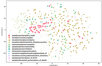
(a)

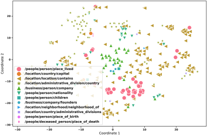
(b)

Figure 1: A 2-D visualization of the embeddings generated by SentenceBERT on the test set of the NYT dataset. The shapes represent the embeddings of sentences in (a) and sub-sentences in (b). Different shapes correspond to different relations used to label the sentences and sub-sentences. A cluster of the same shapes indicates the embeddings of the sentences and sub-sentences expressing the same relation are located close to each other. The clearer boundaries between the clusters of shapes in (b) indicate a better clusterability than the embeddings in (a) in terms of relation labels.

Past effort has been made to explore properties of sentence embeddings. The work in [12] evaluates the predictive ability of sentence embeddings through predictive tasks. Another work in [13] performs a sentence analogy task by evaluating the degree to which lexical analogies are reflected in sentence embeddings. A significant issue in the current studies is that the sentences are mostly simple sentences. It remains to be answered whether lengths and structures of sentences have any impacts on the topology of sentence embedding spaces.

In this paper, we explore the latent structure of the embedding spaces of complex sentences and their sub-sentences with regard to capturing semantic regularities. We leverage the widely-used dataset for the study of relation extraction [14, 15, 16]. The dataset was constructed by distantly aligning relations in Freebase [17] with sentences from the New York Times (NYT) corpus of years 2005-2006. Each sentence in the dataset is labeled by a semantic relation between two entity mentions in the sentence. The data set is well-suited for our study because we can use the entity mentions as anchors to study the embeddings of various sub-sentences. We collect a set of representative sentence embedding methods and apply these methods to the original NYT sentences and various sub-sentences containing the entity mentions. Our goal is to examine whether the embeddings of (sub-)sentences expressing the same semantic relation cluster together. If the clustering signal in the latent structure is strong, unsupervised methods can recognize relations by simply measuring the distances between embedding vectors, which will greatly reduce the bottleneck of collecting labeled training data.

The work we present in this paper shows some methods generate more clusterable embeddings than others. The sentence structures also have effects on the clusterability of resultant embeddings. As an illustration, Figure 1 shows a 2-D visualization of the embedding spaces generated by the SentenceBERT method on the test set of the NYT dataset. The embedding space of the span sub-sentences in Figure 1(b) has better clustering structures than that of the original sentences in Figure 1(a). For reproducibility, all the data and code of the study in this paper are put in a public repository.

The rest of the paper is structured as follows. Section II discusses related work. Section III describes the technical background of the sentence embedding methods. Section IV presents the methods for extracting sub-sentences. Section V describes the analytic methods and experimental process. Section VI presents the experimental results. Section VII discusses the study. Finally, Section VIII concludes the paper.

II Related Work

There is an extensive body of research on exploring properties of word embeddings [18, 1, 19]. The work in [19] applied graph theoretic tools on the semantic networks induced by word embeddings. The study demonstrated that network analysis on word embeddings could draw interesting structures about semantic similarity between words. In contrast, exploring the properties of sentence embeddings has been much more limited. A common approach is to compare the performance of sentence embeddings in various downstream NLP tasks as in [12]. The first task of SemEval 2014 [20, 21] applied and evaluated sentence embeddings in a semantic relatedness task. The authors in [22] evaluated sentence embeddings using a semantic classification task. The RepEval 2017 Shared Task [23, 24] compared seven sentence embedding methods on shared sentence entailment task. The work in [9] performed a comprehensive evaluation of sentence embedding methods using a wide variety of downstream and linguistic feature probing tasks. Another work [25] evaluated several sentence embedding methods, including BERT, InferSent, semantic nets and corpus statistics (SNCS), and Skipthought, by performing a paraphrasing task. All the work attempted to discover the relationships between the geometric structures of embedding spaces and NLP applications.

Our work is closely related to the study of sentence analogy in [13]. Differing from the work, our work evaluates and explores the clustering properies of sentence embeddings with regard to expressing semantic relations between entities. More importantly, our work explores the latent structures of the embeddings of complex sentences and their sub-sentences.

III Sentence Embedding Methods

In this study, we select a set of representative methods that can be classified into 3 categories: word-embedding-aggregation approach, from-scratch-sentence-embedding approach, and pre-trained-fine-tune approach. The classification is based on the guiding principles and algorithms employed by the methods. Here, we briefly describes the technical details of the methods in each category. The public repository contains all implementation code and pointers to the original sources.

Category 1: word-embedding-aggregation:
Method 1. GloVe-Mean [26]: GloVe-Mean takes the arithmetic average of the word embeddings in a sentence as the sentence embedding. As its name indicates, GloVe-Mean uses the pre-trained word embeddings generated by the GloVe method [2]. Let $s=\{w_{1},w_{2},...,w_{n}\}$ be a sentence consisting of a sequence of words, $w_{1}$, $w_{2}$, …, $w_{n}$. Let $\mathbf{v}(w_{i})\in\mathbb{R}^{d}$ be the $d$-dimensional embedding vector of a word $w_{i}$. The GloVe-Mean generates the embedding vector $\mathbf{v}(s)\in\mathbb{R}^{d}$ for the sentence $s$ as:

$$\mathbf{v}(s)=\frac{{\sum}_{i=1}^{n}\mathbf{v}(w_{i})}{n}$$

GloVe-Mean is one of the simplest ways to convert the embeddings of a sequence of words to a single sentence embedding. In our study, we use our own home-grown code for GloVe-Mean.

Method 2. GloVe-DCT [27]: GloVe-Mean treats the words in a sentence as in a bag, ignoring their ordering. To address this, GloVe-DCT stacks individual GloVe word vectors $\mathbf{v}(w_{1})$, $\mathbf{v}(w_{2})$,… , $\mathbf{v}(w_{n})$ into a $n\times d$ matrix. It then applies a discrete cosine transformation (DCT) on the columns. Given a vector of real numbers $c_{0},\ldots,c_{N}$, DCT calculates a sequence of coefficients as follows:

$$coef[0]=\sqrt{\frac{1}{N}}\sum_{n=0}^{N}c_{n}$$

and

$$coef[k]=\sqrt{\frac{2}{N}}\sum_{n=0}^{N}c_{n}\cos\frac{\pi}{N}(n+\frac{1}{2})k$$

The choice of $k$ typically ranges from 1 to 6, where a choice of zero is essentially similar to GloVe-Mean. To get a fixed-length and consistent sentence vector, GloVe-DCT extracts and concatenates the first $K$ DCT coefficients and discards higher-order coefficients. The size of sentence embeddings is $Kd$. In our study, we use our own home-grown code for GloVe-DCT.

Method 3. GloVe-GEM [4]: For a sentence $s=\{w_{1},w_{2},...,w_{n}\}$, GloVe-GEM takes the word embeddings $\{\mathbf{v}(w_{i})\in\mathbb{R}^{d},i=1..n\}$ as input. It generates the sentence embedding $\mathbf{v}(s)$ by a weighted sum

$$\mathbf{v}(s)=\sum_{i=1}^{n}\alpha_{i}\mathbf{v}(w_{i})\quad\mathrm{s.t.}\quad\alpha_{i}=\alpha_{n}+\alpha_{s}+\alpha_{u}$$

where the weights $\alpha_{i},i=1..n$ come from three scores: a novelty score $\alpha_{n}$, a significance score $\alpha_{s}$, and a corpus-wise uniqueness score $\alpha_{u}$. To compute the three scores, GloVe-GEM applies the Gram-Schmidt Process (also known as QR factorization) to the context matrices of the words in the sentence. For each word, its context matrix is made up with the word embeddings in its surrounding context. The method then builds an orthogonal basis of the context matrix. The scores of the word are computed based on principled measures using the bases. Finally, GloVe-GEM removes the sentence-dependent principle components from the weighted sum. In our study, we use our own home-grown code for GloVe-GEM too.

Category 2: from-scratch-sentence-embedding:
Method 4. Skipthought [6]: Inspired by the skip-gram model of word2vec, Skipthought generates sentence embeddings via the task of predicting neighboring sentences. Skipthought depends on a training corpus of contiguous text. It thus uses a large collection of novels, the BookCorpus unlabeled dataset, for training its model. The model is in the encoder-decoder framework. An encoder maps words to a sentence vector and a decoder is used to generate the surrounding sentences. Several choices of encoder-decoder pairs have been explored, including ConvNet-RNN, RNN-RNN, and LSTM-LSTM. In our study, we use the open source implementation of Skipthought.

Method 5. Quickthought [7]: Quickthought also uses the unlabeled BookCorpus for training its model. Instead of reconstructing the surface form of the input sentence or its neighbors, Quickthought uses the embedding of the current sentence to predict the embeddings of neighboring sentences. In particular, given a sentence, Quickthought’s model chooses the correct target sentence from a set of candidate sentences. The model achieves this by replacing the generative objectives with a discriminative approximation. In our study, we use the open source implementation of Quickthought.

Method 6. InferSentV1 and Method 7. InferSentV2 [5]: InferSent uses a three-way classifier to predict the degree of sentence similarity (similar, not similar, neutral). It builds a bi-directional LSTM model pre-trained on natural language inference (NLI) tasks. InferSent comes in two flavors, a V1 model using the pre-trained GloVe vectors and a V2 model using the pre-trained FastText [26] vectors. Individually, we refer to them as InferSentV1 and InferSentV2. In our study, we use the open source implementation of InferSent.

Method 8. LASER [28]: LASER trains a Bi-directional LSTM model on a massive scale, multilingual corpus. It uses parallel sentences accross 93 input languages. LASER is able to focus on mapping semantically similar sentences to close areas of the embedding space. It allows the model to focus more on meaning and less on syntactic features. Each layer of the LASER model is 512 dimensional. By concatenating both the forward and backward representations, LASER generates a final sentence embedding of dimension 1024. In our study, we use the open source implementation of LASER.

Category 3: pre-trained-fine-tune:
Method 9. SentenceBERT [3]: BERT [29] like pre-trained language models have helped many NLP tasks achieve state-of-the-art results. One issue of BERT is that it does not directly generate sentence embeddings. SentenceBERT [3] is a modification of the pre-trained BERT network. It uses siamese and triplet network structures to derive semantically meaningful sentence embeddings. Specifically, SentenceBERT derives a fixed sized sentence embedding by adding a pooling operation to the output of BERT / RoBERTa. The network structure depends on the available training data. A variety of structures and objective functions are tested, including Classification Objective Function, Regression Objective Function, and Triplet Objective Function. In our study, we use the open source implementation of SentenceBERT. In particular, we use the base model “bert-base-nli-mean-tokens”. The model computes the mean of all output vectors of the BERT.

IV Sentence and Sub-Sentence

Sentence segmentation [30] is a non-trivial NLP task that aims to divide text into meaningful component sentences. Automatic sentence segmentation typically divides text based on syntactic structures such as punctuation. The resultant sentences often express multiple ideas with variable lengths. In this study, we examine the strengths and weaknesses of different methods for encoding all valid (sub-)sentences for relation extraction. The validity of a (sub-)sentence means the (sub-)sentence must cover the identified entity mentions.

An entity mention is defined as a span of tokens in a sentence. The following sentence is an example in the NYT dataset. We refer to the sentence as $S1$:
$S1$: “But that spasm of irritation by a master intimidator was minor compared with what Bobby Fischer, the erratic former world chess champion, dished out in March at a news conference in Reykjavik, Iceland.”
The sentence is labeled with the ‘contains’ relation between two geographical locations. The two underlined spans, Reykjavik and Iceland, are identified as the two entity mentions representing two locations.

There are simple sentences such as ”Rechard Levine was born in Manhattan.” It is labeled with the relation ‘place_of_birth’ between the two underlined entity mentions. There are also compound-complex sentences consisting of multiple independent and dependent clauses. The NYT data set contains 372,853 sentences. Out of them, 111,610 sentences are labeled with 24 relations defined in FreeBase [17]. For the labeled sentences, the longest sentence has 265 words, while the shortest sentence has 4 words. The mean length is 39 words. Since we will extract valid sub-sentences to compare to the original sentences, we aimed to make sure that the original sentences are statistically long enough such that the extracted valid sub-sentences are significantly different from the original ones. To this extent, we extracted sub-sentences consisting of the sequence of tokens between the two entity mentions (including the two mentions.) We call such a sub-sentence span. Examining the lengths of spans, we find the longest span has 99 words, while the shortest span has 2 words. The mean length of spans is 11 words. The standard deviation of the sentence lengths is 15 words while the standard deviation of the span lengths is 9 words. The dataset allows us to conduct the study on examining the embedding spaces of sentences and valid sub-sentences with significantly different lengths.

Method Name	Definition
$X_{0}$:span:	extracts the sub-sentence starting from the first mention and ending at the second mention.
$X_{1}$:spanBA1:	extracts the sub-sentence extending 1 token before the span and 1 word after the span.
$X_{2}$:spanBA2:	extracts the sub-sentence extending 2 tokens before the span and 2 words after the span.
…	… …
$X_{10}$:spanBA10:	extracts the sub-sentence extending 10 tokens before the span and 10 words after the span.
$X_{15}$:spanBA15:	extracts the sub-sentence extending 15 tokens before the span and 15 word after the span.
$X_{20}$:spanBA20:	extracts the sub-sentence extending 20 tokens before the span and 20 words after the span.
$Y_{1}$:surroundings1:	extracts the concatenation of the sub-sentences each of which containing 1 token surrounding a mention.
$Y_{2}$:surroundings2:	extracts the concatenation of the sub-sentences each of which containing 2 tokens surrounding a mention.
…	… …
$Y_{10}$:surroundings10:	extracts the concatenation of the sub-sentences each of which containing 10 tokens surrounding a mention.
$Y_{15}$:surroundings15:	extracts the concatenation of the sub-sentences each of which containing 15 tokens surrounding a mention.
$Y_{20}$:surroundings20:	extracts the concatenation of the sub-sentences each of which containing 20 tokens surrounding a mention.

TABLE I: Sub-Sentence Extraction Methods

TABLE I summarizes the extraction methods. Since all valid sub-sentences must contain the identified entity mentions, the extractions anchor on the entity mentions. We also apply extraction of sub-sentences up to length 40, based on the average NYT sentence length of 39 tokens. Starting with the entity mentions, the first method, $X_{0}$:span, extracts the sub-sentence spanning from the first entity mention to the second entity mention. The second method, $X_{1}$:spanBA1, extracts the sub-sentence extending the span with one token before and after the entity mentions. Likewise, $X_{i}$:spanBA$i$, for $i=2...20$, extend the span with $i$ tokens before and after the entity mentions. For instance, from the example sentence $S1$, $X_{0}$:span extracts “Reykjavik, Iceland”, $X_{1}$:spanBA1 extracts “in Reykjavik, Iceland .”, $X_{2}$:spanBA2 extracts “conference in Reykjavik, Iceland .”, and so on. The next group of methods, $Y_{j}$:surroundings$j$, for $j=1...20$, extract the entity mentions and $j$ tokens surrounding the entity mentions. The method $Y_{j}$:surroundings$j$ differs from $X_{i}$:spanBA$i$ in that $Y_{j}$:surroundings$j$ starts from entity mentions and extends on both sides of each mention, while $X_{i}$:spanBA$i$ starts from a span and extends on both sides of the span. The method $Y_{j}$:surroundings$j$ may extract discontinuous chunks from a sentence if the two mentions are located far way from each other in the sentence, and will concatenate the discontinuous chunks as a single sub-sentence. Finally, the methods extract all valid sub-sentences up to length around 40, though the sub-sentences may have duplicates extracted from short original sentences.

V Analytic Design and Experimental Process

There are 9 embedding methods, and 42 sets of original sentences, spans, spanBA1-20, and surroundings1-20. We conduct clustering and network analyses on $9\times 42=378$ embedding spaces generated by the combinations of embedding and sub-sentence extraction methods.

V-A Clustering Analysis

Clustering analysis [31] evaluates the extent to which the sentences expressing the same relations are located in the same partitions. The analysis encompasses two main tasks [32]: (1) clustering tendency assesses whether it is suitable to apply clustering on the embedding spaces in first place, and (2) clustering evaluation seeks to assess the goodness or quality of the clustering given data labels.

Clustering Tendency: The metric we implemented for clustering tendency is Spatial Histogram (SpatHist) [32, 33, 34]. Given a dataset $D$ with $d$ dimensions, we create $b$ equi-width bins along each dimension, and count how many points lie in each of the $b^{d}$ $d$-dimensional cell. We can obtain the empirical joint probability mass function (EPMF) of $D$ based on the binned data. Next, we generate $t$ random samples, each comprising $n$ uniformly generated points within the same $d$-dimensional space as the input data $D$. We can compute the EPMF for each sample too. Finally, we can measure how much the EPMF of the input data $D$ differs from the EPMF of each random sample using the Kullback-Leibler (KL) divergence which is non-negative. The KL divergence is zero when the input data behaves the same as the random sample. The SpatHist is the average of $t$ KL divergences between $D$ and the $t$ random samples. The larger the SpatHist is, the more clusterable the data should be.

Clustering Evaluation. Given a dataset $D$ with partitions $P=\{P_{1},...,P_{m}\}$ each of which has a label, a metric of clustering evaluation measures the extent to which points from the same partition appear in the same cluster, and the extent to which points from different partitions are grouped in different clusters. The higher the metric value is, the better the quality of the clustering. For example, homogeneity [35] quantifies the extent to which a cluster contains entities from only one partition. Suppose the data $D$ is clustered into $k$ groups $C=\{C_{1},C_{2},...,C_{k}\}$. Let $N_{ij}$ be the number of members in group $C_{i}$ with partition label $j$. The homogeneity of the clustering is defined in terms of entropy as: $h=1-\frac{H(C|P)}{H(P)}$, where $H(C|P)$ is the conditional entropy of the clustering $C$ given the partition $P$ and $H(P)$ is the entropy of the original data partitioning. Other metrics apply the same principle but use different ways to measure cluster memberships. We tested the following metrics: purity, fMeasure, Rand Index, homogeneity, mutual information, completeness, vMeasure, and Fowlkes-Mallows measure.

For all the metrics, the higher the value is, the better the clustering quality. Our experiments show that these metrics are consistent in terms of measuring the quality of clustering, though they may be at different value scales.

V-B Network Analysis

For a set of sentence embeddings, we build a Sentence Embedding Similarity Graph (SESG) based on the Euclidean distances between embedding vectors. Given a set of sentences $\mathcal{S}=\{S_{1},S_{2},...,S_{p}\}$, let $\mathbf{W}=\{\mathbf{v}(S_{1}),\mathbf{v}(S_{2}),...,\mathbf{v}(S_{p})\}$ be the set of sentence embeddings. We build the SESG graph corresponding to the sentence embeddings as follows. Let $G=(V,E)$ be the SESG grpah, where $V=\{v_{1},v_{2},....,v_{n}\}$ is the set of vertices, and $E=\{e_{1},e_{2},...,e_{m}\}$ is the set of edges. Initially, the graph $G$ is empty. For a pair of embeddings $\mathbf{v}(S_{i}),\mathbf{v}(S_{j})\in\mathbf{W}$, we add two vertices $v_{i},v_{j}\in V$ and an edge $e_{k}=(v_{i},v_{j})\in E$ between them, if the distance between the embeddings of corresponding sentences is smaller than a threshold, i.e., $||\mathbf{v}(S_{i})-\mathbf{v}(S_{j})||<thresh$. In this study, we choose the threshold as the mean Euclidean distance between the embedding vectors of the sentences that are labeled with the same relations. It should be noted that by cutting off pairs of sentences with larger distances, not every sentence will have a corresponding vertex in the SESG graph.

V-C Experimental Process

Each embedding spaces has 111,160 embedding vectors. We ran the experiments in multiple local and remote compute instances, including 2 local machines each with 16G RAM, 2 virtual machines each with 32G RAM and 8 vCPU in an on-premises cloud, and a Google Colab Pro account. We ran the network analyses using Apache Spark on a Databricks cluster with 8 worker nodes of Amazon m4.large instance.

The sentences in the NYT dataset are labeled by 24 Freebase relations. The sentences labeled with the same relation are considered in the same cluster. To recover the 24 clusters, we apply the K-Means implementation in Scikit-Learn package with $n\_clusters=24$ and other options with the default values. For clustering tendency, we use 500 random samples to average KL divergences for the final SpatHist values. The dimensions of embeddings generated by the 9 embedding methods range from 300 to 4096. The main limitation of the spatial histogram is when we bin each dimension to create cells for computing the EPMF, the number of cells is exponentially large and most of the cells will be empty. To mitigate the problem, we apply a PCA ($n\_component=2$) dimensionality reduction on embedding vectors before we compute the KL divergences.

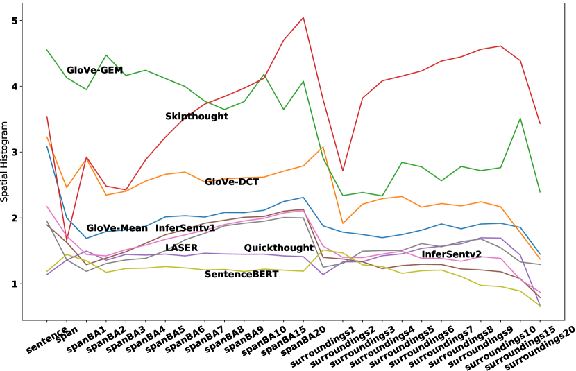
Figure 2: Clustering tendency analysis: Each line represents an embedding method. The x-axis lists the sets of sentences and sub-sentences used to generate the embeddings. The y-axis indicates the values of the metrics (spatial histogram) measuring the clusterability of the embeddings. The higher the y values, the more clusterable the embeddings corresponding to the sets of sentences and sub-sentences on the x-axis.

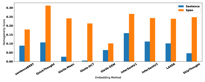
Figure 3: Clustering evaluation analysis: This figure illustrates the clustering evaluation results measured by the homogeneity score metric. It shows the embeddings of the span sub-sentences are more clusterable than that of the original sentences. All metrics demonstrated the same property on different types of sub-sentences. The entire data are available in the github repository.

VI Experimental Results

VI-A Clustering Tendency

Figure 2 shows the results of clustering tendency analysis for the embedding spaces. Each value of the metric (spatial histogram) is computed by averaging 500 KL divergences. Their standard deviations are between $[0.005,0.2]$ with a mean $0.02$. Here are some observations:

• GloVe-GEM generates the most clusterable embeddings on the original sentences and spans with up to 5 extra tokens. The clusterability of the embeddings generated by GloVe-GEM is better than most of the other methods.

• Skipthought generates the most clusterable embeddings on the sub-sentences based on the tokens surrounding entity mentions.

• SentenceBERT and Quickthought generate more clusterable embeddings on spans than on original sentences (the lower-left corner area on the figure).

VI-B Clustering Evaluation

Figure 3 illustrates the clustering evaluation results measured by the homogeneity score metric for the embedding spaces of sentences and spans. It shows the embeddings of the span sub-sentences are more clusterable than that of the original sentences. All metrics demonstrated the same property on different types of sub-sentences. Looking into the entire data set, we have the following key observations:

• Quickthought, GloVe-DCT, GloVe-GEM, and Skip-thought generate the embeddings with better clustering quality on spans than on all other types of sentences.

• SentenceBERT, InferSentV1, InferSentV2, and LASER generate the embeddings with better clustering quality on surroundings1 than on all other types of sentences.

• All of the embeddings generated by the methods from the original sentences are of low clustering quality. Some of them are with the worst clustering quality.

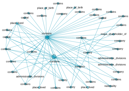
(a)

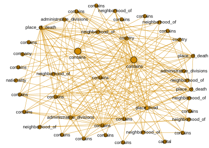
(b)

Figure 4: Visualization of small neighborhood graphs. The vertices correspond to the embeddings of sentences in (a) and sub-sentences in (b). Each vertex is labeled by the relation which is used to label the sentences and sub-sentences. Each neighborhood graph is built around two hubs, i.e., nodes with the highest degree. According to the construction of SESG graph, a hub is close to its neighbors. If the neighbors are also close to each other, we should see dense connection in the neighborhood. The denser the neighborhood graph, the better the clusterability of the embeddings.

VI-C Network Analysis

The potential size of a Sentence Embedding Similarity Graph (SESG) is astronomically large. The number of undirected pairs of sentences is about $111610^{2}/2\approx 6.228\times 10^{9}$. It is infeasible to analyze the SESG graphs for all sets of (sub-)sentences. Because GloVe-GEM has the best performance shown by the clustering analyses, we choose the embeddings generated by GloVe-GEM on the original sentences and spans. We call these two representative SESG graphs GEM-sentence and GEM-span, respectively. Our primary goal is to enrich the findings of clustering analysis through a more focused case study. The final GEM-sentence graph has 94,473 vertices and about $87$ million edges, and the final GEM-span graph has 91,318 vertices and about $104$ million edges. The first observation is that the SESG graph built on span embeddings has more similar pairs than the graph built on sentence embeddings. We measures the density of a graph by the ratio $\frac{number\_of\_edges}{number\_of\_total\_possible\_edges}$. The density of GEM-span is 25% more than the density of GEM-sentence.

The first network analysis is on degree distributions. In both graphs, the degree distributions display a heavy tail. However, there are 543 vertices in GEM-span having the highest degree (=31620), while there are only 25 vertices in GEM-sentence having degrees greater than 31620. It indicates the similarity space of sentences is dominated by a few sentences. We randomly picked up two sentences with the highest degrees. They are “Of Bronxvill, New York.” and “Of Plandome, New York.” Both sentences closely mirror our definition of a span.

The second analysis is about connected components. Both GEM-sentence and GEM-span have a large connected component (CC) with 60% of vertices and more than 99% of edges. About 40% of their vertices fall into other 12,400 in GEM-sentence and 11,500 in GEM-span smaller connected components. The density of the largest CC in GEM-span is 35% more than the density of the largest CC in GEM-sentence. Connected component density increases in comparison to the whole graph.

The third analysis is aimed at the diameter of connected components. It is infeasible to compute the shortest paths between all pairs of vertices in these big graphs ($\sim 10^{9}$). We randomly select 0.1% of the vertices and compute the shortest paths. The longest distance is 8. However, in the random sets from both graphs, more than 87% of the distances are shorter than 3. SESG graphs exhibit small world behavior.

The fourth analysis focuses on the relation distributions in the largest CC. There are 24 relations in the NYT dataset. About 48% of the sentences are labeled as the ‘contains’ relation between two geographical locations. In the largest CC of GEM-sentence, 50% of the vertices corresponding to ‘contains’. In the largest CC of GEM-span, 55% of the vertices corresponding to ’contains’. This shows that $X_{0}$:span improves the quality of the largest cluster of the embeddings.

Finally, we visualize small neighborhoods of the vertices with highest degree in Figure 4. From each graph, we randomly select two vertices (the big dots) with the highest degree. For each selected vertex, we randomly choose about 20 neighbors. The density of the small neighborhood graph from GEM-span in Figure 4 (b) is 16%, while the density of the small neighborhood graph from GEM-sentence in Figure 4 (a) is 10%. The former is denser than the latter one.

VII Discussion

We are motivated by the application of recognizing semantic relations between two entities in a textural sentence. Therefore, using the widely-used data set for relation extraction research in the literature is well-suited for our purpose. Given a set of embedding vectors as a metric space, the distance between any two members, which are usually called points, characterizes the geometric structures of the space. Our analytical methods, specifically clustering and network analyses based on pair-wise distances, reveal a diversity of underlying geometric structures.

Unlike word embedding methods, sentence embedding methods are guided by different underlying principles. However, experimental results show the guiding principles may or may not converge on generating embeddings with similar properties. For example, the embedding spaces generated by SentenceBERT and Quickthought on spans or short segments containing two entity mentions are more clusterable than on the original sentences. It is interesting to note that SentenceBERT and Quickthought share little in terms of their modeling and training processes. It is important to note, however, that both Quickthought and Skipthought share the same principle that uses embeddings to predict the neighboring sentences. But the embedding spaces generated by them exhibit different geometric structures. The values of the clusterability metric in Figure 2 indicate that the methods GloVe-GEM, Skipthought, and GloVe-DCT are the candidates for generating embeddings with better clustering properties in real-world applications.

VIII Conclusion

In this study, we investigate the clusterability of embedding spaces generated by various sentence embedding methods on sentences and different sub-sentences. The primary motivation of the study is that more clusterable embeddings with better clustering quality capture more syntactic and semantic regularities. As a result, downstream NLP applications such as relation extraction would benefit from the embeddings with better clustering quality. We conduct a set of comprehensive clustering and network analyses on the embeddings generated by 9 main embedding methods. The results show that the method GloVe-GEM stands out when applied to the original sentences and spans up to a certain length. Other methods have different strengths on different types of sub-sentences. In most cases, the embeddings generated from the original sentences are of low clustering quality. It signifies the impacts of sentence structures on the quality of embeddings when used by downstream applications. The outcomes of our analysis can be used to aid and direct future sentence embedding models and applications, for example, combining the strengths of different embedding methods.

References

- [1] T. Mikolov, K. Chen, G. S. Corrado, and J. Dean, “Efficient estimation of word representations in vector space,” CoRR, vol. abs/1301.3781, 2013.
- [2] J. Pennington, R. Socher, and C. Manning, “Glove: Global vectors for word representation,” in Proceedings of the 2014 Conference on Empirical Methods in Natural Language Processing (EMNLP), (Doha, Qatar), pp. 1532–1543, Association for Computational Linguistics, Oct. 2014.
- [3] N. Reimers and I. Gurevych, “Sentence-bert: Sentence embeddings using siamese bert-networks,” in Proceedings of the 2019 Conference on Empirical Methods in Natural Language Processing, Association for Computational Linguistics, 11 2019.
- [4] Z. Yang, C. Zhu, and W. Chen, “Parameter-free sentence embedding via orthogonal basis,” in Proceedings of the 2019 Conference EMNLP-IJCNLP, 2018.
- [5] A. Conneau, D. Kiela, H. Schwenk, L. Barrault, and A. Bordes, “Supervised learning of universal sentence representations from natural language inference data,” in Proceedings of the 2017 Conference on Empirical Methods in Natural Language Processing, pp. 670–680, 2017.
- [6] R. Kiros, Y. Zhu, R. Salakhutdinov, R. S. Zemel, A. Torralba, R. Urtasun, and S. Fidler, “Skip-thought vectors,” arXiv preprint arXiv:1506.06726, 2015.
- [7] L. Logeswaran and H. Lee, “An efficient framework for learning sentence representations,” in International Conference on Learning Representations, 2018.
- [8] Z. Chen and J. Ren, “Short text embedding for clustering based on word and topic semantic information,” in 2019 IEEE International Conference on Data Science and Advanced Analytics (DSAA), pp. 61–70, 2019.
- [9] C. S. Perone, R. Silveira, and T. S. Paula, “Evaluation of sentence embeddings in downstream and linguistic probing tasks,” arXiv e-prints, p. arXiv:1806.06259, June 2018.
- [10] J. Li, H. Xu, X. Wang, L. Nie, and X. Xu, “An improved weighted-removal sentence embedding based approach for service recommendation,” in 2020 International Conference on Service Science (ICSS), pp. 44–50, 2020.
- [11] H. Wang, W. Xiong, M. Yu, X. Guo, S. Chang, and W. Y. Wang, “Sentence embedding alignment for lifelong relation extraction,” in Proceedings of the 2019 Conference of the North American Chapter of the Association for Computational Linguistics: Human Language Technologies, (Minneapolis, MN, USA), ACL, 2019.
- [12] Y. Adi, E. Kermany, Y. Belinkov, O. Lavi, and Y. Goldberg, “Fine-grained analysis of sentence embeddings using auxiliary prediction tasks,” in 5th International Conference on Learning Representations, ICLR 2017, 2017.
- [13] X. Zhu and G. de Melo, “Sentence analogies: Linguistic regularities in sentence embeddings,” in Proceedings of the 28th International Conference on Computational Linguistics, pp. 3389–3400, 2020.
- [14] S. Riedel, L. Yao, and A. McCallum, “Modeling relations and their mentions without labeled text,” in ECML PKDD, pp. 148–163, 2010.
- [15] X. Ren, Z. Wu, W. He, M. Qu, C. R. Voss, H. Ji, T. F. Abdelzaher, and J. Han, “Cotype: Joint extraction of typed entities and relations with knowledge bases,” in Proceedings of the 26th International Conference on World Wide Web, pp. 1015–1024, 2017.
- [16] Y. Lin, S. Shen, Z. Liu, H. Luan, and M. Sun, “Neural relation extraction with selective attention over instances,” in Proceedings of the 54th ACL 2016, 2016.
- [17] K. Bollacker, C. Evans, P. Paritosh, T. Sturge, and J. Taylor, “Freebase: a collaboratively created graph database for structuring human knowledge,” in In Proceedings of the 2008 ACM SIGMOD, 2008.
- [18] O. Levy and Y. Goldberg, “Linguistic regularities in sparse and explicit word representations,” in Proceedings of the Eighteenth Conference on Computational Natural Language Learning, pp. 171–180, 2014.
- [19] A. Veremyev, A. Semenov, E. Pasiliao, and et al., “Graph-based exploration and clustering analysis of semantic spaces,” Appl Netw Sci, vol. 4, no. 104, 2019.
- [20] M. Marelli, E. B. annd M. Baroni, R. Bernardi, S. Menini, and R. Zamparelli, “Semeval-2014 task 1: Evaluation of compositional distributional semantic models on full sentences through semantic relatedness and textual entailment,” in In Proceedings of the 8th international workshop on semantic evaluation (SemEval 2014), p. 1–8, 2014.
- [21] N. P. A. Vo, O. Popescu, and T. Caselli, “Fbk-tr: Svm for semantic relatedeness and corpus patterns for rte,” in In Proceedings of the 8th International Workshop on Semantic Evaluation (SemEval 2014), p. 289–293, 2014.
- [22] L. White, R. Togneri, W. Liu, and M. Bennamoun, “How well sentence embeddings capture meaning,” in In Proceedings of the 20th Australasian Document Computing Symposium, ADCS ’15, p. 9:1–9:8, 2015.
- [23] N. Nangia, A. Williams, A. Lazaridou, and S. Bowman, “The rep-eval 2017 shared task: Multi-genre natural language inference with sentence representations,” in In Proceedings of the 2nd Workshop on Evaluating Vector Space Representations for NLP, p. 1–10, 2017.
- [24] H. T. Vu, T.-H. Pham, X. Bai, M. Tanti, L. van der Plas, and A. Gatt, “Lct-malta’s submission to repeval 2017 shared task,” in In Proceedings of the 2nd Workshop on Evaluating Vector Space Representations for NLP, p. 56–60, 2017.
- [25] L. Pragst, W. Minkera, and S. Ultes, “Comparative study of sentence embeddings for contextual paraphrasing,” in Proceedings of the 12th Conference on Language Resources and Evaluation (LREC 2020), p. 6841–6851, 2020.
- [26] A. Joulin, E. Grave, P. Bojanowski, and T. Mikolov, “Bag of tricks for efficient text classification,” CoRR, vol. abs/1607.01759, 2016.
- [27] N. Almarwani, H. Aldarmaki, and M. Diab, “Efficient sentence embedding using discrete cosine transform,” in Proceedings of the 2019 Conference on Empirical Methods in Natural Language Processing and the 9th International Joint Conference on Natural Language Processing (EMNLP-IJCNLP), pp. 3663–3669, 2019.
- [28] M. Artetxe and H. Schwenk, “Massively multilingual sentence embeddings for zero-shot cross-lingual transfer and beyond,” Transactions of the Association for Computational Linguistics, vol. 7, pp. 597–610, 2019.
- [29] J. Devlin, M. Chang, K. Lee, and K. Toutanova, “BERT: pre-training of deep bidirectional transformers for language understanding,” CoRR, vol. abs/1810.04805, 2018.
- [30] D. Dalva, U. Guz, and H. Gurkan, “Effective semi-supervised learning strategies for automatic sentence segmentation,” Pattern Recognition Letters, vol. 105, pp. 76–86, 2018. Machine Learning and Applications in Artificial Intelligence.
- [31] F. I. Vázquez, T. Zseby, and A. Zimek, “Interpretability and refinement of clustering,” in 7th IEEE International Conference on Data Science and Advanced Analytics (DSAA), pp. 21–29, 2020.
- [32] M. J. Zaki and J. Wagner Meira, Data Mining and Machine Learning: Fundamental Concepts and Algorithms (2nd Ed). Cambridge University Press, 2020.
- [33] M. Ackerman and S. Ben-David, “Clusterability: A theoretical study,” in Proceedings of the Twelth International Conference on Artificial Intelligence and Statistics, vol. 5, pp. 1–8, 2009.
- [34] A. Adolfsson, M. Ackerman, and N. C. Brownstein, “To cluster, or not to cluster: An analysis of clusterability methods,” Pattern Recognition, vol. 88, p. 13–26, Apr 2019.
- [35] A. Rosenberg and J. Hirschberg, “V-measure: A conditional entropy-based external cluster evaluation measure,” in EMNLP, 2007.