A Survey of Novae in M83

Abstract

The results of the first synoptic survey of novae in the barred spiral and starburst galaxy, M83 (NGC 5236), are presented. A total of 19 novae and one background supernova were discovered during the course of a nearly seven-year survey comprised of over 200 individual nights of observation between 2012 December 12 and 2019 March 14. After correcting for the limiting magnitude and the spatial and temporal coverage of the survey, the nova rate in M83 was found to be $R=19^{+5}_{-3}$ yr^-1. This rate, when normalized to the $K$-band luminosity of the galaxy, yields a luminosity-specific nova rate, $\nu_{K}=3.0^{+0.9}_{-0.6}\times 10^{-10}$ yr${}^{-1}~{}L_{\odot,K}^{-1}$. The spatial distribution of the novae is found to be more extended than the overall galaxy light suggesting that the observed novae are likely dominated by a disk population. This result is consistent with the observed nova light curves which reveal that the M83 novae are on average more luminous at maximum light and fade faster when compared with novae observed in M31. Generally, the more luminous M83 novae were observed to fade more rapidly, with the complete sample being broadly consistent with a linear Maximum-Magnitude vs Rate of Decline relation.

1 Introduction

Nova eruptions are the result of quasi-periodic thermonuclear runaways (TNRs) on the surfaces of accreting white dwarfs in semidetached binary systems (e.g., see Starrfield et al., 2016, and references therein), with eruptions recurring on timescales as short as a year (Kato et al., 2014). Novae are among the most luminous optical transients known, with absolute magnitudes at the peak of the eruption averaging M${}_{V}\sim-7.5$, and reaching M${}_{V}\sim-10$ for the most luminous systems. As a result, they can be seen to great distances and have been studied in external galaxies for more than a century (e.g., in M31, Ritchey, 1917; Hubble, 1929).

The observed properties of novae are predicted theoretically to depend strongly on the structure of the progenitor binary system. The mass of the white dwarf and the rate of accretion onto its surface are the most important parameters, ultimately determining the ignition mass required to initiate the TNR (e.g., Nomoto, 1982; Townsley & Bildsten, 2005; Kato et al., 2014). Systems with high mass white dwarfs accreting at high rates require the lowest ignition masses, and thus have the shortest recurrence times between successive eruptions. The small ignition masses result in eruptions that eject relatively little mass resulting in a rapid photometric evolution (i.e., they produce “fast” novae).

The mass accretion rate is strongly influenced by the evolutionary state of the companion star, with evolved stars typically transferring mass to the white dwarf at a higher rate compared with systems containing main-sequence companions. The amplitudes of the eruptions are also strongly dependent on the nature of the companion star, being as small as $\sim$5 magnitudes as in the case of the M31 recurrent nova M31N 2008-12a (Darnley et al., 2017), or as large as $\sim$20 mag as was observed for the Galactic nova, V1500 Cyg (Duerbeck, 1987). Finally, it is also thought that the chemical composition of the accreted material may also play an important role in determining the observed properties of nova eruptions (e.g., Starrfield et al., 2016, and references therein).

Given that the nature of the nova eruptions are predicted to depend sensitively on the properties of the progenitor binary, it is reasonable to expect that the observed properties of a novae in a given galaxy might vary with the underlying stellar population. In particular, the specific rate of nova eruptions can be expected to be much higher in a population of novae containing higher mass white dwarfs, where the average recurrence times are relatively short. An early attempt to explore this question was undertaken by Yungelson et al. (1997) who computed population synthesis models that predicted that young stellar populations, which contain on average more massive white dwarfs, should produce nova eruptions at a higher rate compared with older populations. Thus, late-type, low mass galaxies, with a recent history of active star formation were predicted to be more prolific nova producers compared with older, quiescent galaxies.

To date, nova rates have been estimated in well over a dozen galaxies (e.g., see Shafter et al., 2014; Shafter, 2019; Della Valle & Izzo, 2020, and references therein). Taken together, the results do not suggest a simple relationship between a galaxy’s specific nova rate (usually taken to be its $K$-band luminosity-specific rate, $\nu_{K}$) and its dominant stellar population (as reflected by its integrated $B-K$ color). Early work by Ciardullo et al. (1990); Shafter et al. (2000); Williams & Shafter (2004) failed to find any correlation between $\nu_{K}$ and Hubble type; however, della Valle et al. (1994) argued that the bluer, late-type systems such as the Magellanic Clouds and M33, had higher specific nova rates compared with earlier type galaxies. More recently, Shara et al. (2016) and Shafter et al. (2017) have analyzed archival HST imaging data of M87 and made a compelling case that the specific nova rate in this giant elliptical galaxy is at least as high, and perhaps higher, than that found in spiral galaxies and the LMC. Given the uncertainties inherent in measuring extragalactic nova rates, particularly in galaxies other than the Magellanic Clouds (where the rates are relatively well constrained by the Optical Gravitational Lensing Experiment (OGLE, Mróz et al., 2016), it’s fair to say that the question of whether the specific rates vary systematically with the underlying stellar population has yet to be answered definitively.

In an attempt to shed further light on how the underlying stellar population may affect observed nova properties, we have undertaken a multi-year survey of novae in the grand-design spiral M83 (NGC 5236) – also known as the Southern Pinwheel galaxy – a metal-rich, late-type barred spiral galaxy of morphological type SAB(s)c (de Vaucouleurs et al., 1991).

Table 1: Log of Observations

UT Date	Julian Date	Limiting mag
(yr mon day)	(2,450,000+)	($R$)	Notes
2012 12 12.361	6273.861	22.3	1
2012 12 18.368	6279.868	22.7	1
2012 12 22.352	6283.852	22.5	1
2012 12 23.345	6284.845	22.9	1
2012 12 28.314	6289.814	21.8	1

Note. — Table 1 is published in its entirety in the machine-readable format. A portion is shown here for guidance regarding its form and content.

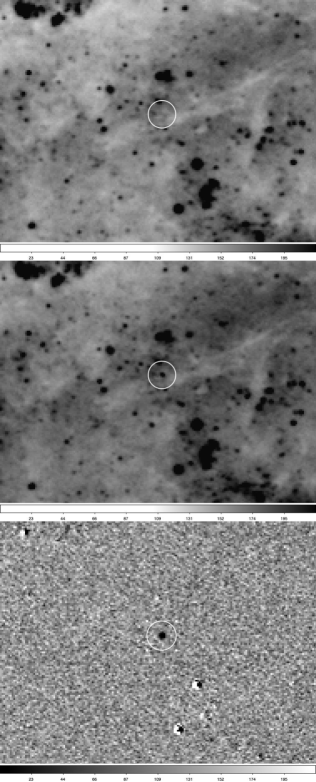
Figure 1: Top panel: A $75^{\prime\prime}\times 57^{\prime\prime}$ portion of a median-combined image from our survey taken on the night of 2014 Feb 11 UT. Middle panel: An image of the same region of the galaxy one month later on 2014 Mar 11 UT. Bottom panel: The difference of the two images as computed by the ISIS image subtraction software, clearly showing the nova M83N 2014-03a.

2 Observations

Our survey for novae in M83 spanned approximately seven years between 2012 December 12 and 2019 March 14. During this time we acquired a total of 205 nightly images of the galaxy. All observations were acquired with the 1.54-m Danish reflector at the La Silla observatory using the DFOSC $2048\times 2048$ CCD imager. The telescope-detector combination resulted in final images covering a square area approximately $13.5^{\prime}$ on a side, with a spatial resolution of 0.396 arcsec pixel^-1. In visual light, M83 has an apparent size of $12.9^{\prime}\times 11.5^{\prime}$, assuring that our observations cover essentially all of the galaxy. However, as described later in section 5.3, the outer halo of M83 may extend slightly beyond our survey’s spatial coverage.

The vast majority of our images were taken through a broad-band $R$ filter, with occasional exposure taken through an $I$ filter. We chose to conduct our primary survey in the $R$-band both because novae develop strong H$\alpha$ emission shortly after eruption, which adds to the flux in the $R$-band, and because the quantum efficiency of the CCD detector reaches a peak near the $R$-band. A complete log of our observations is given in Table 1.

2.1 Image Processing

All images were pipeline processed in the usual manner by first subtracting the bias and dark current, and then flat-fielding the individual images to remove the high-frequency, pixel-to-pixel variations using APHOT (a synthetic aperture photometry and astrometry software developed by M. Velen and P. Pravec at the Ondřejov observatory, Pravec et al., 1994). To eliminate cosmic-ray artifacts in our nightly images, we obtained a series of 120-s images that were later spatially registered and median stacked using SIPS to produce a final image for a given night of observation intended for nova searching. Photometric and astrometric measurements of the novae were done using APHOT on spatially registered and stacked nightly images.

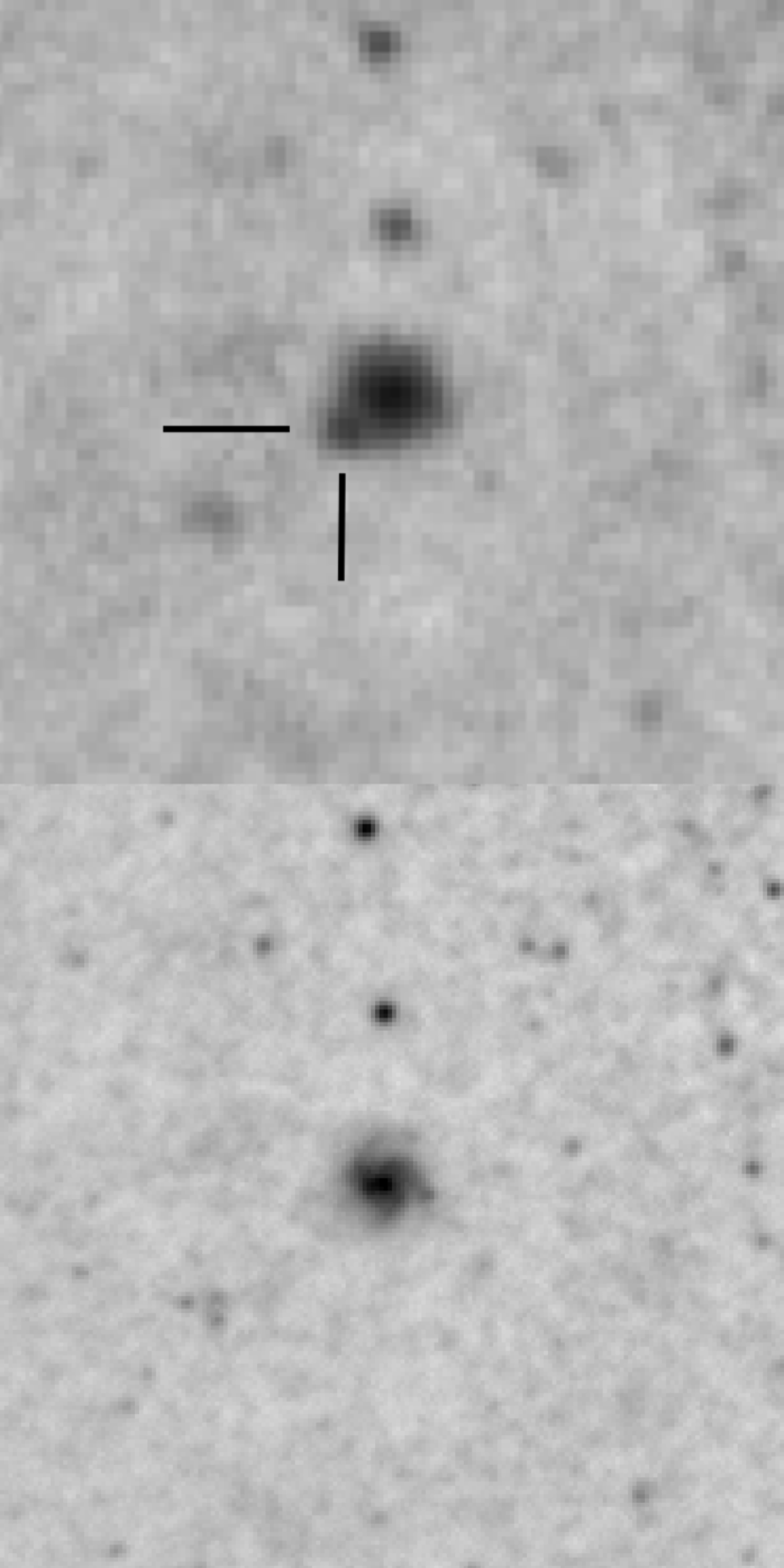
Figure 2: Top panel: A $30^{\prime\prime}\times 30^{\prime\prime}$ portion of our survey image from the night of 2013 Jan 18 UT (North up, East left). The likely supernova is located approximately $2^{\prime\prime}$ E and $1.6^{\prime\prime}$ S of the center of the anonymous spiral galaxy. For comparison, the bottom panel shows an identical $30^{\prime\prime}\times 30^{\prime\prime}$ portion of deep Sloan $r$-band image of the galaxy field taken on 2010 Sep 28 UT by J. L. Prieto using the MEGACAM on the 6.5-m Magellan II - Clay telescope at Las Campanas Observatory.

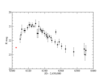
Figure 3: The light curve of the transient source near the anonymous background galaxy. The proximity of the transient source to the galaxy, coupled with the slow rise to maximum light ($\mathrel{\hbox{\hbox to0.0pt{\hbox{\lower 4.0pt\hbox{$\sim$}}\hss}\hbox{$>$}}}10$ d), strongly suggests that the object is a supernova (likely of Type Ia) in the background galaxy, and not a nova in M83. The red triangle represents an upper limit on the flux when the transient was not detected.

Table 2: M83 Novae

		R.A. (2000.0)	Decl. (2000.0)	R.A. offset	Decl. offset
Nova #	Nova name	(h  m  s)	(∘  ′  ′′)	$\Delta\alpha$ cos($\delta$) (′′)	$\Delta\delta$ (′′)	Notes
1	M83N 2013-01a	13 36 44.30	$-29~{}50~{}33.9$	$-216.2$	$82.8$	1
2	M83N 2013-01b	13 37 03.42	$-29~{}53~{}39.8$	$32.5$	$-103.1$	2
3	M83N 2013-01c	13 37 06.75	$-29~{}56~{}15.5$	$75.8$	$-258.8$	3
4	M83N 2013-01d	13 37 10.51	$-29~{}45~{}19.6$	$124.8$	$397.1$	3
5	M83N 2013-03a	13 36 58.76	$-29~{}53~{}22.6$	$-28.1$	$-85.9$	4
6	M83N 2013-04a	13 37 05.80	$-29~{}48~{}11.4$	$63.5$	$225.3$	5
7	M83N 2014-01a	13 37 17.86	$-29~{}53~{}47.7$	$220.3$	$-111.0$	6
8	M83N 2014-01b	13 37 05.81	$-29~{}56~{}02.0$	$63.6$	$-245.3$	3
9	M83N 2014-01c	13 37 15.48	$-29~{}56~{}10.9$	$189.3$	$-254.2$	3
10	M83N 2014-03a	13 37 08.88	$-29~{}50~{}16.6$	$103.6$	$100.1$	7
11	M83N 2015-01a	13 36 35.15	$-29~{}56~{}41.0$	$-335.1$	$-284.3$	8
12	M83N 2015-04a	13 37 08.42	$-29~{}51~{}13.5$	$97.6$	$43.2$	9
13	M83N 2016-02a	13 36 53.01	$-29~{}56~{}19.9$	$-102.8$	$-263.2$	10
14	M83N 2016-02b	13 36 45.52	$-29~{}55~{}57.2$	$-200.2$	$-240.5$	10
15	M83N 2016-03a	13 36 36.15	$-29~{}51~{}44.9$	$-322.2$	$11.8$	11
16	M83N 2018-01a	13 37 09.78	$-29~{}56~{}57.6$	$115.2$	$-300.9$	12
17	M83N 2018-02a	13 37 01.26	$-29~{}55~{}48.2$	$4.4$	$-231.5$	13
18	M83N 2019-02a	13 37 03.82	$-29~{}48~{}21.7$	$37.7$	$215.0$	14
19	M83N 2019-03a	13 37 18.18	$-29~{}48~{}29.0$	$224.6$	$207.7$	15

3 Nova Detection

Novae are transient sources that can be effectively identified through careful comparisons between images from synoptic imaging surveys having a variable cadence such as the one we have conducted. Coarse temporal coverage is sufficient to identify transient sources, but sufficiently dense coverage is required to measure the light curves. The light curves provide assurance that the detected transients are indeed novae and not some other variable objects, such as Luminous Blue Variables (LBVs), or the more common Luminous Red Variables (i.e., Mira variables) that can mimic novae in poorly sampled surveys. Novae can also be distinguished from other variable stars through their $V-I$ color, which is the reason we augmented our data with occasional $I$-band images. The strong H$\alpha$ emission contributing to the $R$-band flux results in a $V-I$ color that is significantly bluer than that of the extremely red Mira variables, which are characterized by $V-I\mathrel{\hbox{\hbox to0.0pt{\hbox{\lower 4.0pt\hbox{$\sim$}}\hss}\hbox{$>$}}}2$ (e.g., see Bhardwaj et al., 2019).

Nova candidates were identified using two different procedures: First, through a direct comparison (blinking) of images from different epochs, and secondly, through a comparison of images from differing epochs using the image subtraction software, ISIS (Alard & Lupton, 1998). Direct comparison of the images proved to be a very effective technique for identifying novae in the outer regions of the galaxy; however, in regions of the galaxy with high surface brightness (i.e., within $\sim 3^{\prime}$ of the nucleus and in some very dense regions of the spiral arms) we had to modify our approach. To detect novae in regions of high background, we first created smoothed (median-filtered) images by sliding a $11\times 11$ pixel box across the image, pixel-by-pixel, replacing the central pixel by the median of all 121 pixels in the box. This median-smoothed image was then subtracted from the original image to produce a median-subtracted image with greatly reduced background variations. These median-subtracted images were once again blinked by eye.

In addition to blinking median-subtracted images, we also employed image subtraction routines from the ISIS image processing package, which increased our sensitivity to novae in regions of high background. Figure 1 shows an example of our ISIS nova detection procedure. The top panel shows a $75^{\prime\prime}\times 57^{\prime\prime}$ portion of a median-combined image from 2014 Feb 11 UT. The middle panel shows an image of the same region of the galaxy one month later on 2014 Mar 11 UT. The nova, M83N 2014-03a, is visible in the March image, and clearly visible in the ISIS subtracted image at the bottom.

We discovered a total of 19 novae over the course of our seven-year survey of M83. Their positions and offsets from the center of M83 (R.A. = $13^{h}37^{m}00.^{s}919$, Decl. = $-29^{\circ}51^{\prime}56.^{\prime\prime}74$, J2000) are given in Table 2. These detections represent the first novae to be reported in M83. It is worth noting that during our inspection of the images we found one transient source located extremely close ($\sim 2^{\prime\prime}$ E and $\sim 1.6^{\prime\prime}$ S) to the center of an anonymous background spiral galaxy (see Figure 2). The background galaxy, which is located at R.A. = $13^{h}~{}37^{m}~{}19.59^{s}$, Decl. = $-29^{\circ}~{}53^{\prime}~{}47.1^{\prime\prime}$, lies $242.3^{\prime\prime}$ E and $110.3^{\prime\prime}$ S from the center of M83. While it is possible that this transient could be a nova in M83, given its proximity to the nucleus of the spiral, we consider it far more likely to have been a supernova in the galaxy discovered serendipitously during the course of our survey (Hornoch et al., 2013). This assessment is backed up by the light curve of the transient (see Figure 3), which shows the relatively slow rise to peak brightness characteristic of supernovae, but not novae. A comparison with the supernova light curve templates given in Doggett & Branch (1985) suggests that the transient is likely a supernova of Type Ia. In view of these considerations, we have excluded this source from our final tally of M83 novae.

3.1 Photometry

Table 3: M83 Nova Photometry

(UT Date)	(JD - 2,450,000)	Mag	Unc.	Band
2013-nova1 = 2013-01a
2012 06 01.138	6079.638	[22.6		R
2012 12 12.361	6273.861	[22.3		R
2012 12 18.368	6279.868	[22.7		R
2012 12 23.345	6284.845	[22.9		R
2012 12 28.314	6289.814	21.0	0.15	R
2012 12 28.316	6289.816	21.1	0.2	I

Note. — Table 3 is published in its entirety in the machine-readable format. A portion is shown here for guidance regarding its form and content.

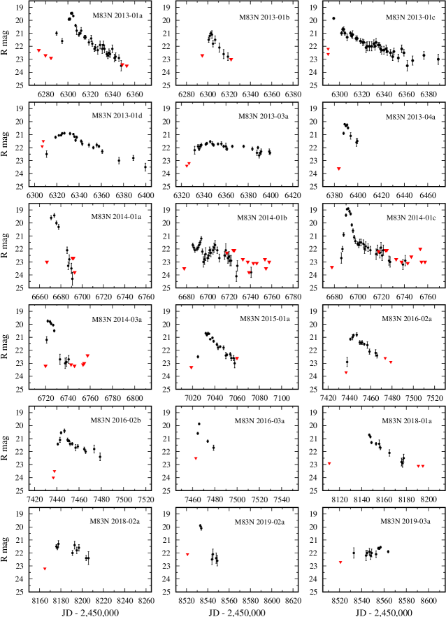
Figure 4: Light curves for 18 of the 19 novae discovered in our survey plotted with consistent axes scales in order to better reveal the relative photometric properties of the novae. The one nova not shown is M83N 2015-04a, where the nova was only seen in one epoch ($R=21.4\pm 0.25$ on JD 2,457,120.915). The red triangles represent upper limits on the flux at times when the novae were not detected.

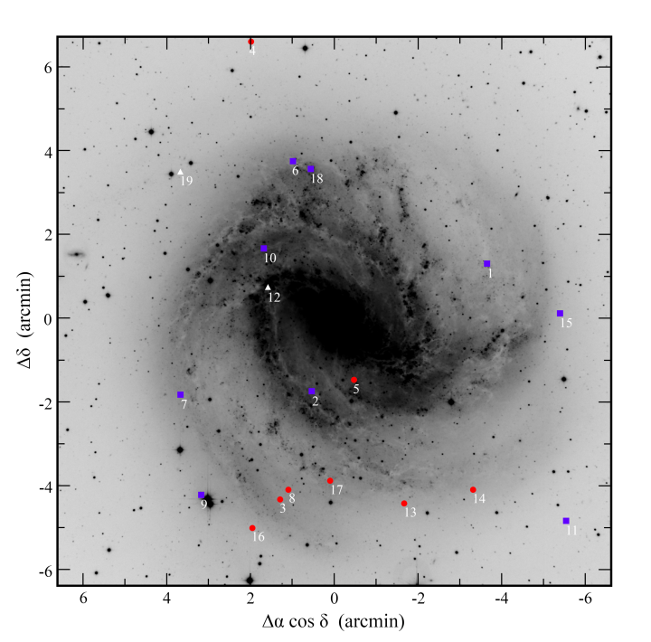
Figure 5: The positions of the 19 novae discovered in our survey superimposed on an image of M83. The blue squares represent relatively “fast” novae with $t_{2}<25$ d, while the red circles show “slow” novae with $t_{2}>25$ d. The white triangles show the two novae without sufficient light curve coverage to determine a rate of decline from peak brightness. We find no correlation between speed class and spatial position within the galaxy, and it is clear that the novae are more spatially extended than is the background galaxy light.

Instrumental magnitudes for all nova candidates were determined by summing the fluxes in 2^′′-in diameter circular apertures in all epochs in which they were visible. Calibrated $R$-band magnitudes were then determined by differential photometry with respect to a set of six secondary standard stars in the M83 field. Both the $R$-band and $I$-band magnitudes of the secondary standard stars were photometrically calibrated by us using the same instrumentation as we used for the survey. As primary standards we used the stars and their magnitudes published in Landolt (1992). We observed both the primary standards and the M83 field during one night under excellent photometric conditions to get properly calibrated the secondary standards in the field of M83 which allow us to obtain photometry of the novae also in non-photometric nights.

The calibrated magnitudes of all 19 novae discovered as part of our survey, on all nights where they were visible, are presented in Table 3. The temporal sampling of our survey was sufficient to produce useful $R$-band light curves for all but one of the 19 novae. The light curves for these 18 novae having multiple epochs of observation are shown in Figure 4. The properties of the light curves (i.e., their peak magnitudes and fade rates) will be explored further in section 6.

4 The Spatial Distribution of M83 Novae

Table 4: M83 Surface Photometry

Semimajor axis	$\Sigma_{R}$		Semimajor axis	$\Sigma_{R}$
(arcsec)	(mag/arcsec2)		(arcsec)	(mag/arcsec2)
0.4	15.90		104.1	20.29
2.7	16.01		107.7	20.25
4.4	16.42		110.7	20.25
7.1	16.98		113.8	20.25
9.3	17.59		117.4	20.25
11.5	17.91		121.8	20.29
13.7	18.17		125.3	20.33
16.3	18.45		128.8	20.38
18.1	18.65		131.5	20.46
20.7	18.80		137.7	20.55
22.1	18.91		142.5	20.61
24.7	18.99		148.2	20.68
25.6	19.06		157.1	20.74
27.4	19.19		165.0	20.85
29.6	19.25		175.6	20.94
31.8	19.30		185.7	21.02
33.5	19.38		199.4	21.18
36.2	19.45		209.1	21.26
38.4	19.51		222.4	21.37
41.0	19.60		236.0	21.50
43.2	19.64		245.3	21.61
46.8	19.68		250.2	21.72
49.9	19.73		259.0	21.74
52.9	19.81		268.2	21.85
56.9	19.86		277.1	21.95
60.9	19.92		287.7	22.11
65.3	19.99		299.1	22.28
69.7	20.03		320.0	22.56
73.2	20.10		350.0	22.96
78.5	20.14		400.0	23.63
86.0	20.20		450.0	24.31
90.4	20.25		500.0	24.98
93.5	20.27		…	…
98.4	20.27		…	…

Figure 5 shows the spatial distribution of the 19 novae discovered in M83 superimposed on a (negative) image of the galaxy. It is immediately apparent that the novae seem to be more spatially extended than the galaxy light. We can explore this impression more quantitatively by comparing the cumulative distribution of the novae with that of the background $R$-band light, as shown in Figure 6. The cumulative background light has been determined by integrating the surface photometry from Table 4, which we have derived from digitizing the radial surface brightness profiles given in Figure 4 of Kuchinski et al. (2000). Since the high surface brightness near the nucleus of the galaxy renders us effectively blind to novae within $\sim 30^{\prime\prime}$ of the center of the galaxy, and likely significantly incomplete within $60^{\prime\prime}$, we have considered three cumulative light distributions starting with inner radii at $R_{\mathrm{i}n}=30^{\prime\prime}$, $R_{\mathrm{i}n}=60^{\prime\prime}$, and $R_{\mathrm{i}n}=90^{\prime\prime}$. Regardless of the adopted inner radius, the cumulative background light clearly falls off faster than the observed nova distribution. This result is formally confirmed by Kolmogorov-Smirnov (K-S) tests ($p=1.6\times 10^{-3}$, $p=3.7\times 10^{-3}$, and $p=1.1\times 10^{-2}$ for cases where we considered inner radii of $R_{in}=30^{\prime\prime}$, $R_{in}=60^{\prime\prime}$, and $R_{in}=90^{\prime\prime}$, respectively), suggesting we can reject the null hypothesis (i.e., the nova and light distributions were drawn from the same parent distribution) with $\mathrel{\hbox{\hbox to0.0pt{\hbox{\lower 4.0pt\hbox{$\sim$}}\hss}\hbox{$>$}}}99\%$ confidence. Thus, it appears that the novae detected in M83 are primarily associated with a more extended disk population of the galaxy.

Before considering possible explanations for why the novae do not appear to follow the overall background light in M83, it is important to rule out the possibility that we may be missing a significant fraction of novae in the inner regions of the galaxy due to the difficulty in detecting them against the high central surface brightness. We explore this possibility below in our determination of the nova rate in M83, which also depends critically on the overall completeness of our survey.

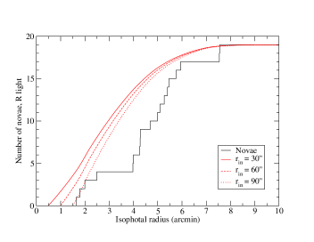
Figure 6: The cumulative distribution of the isophotal radii of the 19 novae (black histogram) compared with the cumulative galaxy $R$-band light for three representative values of the inner radius, $R_{in}$ (shown in red).

5 The Nova Rate in M83

As transient objects, novae are visible for a limited time that depends both on the intrinsic properties of the novae themselves (e.g., their peak luminosities, fade rates, and spatial location within the galaxy) and on parameters inherent to the survey itself; specifically, the temporal sampling and survey depth (the effective limiting magnitude). Whether or not a given nova in M83 can potentially be detected depends on a combination of its peak apparent magnitude, its position within the galaxy, and on the limiting magnitude of our survey images at that location in the galaxy. Then, whether it will actually be detected depends on the time it erupted relative to the dates of our observations and the rate of decline in the nova’s brightness. Given a population of novae with a variety of light curve properties (peak luminosities and fade rates), distributed at different positions within the galaxy, and observed at different times, the only practical way of determining the number of novae we can expect to see in our survey given an intrinsic rate, $R$, is to conduct numerical (Monte Carlo) simulations. Before the simulations can be performed, the first step is to determine the effective completeness of the survey at a given magnitude, $C(m)$.

5.1 The Effective Limiting Magnitude of the Survey

A determination of the limiting magnitude of our survey images is complicated by the fact that the galaxy background surface brightness is highly variable and that the spatial distribution of the novae cannot be assumed to be uniform across the survey images. Thus, no one limiting magnitude can represent the coverage of a given image. We have approached this problem following the procedure described in our earlier work on NGC 2403 (Franck et al., 2012). Specifically, we have conducted artificial nova tests on a representative image (hereafter the fiducial image) under the assumption that the spatial distribution of the artificial novae follows the background light of the galaxy.

The artificial novae were generated using tasks in the IRAF DAOPHOT package, which enabled us to match the point-spread-functions of the real stars in the image. Using the routine addstar, the fiducial image was then seeded with 100 artificial novae having apparent magnitudes randomly distributed within each of a total of eight, 0.5-mag wide, bins. For each of the magnitude bins, the artificial novae were distributed randomly, but with a spatial density that was constrained to follow the integrated background galaxy light of M83. We then searched for the artificial novae using the same procedures that we employed in identifying the real novae. The completeness at the fainter magnitudes was somewhat higher using the ISIS image subtraction analysis, but was generally consistent with the results from a direct comparison of median-subtracted images.

The fraction of novae recovered from the two search techniques in each magnitude bin yielded the completeness functions shown in Figure 7. Given that we discovered the same number of novae in M83 employing both techniques, we have chosen to take the average completeness in a given magnitude bin (the heavy line in Figure 7) to form the basis of the completeness function, $C(m)$. To allow for uncertainty in magnitude bins where the completeness functions differ (the shaded regions), we randomly sample allowed values of $C(m)$ in the analysis to follow. This completeness function can be generalized to any epoch, $i$, of observation by applying a shift, $\Delta m_{i}$ ($=m_{lim,0}-m_{lim,i}$), which represents the difference in the limiting magnitudes (as measured by the faintest star that could be reliably detected near the perimeter of the image away from the galaxy) of our fiducial image and that of the $i$-th epoch image. Thus, for any epoch, $i$, we have $C_{i}(m)=C(m+\Delta m_{i})$.

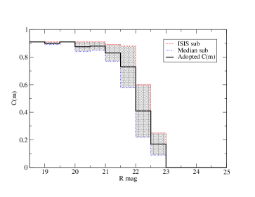
Figure 7: The survey completeness as a function of the $R$-band apparent magnitude, $C(m)$, as determined from our artificial nova tests. The red dashed line shows the completeness from the ISIS image subtraction procedure, the blue dot-dash line shows the completeness using the median-subtraction technique, with the heavy black line shows the average completeness in each magnitude bin. The shaded region shows the range of completeness in each magnitude bin bounded by the two search techniques and used in our Monte Carlo nova rate simulations.

5.2 The Monte Carlo Simulation

As in our earlier extragalactic nova studies (e.g., Franck et al., 2012; Güth et al., 2010; Coelho et al., 2008; Williams & Shafter, 2004), we have employed a Monte Carlo simulation to compute the number of M83 novae that we would expect to observe during the course of our survey.

For a given assumed annual nova rate, $R$, we begin by producing trial novae erupting at random times throughout the time span covered by our survey, each having a peak luminosity and fade rate that has been selected at random from a large sample of known $R$-band light curve parameters. Ideally, we would like to use light curve parameters specific to the full population of M83 novae, but such an unbiased sample does not exist. Instead, we have used the M83 light curve parameters from our observations given in Table 5, augmented with additional $R$-band light curve parameters from the M31 light curves observed by Shafter et al. (2011).

Table 5: Light Curve Parameters

Nova	mR	MR	$f_{R}$	$t_{2}(R)$
(M83N)	(peak)	(peak)	(mag d-1)	(d)
2013-01a	$19.58\pm 0.04$	$-8.90\pm 0.08$	$0.103\pm 0.004$	$19.3\pm 0.7$
2013-01b	$21.11\pm 0.12$	$-7.37\pm 0.14$	$0.115\pm 0.018$	$17.5\pm 2.7$
2013-01c	$20.27\pm 0.06$	$-8.21\pm 0.09$	$0.046\pm 0.002$	$43.2\pm 2.1$
2013-01d	$20.80\pm 0.04$	$-7.69\pm 0.08$	$0.036\pm 0.002$	$54.8\pm 2.9$
2013-03a	$21.66\pm 0.05$	$-6.82\pm 0.08$	$0.013\pm 0.002$	$157.5\pm 21.1$
2013-04a	$20.16\pm 0.05$	$-8.32\pm 0.08$	$0.123\pm 0.015$	$16.3\pm 2.1$
2014-01a	$19.41\pm 0.11$	$-9.08\pm 0.13$	$0.256\pm 0.014$	$7.8\pm 0.4$
2014-01b	$21.68\pm 0.06$	$-6.80\pm 0.09$	$0.033\pm 0.004$	$60.6\pm 7.0$
2014-01c	$18.69\pm 0.05$	$-9.80\pm 0.08$	$0.326\pm 0.012$	$6.1\pm 0.2$
2014-03a	$19.48\pm 0.06$	$-9.00\pm 0.09$	$0.169\pm 0.012$	$11.9\pm 0.9$
2015-01a	$20.63\pm 0.03$	$-7.85\pm 0.08$	$0.085\pm 0.004$	$23.5\pm 1.0$
2016-02a	$20.83\pm 0.07$	$-7.65\pm 0.10$	$0.072\pm 0.008$	$27.7\pm 2.9$
2016-02b	$20.68\pm 0.06$	$-7.80\pm 0.09$	$0.058\pm 0.005$	$34.7\pm 3.1$
2016-03a	$19.90\pm 0.08$	$-8.59\pm 0.11$	$0.157\pm 0.013$	$12.8\pm 1.1$
2018-01a	$20.89\pm 0.05$	$-7.60\pm 0.09$	$0.067\pm 0.006$	$29.9\pm 2.5$
2018-02a	$21.47\pm 0.10$	$-7.01\pm 0.12$	$0.024\pm 0.007$	$83.3\pm 22.6$
2019-02a	$19.91\pm 0.09$	$-8.57\pm 0.11$	$0.181\pm 0.016$	$11.0\pm 1.0$

Adopting a distance modulus to M83 of $\mu_{0}=28.34\pm 0.14$, which represents the mean of the Cepheid and the tip of the red giant branch distances from the recent study by Tully et al. (2016), enables us to compute the expected apparent magnitude distribution at any given epoch, $i$, during our survey, $n_{i}(m,R)$. To account for uncertainty in the distance, our numerical simulations also randomly select values of the distance modulus normally distributed about the mean value. The number of novae expected to be detectable during the course of our survey, $N_{obs}(R)$, can then be computed by convolving the simulated apparent magnitude distribution with the completeness function, $C_{i}(m)$, and then summing over all epochs of observation:

$$N_{\mathrm{o}bs}(R)=\sum_{i}\sum_{m}{C_{i}(m)~{}n_{i}(m,R)}.$$ (1)

The intrinsic nova rate in M83, $R$, and its uncertainty can now be determined through a comparison of the number of novae found in our survey, $n_{\mathrm{o}bs}=19$, with the number of novae predicted by equation (1). We explored trial nova rates ranging from $R=1$ to $R=50$ novae per year, repeating the numerical simulation 10⁵ times for each trial value of $R$. The number of matches, $M(R)$, between the predicted number of observable novae, $N_{obs}(R)$, and the actual number of novae discovered in our survey, $n_{obs}$ = 19, was recorded for each trial value of $R$. The number of matches was then normalized by the total number of matches for all $R$ to give the probability distribution function, $P(R)=M(R)/\sum_{R}{M(R)}$ shown in Figure 8. The most probable nova rate in the portion of the galaxy covered by our survey images is 18${}^{+5}_{-3}$ yr^-1, where the error range (1$\sigma$) for the asymmetrical probability distribution has been computed assuming it can be approximated by a bi-Gaussian function.

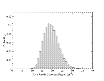
Figure 8: The probability distribution for the nova rate in M83 as determined from our Monte Carlo simulations. The peak of the distribution represents the most likely nova rate in M83. Assuming a bi-Gaussian form for the probability distribution yields a nova rate and associated $1\sigma$ uncertainty of $R_{M83}=18^{+5}_{-3}$ novae per year.

The $K$-band photometry of M83 from the Two-Micron All Sky Survey (2MASS) suggests that the extended halo may extend out to a distance of $r_{tot}\sim 8.5^{\prime}$ from the center of M83. Thus, it is possible that our survey images may be missing a small fraction ($\mathrel{\hbox{\hbox to0.0pt{\hbox{\lower 4.0pt\hbox{$\sim$}}\hss}\hbox{$<$}}}$5%) of the light from the extended halo of M83. Under the assumption that we are sampling $0.95\pm 0.05$ of the total M83 light, we estimate the global nova rate for M83 to be $R_{M83}=19^{+5}_{-3}$ yr^-1.

5.3 The Luminosity-Specific Nova Rate

In order to compare the nova rates between different galaxies or different stellar populations, the rates must first be suitably normalized. Ideally, it would be appropriate to normalize the rates by the mass of stars in the region surveyed, but the mass cannot be measured directly. As a proxy for the mass in stars, it has become standard practice to normalize the nova rate by the infrared $K$-band luminosity of the galaxy. In the case of M83, the integrated apparent $K$-band magnitude as measured by 2MASS is $K=4.62\pm 0.03$. Given the distance modulus, $\mu_{0}=28.34\pm 0.14$, and taking the absolute $K$-band magnitude of the sun to be $M_{K}=3.27\pm 0.02$ (Willmer, 2018), we find that M83 has an absolute magnitude in the $K$-band of $M_{K}=-23.72$, and a corresponding $K$-band luminosity of $(6.32\pm 0.84)\times 10^{10}$ L_⊙,K. Since we estimate that our survey covers $0.95\pm 0.05$ of the entire galaxy where we have found an overall nova rate of $18^{+5}_{-3}$ yr^-1, we arrive at a $K$-band luminosity-specific nova rate for M83 of $\nu_{K}=(3.0^{+0.9}_{-0.6})\times 10^{-10}$ yr^-1 L${}_{K,\odot}^{-1}$.

As recently reviewed by Shafter (2019) and Della Valle & Izzo (2020) prior to the present study, luminosity-specific nova rates had been measured for a total of 15 external galaxies. Figure 9 shows our value of $\nu_{K}$ for M83, along with the values for the other 15 galaxies taken from Table 7.3 in Shafter (2019), plotted as a function of the $B-K$ color of the host galaxy. The specific nova rate for M83 is consistent with those of other spiral galaxies with measured nova rates. As we have noted in previous studies, despite the relatively high $\nu_{K}$ values reported for the Magellanic Clouds and M87 – galaxies with very different Hubble types – there is no compelling evidence that $\nu_{K}$ varies systematically with the underlying stellar population.

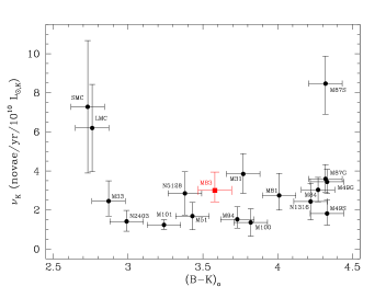
Figure 9: The luminosity-specific nova rates of all 16 galaxies where nova rates are available plotted as a function of the galaxy $B-K$ color. The data have been taken from Table 7.3 of Shafter (2019) with the exception of the value for M83 from the current study, which is shown as a red square.

6 Light Curve Properties

As described in section 3.1, the temporal coverage during the course of our survey was sufficiently dense to enable us to measure $R$-band light curves for 18 of the 19 M83 novae that were detected. These light curves, drawn from an equidistant sample of novae, offer a rare opportunity to explore the relationship between a nova’s peak luminosity and its rate of decline from maximum light, and thus test whether or not the novae obey the canonical (but recently questioned) Maximum-Magnitude versus Rate-of-Decline (MMRD) relation.

6.1 The MMRD Relation

The MMRD relation for novae was first introduced by Mclaughlin (1945), who discovered that the most luminous members of a sample of 30 (mostly Galactic) novae faded more quickly than did their fainter counterparts. He was able to quantify a linear MMRD relation of the form, $M=a+b~{}\mathrm{log}(t_{3})$, where $a$ and $b$ are fitting parameters and $t_{3}$ is the time it takes a nova to fade 3 magnitudes from maximum light (in recent years $t_{2}$, which is more easily measured, is often used as an alternative). Over the years the MMRD relation has been calibrated many times, both in the Galaxy (e.g., Cohen, 1985; Downes & Duerbeck, 2000), and in nearby galaxies such as M31 (e.g., Capaccioli et al., 1989; Shafter et al., 2011), and has often been used as a means for determining the distances to novae where the apparent magnitude at maximum light and the fade rate have been measured.

Over the years it has become increasingly apparent that there is significant scatter in the MMRD, with the existence of the relation itself being called into question, initially by Kasliwal et al. (e.g., 2011) who found that a number of M31 novae observed with the Palomar Transient Factory (PTF) appeared to fall below the canonical MMRD relation (but, see Della Valle & Izzo (2020) for a different interpretation.). Recently, it has become clear that a small subset of novae, typically those with massive white dwarfs that are accreting at high rates (e.g., recurrent novae) fade rapidly despite having relatively low peak luminosities, and thus deviate sharply from the MMRD relation. A good example is the M31 recurrent nova M31N 2008-12a (Darnley et al., 2014; Tang et al., 2014). Given that such systems do in fact exist, it is clear that not all novae will follow a universal MMRD relation. On this basis it has been recently suggested that the notion of an MMRD relation should be abandoned altogether Schaefer (2018). However, the question of whether it is useful to continue to refer to an MMRD relation would seem to depend on the relative frequency of outliers. If the so-called “Faint and Fast” (FFN) novae, such as M31N 2008-12a, are intrinsically rare, then continuing to refer to an MMRD might make sense when considering the behavior of the majority of (non recurrent) novae. On the other hand, if such systems are relatively common, but just missed in most surveys that lack the depth and cadence to discover them, then perhaps the existence of an MMRD relation would be best considered as resulting from an observational selection effect. In either case, it appears that broadly speaking, luminous novae do on average fade more quickly than do their low luminosity counterparts.

Figure 10 shows the MMRD relation for the 17 novae in M83 where the light curves were sufficiently complete to allow a measurement of the peak magnitude and the rate of decline (here measured as $t_{2}$, the time for the nova to fade 2 mags from peak). Although there is significant scatter as expected, there is no question that a general trend, where the more luminous novae fade more quickly, is apparent. The best-fitting linear MMRD relation is given by: $\mathrm{M}_{R}=(-10.79\pm 0.42)+(1.96\pm 0.29)~{}\mathrm{log}~{}t_{2}$. The M31 $R$-band MMRD relation from the study of Shafter et al. (2011) is shown for comparison, and is remarkably similar. Whether or not we are missing a putative population of FFN novae in M83 is unknown. The question can only be answered by future studies having greater depth and cadence, such as those that will be possible with the Large Synoptic Survey Telescope (LSST, Ivezić et al., 2019).

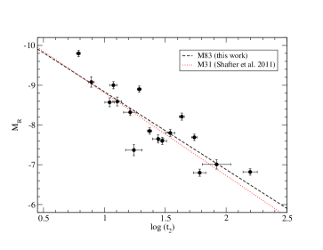
Figure 10: The peak absolute $R$-band magnitudes for the 17 M83 novae with complete light curves are plotted as a function of the log of the fade rate, as measured by the time in days a nova takes to fade by 2 magnitudes in the $R$-band from its peak luminosity, $t_{2}(R)$. The M83 nova sample clearly displays a correlation between peak nova luminosity and $\mathrm{log}(t_{2})$, as shown by the black dashed line. The $R$-band MMRD relation for M31 from Shafter et al. (2011) (red dotted line) is shown for comparison. The two relations are remarkably similar.

6.2 Comparison with the M31 nova population

As part of a comprehensive spectroscopic and photometric survey of novae in M31, Shafter et al. (2011) determined $R$-band light curve parameters for a total of 42 novae and found that, as in the case of M83, the M31 nova sample also generally followed a MMRD relation, albeit with significant scatter (see Table 6 and Figure 19 in Shafter et al., 2011). The M31 novae are characterized by a mean absolute magnitude, $\langle M_{R}\rangle=-7.55\pm 0.14$ and $\langle t_{2}(R)\rangle=38^{+6}_{-5}$ d, while their M83 counterparts from Table 5 yield $\langle M_{R}\rangle=-8.06\pm 0.21$ and $\langle t_{2}(R)\rangle=25^{+6}_{-5}$ d.

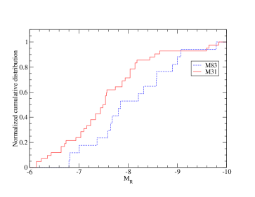
Figure 11: The cumulative distribution of the $R$-band absolute magnitudes of M83 novae compared with their M31 counterparts. A K-S test reveals that the two distributions differ with 94% confidence.

It is interesting to compare the cumulative distributions of the peak luminosities and fade rates from each galaxy, as shown in Figures 11 and 12. The results of K-S tests show that the peak luminosity and fade rate distributions differ between each galaxy with 94% and 74% confidence, respectively. Thus, there is some evidence that the novae in the M83 sample are, on average, more luminous at maximum light and perhaps fade somewhat more rapidly compared with the M31 sample. A possible explanation for this difference is that M31 is an earlier Hubble type galaxy, SA(s)b, and the nova population observed by Shafter et al. (2011) was predominately a bulge population. On the other hand, as discussed earlier, our M83 sample appears to be primarily associated with the galaxy’s disk. Taken together, figures 11 and 12 provide additional support for the existence of two populations of novae, as originally suggested for Galactic systems three decades ago by Duerbeck (1990) and Della Valle & Livio (1998) based on photometric and spectroscopic observations, respectively.

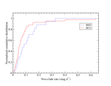
Figure 12: The cumulative distribution of the fade rate of M83 novae in the $R$-band compared with their M31 counterparts. A K-S test reveals that the two distributions differ, but with just 74% confidence.

7 Discussion

7.1 Uncertainty in the Derived Nova Rate

The determination of extragalactic nova rates is challenging, with many sources of uncertainty that must be properly considered in the analysis. Among these, uncertainty in the determination of the survey completeness is perhaps the most important. As described earlier, the completeness – the fraction of novae erupting in the galaxy that can be detected in a given survey – depends quite sensitively on the intrinsic properties of the novae and their actual distribution within the galaxy under investigation. Since neither of these factors are known a priori, assumptions concerning both must always be made.

To guard against potential bias in our M83 nova sample, we chose to include light curve parameters from previous observations of novae in M31 in our Monte Carlo nova rate simulations. As a check on the sensitivity of the final nova rate to the inclusion of the M31 light curve parameters, we have also performed the analysis using only the light curve parameters from the M83 novae discovered in our survey. Despite the differences in the light curve properties between the two samples discussed in the previous section, the final nova rate determination is essentially unchanged (the rate ranges from 17 yr^-1 to 20 yr^-1 when the analysis is restricted to the M83 and M31 light curve parameters, respectively). In this case, the insensitivity of the nova rate to the choice of light curve parameters results from the fact that the M83 novae generally follow an MMRD relation. The M83 novae are on average brighter compared with their M31 counterparts, and thus easier to detect in our simulations, but they fade generally more quickly, so they are observable on average for less time. Thus, the two effects tend to cancel, leaving the final nova rate insensitive to the choice of light curve parameters.

The form of the nova spatial distribution that we have adopted in the artificial nova completeness experiments can also affect the final nova rate computation. In the absence of strong evidence to the contrary, the default approach – and the one we have followed here – is to assume that the spatial density of novae follows the surface brightness of the galaxy (i.e., more light, more novae). However, in the case of M83, it appears that this assumption may be violated. As shown in Figure 5 the observed M83 nova spatial distribution is significantly more extended than the galaxy’s $R$-band light. If this result accurately reflects the intrinsic nova spatial distribution (i.e., we are not missing novae in the inner regions of the galaxy), our artificial nova simulations may underestimate the overall completeness of our survey by placing a greater fraction of the artificial novae in the bright central regions of the galaxy where they are generally more difficult to detect. This bias, although we consider it to be small, would have the effect of slightly overestimating the nova rate determined earlier in our Monte Carlo simulations.

On the other hand, it is worth noting that M83 is an active star-forming galaxy (e.g., see Calzetti et al., 1999), which likely interacted $\sim$1-2 GYr ago with the nearby metal-poor dwarf galaxy, NGC 5253, triggering starbursts in both galaxies (van den Bergh, 1980; Calzetti et al., 1999). The starburst activity in M83 is concentrated in the spiral arms and near the nucleus of the galaxy, which is heavily shrouded in dust (Gallais et al., 1991; Lundgren et al., 2008). These are the same regions of the galaxy where the high surface brightness and complex structure render the detection of novae difficult. Thus, despite our careful nova searches, the possibility that we may be missing some novae in these regions of the galaxy cannot be definitively ruled out. If such a putative population of heavily-extincted novae exists, it would not be properly accounted for by our artificial nova tests, the completeness would be overestimated, and our simulations would then underestimate the true nova rate.

7.2 The Observed Nova Spatial Distribution

As discussed earlier, it was surprising to find that the observed spatial distribution of novae in M83 did not follow the background light of the galaxy. To put this result into context, it is instructive to compare the observed spatial distribution of novae in M83 with similar galaxies for which nova populations have been studied. Such galaxies include the massive, late-type, and nearly face-on spirals M51 and M101 (morphological types SA(s)bc and SAB(rs)cd, respectively), the relatively low-mass, late-type systems NGC 2403 and M33 (SAB(s)cd and SA(s)cd, respectively), and M81, a relatively early-type SA(s)ab spiral with a prominent bulge component. Unfortunately, as we explore below, a review of these studies does not suggest a simple association between the morphological type of the galaxy and the degree to which the nova distribution follows the light of the host galaxy.

In the case of the face-on, grand-design spiral M101 (Shafter et al., 2000; Coelho et al., 2008), the nova density appears to track the background light remarkably well (K-S, p=0.94), while for M33 (Williams & Shafter, 2004; Shafter et al., 2012), the cumulative distributions of the novae and the background light were only marginally consistent (K-S, p=0.4). Similar to our result for M83, the spatial distributions of novae in both M51 (Shafter et al., 2000) and NGC 2403 (Franck et al., 2012), were also found to be more spatially extended than the background light (with 97% and 75% confidence, respectively). In theses cases, however, observational incompleteness in the central region of M51 and the spiral arms of NGC 2403 could possibly explain the discrepancy.

The situation with regard to M81 is more complex. The spatial distribution of novae in this galaxy has been studied extensively by a number of groups, all of whom have come to somewhat different conclusions about how the nova distribution compares with the galaxy light. Based on a total of 15 and 12 detected novae, respectively, Moses & Shafter (1993) and Neill & Shara (2004) argued that the M81 novae most closely follow the galaxy’s bulge light, as was found in several studies of the nova population in M31 (Ciardullo et al., 1987; Shafter et al., 2000; Darnley et al., 2006). More recently, however, Hornoch et al. (2008) analyzed a much larger sample of novae (49) than either of the previous studies, finding that the nova density distribution best matches the overall (bulge + disk) background galaxy light. Given that M81 has a prominent bulge component that dominates the overall light in regions where most novae are found, the apparent discrepancy between these studies may be a distinction without much of a difference. In reviewing the earlier studies in more detail, it appears that neither the Moses & Shafter nor the Neill & Shara data are inconsistent with the hypothesis that the novae follow the overall light.

The only M81 nova study that reached a very different conclusion is that of Shara et al. (1999), who analyzed a sample of 23 novae discovered nearly a half century earlier on Palomar photographic plates taken between 1950 and 1955. They found a significant (disk) population of novae in the outer regions of the galaxy that resulted in a poor fit of the full nova distribution to the overall galaxy light (and clearly a worse fit to the bulge light). The poor fit to the overall light persisted even after the authors attempted to correct their data for missing novae in the inner bulge region of the galaxy. It is not obvious how to reconcile these early photographic data with subsequent CCD studies other than to posit that perhaps an even larger number of bulge novae than expected were missed due to the difficulty in detecting them on photographic plates when projected against the bright background of the galaxy’s bulge.

Taken together, the best evidence currently available suggests that the nova distribution in M81 likely follows the overall background light of the galaxy, with novae belonging to both the bulge and disk populations. In the case of most other galaxies, the situation remains less clear. A combination of small-number statistics, spatial variations in extinction (especially in late-type spiral galaxies), and limited spatial coverage (e.g., in M31) have all conspired to make it difficult to differentiate a real spatial (stellar population) variation from biases caused by observational incompleteness. As is often the case, more data will be required before we have a full and complete understanding of how the nova properties, including their specific rates, vary with the underlying stellar population.

8 Summary

The principal results of our M83 nova survey are as follows:

(1) We have conducted an imaging survey of the SAB(s)c starburst galaxy M83 and discovered a total of 19 novae over the course of our seven-year survey.

(2) After correcting for the survey’s limiting magnitude and spatial and temporal coverage, we find an overall nova rate of $R_{M83}=19^{+5}_{-3}$ yr^-1 for the galaxy.

(3) Adopting an integrated $K$-band magnitude of $K_{M83}=4.62\pm 0.03$ from the 2MASS survey, and a distance modulus for M83 of $(m-M)_{0}=28.34\pm 0.14$, we find the absolute magnitude of M83 in the $K$-band is $M_{K}=-23.72$, which corresponds to a luminosity of $6.32\times 10^{10}$ L_⊙,K. The luminosity-specific nova rate of M83 is then found to be $\nu_{K}=3.0^{+0.9}_{-0.6}\times 10^{-10}$ yr${}^{-1}~{}L_{\odot,K}^{-1}$.

(4) The value of $\nu_{K}$ for M83 is typical of those found for other galaxies with measured nova rates, and, in agreement with our earlier studies, no compelling evidence is found for a variation of $\nu_{K}$ with galaxy color, or Hubble type.

(5) Our survey has enabled us to measure light curves for a total of 18 of the 19 novae discovered in M83. Of these, the peak brightnesses and fade rates ($t_{2}$ times) could be measured for 17 of the novae. These data show that the most luminous novae we observed in M83 generally faded the fastest from maximum light in accordance with the canonical MMRD relation.

(6) We have found the spatial distribution of novae in M83 to be more extended than the background galaxy light suggesting that they are predominately associated with the disk population of the galaxy. In addition, the M83 novae appear, on average, to reach higher luminosities and to evolve more quickly compared with novae in M31, which are predominately associated with that galaxy’s bulge. These findings are consistent with the claim made by Duerbeck (1990), Della Valle & Livio (1998), and others that there are two populations of novae, a “disk” population characterized by generally brighter and faster novae, and a “bulge” population, characterized by novae that are typically slower and less luminous.

Table 1: Log of Observations

UT Date	Julian Date	Limiting mag
yr mon day	(2,450,000+)	($R$)	Notes
2012 12 12.361	6273.861	22.3	1
2012 12 18.368	6279.868	22.7	1
2012 12 22.352	6283.852	22.5	1
2012 12 23.345	6284.845	22.9	1
2012 12 28.314	6289.814	21.8	1
2013 01 02.313	6294.813	21.9	1
2013 01 08.374	6300.874	22.0	1
2013 01 09.370	6301.870	21.7	1
2013 01 10.374	6302.874	22.2	1
2013 01 11.367	6303.867	21.4	1
2013 01 12.374	6304.874	22.4	1
2013 01 14.384	6306.884	21.6	8
2013 01 15.389	6307.889	21.2	6
2013 01 17.368	6309.868	22.9	5
2013 01 18.360	6310.860	23.4	4
2013 01 19.387	6311.887	21.2	3
2013 01 22.373	6314.873	22.6	1
2013 01 23.387	6315.887	22.1	1
2013 01 26.382	6318.882	22.4	2
2013 01 28.389	6320.889	21.9	7
2013 01 29.378	6321.878	23.0	9
2013 01 31.362	6323.862	22.7	10
2013 02 01.308	6324.808	22.6	11
2013 02 03.327	6326.827	22.9	12
2013 02 05.390	6328.890	21.9	1
2013 02 07.397	6330.897	22.2	8
2013 02 08.395	6331.895	22.0	1
2013 02 09.381	6332.881	22.2	10
2013 02 11.387	6334.887	23.0	13
2013 02 12.389	6335.889	23.2	1
2013 02 13.397	6336.897	23.0	1
2013 02 14.398	6337.898	22.6	1
2013 02 16.396	6339.896	22.4	6
2013 02 18.388	6341.888	23.4	1
2013 02 19.385	6342.885	23.3	14
2013 02 20.405	6343.905	22.0	6
2013 02 22.362	6345.862	23.3	11
2013 02 24.349	6347.849	23.0	10
2013 02 25.386	6348.886	23.4	15
2013 03 01.338	6352.838	23.5	11
2013 03 04.397	6355.897	22.6	1
2013 03 06.401	6357.901	23.2	1
2013 03 08.404	6359.904	22.4	1
2013 03 09.404	6360.904	23.5	1
2013 03 14.244	6365.744	23.6	1
2013 03 24.377	6375.877	23.3	1
2012 04 01.240	6383.740	23.6	10
2013 04 05.364	6387.864	23.2	16
2013 04 06.249	6388.749	23.0	15
2013 04 07.301	6389.801	23.2	16
2013 04 08.360	6390.860	22.7	6
2013 04 09.125	6391.625	23.0	1
2013 04 11.422	6393.922	21.4	1
2013 04 16.420	6398.920	22.6	17
2013 04 17.104	6399.604	23.1	1
2013 12 14.349	6640.849	22.7	10
2013 12 15.317	6641.817	22.2	11
2013 12 21.343	6647.843	22.7	19
2013 12 30.367	6656.867	22.4	10
2013 12 31.368	6657.868	23.2	1
2014 01 03.369	6660.869	22.6	1
2014 01 04.369	6661.869	22.8	1
2014 01 08.372	6665.872	22.3	1
2014 01 20.356	6677.856	23.5	11
2014 01 28.379	6685.879	23.0	1
2014 01 29.373	6686.873	23.6	1
2014 01 30.373	6687.873	23.1	1
2014 02 01.368	6689.868	22.7	15
2014 02 02.298	6690.798	23.5	12
2014 02 03.344	6691.844	23.0	16
2014 02 04.391	6692.891	23.8	1
2014 02 05.371	6693.871	23.3	1
2014 02 06.394	6694.894	22.7	1
2014 02 07.399	6695.899	23.0	1
2014 02 08.395	6696.895	22.9	6
2014 02 09.400	6697.900	22.4	6
2014 02 11.346	6699.846	23.4	10
2014 02 12.352	6700.852	23.2	11
2014 02 13.232	6701.732	22.9	11
2014 02 14.311	6702.811	23.0	11
2014 02 16.302	6704.802	22.9	12
2014 02 17.338	6705.838	22.7	10
2014 02 18.322	6706.822	22.5	11
2014 02 20.377	6708.877	22.8	10
2014 02 22.328	6710.828	23.2	19
2014 02 27.261	6715.761	23.5	19
2014 02 28.407	6716.907	22.5	1
2014 03 01.408	6717.908	22.2	1
2014 03 02.407	6718.907	22.4	1
2014 03 03.407	6719.907	22.4	1
2014 03 04.404	6720.904	23.0	1
2014 03 05.409	6721.909	22.6	1
2014 03 07.413	6723.913	22.1	6
2014 03 08.411	6724.911	22.1	1
2014 03 10.319	6726.819	23.5	12
2014 03 11.221	6727.721	23.8	11
2014 03 16.407	6732.907	22.8	1
2014 03 21.057	6737.557	23.0	1
2014 03 22.242	6738.742	23.4	16
2014 03 24.208	6740.708	23.5	19
2014 03 26.331	6742.831	23.1	1
2014 03 29.420	6745.920	23.1	1
2014 04 06.122	6753.622	22.8	12
2014 04 07.161	6754.661	23.5	15
2014 04 10.183	6757.683	23.0	20
2014 12 24.327	7015.827	22.9	19
2014 12 25.355	7016.855	22.8	12
2014 12 27.344	7018.844	22.8	21
2015 01 02.346	7024.846	22.9	21
2015 01 09.351	7031.851	22.7	22
2015 01 10.362	7032.862	22.9	16
2015 01 11.352	7033.852	22.2	10
2015 01 12.345	7034.845	22.8	18
2015 01 13.339	7035.839	23.2	11
2015 01 15.379	7037.879	22.7	1
2015 01 16.375	7038.875	22.7	1
2015 01 19.381	7041.881	22.5	1
2015 01 20.383	7042.883	22.4	1
2015 01 22.349	7044.849	23.2	21
2015 01 25.388	7047.888	22.3	1
2015 01 27.390	7049.890	22.5	1
2015 01 28.374	7050.874	24.6	22
2015 01 31.375	7053.875	23.1	22
2015 02 01.307	7054.807	22.9	18
2015 02 03.376	7056.876	23.1	11
2015 02 04.304	7057.804	23.1	11
2015 02 06.375	7059.875	22.6	18
2015 02 10.329	7063.829	22.4	21
2015 02 12.394	7065.894	22.0	1
2015 02 13.394	7066.894	22.6	1
2015 02 14.396	7067.896	22.7	6
2015 02 17.402	7070.902	22.7	1
2015 02 18.402	7071.902	22.5	1
2015 02 22.378	7075.878	22.9	15
2015 03 03.342	7084.842	23.3	7
2015 03 05.288	7086.788	23.1	23
2015 03 12.407	7093.907	22.5	1
2015 03 13.414	7094.914	21.9	1
2015 03 14.412	7095.912	22.2	1
2015 03 17.413	7098.913	22.1	1
2015 03 19.416	7100.916	21.9	1
2015 03 20.409	7101.909	20.7	6
2015 03 28.422	7109.922	21.5	1
2015 03 31.328	7112.828	22.9	23
2015 04 01.321	7113.821	22.8	23
2015 04 08.415	7120.915	22.4	24
2015 12 15.366	7371.866	21.2	1
2015 12 26.319	7382.819	22.4	21
2016 01 02.322	7389.822	22.8	12
2016 01 11.374	7398.874	22.4	1
2016 01 12.371	7399.871	22.8	1
2016 01 18.365	7405.865	23.2	21
2016 02 01.391	7419.891	22.5	1
2016 02 16.381	7434.881	23.4	23
2016 02 18.391	7436.891	23.9	18
2016 02 19.398	7437.898	23.5	16
2016 02 22.387	7440.887	23.2	16
2016 02 24.406	7442.906	21.2	21
2016 02 25.361	7443.861	22.5	10
2016 02 28.401	7446.901	22.1	19
2016 03 02.216	7449.716	22.5	19
2016 03 03.384	7450.884	23.6	1
2016 03 04.409	7451.909	22.9	1
2016 03 06.395	7453.895	23.8	6
2016 03 09.410	7456.910	22.1	1
2016 03 11.401	7458.901	23.3	21
2016 03 15.415	7462.915	22.5	1
2016 03 17.164	7464.664	22.9	18
2016 03 18.408	7465.908	23.2	25
2016 03 26.120	7473.620	22.6	26
2016 03 31.408	7478.908	22.9	16
2017 12 23.363	8110.863	22.9	1
2018 01 28.263	8146.763	23.3	21
2018 01 29.278	8147.778	22.9	21
2018 01 30.244	8148.744	22.2	12
2018 02 03.360	8152.860	22.8	27
2018 02 06.220	8155.720	22.0	10
2018 02 07.259	8156.759	22.6	21
2018 02 15.397	8164.897	23.0	12
2018 02 26.233	8175.733	23.1	27
2018 02 27.208	8176.708	23.7	27
2018 02 28.200	8177.700	22.3	27
2018 03 13.395	8190.895	23.7	1
2018 03 15.415	8192.515	23.3	1
2018 03 17.409	8194.909	22.8	21
2018 03 19.417	8196.917	21.9	1
2018 03 22.417	8199.917	21.2	1
2018 03 26.207	8203.707	23.1	10
2018 03 28.415	8205.915	23.1	21
2019 01 12.372	8495.872	22.2	1
2019 01 30.388	8513.888	21.9	27
2019 02 04.394	8518.894	21.8	27
2019 02 06.394	8520.894	22.1	27
2019 02 18.399	8532.899	22.2	27
2019 02 19.401	8533.901	22.6	27
2019 03 01.406	8543.906	22.7	1
2019 03 02.282	8544.782	23.5	28
2019 03 04.404	8546.904	22.7	1
2019 03 05.405	8547.905	23.0	1
2019 03 06.405	8548.905	22.9	1
2019 03 10.386	8552.886	22.8	1
2019 03 12.387	8554.887	23.0	1
2019 03 13.406	8555.906	22.9	1
2019 03 14.363	8556.863	23.7	1
2019 03 21.245	8563.745	22.7	27

Table 3: M83 Nova Photometry

(UT Date)	(JD - 2,450,000)	Mag	Unc.	Band
2013-nova1 = 2013-01a
2012 06 01.138	6079.638	[22.6	…	R
2012 12 12.361	6273.861	[22.3	…	R
2012 12 18.368	6279.868	[22.7	…	R
2012 12 23.345	6284.845	[22.9	…	R
2012 12 28.314	6289.814	21.0	0.15	R
2012 12 28.316	6289.816	21.1	0.2	I
2013 01 02.313	6294.813	21.6	0.2	R
2013 01 08.374	6300.874	19.92	0.10	R
2013 01 09.370	6301.870	19.90	0.10	R
2013 01 10.374	6302.874	19.46	0.09	R
2013 01 11.367	6303.867	19.46	0.10	R
2013 01 12.374	6304.874	19.67	0.07	R
2013 01 14.384	6306.884	20.4	0.1	R
2013 01 15.389	6307.889	20.8	0.3	R
2013 01 17.368	6309.868	21.1	0.15	R
2013 01 18.360	6310.860	21.0	0.1	R
2013 01 18.380	6310.880	20.9	0.2	I
2013 01 19.387	6311.887	20.8	0.25	R
2013 01 22.373	6314.873	21.3	0.15	R
2013 01 23.387	6315.887	21.3	0.15	R
2013 01 26.382	6318.882	21.7	0.2	R
2013 01 28.389	6320.889	21.4	0.25	R
2013 01 29.378	6321.878	21.8	0.2	R
2013 01 29.392	6321.892	21.5	0.3	I
2013 01 31.362	6323.862	22.2	0.2	R
2013 02 01.308	6324.808	22.1	0.25	R
2013 02 03.327	6326.827	22.3	0.3	R
2013 02 05.390	6328.890	21.9	0.3	R
2013 02 07.397	6330.897	22.2	0.35	R
2013 02 08.395	6331.895	21.9	0.3	R
2013 02 09.381	6332.881	22.2	0.3	R
2013 02 11.387	6334.887	22.6	0.2	R
2013 02 12.389	6335.889	22.7	0.25	R
2013 02 13.397	6336.897	22.5	0.3	R
2013 02 14.398	6337.898	22.6	0.25	R
2013 02 16.396	6339.896	22.2	0.3	R
2013 02 18.388	6341.888	22.9	0.3	R
2013 02 19.385	6342.885	22.8	0.3	R
2013 02 22.362	6345.862	22.9	0.25	R
2013 02 24.349	6347.849	23.5	0.4	R
2013 02 25.386	6348.886	[23.4	…	R
2013 03 01.338	6352.838	[23.5	…	R
2013-nova2 = 2013-01b
2012 06 01.138	6079.638	[22.8	…	R
2013 01 02.313	6294.813	[22.7	…	R
2013 01 08.374	6300.874	21.5	0.2	R
2013 01 09.370	6301.870	21.2	0.2	R
2013 01 10.374	6302.874	21.0	0.15	R
2013 01 11.367	6303.867	21.1	0.3	R
2013 01 12.374	6304.874	21.8	0.25	R
2013 01 14.384	6306.884	21.5	0.3	R
2013 01 18.360	6310.860	22.1	0.35	R
2013 01 22.373	6314.873	22.6	0.35	R
2013 01 26.382	6318.882	22.8	0.3	R
2013 01 29.378	6321.878	[23.0	…	R
2013-nova3 = 2013-01c
2012 06 01.138	6079.638	[22.8	…	R
2012 12 28.314	6289.814	[22.6	…	R
2012 12 28.316	6289.816	[22.2	…	I
2013 01 02.313	6294.813	19.85	0.09	R
2013 01 09.370	6301.870	21.0	0.15	R
2013 01 10.374	6302.874	20.7	0.15	R
2013 01 11.367	6303.867	20.7	0.2	R
2013 01 12.374	6304.874	21.0	0.15	R
2013 01 14.384	6306.884	21.3	0.25	R
2013 01 17.368	6309.868	21.0	0.15	R
2013 01 18.360	6310.860	21.2	0.15	R
2013 01 19.387	6311.887	21.1	0.3	R
2013 01 22.373	6314.873	21.4	0.2	R
2013 01 23.387	6315.887	21.4	0.2	R
2013 01 26.382	6318.882	21.6	0.2	R
2013 01 28.389	6320.889	21.7	0.25	R
2013 01 29.378	6321.878	21.7	0.2	R
2013 01 29.392	6321.892	21.6	0.35	I
2013 01 31.362	6323.862	22.1	0.4	R
2013 02 01.308	6324.808	22.0	0.35	R
2013 02 03.327	6326.827	22.0	0.35	R
2013 02 05.390	6328.890	22.0	0.35	R
2013 02 07.397	6330.897	21.8	0.3	R
2013 02 08.395	6331.895	22.0	0.3	R
2013 02 09.381	6332.881	21.7	0.3	R
2013 02 11.387	6334.887	21.9	0.2	R
2013 02 12.389	6335.889	21.9	0.2	R
2013 02 13.397	6336.897	22.2	0.3	R
2013 02 14.398	6337.898	22.3	0.3	R
2013 02 16.396	6339.896	22.3	0.3	R
2013 02 18.388	6341.888	22.2	0.3	R
2013 02 19.385	6342.885	22.4	0.3	R
2013 02 22.362	6345.862	22.5	0.25	R
2013 02 24.349	6347.849	22.8	0.3	R
2013 02 25.386	6348.886	22.4	0.25	R
2013 03 01.338	6352.838	22.9	0.3	R
2013 03 04.397	6355.897	22.2	0.3	R
2013 03 06.401	6357.901	22.5	0.25	R
2013 03 09.404	6360.904	23.5	0.4	R
2013 03 14.244	6365.744	23.1	0.35	R
2013 03 24.377	6375.877	22.7	0.3	R
2013 04 06.249	6388.749	23.0	0.4	R
2013 04 17.104	6399.604	[23.3	…	R
2013-nova4 = 2013-01d
2013 01 14.384	6306.884	[21.9	…	R
2013 01 15.389	6307.889	[21.5	…	R
2013 01 18.360	6310.860	22.5	0.25	R
2013 01 18.380	6310.880	[22.6	…	I
2013 01 26.382	6318.882	21.2	0.1	R
2013 01 29.378	6321.878	21.06	0.07	R
2013 01 29.392	6321.892	20.8	0.15	I
2013 01 31.362	6323.862	21.05	0.07	R
2013 02 01.308	6324.808	20.91	0.08	R
2013 02 03.327	6326.827	20.89	0.08	R
2013 02 08.395	6331.895	20.92	0.10	R
2013 02 11.387	6334.887	20.96	0.07	R
2013 02 12.389	6335.889	21.15	0.08	R
2013 02 13.397	6336.897	21.43	0.10	R
2013 02 14.398	6337.898	21.2	0.1	R
2013 02 18.388	6341.888	21.5	0.1	R
2013 02 19.385	6342.885	21.7	0.15	R
2013 02 25.386	6348.886	21.8	0.15	R
2013 03 01.338	6352.838	22.0	0.1	R
2013 03 02.288	6353.788	22.0	0.15	I
2013 03 04.397	6355.897	21.8	0.15	R
2013 03 06.401	6357.901	21.9	0.1	R
2013 03 09.404	6360.904	22.3	0.15	R
2013 03 24.377	6375.877	23.0	0.25	R
2013 04 06.249	6388.749	22.8	0.2	R
2013 04 17.104	6399.604	23.5	0.3	R
2013 04 17.114	6399.614	22.7	0.4	I
2013 12 14.349	6640.849	[23.2	…	R
2013-nova5 = 2013-04a
2012 06 01.138	6079.638	[23.0	…	R
2012 04 01.240	6383.740	[23.6	…	R
2013 04 05.364	6387.864	20.9	0.1	R
2013 04 06.249	6388.749	20.20	0.06	R
2013 04 07.301	6389.801	20.33	0.08	R
2013 04 08.360	6390.860	20.25	0.09	R
2013 04 09.125	6391.625	20.48	0.09	R
2013 04 11.422	6393.922	21.1	0.25	R
2013 04 16.420	6398.920	21.6	0.3	R
2013 04 17.104	6399.604	21.5	0.2	R
2013 04 17.114	6399.614	20.8	0.2	I
2013 12 14.349	6640.849	[22.7	…	R
2013-nova6 = 2013-03a
2013 02 01.308	6324.808	[23.4	…	R
2013 02 03.327	6326.827	[23.2	…	R
2013 02 08.395	6331.895	22.2	0.3	R
2013 02 11.387	6334.887	21.9	0.15	R
2013 02 12.389	6335.889	22.1	0.15	R
2013 02 13.397	6336.897	21.9	0.15	R
2013 02 14.398	6337.898	21.8	0.15	R
2013 02 18.388	6341.888	21.74	0.10	R
2013 02 19.385	6342.885	21.67	0.09	R
2013 02 22.362	6345.862	21.54	0.10	R
2013 02 24.349	6347.849	21.7	0.15	R
2013 02 25.386	6348.886	21.8	0.1	R
2013 03 01.338	6352.838	21.72	0.09	R
2013 03 02.288	6353.788	21.0	0.15	I
2013 03 04.397	6355.897	21.7	0.15	R
2013 03 06.401	6357.901	21.9	0.1	R
2013 03 08.404	6359.904	21.9	0.25	R
2013 03 09.404	6360.904	22.1	0.15	R
2013 03 14.244	6365.744	21.9	0.1	R
2013 03 14.413	6365.913	21.0	0.15	I
2013 03 24.377	6375.877	21.9	0.1	R
2012 04 01.240	6383.740	22.1	0.15	R
2013 04 05.364	6387.864	22.4	0.2	R
2013 04 06.249	6388.749	22.0	0.1	R
2013 04 07.301	6389.801	22.6	0.2	R
2013 04 08.360	6390.860	22.4	0.15	R
2013 04 09.125	6391.625	22.3	0.2	R
2013 04 16.420	6398.920	22.3	0.2	R
2013 04 17.104	6399.604	22.4	0.15	R
2013 04 17.114	6399.614	21.3	0.2	I
2013 12 31.368	6657.868	[23.2	…	R
2014 03 11.221	6727.721	[23.4	…	R
2015 01 28.374	7050.874	[23.8	…	R
2016 02 18.391	7436.891	[23.6	…	R
2018 02 27.208	8176.708	[23.7	…	R
2019 03 14.363	8556.863	[23.6	…	R
2014-nova1 = 2014-01a
2014 01 09.371	6666.871	[23.0	…	R
2014 01 13.360	6670.860	19.60	0.15	R
2014 01 16.271	6673.771	19.42	0.15	R
2014 01 18.282	6675.782	20.0	0.15	R
2014 01 20.356	6677.856	20.30	0.2	R
2014 01 28.379	6685.879	22.1	0.25	R
2014 01 29.373	6686.873	23.3	0.3	R
2014 01 30.373	6687.873	22.8	0.35	R
2014 02 01.368	6689.868	23.5	0.4	R
2014 02 02.298	6690.798	24.3	0.5	R
2014 02 02.307	6690.807	[22.7	…	I
2014 02 03.344	6691.844	[22.7	…	R
2014 02 04.391	6692.891	[23.8	…	R
2014-nova2 = 2014-01b
2014 01 20.356	6677.856	[23.5	…	R
2014 01 28.379	6685.879	21.7	0.15	R
2014 01 29.373	6686.873	21.9	0.15	R
2014 01 30.373	6687.873	22.1	0.15	R
2014 02 01.368	6689.868	22.0	0.15	R
2014 02 02.298	6690.798	21.9	0.15	R
2014 02 02.307	6690.807	21.8	0.2	I
2014 02 03.344	6691.844	21.7	0.2	R
2014 02 04.391	6692.891	21.5	0.15	R
2014 02 05.371	6693.871	21.2	0.15	R
2014 02 06.394	6694.894	22.2	0.2	R
2014 02 07.399	6695.899	23.0	0.4	R
2014 02 08.395	6696.895	22.8	0.4	R
2014 02 09.400	6697.900	22.4	0.5	R
2014 02 11.346	6699.846	22.7	0.25	R
2014 02 12.352	6700.852	22.5	0.25	R
2014 02 13.232	6701.732	22.1	0.25	R
2014 02 14.311	6702.811	22.3	0.3	R
2014 02 16.302	6704.802	22.1	0.3	R
2014 02 17.338	6705.838	21.9	0.35	R
2014 02 18.322	6706.822	21.7	0.35	R
2014 02 20.377	6708.877	22.1	0.25	R
2014 02 22.328	6710.828	22.7	0.3	R
2014 02 27.261	6715.761	22.5	0.3	R
2014 02 28.407	6716.907	22.1	0.5	R
2014 03 01.408	6717.908	[22.3	…	R
2014 03 02.407	6718.907	22.7	0.4	R
2014 03 03.407	6719.907	22.6	0.4	R
2014 03 04.404	6720.904	22.9	0.4	R
2014 03 05.409	6721.909	22.9	0.4	R
2014 03 07.413	6723.913	[22.1	…	R
2014 03 08.411	6724.911	[22.1	…	R
2014 03 10.319	6726.819	24.1	0.4	R
2014 03 11.221	6727.721	23.3	0.4	R
2014 03 16.407	6732.907	[22.8	…	R
2014 03 21.057	6737.557	[23.0	…	R
2014 03 22.242	6738.742	[23.8	…	R
2014 03 24.208	6740.708	23.8	0.4	R
2014 03 26.331	6742.831	[23.1	…	R
2014 03 29.420	6745.920	[23.1	…	R
2014 04 06.122	6753.622	[22.8	…	R
2014 04 07.161	6754.661	[23.5	…	R
2014 04 10.183	6757.683	[23.0	…	R
2014-nova3 = 2014-01c
2014 01 20.356	6677.856	[23.4	…	R
2014 01 28.379	6685.879	22.7	0.4	R
2014 01 29.373	6686.873	22.0	0.2	R
2014 01 30.373	6687.873	20.9	0.15	R
2014 02 01.368	6689.868	19.4	0.1	R
2014 02 02.298	6690.798	18.94	0.07	R
2014 02 02.307	6690.807	18.7	0.15	I
2014 02 03.344	6691.844	18.89	0.07	R
2014 02 04.391	6692.891	19.1	0.1	R
2014 02 05.371	6693.871	19.3	0.1	R
2014 02 06.394	6694.894	20.15	0.1	R
2014 02 07.399	6695.899	20.6	0.15	R
2014 02 08.395	6696.895	21.1	0.15	R
2014 02 09.400	6697.900	21.4	0.2	R
2014 02 11.346	6699.846	21.6	0.15	R
2014 02 12.352	6700.852	21.7	0.2	R
2014 02 13.232	6701.732	21.5	0.25	R
2014 02 14.311	6702.811	21.5	0.25	R
2014 02 16.302	6704.802	21.6	0.3	R
2014 02 17.338	6705.838	22.0	0.35	R
2014 02 18.322	6706.822	21.8	0.35	R
2014 02 20.377	6708.877	21.9	0.3	R
2014 02 22.328	6710.828	22.1	0.3	R
2014 02 27.261	6715.761	22.4	0.4	R
2014 02 28.407	6716.907	22.1	0.4	R
2014 03 01.408	6717.908	[22.2	…	R
2014 03 02.407	6718.907	22.3	0.4	R
2014 03 03.407	6719.907	21.9	0.4	R
2014 03 04.404	6720.904	22.5	0.4	R
2014 03 05.409	6721.909	22.1	0.4	R
2014 03 07.413	6723.913	[22.1	…	R
2014 03 08.411	6724.911	[22.1	…	R
2014 03 10.319	6726.819	22.9	0.35	R
2014 03 11.221	6727.721	23.0	0.4	R
2014 03 16.407	6732.907	[22.8	…	R
2014 03 21.057	6737.557	[23.0	…	R
2014 03 22.242	6738.742	23.2	0.4	R
2014 03 24.208	6740.708	22.9	0.4	R
2014 03 26.331	6742.831	[23.1	…	R
2014 03 29.420	6745.920	[22.6	…	R
2014 04 06.122	6753.622	[22.0	…	R
2014 04 07.161	6754.661	[23.0	…	R
2014 04 10.183	6757.683	[23.0	…	R
2014-nova4 = 2014-03a
2014 03 03.407	6719.907	[23.2	…	R
2014 03 04.404	6720.904	21.2	0.25	R
2014 03 05.409	6721.909	19.75	0.10	R
2014 03 07.413	6723.913	19.8	0.1	R
2014 03 08.411	6724.911	19.95	0.1	R
2014 03 10.319	6726.819	20.06	0.08	R
2014 03 11.221	6727.721	20.5	0.1	R
2014 03 16.407	6732.907	22.7	0.4	R
2014 03 21.057	6737.557	23.0	0.4	R
2014 03 22.242	6738.742	22.9	0.35	R
2014 03 24.208	6740.708	22.7	0.3	R
2014 03 26.331	6742.831	[23.1	…	R
2014 03 29.420	6745.920	[23.2	…	R
2014 04 06.122	6753.622	[23.1	…	R
2014 04 07.161	6754.661	[23.0	…	R
2014 04 10.183	6757.683	[22.4	…	R
2015-nova1 = 2015-01a
2014 12 27.344	7018.844	[23.3	…	R
2015 01 02.346	7024.846	22.5	0.1	R
2015 01 09.351	7031.851	20.69	0.08	R
2015 01 10.362	7032.862	20.82	0.09	R
2015 01 11.352	7033.852	20.7	0.1	R
2015 01 11.354	7033.854	20.4	0.15	I
2015 01 12.345	7034.845	20.73	0.05	R
2015 01 13.339	7035.839	21.15	0.06	R
2015 01 15.379	7037.879	21.04	0.08	R
2015 01 16.375	7038.875	21.30	0.09	R
2015 01 19.381	7041.881	21.55	0.12	R
2015 01 20.383	7042.883	21.8	0.15	R
2015 01 22.349	7044.849	21.72	0.08	R
2015 01 25.388	7047.888	21.8	0.15	R
2015 01 27.390	7049.890	22.4	0.25	R
2015 01 28.374	7050.874	22.35	0.09	R
2015 01 31.375	7053.875	22.3	0.15	R
2015 02 01.307	7054.807	22.6	0.2	R
2015 02 03.376	7056.876	22.6	0.2	R
2015 02 04.304	7057.804	23.0	0.35	R
2015 02 06.375	7059.875	[22.6	…	R
2015-nova2 = 2015-04a
2015 04 01.321	7113.821	[22.8	…	R
2015 04 08.415	7120.915	21.4	0.25	R
2016-nova1 = 2016-02a
2016 02 18.391	7436.891	[23.7	…	R
2016 02 19.398	7437.898	22.9	0.35	R
2016 02 22.387	7440.887	21.14	0.09	R
2016 02 24.406	7442.906	21.0	0.2	R
2016 02 25.361	7443.861	20.84	0.10	R
2016 02 28.401	7446.901	20.8	0.15	R
2016 03 02.216	7449.716	21.4	0.15	R
2016 03 03.384	7450.884	21.44	0.10	R
2016 03 03.401	7450.901	21.5	0.25	I
2016 03 04.409	7451.909	21.4	0.15	R
2016 03 06.395	7453.895	21.53	0.09	R
2016 03 09.410	7456.910	21.6	0.25	R
2016 03 11.401	7458.901	22.1	0.2	R
2016 03 17.164	7464.664	22.2	0.25	R
2016 03 18.408	7465.908	22.4	0.2	R
2016 03 26.120	7473.620	[22.6	…	R
2016 03 31.408	7478.908	[22.9	…	R
2016-nova2 = 2016-02b
2016 02 18.391	7436.891	[24.0	…	R
2016 02 19.398	7437.898	[23.5	…	R
2016 02 22.387	7440.887	21.42	0.09	R
2016 02 24.406	7442.906	21.1	0.2	R
2016 02 25.361	7443.861	20.55	0.10	R
2016 02 28.401	7446.901	20.4	0.15	R
2016 03 02.216	7449.716	21.1	0.15	R
2016 03 03.384	7450.884	21.17	0.09	R
2016 03 03.401	7450.901	20.6	0.1	I
2016 03 04.409	7451.909	21.4	0.15	R
2016 03 06.395	7453.895	21.4	0.1	R
2016 03 09.410	7456.910	21.7	0.25	R
2016 03 11.401	7458.901	21.6	0.15	R
2016 03 17.164	7464.664	21.8	0.15	R
2016 03 18.408	7465.908	22.0	0.15	R
2016 03 26.120	7473.620	21.8	0.3	R
2016 03 31.408	7478.908	22.4	0.3	R
2016-nova3 = 2016-03a
2016 03 15.415	7462.915	[22.5	…	R
2016 03 17.164	7464.664	20.60	0.09	R
2016 03 18.408	7465.908	19.87	0.08	R
2016 03 26.120	7473.620	21.2	0.1	R
2016 03 31.408	7478.908	21.7	0.2	R
2018-nova1 = 2018-01a
2017 12 23.363	8110.863	[22.9	…	R
2018 01 28.263	8146.763	20.71	0.08	R
2018 01 29.278	8147.778	20.86	0.09	R
2018 01 29.290	8147.790	20.7	0.1	I
2018 01 30.244	8148.744	21.3	0.1	R
2018 02 03.360	8152.860	21.4	0.1	R
2018 02 06.220	8155.720	21.4	0.3	R
2018 02 07.259	8156.759	21.7	0.15	R
2018 02 15.397	8164.897	22.1	0.25	R
2018 02 26.233	8175.733	22.8	0.3	R
2018 02 27.208	8176.708	22.9	0.3	R
2018 02 28.200	8177.700	22.5	0.3	R
2018 03 13.395	8190.895	[23.1	…	R
2018 03 17.409	8194.909	[23.1	…	R
2018-nova2 = 2018-02a
2018 02 15.397	8164.897	[23.2	…	R
2018 02 26.233	8175.733	21.5	0.15	R
2018 02 27.208	8176.708	21.6	0.15	R
2018 02 28.200	8177.700	21.3	0.25	R
2018 03 13.395	8190.895	22.0	0.2	R
2018 03 15.415	8192.915	21.4	0.3	R
2018 03 17.409	8194.909	21.8	0.25	R
2018 03 19.417	8196.917	21.6	0.25	R
2018 03 21.417	8198.917	18.5	0.2	Ha
2018 03 26.207	8203.707	22.4	0.2	R
2018 03 28.415	8205.915	22.4	0.5	R
2019-nova1 = 2019-02a
2019 02 06.394	8520.894	[22.1	…	R
2019 02 18.399	8532.899	19.9	0.1	R
2019 02 19.401	8533.901	20.1	0.15	R
2019 03 01.406	8543.906	22.5	0.4	R
2019 03 02.282	8544.782	22.1	0.4	R
2019 03 05.405	8547.905	22.4	0.4	R
2019 03 06.405	8548.905	22.6	0.4	R
2019 03 08.403	8550.903	21.9	0.3	I
2019-nova2 = 2019-03a
2018 03 26.207	8203.707	[24.0	…	R
2019 02 06.394	8520.894	[22.7	…	R
2019 02 18.399	8532.899	22.0	0.4	R
2019 03 01.406	8543.906	22.2	0.4	R
2019 03 02.282	8544.782	22.0	0.2	R
2019 03 04.404	8546.904	21.9	0.25	R
2019 03 05.405	8547.905	22.2	0.3	R
2019 03 06.405	8548.905	22.0	0.3	R
2019 03 08.403	8550.903	21.9	0.3	I
2019 03 10.386	8552.886	22.1	0.25	R
2019 03 12.387	8554.887	21.64	0.09	R
2019 03 13.406	8555.906	21.65	0.09	R
2019 03 14.363	8556.863	21.56	0.08	R
2019 03 21.245	8563.745	21.9	0.1	R
Probable SN in anonymous galaxy in the field of M83
2012 06 01.138	6079.638	[22.8	…	R
2013 01 12.374	6304.874	[22.5	…	R
2013 01 17.368	6309.868	21.9	0.25	R
2013 01 18.360	6310.860	21.6	0.2	R
2013 01 18.380	6310.880	21.6	0.3	I
2013 01 19.387	6311.887	21.2	0.3	R
2013 01 22.373	6314.873	21.3	0.15	R
2013 01 23.387	6315.887	21.3	0.15	R
2013 01 26.382	6318.882	21.1	0.15	R
2013 01 28.389	6320.889	20.9	0.2	R
2013 01 29.378	6321.878	20.9	0.15	R
2013 01 29.392	6321.892	20.5	0.15	I
2013 01 31.362	6323.862	21.0	0.1	R
2013 02 01.308	6324.808	20.9	0.15	R
2013 02 03.327	6326.827	21.0	0.1	R
2013 02 05.390	6328.890	20.8	0.25	R
2013 02 07.397	6330.897	21.5	0.3	R
2013 02 08.395	6331.895	21.5	0.3	R
2013 02 09.381	6332.881	21.0	0.35	R
2013 02 11.387	6334.887	21.2	0.15	R
2013 02 12.389	6335.889	21.3	0.1	R
2013 02 13.397	6336.897	21.4	0.15	R
2013 02 14.398	6337.898	21.3	0.15	R
2013 02 16.396	6339.896	21.5	0.2	R
2013 02 18.388	6341.888	21.6	0.2	R
2013 02 19.385	6342.885	21.7	0.2	R
2013 02 20.404	6343.904	21.8	0.3	R
2013 02 22.362	6345.862	21.7	0.1	R
2013 02 24.349	6347.849	21.8	0.15	R
2013 02 25.386	6348.886	22.0	0.15	R
2013 03 01.338	6352.838	22.1	0.15	R
2013 03 02.288	6353.788	21.4	0.15	R
2013 03 04.397	6355.897	22.3	0.2	R
2013 03 06.401	6357.901	22.1	0.2	R
2013 03 09.404	6360.904	22.4	0.2	R
2013 03 14.244	6365.744	22.6	0.25	R
2013 03 24.377	6375.877	22.8	0.3	R
2013 04 06.249	6388.749	22.6	0.4	R
2013 04 07.301	6389.801	23.0	0.4	R
2013 04 08.360	6390.860	22.7	0.35	R

References

- Alard & Lupton (1998) Alard, C., & Lupton, R. H. 1998, ApJ, 503, 325, doi: 10.1086/305984
- Bhardwaj et al. (2019) Bhardwaj, A., Kanbur, S., He, S., et al. 2019, ApJ, 884, 20, doi: 10.3847/1538-4357/ab38c2
- Calzetti et al. (1999) Calzetti, D., Conselice, C. J., Gallagher, John S., I., & Kinney, A. L. 1999, AJ, 118, 797, doi: 10.1086/300972
- Capaccioli et al. (1989) Capaccioli, M., Della Valle, M., D’Onofrio, M., & Rosino, L. 1989, AJ, 97, 1622, doi: 10.1086/115104
- Ciardullo et al. (1987) Ciardullo, R., Ford, H. C., Neill, J. D., Jacoby, G. H., & Shafter, A. W. 1987, ApJ, 318, 520, doi: 10.1086/165388
- Ciardullo et al. (1990) Ciardullo, R., Ford, H. C., Williams, R. E., Tamblyn, P., & Jacoby, G. H. 1990, AJ, 99, 1079, doi: 10.1086/115397
- Coelho et al. (2008) Coelho, E. A., Shafter, A. W., & Misselt, K. A. 2008, ApJ, 686, 1261, doi: 10.1086/591517
- Cohen (1985) Cohen, J. G. 1985, ApJ, 292, 90, doi: 10.1086/163135
- Darnley et al. (2014) Darnley, M. J., Williams, S. C., Bode, M. F., et al. 2014, A&A, 563, L9, doi: 10.1051/0004-6361/201423411
- Darnley et al. (2006) Darnley, M. J., Bode, M. F., Kerins, E., et al. 2006, MNRAS, 369, 257, doi: 10.1111/j.1365-2966.2006.10297.x
- Darnley et al. (2017) Darnley, M. J., Hounsell, R., Godon, P., et al. 2017, ApJ, 849, 96, doi: 10.3847/1538-4357/aa9062
- de Vaucouleurs et al. (1991) de Vaucouleurs, G., de Vaucouleurs, A., Corwin, Herold G., J., et al. 1991, Third Reference Catalogue of Bright Galaxies
- Della Valle & Izzo (2020) Della Valle, M., & Izzo, L. 2020, A&A Rev., 28, 3, doi: 10.1007/s00159-020-0124-6
- della Valle & Livio (1995) della Valle, M., & Livio, M. 1995, ApJ, 452, 704, doi: 10.1086/176342
- Della Valle & Livio (1998) Della Valle, M., & Livio, M. 1998, ApJ, 506, 818, doi: 10.1086/306275
- della Valle et al. (1994) della Valle, M., Rosino, L., Bianchini, A., & Livio, M. 1994, A&A, 287, 403
- Doggett & Branch (1985) Doggett, J. B., & Branch, D. 1985, AJ, 90, 2303, doi: 10.1086/113934
- Downes & Duerbeck (2000) Downes, R. A., & Duerbeck, H. W. 2000, AJ, 120, 2007, doi: 10.1086/301551
- Duerbeck (1987) Duerbeck, H. W. 1987, Space Sci. Rev., 45, 1, doi: 10.1007/BF00187826
- Duerbeck (1990) —. 1990, Galactic Distribution and Outburst Frequency of Classical Novae, ed. A. Cassatella & R. Viotti, Vol. 369, 34, doi: 10.1007/3-540-53500-4_90
- Franck et al. (2012) Franck, J. R., Shafter, A. W., Hornoch, K., & Misselt, K. A. 2012, ApJ, 760, 13, doi: 10.1088/0004-637X/760/1/13
- Gallais et al. (1991) Gallais, P., Rouan, D., Lacombe, F., Tiphene, D., & Vauglin, I. 1991, A&A, 243, 309
- Güth et al. (2010) Güth, T., Shafter, A. W., & Misselt, K. A. 2010, ApJ, 720, 1155, doi: 10.1088/0004-637X/720/2/1155
- Hornoch (2013a) Hornoch, K. 2013a, The Astronomer’s Telegram, 4723, 1
- Hornoch (2013b) —. 2013b, The Astronomer’s Telegram, 4732, 1
- Hornoch & Kucakova (2018) Hornoch, K., & Kucakova, H. 2018, The Astronomer’s Telegram, 11443, 1
- Hornoch & Kucakova (2019) —. 2019, The Astronomer’s Telegram, 12539, 1
- Hornoch et al. (2019) Hornoch, K., Kucakova, H., & Kurfurst, P. 2019, The Astronomer’s Telegram, 12564, 1
- Hornoch & Paunzen (2018) Hornoch, K., & Paunzen, E. 2018, The Astronomer’s Telegram, 11240, 1
- Hornoch et al. (2008) Hornoch, K., Scheirich, P., Garnavich, P. M., Hameed, S., & Thilker, D. A. 2008, A&A, 492, 301, doi: 10.1051/0004-6361:200809592
- Hornoch et al. (2013) Hornoch, K., Zasche, P., & Wolf, M. 2013, The Astronomer’s Telegram, 4747, 1
- Hubble (1929) Hubble, E. P. 1929, ApJ, 69, 103, doi: 10.1086/143167
- Ivezić et al. (2019) Ivezić, Ž., Kahn, S. M., Tyson, J. A., et al. 2019, ApJ, 873, 111, doi: 10.3847/1538-4357/ab042c
- Kasliwal et al. (2011) Kasliwal, M. M., Cenko, S. B., Kulkarni, S. R., et al. 2011, ApJ, 735, 94, doi: 10.1088/0004-637X/735/2/94
- Kato et al. (2014) Kato, M., Saio, H., Hachisu, I., & Nomoto, K. 2014, ApJ, 793, 136, doi: 10.1088/0004-637X/793/2/136
- Kuchinski et al. (2000) Kuchinski, L. E., Freedman, W. L., Madore, B. F., et al. 2000, ApJS, 131, 441, doi: 10.1086/317371
- Landolt (1992) Landolt, A. U. 1992, AJ, 104, 340, doi: 10.1086/116242
- Lundgren et al. (2008) Lundgren, A. A., Olofsson, H., Wiklind, T., & Beck, R. 2008, in Astronomical Society of the Pacific Conference Series, Vol. 390, Pathways Through an Eclectic Universe, ed. J. H. Knapen, T. J. Mahoney, & A. Vazdekis, 144
- Mclaughlin (1945) Mclaughlin, D. B. 1945, PASP, 57, 69, doi: 10.1086/125689
- Moses & Shafter (1993) Moses, R. N., & Shafter, A. W. 1993, in American Astronomical Society Meeting Abstracts, Vol. 182, American Astronomical Society Meeting Abstracts #182, 85.05
- Mróz et al. (2016) Mróz, P., Udalski, A., Poleski, R., et al. 2016, ApJS, 222, 9, doi: 10.3847/0067-0049/222/1/9
- Neill & Shara (2004) Neill, J. D., & Shara, M. M. 2004, AJ, 127, 816, doi: 10.1086/381484
- Nomoto (1982) Nomoto, K. 1982, ApJ, 253, 798, doi: 10.1086/159682
- Pravec et al. (1994) Pravec, P., Hudec, R., Soldán, J., Sommer, M., & Schenkl, K. H. 1994, Experimental Astronomy, 5, 375, doi: 10.1007/BF01583708
- Prieto & Morrell (2013) Prieto, J. L., & Morrell, N. 2013, The Astronomer’s Telegram, 4734, 1
- Ritchey (1917) Ritchey, G. W. 1917, PASP, 29, 210, doi: 10.1086/122638
- Schaefer (2018) Schaefer, B. E. 2018, MNRAS, 481, 3033, doi: 10.1093/mnras/sty2388
- Schlafly & Finkbeiner (2011) Schlafly, E. F., & Finkbeiner, D. P. 2011, ApJ, 737, 103, doi: 10.1088/0004-637X/737/2/103
- Shafter (2019) Shafter, A. W. 2019, Extragalactic Novae; A historical perspective, doi: 10.1088/2514-3433/ab2c63
- Shafter et al. (2000) Shafter, A. W., Ciardullo, R., & Pritchet, C. J. 2000, ApJ, 530, 193, doi: 10.1086/308349
- Shafter et al. (2014) Shafter, A. W., Curtin, C., Pritchet, C. J., Bode, M. F., & Darnley, M. J. 2014, in Astronomical Society of the Pacific Conference Series, Vol. 490, Stellar Novae: Past and Future Decades, ed. P. A. Woudt & V. A. R. M. Ribeiro, 77. https://arxiv.org/abs/1307.2296
- Shafter et al. (2012) Shafter, A. W., Darnley, M. J., Bode, M. F., & Ciardullo, R. 2012, ApJ, 752, 156, doi: 10.1088/0004-637X/752/2/156
- Shafter et al. (2017) Shafter, A. W., Kundu, A., & Henze, M. 2017, Research Notes of the American Astronomical Society, 1, 11, doi: 10.3847/2515-5172/aa9847
- Shafter et al. (2011) Shafter, A. W., Darnley, M. J., Hornoch, K., et al. 2011, ApJ, 734, 12, doi: 10.1088/0004-637X/734/1/12
- Shara et al. (1999) Shara, M. M., Sandage, A., & Zurek, D. R. 1999, PASP, 111, 1367, doi: 10.1086/316449
- Shara et al. (2016) Shara, M. M., Doyle, T. F., Lauer, T. R., et al. 2016, ApJS, 227, 1, doi: 10.3847/0067-0049/227/1/1
- Starrfield et al. (2016) Starrfield, S., Iliadis, C., & Hix, W. R. 2016, PASP, 128, 051001, doi: 10.1088/1538-3873/128/963/051001
- Tang et al. (2014) Tang, S., Bildsten, L., Wolf, W. M., et al. 2014, ApJ, 786, 61, doi: 10.1088/0004-637X/786/1/61
- Tody (1986) Tody, D. 1986, in Society of Photo-Optical Instrumentation Engineers (SPIE) Conference Series, Vol. 627, Instrumentation in astronomy VI, ed. D. L. Crawford, 733, doi: 10.1117/12.968154
- Townsley & Bildsten (2005) Townsley, D. M., & Bildsten, L. 2005, ApJ, 628, 395, doi: 10.1086/430594
- Tully et al. (2016) Tully, R. B., Courtois, H. M., & Sorce, J. G. 2016, AJ, 152, 50, doi: 10.3847/0004-6256/152/2/50
- van den Bergh (1980) van den Bergh, S. 1980, PASP, 92, 122, doi: 10.1086/130631
- Williams & Shafter (2004) Williams, S. J., & Shafter, A. W. 2004, ApJ, 612, 867, doi: 10.1086/422833
- Willmer (2018) Willmer, C. N. A. 2018, ApJS, 236, 47, doi: 10.3847/1538-4365/aabfdf
- Yungelson et al. (1997) Yungelson, L., Livio, M., & Tutukov, A. 1997, ApJ, 481, 127, doi: 10.1086/304020