Sparse Deep Learning: A New Framework Immune to Local Traps and Miscalibration

Abstract

Deep learning has powered recent successes of artificial intelligence (AI). However, the deep neural network, as the basic model of deep learning, has suffered from issues such as local traps and miscalibration. In this paper, we provide a new framework for sparse deep learning, which has the above issues addressed in a coherent way. In particular, we lay down a theoretical foundation for sparse deep learning and propose prior annealing algorithms for learning sparse neural networks. The former has successfully tamed the sparse deep neural network into the framework of statistical modeling, enabling prediction uncertainty correctly quantified. The latter can be asymptotically guaranteed to converge to the global optimum, enabling the validity of the down-stream statistical inference. Numerical result indicates the superiority of the proposed method compared to the existing ones.

Keywords: Asymptotic Normality, Posterior Consistency, Prior Annealing, Structure Selection, Uncertainty Quantification

1 Introduction

During the past decade, deep neural networks (DNNs) have achieved the state-of-the-art performance in many machine learning tasks such as computer vision and natural language processing. However, the DNN suffers from a training-prediction dilemma from the perspective of statistical inference: A small DNN model can be well calibrated, but tends to get trapped into a local optimum; on the other hand, an over-parameterized DNN model can be easily trained to a global optimum (with zero training loss), but tends to be miscalibrated (Guo et al., 2017). In consequence, it is often unclear whether a DNN is guaranteed to have a desired property after training instead of getting trapped into an arbitrarily poor local minimum, or whether its decision/prediction is reliable. This difficulty makes the trustworthiness of AI highly questionable.

To resolve this difficulty, researchers have attempted from two sides of the training-prediction dilemma. Towards understanding the optimization process of the DNN training, a line of researches have been done. For example, Gori and Tesi (1992) and Nguyen and Hein (2017) studied the training loss surface of over-parameterized DNNs. They showed that for a fully connected DNN, almost all local minima are globally optimal, if the width of one layer of the DNN is no smaller than the training sample size and the network structure from this layer on is pyramidal. Recently, Allen-Zhu et al. (2019); Du et al. (2019); Zou et al. (2020) and Zou and Gu (2019) explored the convergence theory of the gradient-based algorithms in training over-parameterized DNNs. They showed that the gradient-based algorithms with random initialization can converge to global minima provided that the width of the DNN is polynomial in training sample size.

To improve calibration of the DNN, different methods have been developed, see e.g., Monte Carlo dropout (Gal and Ghahramani, 2016) and deep ensemble (Lakshminarayanan et al., 2017). However, these methods did not provide a rigorous study for the asymptotic distribution of the DNN prediction and thus could not correctly quantify its uncertainty. Recently, researchers have attempted to address this issue with sparse deep learning. For example, for Bayesian sparse neural networks, Liang et al. (2018), Polson and Ročková (2018) and Sun et al. (2021) established the posterior consistency, and Wang and Rocková (2020) further established the Bernstein-von Mises (BvM) theorem for linear and quadratic functionals. The latter guarantees in theory that the Bayesian credible region has a faithful frequentist coverage. However, since the theory by Wang and Rocková (2020) does not cover the point evaluation functional, the uncertainty of the DNN prediction still cannot be correctly quantified. Moreover, their theory is developed with the spike-and-slab prior (i.e., each weight or bias of the DNN is subject to a spike-and-slab prior), whose discrete nature makes the resulting posterior distribution extremely hard to simulate. To facilitate computation, Sun et al. (2021) employed a mixture Gaussian prior. However, due to nonconvexity of the loss function of the DNN, a direct MCMC simulation still cannot be guaranteed to converge to the right posterior distribution even with the mixture Gaussian prior.

In this paper, we provide a new framework for sparse deep learning, which successfully resolved the training-prediction dilemma. In particular, we propose two prior annealing algorithms, one from the frequentist perspective and one from the Bayesian perspective, for learning sparse neural networks. The algorithms start with an over-parameterized deep neural network and then have its structure gradually sparsified. We provide a theoretical guarantee that the training procedures are immune to local traps, the resulting sparse structures are consistent, and the predicted values are asymptotically normally distributed. The latter enables the prediction uncertainty correctly quantified. Our contribution in this paper is two-fold:

• We provide a new framework for sparse deep learning, which is immune to local traps and miscalibration.

• We lay down the theoretical foundation for how to make statistical inference with sparse deep neural networks.

The remaining part of the paper is organized as follows. Section 2 lays down the theoretical foundation for sparse deep learning. Section 3 describes the proposed prior annealing algorithms. Section 4 presents some numerical results. Section 5 concludes the paper.

2 Theoretical Foundation for Sparse Deep Learning

As mentioned previously, sparse deep learning has received much attention as a promising way for addressing the miscalibration issue of the DNN. Theoretically, the approximation power of the sparse DNN has been studied for various classes of functions (Schmidt-Hieber, 2017; Bölcskei et al., 2019). Under the Bayesian setting, posterior consistency has been established in Liang et al. (2018); Polson and Ročková (2018); Sun et al. (2021). In particular, the work Sun et al. (2021) has achieved important progress toward taming sparse DNNs into the framework of statistical modeling. They provide a neural network approximation theory fundamentally different from the existing ones. In the existing theory, no data is involved and a small network can potentially achieve an arbitrarily small approximation error by allowing connection weights to take values in an unbounded spacemaiorov1999lower. In contrast, the theory by Sun et al. (2021) links the network approximation error, the network size, and the bound of connection weights to the training sample size. They prove that for a given training sample size $n$, a sparse DNN of size $O(n/\log(n))$ has been large enough to approximate many types of functions, such as affine functions and piecewise smooth functions, arbitrarily well as $n\to\infty$. Moreover, they prove that the sparse DNN possesses many theoretical guarantees. For example, its structure is more interpretable, from which the relevant variables can be consistently identified for high-dimensional nonlinear systems; and its generalization error bound is asymptotically optimal.

From the perspective of statistical inference, some gaps remain toward taming sparse DNNs into the framework of statistical modeling. This paper bridges the gap by establishing (i) asymptotic normality of the connection weights, and (ii) asymptotic normality of the prediction.

2.1 Posterior consistency and structure selection consistency

This subsection provides a brief review of the sparse DNN theory developed in Sun et al. (2021) and gives the conditions that we will use in the followed theoretical developments. Without loss of generality, we let $D_{n}=(\boldsymbol{x}^{(i)},y^{(i)})_{i=1,...,n}$ denote a dataset of $n$ $i.i.d$ observations, where $\boldsymbol{x}^{(i)}\in R^{p_{n}}$ and $y^{(i)}\in R$. Consider a generalized linear model with the distribution of $y$ given by

$$f(y|\mu^{*}({\boldsymbol{x}}))=\exp\{A(\mu^{*}({\boldsymbol{x}}))y+B(\mu^{*}({\boldsymbol{x}}))+C(y)\},$$

where $\mu^{*}({\boldsymbol{x}})$ is a nonlinear function of ${\boldsymbol{x}}$ and $A(\cdot)$, $B(\cdot)$ and $C(\cdot)$ are appropriately defined functions. For example, for normal regression, we have $A(\mu^{*})=\mu^{*}/\sigma^{2}$, $B(\mu^{*})=-{\mu^{*}}^{2}/2\sigma^{2}$, $C(y)=-y^{2}/2\sigma^{2}-\log(2\pi\sigma^{2})/2$, and $\sigma^{2}$ is a constant. We approximate $\mu^{*}({\boldsymbol{x}})$ using a fully connected DNN with $H_{n}-1$ hidden layers. Let $L_{h}$ denote the number of hidden units at layer $h$ with $L_{H_{n}}=1$ for the output layer and $L_{0}=p_{n}$ for the input layer. Let $\boldsymbol{w}^{h}\in\mathbb{R}^{L_{h}\times L_{h-1}}$ and $\boldsymbol{b}^{h}\in\mathbb{R}^{L_{h}\times 1}$, $h\in\{1,2,...,H_{n}\}$ denote the weights and bias of layer $h$, and let $\psi^{h}:\mathbb{R}^{L_{h}\times 1}\to\mathbb{R}^{L_{h}\times 1}$ denote a coordinate-wise and piecewise differentiable activation function of layer $h$. The DNN forms a nonlinear mapping

$$\mu({\boldsymbol{\beta}},\boldsymbol{x})=\boldsymbol{w}^{H_{n}}\psi^{H_{n}-1}\left[\cdots\psi^{1}\left[\boldsymbol{w}^{1}\boldsymbol{x}+\boldsymbol{b}^{1}\right]\cdots\right]+\boldsymbol{b}^{H_{n}},$$ (1)

where ${\boldsymbol{\beta}}=({\boldsymbol{w}},{\boldsymbol{b}})=\big{\{}{{\boldsymbol{w}}}_{ij}^{h},{{\boldsymbol{b}}}_{k}^{h}:h\in\{1,\ldots,H_{n}\},i,k\in\{1,\ldots,L_{h}\},j\in\{1,\ldots,L_{h-1}\}\big{\}}$ denotes the collection of all weights and biases, consisting of $K_{n}=\sum_{h=1}^{H_{n}}\left(L_{h-1}\times L_{h}+L_{h}\right)$ elements. For convenience, we treat bias as a special connection and call each element in ${\boldsymbol{\beta}}$ a connection weight. In order to represent the structure for a sparse DNN, we introduce an indicator variable for each connection weight. Let ${\boldsymbol{\gamma}}^{\boldsymbol{w}^{h}}$ and ${\boldsymbol{\gamma}}^{\boldsymbol{b}^{h}}$ denote the indicator variables associated with $\boldsymbol{w}^{h}$ and $\boldsymbol{b}^{h}$, respectively. Let $\boldsymbol{\gamma}=\{{\boldsymbol{\gamma}}_{ij}^{\boldsymbol{w}^{h}},{\boldsymbol{\gamma}}_{k}^{\boldsymbol{b}^{h}}:h\in\{1,\ldots,H_{n}\}$, $i,k\in\left\{1,\ldots,L_{h}\right\},j\in\left\{1,\ldots,L_{h-1}\right\}\}$, which specifies the structure of the sparse DNN. With slight abuse of notation, we will also write $\mu({\boldsymbol{\beta}},{\boldsymbol{x}})$ as $\mu({\boldsymbol{\beta}},{\boldsymbol{x}},{\boldsymbol{\gamma}})$ to include the information of the network structure. We assume $\mu^{*}({\boldsymbol{x}})$ can be well approximated by a parsimonious neural network with relevant variables, and call this parsimonious network as the true DNN model. More precisely, we define the true DNN model as

$$({\boldsymbol{\beta}}^{*},{\boldsymbol{\gamma}}^{*})=\underset{({\boldsymbol{\beta}},{\boldsymbol{\gamma}})\in{\cal G}_{n},\,\|\mu({\boldsymbol{\beta}},{\boldsymbol{\gamma}},{\boldsymbol{x}})-\mu^{*}({\boldsymbol{x}})\|_{L^{2}(\Omega)}\leq\varpi_{n}}{\operatorname{arg\,min}}|{\boldsymbol{\gamma}}|,$$ (2)

where ${\cal G}_{n}:={\cal G}(C_{0},C_{1},\varepsilon,p_{n},H_{n},L_{1},L_{2},\ldots,L_{H_{n}})$ denotes the space of valid sparse networks satisfying condition A.2 (given below) for the given values of $H_{n}$, $p_{n}$, and $L_{h}$’s, and $\varpi_{n}$ is some sequence converging to 0 as $n\to\infty$. For any given DNN $({\boldsymbol{\beta}},{\boldsymbol{\gamma}})$, the error $\mu({\boldsymbol{\beta}},{\boldsymbol{\gamma}},{\boldsymbol{x}})-\mu^{*}({\boldsymbol{x}})$ can be generally decomposed as the network approximation error $\mu({\boldsymbol{\beta}}^{*},{\boldsymbol{\gamma}}^{*},{\boldsymbol{x}})-\mu^{*}({\boldsymbol{x}})$ and the network estimation error $\mu({\boldsymbol{\beta}},{\boldsymbol{\gamma}},{\boldsymbol{x}})-\mu({\boldsymbol{\beta}}^{*},{\boldsymbol{\gamma}}^{*},{\boldsymbol{x}})$. The $L_{2}$ norm of the former is bounded by $\varpi_{n}$, and the order of the latter will be given in Lemma 2.1. For the sparse DNN, we make the following assumptions:

1. The input ${\boldsymbol{x}}$ is bounded by 1 entry-wisely, i.e. ${\boldsymbol{x}}\in\Omega=[-1,1]^{p_{n}}$, and the density of ${\boldsymbol{x}}$ is bounded in its support $\Omega$ uniformly with respect to $n$.

2. The true sparse DNN model satisfies the following conditions:

   • The network structure satisfies: $r_{n}H_{n}\log n$ $+r_{n}\log\overline{L}+s_{n}\log p_{n}\leq C_{0}n^{1-\varepsilon}$, where $0<\varepsilon<1$ is a small constant, $r_{n}=|{\boldsymbol{\gamma}}^{*}|$ denotes the connectivity of ${\boldsymbol{\gamma}}^{*}$, $\overline{L}=\max_{1\leq j\leq H_{n}-1}L_{j}$ denotes the maximum hidden layer width, $s_{n}$ denotes the input dimension of ${\boldsymbol{\gamma}}^{*}$.

   • The network weights are polynomially bounded: $\|{\boldsymbol{\beta}}^{*}\|_{\infty}\leq E_{n}$, where $E_{n}=n^{C_{1}}$ for some constant $C_{1}>0$.

3. The activation function $\psi$ is Lipschitz continuous with a Lipschitz constant of 1.

Refer to Sun et al. (2021) for explanations and discussions on these assumptions. We let each connection weight and bias be subject to a mixture Gaussian prior, i.e.,

$$\begin{split}&{w}_{ij}^{h}\sim\lambda_{n}N(0,\sigma_{1,n}^{2})+(1-\lambda_{n})N(0,\sigma_{0,n}^{2}),\quad{b}_{k}^{h}\sim\lambda_{n}N(0,\sigma_{1,n}^{2})+(1-\lambda_{n})N(0,\sigma_{0,n}^{2}),\end{split}$$ (3)

where $\lambda_{n}\in(0,1)$ is the mixture proportion, $\sigma_{0,n}^{2}$ is typically set to a very small number, while $\sigma_{1,n}^{2}$ is relatively large.

Posterior Consistency

Let $P^{*}$ and $E^{*}$ denote the respective probability measure and expectation with respect to data $D_{n}$. Let $d(p_{1},p_{2})$ denote the Hellinger distance between two densities $p_{1}(\boldsymbol{x},y)$ and $p_{2}(\boldsymbol{x},y)$. Let $\pi(A\mid D_{n})$ be the posterior probability of an event $A$.

Lemma 2.1.

(Theorem 2.1 of Sun et al. (2021)) Suppose Assumptions A.1-A.3 hold. If the mixture Gaussian prior (3) satisfies the conditions: $\lambda_{n}=O(1/\{K_{n}[n^{H_{n}}(\overline{L}p_{n})]^{\tau}\})$ for some constant $\tau>0$, $E_{n}/\{H_{n}\log n+\log\overline{L}\}^{1/2}\lesssim\sigma_{1,n}\lesssim n^{\alpha}$ for some constant $\alpha>0$, and $\sigma_{0,n}\lesssim\min\big{\{}1/\{\sqrt{n}K_{n}(n^{3/2}\sigma_{1,0}/H_{n})^{H_{n}}\}$, $1/\{\sqrt{n}K_{n}(nE_{n}/H_{n})^{H_{n}}\}\big{\}}$, then there exists an error sequence $\epsilon_{n}^{2}=O(\varpi_{n}^{2})+O(\zeta_{n}^{2})$ such that $\lim_{n\to\infty}\epsilon_{n}=0$ and $\lim_{n\to\infty}n\epsilon_{n}^{2}=\infty$, and the posterior distribution satisfies

$$\begin{split}&P^{*}\left\{\pi[d(p_{{\boldsymbol{\beta}}},p_{\mu^{*}})>4\epsilon_{n}|D_{n}]\geq 2e^{-cn\epsilon_{n}^{2}}\right\}\leq 2e^{-cn\epsilon_{n}^{2}},\\ &E_{D_{n}}^{*}\pi[d(p_{{\boldsymbol{\beta}}},p_{\mu^{*}})>4\epsilon_{n}|D_{n}]\leq 4e^{-2cn\epsilon_{n}^{2}},\end{split}$$ (4)

for sufficiently large $n$, where $c$ denotes a constant, $\zeta_{n}^{2}=[r_{n}H_{n}\log n+r_{n}\log\overline{L}+s_{n}\log p_{n}]/n$, $p_{\mu^{*}}$ denotes the underlying true data distribution, and $p_{\boldsymbol{\beta}}$ denotes the data distribution reconstructed by the Bayesian DNN based on its posterior samples.

Structure Selection Consistency

The DNN is generally nonidentifiable due to the symmetry of network structure. For example, $\mu({\boldsymbol{\beta}},{\boldsymbol{\gamma}},{\boldsymbol{x}})$ can be invariant if one permutes certain hidden nodes or simultaneously changes the signs or scales of certain weights. As in Sun et al. (2021), we define a set of DNNs by $\Theta$ such that any possible DNN can be represented by one and only one DNN in $\Theta$ via nodes permutation, sign changes, weight rescaling, etc. Let $\nu({\boldsymbol{\gamma}},{\boldsymbol{\beta}})\in\Theta$ be an operator that maps any DNN to $\Theta$ via appropriate weight transformations. To serve the purpose of structure selection in $\Theta$, we consider the marginal inclusion posterior probability (MIPP) approach proposed in Liang et al. (2013). For each connection, we define its MIPP by $q_{i}=\int\sum_{{\boldsymbol{\gamma}}}e_{i|\nu({\boldsymbol{\gamma}},{\boldsymbol{\beta}})}\pi({\boldsymbol{\gamma}}|{\boldsymbol{\beta}},D_{n})\pi({\boldsymbol{\beta}}|D_{n})d{\boldsymbol{\beta}}$ for $i=1,2,\ldots,K_{n}$, where $e_{i|\nu({\boldsymbol{\gamma}},{\boldsymbol{\beta}})}$ is the indicator of connection $i$. The MIPP approach is to choose the connections whose MIPPs are greater than a threshold $\hat{q}$, i.e., setting $\hat{{\boldsymbol{\gamma}}}_{\hat{q}}=\{i:q_{i}>\hat{q},i=1,2,\ldots,K_{n}\}$ as an estimator of ${\boldsymbol{\gamma}}^{*}\in\Theta$. Let $A(\epsilon_{n})=\{{\boldsymbol{\beta}}:d(p_{\boldsymbol{\beta}},p_{\mu^{*}})\geq\epsilon_{n}\}$ and define $\rho(\epsilon_{n})=\max_{1\leq i\leq K_{n}}\int_{A(\epsilon_{n})^{c}}\sum_{{\boldsymbol{\gamma}}}|e_{i|\nu({\boldsymbol{\gamma}},{\boldsymbol{\beta}})}-e_{i|\nu({\boldsymbol{\gamma}}^{*},{\boldsymbol{\beta}}^{*})}|\pi({\boldsymbol{\gamma}}|{\boldsymbol{\beta}},D_{n})\pi({\boldsymbol{\beta}}|D_{n})d{\boldsymbol{\beta}},$ which measures the structure difference between the true and sampled models on $A({\epsilon_{n}})^{c}$. Then we have:

Lemma 2.2.

(Theorem 2.2 of Sun et al. (2021)) If the conditions of Lemma 2.1 hold and $\rho(\epsilon_{n})\to 0$ as $n\to\infty$ and $\epsilon_{n}\to 0$, then (i) $\max_{1\leq i\leq K_{n}}\{|q_{i}-e_{i|\nu({\boldsymbol{\gamma}}^{*},{\boldsymbol{\beta}}^{*})}|\}\stackrel{{\scriptstyle p}}{{\to}}0$; (ii) (sure screening) $P({\boldsymbol{\gamma}}_{*}\subset\hat{{\boldsymbol{\gamma}}}_{\hat{q}})\stackrel{{\scriptstyle p}}{{\to}}1$ for any pre-specified $\hat{q}\in(0,1)$; (iii) (consistency) $P({\boldsymbol{\gamma}}_{*}=\hat{{\boldsymbol{\gamma}}}_{0.5})\stackrel{{\scriptstyle p}}{{\to}}1$.

Lemma 2.2 implies consistency of variable selection for the true DNN model as defined in (2).

2.2 Asymptotic Normality of Connection Weights

In this section, we establish the asymptotic normality of the network parameters and predictions. Let $nl_{n}({\boldsymbol{\beta}})=\sum_{i=1}^{n}\log(p_{{\boldsymbol{\beta}}}({\boldsymbol{x}}_{i},y_{i}))$ denote the log-likelihood function, and let $\pi({\boldsymbol{\beta}})$ denote the density of the mixture Gaussian prior (3). Let $h_{i_{1},i_{2},\dots,i_{d}}({\boldsymbol{\beta}})$ denote the $d$-th order partial derivatives $\frac{\partial^{d}l_{n}({\boldsymbol{\beta}})}{\partial{\boldsymbol{\beta}}_{i_{1}}\partial{\boldsymbol{\beta}}_{i_{2}}\cdots\partial{\boldsymbol{\beta}}_{i_{d}}}$. Let $H_{n}({\boldsymbol{\beta}})$ denote the Hessian matrix of $l_{n}({\boldsymbol{\beta}})$. Let $h_{ij}({\boldsymbol{\beta}})$ and $h^{ij}({\boldsymbol{\beta}})$ denote the $(i,j)$-th component of $H_{n}({\boldsymbol{\beta}})$ and $H_{n}^{-1}({\boldsymbol{\beta}})$, respectively. Let $\bar{\lambda}_{n}({\boldsymbol{\beta}})$ and $\underline{\lambda}_{n}({\boldsymbol{\beta}})$ denotes the maximum and minimum eigenvalue of the Hessian matrix $H_{n}({\boldsymbol{\beta}})$, respectively. Let $B_{\lambda,n}={\bar{\lambda}_{n}^{1/2}({\boldsymbol{\beta}}^{*})}/{\underline{\lambda}_{n}({\boldsymbol{\beta}}^{*})}$ and $b_{\lambda,n}=\sqrt{r_{n}/n}B_{\lambda,n}$, where $r_{n}$ is the connectivity of ${\boldsymbol{\gamma}}^{*}$. For a DNN parameterized by ${\boldsymbol{\beta}}$, we define the weight truncation at the true model ${\boldsymbol{\gamma}}^{*}$: $({\boldsymbol{\beta}}_{{\boldsymbol{\gamma}}^{*}})_{i}={\boldsymbol{\beta}}_{i}$ for $i\in{\boldsymbol{\gamma}}^{*}$ and $({\boldsymbol{\beta}}_{{\boldsymbol{\gamma}}^{*}})_{i}=0$ otherwise. For the mixture Gaussian prior (3), let $B_{\delta_{n}}({\boldsymbol{\beta}}^{*})=\{{\boldsymbol{\beta}}:|{\boldsymbol{\beta}}_{i}-{\boldsymbol{\beta}}^{*}_{i}|<\delta_{n},\forall i\in{\boldsymbol{\gamma}}^{*},|{\boldsymbol{\beta}}_{i}-{\boldsymbol{\beta}}^{*}_{i}|<2\sigma_{0,n}\log(\frac{\sigma_{1,n}}{\lambda_{n}\sigma_{0,n}}),\forall i\notin{\boldsymbol{\gamma}}^{*}\}$. We follow the definition of asymptotic normality in Castillo et al. (2015) and Wang and Rocková (2020):

Definition 2.1.

Denote by $d_{{\boldsymbol{\beta}}}$ the bounded Lipschitz metric for weak convergence and by $\phi_{n}$ the mapping $\phi_{n}:{\boldsymbol{\beta}}\to\sqrt{n}(g({\boldsymbol{\beta}})-g_{*})$. We say that the posterior distribution of the functional $g({\boldsymbol{\beta}})$ is asymptotically normal with the center $g_{*}$ and variance $G$ if $d_{{\boldsymbol{\beta}}}(\pi[\cdot\mid D_{n}]\circ\phi_{n}^{-1},N(0,G))\to 0$ in ${P^{*}}$-probability as $n\to\infty$. We will write this more compactly as $\pi[\cdot\mid D_{n}]\circ\phi_{n}^{-1}\rightsquigarrow N(0,G)$.

Theorem 2.1 establishes the asymptotic normality of $\tilde{\nu}({\boldsymbol{\beta}})$, where $\tilde{\nu}({\boldsymbol{\beta}})$ denotes a transformation of ${\boldsymbol{\beta}}$ which is invariant with respect to $\mu({\boldsymbol{\beta}},{\boldsymbol{\gamma}},{\boldsymbol{x}})$ while minimizing $\|\tilde{\nu}({\boldsymbol{\beta}})-{\boldsymbol{\beta}}^{*}\|_{\infty}$.

Theorem 2.1.

Assume the conditions of Lemma 2.2 hold with $\rho(\epsilon_{n})=o(\frac{1}{K_{n}})$ and $C_{1}>\frac{2}{3}$ in Condition A.2.2. For some $\delta_{n}$ s.t. $\frac{r_{n}}{\sqrt{n}}\lesssim\delta_{n}\lesssim\frac{1}{\sqrt[3]{n}r_{n}}$, let $A(\epsilon_{n},\delta_{n})=\{{\boldsymbol{\beta}}:\max_{i\in{\boldsymbol{\gamma}}^{*}}|{\boldsymbol{\beta}}_{i}-{\boldsymbol{\beta}}_{i}^{*}|>\delta_{n},d(p_{\boldsymbol{\beta}},p_{\mu^{*}})\leq\epsilon_{n}\}$, where $\epsilon_{n}$ is the posterior contraction rate as defined in Lemma 2.1. Assume there exists some constants $C>2$ and $M>0$ such that

1. ${\boldsymbol{\beta}}^{*}=({\boldsymbol{\beta}}_{1}^{*},{\boldsymbol{\beta}}_{2}^{*},\ldots,{\boldsymbol{\beta}}_{K_{n}}^{*})$ is generic Feng and Simon (2017); Fefferman (1994), $\min_{i\in{\boldsymbol{\gamma}}^{*}}|{\boldsymbol{\beta}}^{*}_{i}|>C\delta_{n}$ and $\pi(A(\epsilon_{n},\delta_{n})\mid D_{n})\rightarrow 0$ as $n\rightarrow\infty$.

2. $|h_{i}({\boldsymbol{\beta}}^{*})|<M$, $|h_{j,k}({\boldsymbol{\beta}}^{*})|<M$, $|h^{j,k}({\boldsymbol{\beta}}^{*})|<M$, $|h_{i,j,k}({\boldsymbol{\beta}})|<M$, $|h_{l}({\boldsymbol{\beta}})|<M$ hold for any $i,j,k\in{\boldsymbol{\gamma}}^{*}$, $l\notin{\boldsymbol{\gamma}}^{*}$ and ${\boldsymbol{\beta}}\in B_{2\delta_{n}}({\boldsymbol{\beta}}^{*})$.

3. $\sup\left\{|E_{{\boldsymbol{\beta}}}(a^{T}U)^{3}|:\|{\boldsymbol{\beta}}_{\gamma^{*}}-{\boldsymbol{\beta}}^{*}\|\leq 1.2b_{\lambda,n},\|a\|=1\right\}\leq 0.1\sqrt{n/r_{n}}\underline{\lambda}_{n}^{2}({\boldsymbol{\beta}}^{*})/\bar{\lambda}_{n}^{1/2}({\boldsymbol{\beta}}^{*})$ and $B_{\lambda,n}=O(1)$, where $U=Z-E_{{\boldsymbol{\beta}}_{\gamma^{*}}}(Z)$, $Z$ denotes a random variable drawn from a neural network model parameterized by ${\boldsymbol{\beta}}_{\gamma^{*}}$, and $E_{{\boldsymbol{\beta}}_{\gamma^{*}}}(Z)$ denotes the mean of $Z$.

Then $\pi[\sqrt{n}(\tilde{\nu}({\boldsymbol{\beta}})-{\boldsymbol{\beta}}^{*})\mid D_{n}]\rightsquigarrow N(0,{\boldsymbol{V}})$ in ${P^{*}}$-probability as $n\to\infty$, where ${\boldsymbol{V}}=(v_{ij})$, and $v_{i,j}=E(h^{i,j}({\boldsymbol{\beta}}^{*}))$ if $i,j\in{\boldsymbol{\gamma}}^{*}$ and $0$ otherwise.

Condition C.1 is essentially an identifiability condition, i.e., when $n$ is sufficiently large, the DNN weights cannot be too far away from the true weights if the DNN produces approximately the same distribution as the true data. Condition C.2 gives typical conditions on derivatives of the DNN. Condition C.3 ensures consistency of the MLE of ${\boldsymbol{\beta}}^{*}$ for the given structure ${\boldsymbol{\gamma}}^{*}$ Portnoy (1988).

2.2.1 Asymptotic Normality of Prediction

Theorem 2.2 establishes asymptotic normality of the prediction $\mu({\boldsymbol{\beta}},{\boldsymbol{x}}_{0})$ for a test data point ${\boldsymbol{x}}_{0}$, which implies that a faithful prediction interval can be constructed for the learnt sparse neural network. Refer to Appendix A.4 for how to construct the prediction interval based on the theorem. Let $\mu_{i_{1},i_{2},\dots,i_{d}}({\boldsymbol{\beta}},{\boldsymbol{x}}_{0})$ denote the $d$-th order partial derivative $\frac{\partial^{d}\mu({\boldsymbol{\beta}},{\boldsymbol{x}}_{0})}{\partial{\boldsymbol{\beta}}_{i_{1}}\partial{\boldsymbol{\beta}}_{i_{2}}\cdots\partial{\boldsymbol{\beta}}_{i_{d}}}$.

Theorem 2.2.

Assume the conditions of Theorem 2.1 and the following condition hold: $|\mu_{i}({\boldsymbol{\beta}}^{*},{\boldsymbol{x}}_{0})|<M$, $|\mu_{i,j}({\boldsymbol{\beta}},{\boldsymbol{x}}_{0})|<M$, $|\mu_{k}({\boldsymbol{\beta}},{\boldsymbol{x}}_{0})|<M$ hold for any $i,j\in{\boldsymbol{\gamma}}^{*},k\notin{\boldsymbol{\gamma}}^{*}$ and ${\boldsymbol{\beta}}\in B_{2\delta_{n}}({\boldsymbol{\beta}}^{*})$, where $M$ is as defined in Theorem 2.1. Then $\pi[\sqrt{n}(\mu({\boldsymbol{\beta}},{\boldsymbol{x}}_{0})-\mu({\boldsymbol{\beta}}^{*},{\boldsymbol{x}}_{0}))\mid D_{n}]\rightsquigarrow N(0,\Sigma)$, where $\Sigma=\nabla_{{\boldsymbol{\gamma}}^{*}}\mu({\boldsymbol{\beta}}^{*},{\boldsymbol{x}}_{0})^{T}H^{-1}\nabla_{{\boldsymbol{\gamma}}^{*}}\mu({\boldsymbol{\beta}}^{*},{\boldsymbol{x}}_{0})$ and $H=E(-\nabla^{2}_{{\boldsymbol{\gamma}}^{*}}l_{n}({\boldsymbol{\beta}}^{*}))$ is the Fisher information matrix.

The asymptotic normality for general smooth functional has been established in Castillo et al. (2015). For linear and quadratic functional of deep ReLU network with a spike-and-slab prior, the asymptotic normality has been established in Wang and Rocková (2020). The DNN prediction $\mu({\boldsymbol{\beta}},{\boldsymbol{x}}_{0})$ can be viewed as a point evaluation functional over the neural network function space. However, in general, this functional is not smooth with respect to the locally asymptotic normal (LAN) norm. The results of Castillo et al. (2015) and Wang and Rocková (2020) are not directly applicable for the asymptotic normality of $\mu({\boldsymbol{\beta}},{\boldsymbol{x}}_{0})$.

3 Prior Annealing Algorithms for Sparse DNN Computation

As implied by Theorems 2.1 and 2.2, a consistent estimator of $({\boldsymbol{\gamma}}^{*},{\boldsymbol{\beta}}^{*})$ is essential for statistical inference of the sparse DNN. Toward this goal, Sun et al. (2021) proved that the marginal inclusion probabilities $q_{i}$’s can be estimated using Laplace approximation at the mode of the log-posterior. Based on this result, they proposed a multiple-run procedure. In each run, they first maximize the log-posterior by an optimization algorithm, such as SGD or Adam; then sparsify the DNN structure by truncating the weights less than a threshold to zero, where the threshold is calculated from the prior (3) based on the Laplace approximation theory; and then refine the weights of the sparsified DNN by running an optimization algorithm for a few iterations. Finally, they select a sparse DNN model from those obtained in the multiple runs according to their Bayesian evidence or BIC values. The BIC is suggested when the size of the sparse DNN is large.

Although the multiple-run procedure works well for many problems, it is hard to justify that it will lead to a consistent estimator of the true model $({\boldsymbol{\gamma}}^{*},{\boldsymbol{\beta}}^{*})$. To tackle this issue, we propose two prior annealing algorithms, one from the frequentist perspective and one from the Bayesian perspective.

3.1 Prior Annealing: Frequentist Computation

It has been shown in Nguyen and Hein (2017); Gori and Tesi (1992) that the loss of an over-parameterized DNN exhibits good properties:

• For a fully connected DNN with an analytic activation function and a convex loss function at the output layer, if the number of hidden units of one layer is larger than the number of training points and the network structure from this layer on is pyramidal, then almost all local minima are globally optimal.

Motivated by this result, we propose a prior annealing algorithm, which is immune to local traps and aims to find a consistent estimate of $({\boldsymbol{\beta}}^{*},{\boldsymbol{\gamma}}^{*})$ as defined in (2). The detailed procedure of the algorithm is given in Algorithm 1.

Algorithm 1 Prior annealing: Frequentist

• (Initial training) Train a DNN satisfying condition (S*) such that a global optimal solution ${\boldsymbol{\beta}}_{0}=\arg\max_{{\boldsymbol{\beta}}}l_{n}({\boldsymbol{\beta}})$ is reached, which can be accomplished using SGD or Adam Kingma and Ba (2015).

• (Prior annealing) Initialize ${\boldsymbol{\beta}}$ at ${\boldsymbol{\beta}}_{0}$ and simulate from a sequence of distributions $\pi({\boldsymbol{\beta}}|D_{n},\tau,\eta^{(k)},\sigma_{0,n}^{(k)})$ $\propto e^{nl_{n}({\boldsymbol{\beta}})/\tau}\pi_{k}^{\eta^{(k)}/\tau}({\boldsymbol{\beta}})$ for $k=1,2,\ldots,m$, where $0<\eta^{(1)}\leq\eta^{(2)}\leq\cdots\leq\eta^{(m)}=1$, $\pi_{k}=\lambda_{n}N(0,\sigma_{1,n}^{2})+(1-\lambda_{n})N(0,(\sigma_{0,n}^{(k)})^{2})$, and $\sigma_{0,n}^{init}=\sigma_{0,n}^{(1)}\geq\sigma_{0,n}^{(2)}\geq\cdots\geq\sigma_{0,n}^{(m)}=\sigma_{0,n}^{end}$. The simulation can be done in an annealing manner using a stochastic gradient MCMC algorithm (Welling and Teh, 2011; Chen et al., 2014; Ma et al., 2015; Nemeth and Fearnhead, 2019). After the stage $m$ has been reached, continue to run the simulated annealing algorithm by gradually decreasing the temperature $\tau$ to a very small value. Denote the resulting DNN by $\hat{{\boldsymbol{\beta}}}=(\hat{{\boldsymbol{\beta}}}_{1},\hat{{\boldsymbol{\beta}}}_{2},\ldots,\hat{{\boldsymbol{\beta}}}_{K_{n}})$.

• (Structure sparsification) For each connection $i\in\{1,2,\ldots,K_{n}\}$, set $\tilde{{\boldsymbol{\gamma}}}_{i}=1$ if $|\hat{{\boldsymbol{\beta}}}_{i}|>\frac{\sqrt{2}\sigma_{0,n}\sigma_{1,n}}{\sqrt{\sigma_{1,n}^{2}-\sigma_{0,n}^{2}}}$ $\sqrt{\log\left(\frac{1-\lambda_{n}}{\lambda_{n}}\frac{\sigma_{1,n}}{\sigma_{0,n}}\right)}$ and 0 otherwise, where the threshold value of $|\hat{{\boldsymbol{\beta}}}_{i}|$ is obtained by solving $\pi({\boldsymbol{\gamma}}_{i}=1|{\boldsymbol{\beta}}_{i})>0.5$ based on the mixture Gaussian prior as in Sun et al. (2021). Denote the yielded sparse DNN structure by $\tilde{{\boldsymbol{\gamma}}}$.

• (Nonzero-weights refining) Refine the nonzero weights of the sparsified DNN by maximizing $l_{n}({\boldsymbol{\beta}})$. Denote the resulting estimate by $\tilde{{\boldsymbol{\beta}}}_{\tilde{{\boldsymbol{\gamma}}}}$, which represents the MLE of ${\boldsymbol{\beta}}^{*}$.

For Algorithm 1, the consistency of $(\tilde{{\boldsymbol{\gamma}}},\tilde{{\boldsymbol{\beta}}}_{\tilde{{\boldsymbol{\gamma}}}})$ as an estimator of $({\boldsymbol{\gamma}}^{*},{\boldsymbol{\beta}}^{*})$ can be proved based on Theorem 3.4 of Nguyen and Hein (2017) for global convergence of ${\boldsymbol{\beta}}_{0}$, the property of simulated annealing (by choosing an appropriate sequence of $\eta_{k}$ and a cooling schedule of $\tau$), Theorem 2.2 for consistency of structure selection, Theorem 2.3 of Sun et al. (2021) for consistency of structure sparsification, and Theorem 2.1 of Portnoy (1988) for consistency of MLE under the scenario of dimension diverging. Then we can construct the confidence intervals for neural network predictions using $(\tilde{{\boldsymbol{\gamma}}},\tilde{{\boldsymbol{\beta}}}_{\tilde{{\boldsymbol{\gamma}}}})$. The detailed procedure is given in supplementary material.

Intuitively, the initial training phase can reach the global optimum of the likelihood function. In the prior annealing phase, as we slowly add the effect of the prior, the landscape of the target distribution is gradually changed and the MCMC algorithm is likely to hit the region around the optimum of the target distribution. More explanations on the effect of the prior can be found in the supplementary material. In practice, let $t$ denote the step index, a simple implementation of the initial training and prior annealing phases of Algorithm 1 can be given as follows: (i) for $0<t<T_{1}$, run initial training; (ii) for $T_{1}\leq t\leq T_{2}$, fix $\sigma_{0,n}^{(t)}=\sigma_{0,n}^{init}$ and linearly increase $\eta_{t}$ by setting $\eta^{(t)}=\frac{t-T_{1}}{T_{2}-T_{1}}$; (iii) for $T_{2}\leq t\leq T_{3}$, fix $\eta^{(t)}=1$ and linearly decrease $\left(\sigma_{0,n}^{(t)}\right)^{2}$ by setting $\left(\sigma_{0,n}^{(t)}\right)^{2}=\frac{T_{3}-t}{T_{3}-T_{2}}\left(\sigma_{0,n}^{init}\right)^{2}+\frac{t-T_{2}}{T_{3}-T_{2}}\left(\sigma_{0,n}^{end}\right)^{2}$; (iv) for $t>T_{3}$, fix $\eta^{(t)}=1$ and $\sigma_{0,n}^{(t)}=\sigma_{0,n}^{end}$ and gradually decrease the temperature $\tau$, e.g., setting $\tau_{t}=\frac{c}{t-T_{3}}$ for some constant $c$.

3.2 Prior Annealing: Bayesian Computation

For certain problems the size (or #nonzero elements) of ${\boldsymbol{\gamma}}^{*}$ is large, calculation of the Fisher information matrix is difficult. In this case, the prediction uncertainty can be quantified via posterior simulations. The simulation can be started with a DNN satisfying condition (S*) and performed using a SGMCMC algorithm Ma et al. (2015); Nemeth and Fearnhead (2019) with an annealed prior as defined in step (ii) of Algorithm 1 (For Bayesian approach, we may fix the temperature $\tau=1$). The over-parameterized structure and annealed prior make the simulations immune to local traps.

To justify the Bayesian estimator for the prediction mean and variance, we study the deviation of the path averaging estimator $\frac{1}{T}\sum_{t=1}^{T}\phi({\boldsymbol{\beta}}^{(t)})$ and the posterior mean $\int\phi({\boldsymbol{\beta}})\pi({\boldsymbol{\beta}}|D_{n},\eta^{*},\sigma_{0,n}^{*})d{\boldsymbol{\beta}}$ for some test function $\phi({\boldsymbol{\beta}})$. For simplicity, we will focus on SGLD with prior annealing. Our analysis can be easily generalized to other SGMCMC algorithms Chen et al. (2015).

For a test function $\phi(\cdot)$, the difference between $\phi({\boldsymbol{\beta}})$ and $\int\phi({\boldsymbol{\beta}})\pi({\boldsymbol{\beta}}|D_{n},\eta^{*},\sigma_{0,n}^{*})d{\boldsymbol{\beta}}$ can be characterized by the Poisson equation:

$$\mathcal{L}\psi({\boldsymbol{\beta}})=\phi({\boldsymbol{\beta}})-\int\phi({\boldsymbol{\beta}})\pi({\boldsymbol{\beta}}|D_{n},\eta^{*},\sigma_{0,n}^{*})d{\boldsymbol{\beta}},$$

where $\psi(\cdot)$ is the solution of the Poisson equation and $\mathcal{L}$ is the infinitesimal generator of the Langevin diffusion. i.e. for the following Langevin diffusion $\text{d}{\boldsymbol{\beta}}^{(t)}=\nabla\log(\pi({\boldsymbol{\beta}}|D_{n},\eta^{*},\sigma_{0,n}^{*}))\text{d}t+\sqrt{2}I\text{d}W_{t}$, where $I$ is identity matrix and $W_{t}$ is Brownian motion, we have

$$\mathcal{L}\psi({\boldsymbol{\beta}}):=\langle\nabla\psi({\boldsymbol{\beta}}),\nabla\log(\pi({\boldsymbol{\beta}}|D_{n},\eta^{*},\sigma_{0,n}^{*}))+\text{tr}(\nabla^{2}\psi({\boldsymbol{\beta}})).$$

Let $\mathcal{D}^{k}\psi$ denote the kth-order derivatives of $\psi$. To control the perturbation of $\phi({\boldsymbol{\beta}})$, we need the following assumption about the function $\psi({\boldsymbol{\beta}})$:

Assumption 3.1.

For $k\in\{0,1,2,3\}$, $\mathcal{D}^{k}\psi$ exists and there exists a function $\mathcal{V}$, s.t. $||\mathcal{D}^{k}\psi||\lesssim\mathcal{V}^{p_{k}}$ for some constant $p_{k}>0$. In addition, $\mathcal{V}$ is smooth and the expectation of $\mathcal{V}^{p}$ on ${\boldsymbol{\beta}}^{(t)}$ is bounded for some $p\leq 2\max_{k}\{p_{k}\}$, i.e. $\sup_{t}\mathbb{E}(\mathcal{V}^{p}({\boldsymbol{\beta}}^{(t)}))<\infty$, $\sum_{s\in(0,1)}\mathcal{V}^{p}(s{\boldsymbol{\beta}}_{1}+(1-s){\boldsymbol{\beta}}_{2})\lesssim\mathcal{V}^{p}({\boldsymbol{\beta}}_{1})+\mathcal{V}^{p}({\boldsymbol{\beta}}_{2})$.

In step $t$ of the SGLD algorithm, the drift term is replaced by $\nabla_{{\boldsymbol{\beta}}}\log\pi({\boldsymbol{\beta}}^{(t)}|D_{m,n}^{(t)},\eta^{(t)},\sigma_{0,n}^{(t)})$, where $D_{m,n}^{(t)}$ is used to represent the mini-batch data used in step t. Let $\mathcal{L}_{t}$ be the corresponding infinitesimal generator. Let $\delta_{t}=\mathcal{L}_{t}-\mathcal{L}$. To quantify the effect of $\delta_{t}$, we introduce the following assumption:

Assumption 3.2.

${\boldsymbol{\beta}}^{(t)}$ has bounded expectation and the expectation of log-prior is Lipschitz continuous with respect to $\sigma_{0,n}$, i.e. there exists some constant $M$ s.t. $\sup_{t}\mathbb{E}(|{\boldsymbol{\beta}}^{(t)}|)\leq M<\infty$. For all $t$, $|\mathbb{E}\log(\pi({\boldsymbol{\beta}}^{(t)}|\lambda_{n},\sigma_{0,n}^{(t_{1})},\sigma_{1,n}))-\mathbb{E}\log(\pi({\boldsymbol{\beta}}^{(t)}|\lambda_{n},\sigma_{0,n}^{(t_{2})},\sigma_{1,n}))|\leq M|\sigma_{0,n}^{(t_{1})}-\sigma_{0,n}^{(t_{2})}|$.

Then we have the following theorem:

Theorem 3.1.

Suppose the model satisfy assumption 3.2, and a constant learning rate of $\epsilon$ is used. For a test function $\phi(\cdot)$, if the solution of the Poisson equation $\psi(\cdot)$ satisfy assumption 3.1, then

$$\small\mathbb{E}\left(\frac{1}{T}\sum_{t=1}^{T-1}\phi({\boldsymbol{\beta}}^{(t)})-\int\phi({\boldsymbol{\beta}})\pi({\boldsymbol{\beta}}|D_{n},\eta^{*},\sigma_{0,n}^{*})d{\boldsymbol{\beta}}\right)=O\left(\frac{1}{T\epsilon}+\frac{\sum_{t=0}^{T-1}(|\eta^{(t)}-\eta^{*}|+|\sigma_{0,n}^{(t)}-\sigma_{0,n}^{*}|)}{T}+\epsilon\right),$$ (5)

where $\sigma_{0,n}^{*}$ is treated as a fixed constant.

Theorem 3.1 shows that with prior annealing, the path averaging estimator can still be used for estimating the mean and variance of the prediction and constructing the confidence interval. The detailed procedure is given in supplementary material. For the case that a decaying learning rate is used, a similar theorem can be developed as in Chen et al. (2015).

4 Numerical Experiments

This section illustrates the performance of the proposed method on synthetic and real data examples. For the synthetic example, the frequentist algorithm is employed to construct prediction intervals. The real data example involves a large network, so both the frequentist and Bayesian algorithms are employed along with comparisons with some existing network pruning methods.

4.1 Synthetic Example

We consider a high-dimensional nonlinear regression problem, which shows that our method can identify the sparse network structure and relevant features as well as produce prediction intervals with correct coverage rates. The datasets were generated as in Sun et al. (2021), where the explanatory variables $x_{1},\dots,x_{p_{n}}$ were simulated by independently generating $e,z_{1},\dots,z_{p_{n}}$ from $N(0,1)$ and setting $x_{i}=\frac{e+z_{i}}{\sqrt{2}}$. The response variable was generated from a nonlinear regression model:

$$\begin{split}y&=\frac{5x_{2}}{1+x_{1}^{2}}+5\sin(x_{3}x_{4})+2x_{5}+0x_{6}+\cdots+0x_{2000}+\epsilon,\end{split}$$

where $\epsilon\sim N(0,1)$. Ten datasets were generated, each consisting of 10000 samples for training and 1000 samples for testing. This example was taken from Sun et al. (2021), through which we show that the prior annealing method can achieve similar results with the multiple-run method proposed in Sun et al. (2021).

We modeled the data by a DNN of structure 2000-10000-100-10-1 with tanh activation function. Here we intentionally made the network very wide in one hidden layer to satisfy the condition (S*). Algorithm 1 was employed to learn the model. The detailed setup for the experiments were given in the supplementary material. The variable selection performance were measured using the false selection rate $FSR=\frac{\sum_{i=1}^{10}|\hat{S}_{i}\backslash S|}{\sum_{i=1}^{10}|\hat{S}_{i}|}$ and negative selection rate $NSR=\frac{\sum_{i=1}^{10}|S\backslash\hat{S}_{i}|}{\sum_{i=1}^{10}|S|}$, where $S$ is the set of true variables, $\hat{S}_{i}$ is the set of selected variables from dataset $i$ and $|\hat{S}_{i}|$ is the size of $\hat{S}_{i}$. The predictive performance is measured by mean square prediction error (MSPE) and mean square fitting error (MSFE). We compare our method with the multiple-run method (BNN_evidence) Sun et al. (2021) as well as other existing variable selection methods including Sparse input neural network(Spinn) Feng and Simon (2017), Bayesian adaptive regression tree (BART) Bleich et al. (2014), linear model with lasso penalty (LASSO) Tibshirani (1996), and sure independence screening with SCAD penalty (SIS)Fan and Lv (2008). To demonstrate the importance of selecting correct variables, we also compare our method with two dense model with the same network structure: DNN trained with dropout(Dropout) and DNN trained with no regularization(DNN). Detailed setups for these methods were given in the supplementary material as well. The results were summarized in Table 1. With a single run, our method BNN_anneal achieves similar result with the multiple-run method. The latter trained the model for 10 times and selected the best one using Bayesian evidence. While for Spinn (with LASSO penalty), even with over-parametrized structure, it performs worse than the sparse BNN model.

Table 1: Simulation Result: MSFE and MSPE were calculated by averaging over 10 datasets, and their standard deviations were given in the parentheses.

Method	$|\hat{S}|$	FSR	NSR	MSFE	MSPE
BNN_anneal	5(0)	0	0	2.353(0.296)	2.428(0.297)
BNN_Evidence	5(0)	0	0	2.372(0.093)	2.439(0.132)
Spinn	10.7(3.874)	0.462	0	4.157(0.219)	4.488(0.350)
DNN	-	-	-	1.1701e-5(1.1542e-6)	16.9226(0.3230)
Dropout	-	-	-	1.104(0.068)	13.183(0.716)
BART50	16.5(1.222)	0.727	0.1	11.182(0.334)	12.097(0.366)
LASSO	566.8(4.844)	0.993	0.26	8.542(0.022)	9.496(0.148)
SIS	467.2(11.776)	0.991	0.2	7.083(0.023)	10.114(0.161)

To quantify the uncertainty of the prediction, we conducted 100 experiments over different training sets as generated previously. We constructed 95% prediction intervals over 1000 test points. Over the 1000 test points, the average coverage rate of the prediction intervals is $94.72\%(0.61\%)$, where $(0.61\%)$ denote the standard deviation. Figure 1 shows the prediction intervals constructed for 20 of the testing points. Refer to the supplementary material for the detail of the computation.

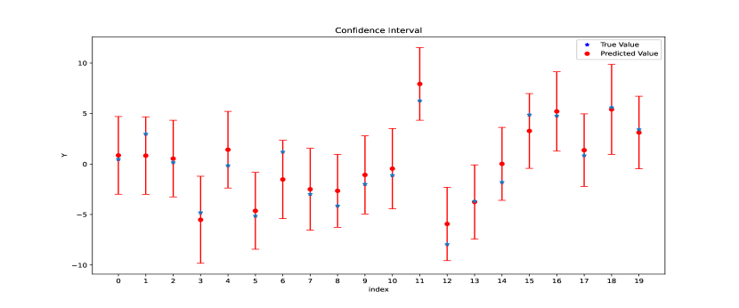
Figure 1: Prediction intervals of 20 testing points, where the y-axis is the response value, the x-axis is the index, and the blue point represents the true observation.

4.2 Real Data Example

As a different type of applications of the proposed method, we conducted unstructured network pruning experiments on CIFAR10 datasetKrizhevsky et al. (2009). Following the setup in Lin et al. (2020), we train the residual networkHe et al. (2016) with different networks size and pruned the network to different sparsity levels. The detailed experimental setup can be found in the supplementary material.

We compared the proposed methods, BNN_anneal (Algorithm 1) and BNN_average (averaged over last 75 networks simulated by the Bayesian version of the prior annealing algorithm), with several state-of-the-art unstructured pruning methods, including Consistent Sparse Deep Learning (BNN_BIC) Sun et al. (2021), Dynamic pruning with feedback (DPF) Lin et al. (2020), Dynamic Sparse Reparameterization (DSR) Mostafa and Wang (2019) and Sparse Momentum (SM) Dettmers and Zettlemoyer (2019). The results of the baseline methods were taken from Lin et al. (2020) and Sun et al. (2021). The results of prediction accuracy for different models and target sparsity levels were summarized in Table 2. Due to the threshold used in step (iii) of Algorithm 1, it is hard for our method to make the pruning ratio exactly the same as the targeted one. We intentionally make the pruning ratio smaller than the target ratio, while our method still achieve better test accuracy. Compared to BNN_BIC, the test accuracy is very close, but the result of BNN_BIC is obtained by running the experiment 10 times while our method only run once. To further demonstrate that the proposed method result in better model calibration, we followed the setup of Maddox et al. (2019) and compared the proposed method with DPF on several metrics designed for model calibration, including negtive log likelihood (NLL), symmetrized, discretized KL distance between in and out of sample entropy distributions (JS-Distance), and expected calibration error (ECE). For JS-Distance, we used the test data of SVHN data set as out-of-distribution samples. The results were summarized in Table 3. As discussed in Maddox et al. (2019); Guo et al. (2017), a well calibrated model tends to have smaller NLL, larger JS-Distance and smaller ECE. The comparison shows that the proposed method outperforms DPF in most cases. In addition to the network pruning method, we also train a dense model with the standard training set up. Compared to the dense model, the sparse network has worse accuracy, but it tends to outperform the dense network in terms of ECE and JS-Distance, which indicates that sparsification is also a useful way for improving calibration of the DNN.

Table 2: ResNet network pruning results for CIFAR-10 data, which were calculated by averaging over 3 independent runs with the standard deviation reported in the parentheses.

	ResNet-20			ResNet-32
Method	Pruning Ratio	Test Accuracy		Pruning Ratio	Test Accuracy
DNN_dense	100%	92.93(0.04)		100%	93.76(0.02)
BNN_average	19.85%(0.18%)	92.53(0.08)		9.99%(0.08%)	93.12(0.09)
BNN_anneal	19.80%(0.01%)	92.30(0.16)		9.97%(0.03%)	92.63(0.09)
BNN_BIC	19.67%(0.05%)	92.27(0.03)		9.53%(0.04%)	92.74(0.07)
SM	20%	91.54(0.16)		10%	91.54(0.18)
DSR	20%	91.78(0.28)		10%	91.41(0.23)
DPF	20%	92.17(0.21)		10%	92.42(0.18)
BNN_average	9.88%(0.02%)	91.65(0.08)		4.77%(0.08%)	91.30(0.16)
BNN_anneal	9.95%(0.03%)	91.28(0.11)		4.88%(0.02%)	91.17(0.08)
BNN_BIC	9.55%(0.03%)	91.27(0.05)		4.78%(0.01%)	91.21(0.01)
SM	10%	89.76(0.40)		5%	88.68(0.22)
DSR	10%	87.88(0.04)		5%	84.12(0.32)
DPF	10%	90.88(0.07)		5%	90.94(0.35)

Table 3: ResNet network pruning results for CIFAR-10 data, which were calculated by averaging over 3 independent runs with the standard deviation reported in the parentheses.

Method Model Pruning Ratio NLL JS-Distance ECE DNN_dense ResNet20 100% 0.2276(0.0021) 7.9118(0.9316) 0.02627(0.0005) BNN_average ResNet20 9.88%(0.02%) 0.2528(0.0029) 9.9641(0.3069) 0.0113(0.0010) BNN_anneal ResNet20 9.95%(0.03%) 0.2618(0.0037) 10.1251(0.1797) 0.0175(0.0011) DPF ResNet20 10% 0.2833(0.0004) 7.5712(0.4466) 0.0294(0.0009) BNN_average ResNet20 19.85%(0.18%) 0.2323(0.0033) 7.7007(0.5374) 0.0173(0.0014) BNN_anneal ResNet20 19.80%(0.01%) 0.2441(0.0042) 6.4435(0.2029) 0.0233(0.0020) DPF ResNet20 20% 0.2874(0.0029) 7.7329(0.1400) 0.0391(0.0001) DNN_dense ResNet32 100% 0.2042(0.0017) 6.7699(0.5253) 0.02613(0.00029) BNN_average ResNet32 9.99%(0.08%) 0.2116(0.0012) 9.4549(0.5456) 0.0132(0.0001) BNN_anneal ResNet32 9.97%(0.03%) 0.2218(0.0013) 8.5447(0.1393) 0.0192(0.0009) DPF ResNet32 10% 0.2677(0.0041) 7.8693(0.1840) 0.0364(0.0015) BNN_average ResNet32 4.77%(0.08%) 0.2587(0.0022) 7.0117(0.2222) 0.0100(0.0002) BNN_anneal ResNet32 4.88%(0.02%) 0.2676(0.0014) 6.8440(0.4850) 0.0149(0.0006) DPF ResNet32 5% 0.2921(0.0067) 6.3990(0.8384) 0.0276(0.0019)

5 Conclusion

This work, together with Sun et al. (2021), has built a solid theoretical foundation for sparse deep learning, which has successfully tamed the sparse deep neural network into the framework of statistical modeling. As implied by Lemma 2.1, Lemma 2.2, Theorem 2.1, and Theorem 2.2, the sparse DNN can be simply viewed as a nonlinear statistical model which, like a traditional statistical model, possesses many nice properties such as posterior consistency, variable selection consistency, and asymptotic normality. We have shown how the prediction uncertainty of the sparse DNN can be quantified based on the asymptotic normality theory, and provided algorithms for training sparse DNNs with theoretical guarantees for its convergence to the global optimum. The latter ensures the validity of the down-stream statistical inference.

Appendix A Supplementary material of "Sparse Deep Learning: A New Framework Immune to Local Traps and Miscalibration"

A.1 Proof of Theorem 2.1

Proof.

We first define the equivalent class of neural network parameters. Given a parameter vector ${\boldsymbol{\beta}}$ and the corresponding structure parameter vector ${\boldsymbol{\gamma}}$, its equivalent class is given by

$$Q_{E}({\boldsymbol{\beta}},{\boldsymbol{\gamma}})=\{(\tilde{{\boldsymbol{\beta}}},\tilde{{\boldsymbol{\gamma}}}):\nu_{g}(\tilde{{\boldsymbol{\beta}}},\tilde{{\boldsymbol{\gamma}}})=({\boldsymbol{\beta}},{\boldsymbol{\gamma}}),\mu(\tilde{{\boldsymbol{\beta}}},\tilde{{\boldsymbol{\gamma}}},{\boldsymbol{x}})=\mu({\boldsymbol{\beta}},{\boldsymbol{\gamma}},{\boldsymbol{x}}),\forall{\boldsymbol{x}}\},$$

where $\nu_{g}(\cdot)$ denotes a generic mapping that contains only the transformations of node permutation and weight sign flipping. Specifically, we define

$$Q_{E}^{*}=Q_{E}({\boldsymbol{\beta}}^{*},{\boldsymbol{\gamma}}^{*}),$$

which represents the equivalent class of true DNN model.

Let $B_{\delta_{n}}({\boldsymbol{\beta}}^{*})=\{{\boldsymbol{\beta}}:|{\boldsymbol{\beta}}_{i}-{\boldsymbol{\beta}}^{*}_{i}|<\delta_{n},\forall i\in{\boldsymbol{\gamma}}^{*},|{\boldsymbol{\beta}}_{i}-{\boldsymbol{\beta}}^{*}_{i}|<2\sigma_{0,n}\log(\frac{\sigma_{1,n}}{\lambda_{n}\sigma_{0,n}}),\forall i\notin{\boldsymbol{\gamma}}^{*}\}$. By assumption C.1, ${\boldsymbol{\beta}}^{*}$ is generic (i.e. $Q_{E}({\boldsymbol{\beta}}^{*})$ contains only reparameterizations of weight sign-flipping or node permutations as defined in Feng and Simon [2017] and Fefferman [1994]) and $\min_{i\in{\boldsymbol{\gamma}}^{*}}|{\boldsymbol{\beta}}^{*}_{i}|-\delta_{n}>(C-1)\delta_{n}>\delta_{n}$, then for any ${\boldsymbol{\beta}}^{*(1)},{\boldsymbol{\beta}}^{*(2)}\in Q_{E}^{*}$, $B_{\delta_{n}}({\boldsymbol{\beta}}^{*(1)})\cap B_{\delta_{n}}({\boldsymbol{\beta}}^{*(2)})=\emptyset$, and thus $\{{\boldsymbol{\beta}}:\tilde{\nu}({\boldsymbol{\beta}})\in B_{\delta_{n}}({\boldsymbol{\beta}}^{*})\}=\cup_{{\boldsymbol{\beta}}\in Q_{E}^{*}}B_{\delta_{n}}({\boldsymbol{\beta}})$. In what follows, we will first show $\pi(\cup_{{\boldsymbol{\beta}}\in Q_{E}^{*}}B_{\delta_{n}}({\boldsymbol{\beta}})\mid D_{n})\rightarrow 1$ as $n\to\infty$, which means the most posterior mass falls in the neighbourhood of true parameter.

Remark on the notation: $\tilde{\nu}(\cdot)$ is similar to $\nu(\cdot)$ defined in Section 2.1 of the main text. They both map the set $Q_{E}({\boldsymbol{\beta}},{\boldsymbol{\gamma}})$ to a unique network. The difference between them is that $\|\nu({\boldsymbol{\beta}})-{\boldsymbol{\beta}}^{*}\|_{\infty}$ may be arbitrary, but $\|\tilde{\nu}({\boldsymbol{\beta}})-{\boldsymbol{\beta}}^{*}\|_{\infty}$ is minimized. In other words, $\nu({\boldsymbol{\beta}},{\boldsymbol{\gamma}})$ is to find an arbitrary network in $Q_{E}({\boldsymbol{\beta}},{\boldsymbol{\gamma}})$ as the representative of the equivalent class, while $\tilde{\nu}({\boldsymbol{\beta}},{\boldsymbol{\gamma}})$ is to find a representative in $Q_{E}({\boldsymbol{\beta}},{\boldsymbol{\gamma}})$ such that the distance between ${\boldsymbol{\beta}}^{*}$ and the representative is minimized. In what follows, we will use $\tilde{\nu}({\boldsymbol{\beta}})$ and $\tilde{\nu}({\boldsymbol{\gamma}})$ to denote the connection weight and network structure of $\tilde{\nu}({\boldsymbol{\beta}},{\boldsymbol{\gamma}})$, respectively. With a slight abuse of notation, we will use $\tilde{\nu}({\boldsymbol{\beta}})_{i}$ to denote the $i$th component of $\tilde{\nu}({\boldsymbol{\beta}})$, and use $\tilde{\nu}({\boldsymbol{\gamma}})_{i}$ to denote the $i$th component of $\tilde{\nu}({\boldsymbol{\gamma}})$.

Recall that the marginal posterior inclusion probability is given by

$$q_{i}=\int\sum_{{\boldsymbol{\gamma}}}e_{i|\tilde{\nu}({\boldsymbol{\beta}},{\boldsymbol{\gamma}})}\pi({\boldsymbol{\gamma}}|{\boldsymbol{\beta}},D_{n})\pi({\boldsymbol{\beta}}|D_{n})d{\boldsymbol{\beta}}=\int\pi(\tilde{\nu}({\boldsymbol{\gamma}})_{i}=1|{\boldsymbol{\beta}})\pi({\boldsymbol{\beta}}|D_{n})d{\boldsymbol{\beta}}.$$

For the mixture Gaussian prior,

$$\pi({\boldsymbol{\gamma}}_{i}=1|{\boldsymbol{\beta}})=\frac{1}{1+\frac{\sigma_{1,n}(1-\lambda_{n})}{\sigma_{0,n}\lambda_{n}}e^{-(\frac{1}{2\sigma_{0,n}^{2}}-\frac{1}{2\sigma_{1,n}^{2}}){\boldsymbol{\beta}}_{i}^{2}}},$$

which increases with respect to $|{\boldsymbol{\beta}}_{i}|$. In particular, if $|{\boldsymbol{\beta}}_{i}|>2\sigma_{0,n}\log(\frac{\sigma_{1,n}}{\lambda_{n}\sigma_{0,n}})$, then $\pi({\boldsymbol{\gamma}}_{i}=1|{\boldsymbol{\beta}})>\frac{1}{2}$.

For the mixture Gaussian prior,

$$\begin{split}&\pi({\boldsymbol{\beta}}\notin\cup_{{\boldsymbol{\beta}}\in Q_{E}^{*}}B_{\delta_{n}}({\boldsymbol{\beta}})\mid D_{n})\\ \leq&\pi(\exists i\notin{\boldsymbol{\gamma}}^{*},|\tilde{\nu}({\boldsymbol{\beta}})_{i}|>2\sigma_{0,n}\log(\frac{\sigma_{1,n}}{\lambda_{n}\sigma_{0,n}})\mid D_{n})+\pi(\exists i\in{\boldsymbol{\gamma}}^{*},|\tilde{\nu}({\boldsymbol{\beta}})_{i}-{\boldsymbol{\beta}}^{*}_{i}|>\delta_{n}\mid D_{n}).\end{split}$$

For the first term, note that for a given $i\notin{\boldsymbol{\gamma}}^{*}$,

$$\begin{split}\pi(|\tilde{\nu}({\boldsymbol{\beta}})_{i}|>2\sigma_{0,n}\log(\frac{\sigma_{1,n}}{\lambda_{n}\sigma_{0,n}})\mid D_{n})\leq&\pi(\pi(\tilde{\nu}({\boldsymbol{\gamma}})_{i}=1|{\boldsymbol{\beta}})>\frac{1}{2}\mid D_{n})\\ \leq&2\int\pi(\tilde{\nu}({\boldsymbol{\gamma}})_{i}=1|{\boldsymbol{\beta}})\pi({\boldsymbol{\beta}}|D_{n})d{\boldsymbol{\beta}}\\ \leq&2\rho(\epsilon_{n})+2\pi(d(p_{\boldsymbol{\beta}},p_{\mu^{*}})\geq\epsilon_{n}\mid D_{n})\rightarrow 0.\end{split}$$

Then we have

$$\begin{split}\pi(\exists i\notin{\boldsymbol{\gamma}}^{*},|\tilde{\nu}({\boldsymbol{\beta}})_{i}|>2\sigma_{0,n}\log(\frac{\sigma_{1,n}}{\lambda_{n}\sigma_{0,n}})\mid D_{n})=&\pi(\max_{i\notin{\boldsymbol{\gamma}}^{*}}|\tilde{\nu}({\boldsymbol{\beta}})_{i}|>2\sigma_{0,n}\log(\frac{\sigma_{1,n}}{\lambda_{n}\sigma_{0,n}})\mid D_{n})\\ \leq&\pi(\max_{i\notin{\boldsymbol{\gamma}}^{*}}\pi(\tilde{\nu}({\boldsymbol{\gamma}})_{i}=1|{\boldsymbol{\beta}})>\frac{1}{2}\mid D_{n})\\ \leq&\sum_{i\notin{\boldsymbol{\gamma}}^{*}}\pi(\pi(\tilde{\nu}({\boldsymbol{\gamma}})_{i}=1|{\boldsymbol{\beta}})>\frac{1}{2}\mid D_{n})\\ \leq&2K_{n}\rho(\epsilon_{n})+2K_{n}\pi(d(p_{\boldsymbol{\beta}},p_{\mu^{*}})\geq\epsilon_{n}\mid D_{n})\rightarrow 0.\end{split}$$

For the second term, by condition C.1 and Lemma 2.1,

$$\begin{split}&\pi(\exists i\in{\boldsymbol{\gamma}}^{*},|\tilde{\nu}({\boldsymbol{\beta}})_{i}-{\boldsymbol{\beta}}^{*}_{i}|>\delta_{n}\mid D_{n})=\pi(\max_{i\in{\boldsymbol{\gamma}}^{*}}|\tilde{\nu}({\boldsymbol{\beta}})_{i}-{\boldsymbol{\beta}}^{*}_{i}|>\delta_{n}\mid D_{n})\\ =&\pi(\max_{i\in{\boldsymbol{\gamma}}^{*}}|\tilde{\nu}({\boldsymbol{\beta}})_{i}-{\boldsymbol{\beta}}^{*}_{i}|>\delta_{n},d(p_{\boldsymbol{\beta}},p_{\mu^{*}})\leq\epsilon_{n}\mid D_{n})\\ &+\pi(\max_{i\in{\boldsymbol{\gamma}}^{*}}|\tilde{\nu}({\boldsymbol{\beta}})_{i}-{\boldsymbol{\beta}}^{*}_{i}|>\delta_{n},d(p_{\boldsymbol{\beta}},p_{\mu^{*}})\geq\epsilon_{n}\mid D_{n})\\ \leq&\pi(A(\epsilon_{n},\delta_{n})\mid D_{n})+\pi(d(p_{\boldsymbol{\beta}},p_{\mu^{*}})\geq\epsilon_{n}\mid D_{n})\rightarrow 0.\end{split}$$

Summarizing the above two terms, we have $\pi(\cup_{{\boldsymbol{\beta}}\in Q_{E}^{*}}B_{\delta_{n}}({\boldsymbol{\beta}})\mid D_{n})\rightarrow 1$.

Let $Q_{n}=|Q_{E}^{*}|$ be the number of equivalent true DNN model. By the generic assumption of ${\boldsymbol{\beta}}^{*}$, for any ${\boldsymbol{\beta}}^{*(1)},{\boldsymbol{\beta}}^{*(2)}\in Q_{E}^{*}$, $B_{\delta_{n}}({\boldsymbol{\beta}}^{*(1)})\cap B_{\delta_{n}}({\boldsymbol{\beta}}^{*(2)})=\emptyset$. Then in $B_{\delta_{n}}({\boldsymbol{\beta}}^{*})$, the posterior density of $\tilde{\nu}({\boldsymbol{\beta}})$ is $Q_{n}$ times the posterior density of ${\boldsymbol{\beta}}$. Then for a function $f(\cdot)$ of $\tilde{\nu}({\boldsymbol{\beta}})$, by changing variable,

$$\int_{\tilde{\nu}({\boldsymbol{\beta}})\in B_{\delta_{n}}({\boldsymbol{\beta}}^{*})}f(\tilde{\nu}({\boldsymbol{\beta}}))\pi(\tilde{\nu}({\boldsymbol{\beta}})|D_{n})d\tilde{\nu}({\boldsymbol{\beta}})=Q_{n}\int_{B_{\delta_{n}}({\boldsymbol{\beta}}^{*})}f({\boldsymbol{\beta}})\pi({\boldsymbol{\beta}}|D_{n})d{\boldsymbol{\beta}}.$$

Thus, we only need to consider the integration on $B_{\delta_{n}}({\boldsymbol{\beta}}^{*})$. Define

$$\hat{{\boldsymbol{\beta}}}_{i}=\begin{cases}{\boldsymbol{\beta}}^{*}_{i}-\sum_{j\in{\boldsymbol{\gamma}}^{*}}h^{i,j}({\boldsymbol{\beta}}^{*})h_{j}({\boldsymbol{\beta}}^{*}),&\forall i\in{\boldsymbol{\gamma}}^{*},\\ 0,&\forall i\not\in{\boldsymbol{\gamma}}^{*}.\\ \end{cases}$$

We will first prove that for any real vector ${\boldsymbol{t}}$,

$$\begin{split}E(e^{\sqrt{n}{\boldsymbol{t}}^{T}(\tilde{\nu}({\boldsymbol{\beta}})-\hat{{\boldsymbol{\beta}}})}\mid D_{n},B_{\delta_{n}}({\boldsymbol{\beta}}^{*})):=&\frac{\int_{B_{\delta_{n}}({\boldsymbol{\beta}}^{*})}e^{\sqrt{n}{\boldsymbol{t}}^{T}(\tilde{\nu}({\boldsymbol{\beta}})-\hat{{\boldsymbol{\beta}}})}\pi(\tilde{\nu}({\boldsymbol{\beta}})|D_{n})d\tilde{\nu}({\boldsymbol{\beta}})}{\int_{B_{\delta_{n}}({\boldsymbol{\beta}}^{*})}\pi(\tilde{\nu}({\boldsymbol{\beta}})|D_{n})d\tilde{\nu}({\boldsymbol{\beta}})}\\ =&\frac{\int_{B_{\delta_{n}}({\boldsymbol{\beta}}^{*})}e^{\sqrt{n}{\boldsymbol{t}}^{T}({\boldsymbol{\beta}}-\hat{{\boldsymbol{\beta}}})}e^{nl_{n}({\boldsymbol{\beta}})}\pi({\boldsymbol{\beta}})d{\boldsymbol{\beta}}}{\int_{B_{\delta_{n}}({\boldsymbol{\beta}}^{*})}e^{nl_{n}({\boldsymbol{\beta}})}\pi({\boldsymbol{\beta}})d{\boldsymbol{\beta}}}\\ =&e^{\frac{1}{2}{\boldsymbol{t}}^{T}{\boldsymbol{V}}{\boldsymbol{t}}+o_{P^{*}}(1)}.\end{split}$$ (6)

For any ${\boldsymbol{\beta}}\in B_{\delta_{n}}({\boldsymbol{\beta}}^{*})$, we have

$$\begin{split}|\sqrt{n}({\boldsymbol{t}}^{T}({\boldsymbol{\beta}}-{\boldsymbol{\beta}}_{{\boldsymbol{\gamma}}^{*}}))|\leq\sqrt{n}K_{n}||{\boldsymbol{t}}||_{\infty}2\sigma_{0,n}\log(\frac{\sigma_{1,n}}{\lambda_{n}\sigma_{0,n}})=o(1),\end{split}$$

$$\begin{split}|n(l_{n}({\boldsymbol{\beta}})-l_{n}({\boldsymbol{\beta}}_{{\boldsymbol{\gamma}}^{*}}))|=|n\sum_{i\notin{\boldsymbol{\gamma}}^{*}}{\boldsymbol{\beta}}_{i}(h_{i}(\tilde{{\boldsymbol{\beta}}}))|\leq nK_{n}M2\sigma_{0,n}\log(\frac{\sigma_{1,n}}{\lambda_{n}\sigma_{0,n}})=o(1).\end{split}$$

Then, we have

$$\begin{split}\sqrt{n}{\boldsymbol{t}}^{T}({\boldsymbol{\beta}}-\hat{{\boldsymbol{\beta}}})=&\sqrt{n}{\boldsymbol{t}}^{T}({\boldsymbol{\beta}}-{\boldsymbol{\beta}}_{{\boldsymbol{\gamma}}^{*}}+{\boldsymbol{\beta}}_{{\boldsymbol{\gamma}}^{*}}-{\boldsymbol{\beta}}^{*})+\sqrt{n}\sum_{i,j\in{\boldsymbol{\gamma}}^{*}}h^{i,j}({\boldsymbol{\beta}}^{*}){\boldsymbol{t}}_{j}h_{i}({\boldsymbol{\beta}}^{*}))\\ =&o(1)+\sqrt{n}\sum_{i\in{\boldsymbol{\gamma}}^{*}}({\boldsymbol{\beta}}_{i}-{\boldsymbol{\beta}}^{*}_{i}){\boldsymbol{t}}_{i}+\sqrt{n}\sum_{i,j\in{\boldsymbol{\gamma}}^{*}}h^{i,j}({\boldsymbol{\beta}}^{*}){\boldsymbol{t}}_{j}h_{i}({\boldsymbol{\beta}}^{*}),\end{split}$$ (7)

$$\begin{split}nl_{n}({\boldsymbol{\beta}})-nl_{n}({\boldsymbol{\beta}}^{*})=&n(l_{n}({\boldsymbol{\beta}})-l_{n}({\boldsymbol{\beta}}_{{\boldsymbol{\gamma}}^{*}})+l_{n}({\boldsymbol{\beta}}_{{\boldsymbol{\gamma}}^{*}})-nl_{n}({\boldsymbol{\beta}}^{*}))\\ =&o(1)+n\sum_{i\in{\boldsymbol{\gamma}}^{*}}({\boldsymbol{\beta}}_{i}-{\boldsymbol{\beta}}^{*}_{i})h_{i}({\boldsymbol{\beta}}^{*})+\frac{n}{2}\sum_{i,j\in{\boldsymbol{\gamma}}^{*}}h_{i,j}({\boldsymbol{\beta}}^{*})({\boldsymbol{\beta}}_{i}-{\boldsymbol{\beta}}_{i}^{*})({\boldsymbol{\beta}}_{j}-{\boldsymbol{\beta}}^{*}_{j})\\ &+\frac{n}{6}\sum_{i,j,k\in{\boldsymbol{\gamma}}^{*}}h_{i,j,k}(\check{{\boldsymbol{\beta}}})({\boldsymbol{\beta}}_{i}-{\boldsymbol{\beta}}_{i}^{*})({\boldsymbol{\beta}}_{j}-{\boldsymbol{\beta}}^{*}_{j})({\boldsymbol{\beta}}_{k}-{\boldsymbol{\beta}}^{*}_{k}),\end{split}$$ (8)

where $\check{{\boldsymbol{\beta}}}$ is a point between ${\boldsymbol{\beta}}_{{\boldsymbol{\gamma}}^{*}}$ and ${\boldsymbol{\beta}}^{*}$. Note that for ${\boldsymbol{\beta}}\in B_{\delta_{n}}({\boldsymbol{\beta}}^{*})$, $|{\boldsymbol{\beta}}_{i}-{\boldsymbol{\beta}}^{*}_{i}|\leq\delta_{n}\lesssim\frac{1}{\sqrt[3]{n}r_{n}}$, we have $\frac{n}{6}\sum_{i,j,k\in{\boldsymbol{\gamma}}^{*}}h_{i,j,k}(\check{{\boldsymbol{\beta}}})({\boldsymbol{\beta}}_{i}-{\boldsymbol{\beta}}_{i}^{*})({\boldsymbol{\beta}}_{j}-{\boldsymbol{\beta}}^{*}_{j})({\boldsymbol{\beta}}_{k}-{\boldsymbol{\beta}}^{*}_{k})=o(1)$.

Let ${\boldsymbol{\beta}}^{(t)}$ be network parameters satisfying ${\boldsymbol{\beta}}^{(t)}_{i}={\boldsymbol{\beta}}_{i}+\frac{1}{\sqrt{n}}\sum_{j\in{\boldsymbol{\gamma}}^{*}}h^{i,j}({\boldsymbol{\beta}}^{*}){\boldsymbol{t}}_{j},\forall i\in{\boldsymbol{\gamma}}^{*}$ and ${\boldsymbol{\beta}}^{(t)}_{i}={\boldsymbol{\beta}}_{i},\forall i\notin{\boldsymbol{\gamma}}^{*}$. Note that $\frac{1}{\sqrt{n}}\sum_{j\in{\boldsymbol{\gamma}}^{*}}h^{i,j}({\boldsymbol{\beta}}^{*}){\boldsymbol{t}}_{j}\leq\frac{r_{n}||{\boldsymbol{t}}||_{\infty}M}{\sqrt{n}}\lesssim\delta_{n}$, for large enough $n$, $|{\boldsymbol{\beta}}^{(t)}_{i}|<2\delta_{n}$ $\forall i\in{\boldsymbol{\gamma}}^{*}$. Thus, we have

$$\begin{split}nl_{n}({\boldsymbol{\beta}}^{(t)})-nl_{n}({\boldsymbol{\beta}}^{*})=&n(l_{n}({\boldsymbol{\beta}}^{(t)})-l_{n}({\boldsymbol{\beta}}^{(t)}_{{\boldsymbol{\gamma}}^{*}})+l_{n}({\boldsymbol{\beta}}^{(t)}_{{\boldsymbol{\gamma}}^{*}})-nl_{n}({\boldsymbol{\beta}}^{*}))\\ =&o(1)+n\sum_{i\in{\boldsymbol{\gamma}}^{*}}({\boldsymbol{\beta}}^{(t)}_{i}-{\boldsymbol{\beta}}^{*}_{i})h_{i}({\boldsymbol{\beta}}^{*})+\frac{n}{2}\sum_{i,j\in{\boldsymbol{\gamma}}^{*}}h_{i,j}({\boldsymbol{\beta}}^{*})({\boldsymbol{\beta}}^{(t)}_{i}-{\boldsymbol{\beta}}_{i}^{*})({\boldsymbol{\beta}}^{(t)}_{j}-{\boldsymbol{\beta}}^{*}_{j})\\ =&o(1)+n\sum_{i\in{\boldsymbol{\gamma}}^{*}}({\boldsymbol{\beta}}_{i}-{\boldsymbol{\beta}}^{*}_{i})h_{i}({\boldsymbol{\beta}}^{*})+\frac{n}{2}\sum_{i,j\in{\boldsymbol{\gamma}}^{*}}h_{i,j}({\boldsymbol{\beta}}^{*})({\boldsymbol{\beta}}_{i}-{\boldsymbol{\beta}}_{i}^{*})({\boldsymbol{\beta}}_{j}-{\boldsymbol{\beta}}^{*}_{j})\\ &+\sqrt{n}\sum_{i,j\in{\boldsymbol{\gamma}}^{*}}h^{i,j}({\boldsymbol{\beta}}^{*}){\boldsymbol{t}}_{j}h_{i}({\boldsymbol{\beta}}^{*})+\sqrt{n}\sum_{i\in{\boldsymbol{\gamma}}^{*}}({\boldsymbol{\beta}}_{i}-{\boldsymbol{\beta}}^{*}_{i}){\boldsymbol{t}}_{i}+\frac{1}{2}\sum_{i,j\in{\boldsymbol{\gamma}}^{*}}h^{i,j}({\boldsymbol{\beta}}^{*}){\boldsymbol{t}}_{i}{\boldsymbol{t}}_{j}\\ =&o(1)+\sqrt{n}{\boldsymbol{t}}^{T}({\boldsymbol{\beta}}-\hat{{\boldsymbol{\beta}}})+nl_{n}({\boldsymbol{\beta}})-nl_{n}({\boldsymbol{\beta}}^{*})+\frac{1}{2}\sum_{i,j\in{\boldsymbol{\gamma}}^{*}}h^{i,j}({\boldsymbol{\beta}}^{*}){\boldsymbol{t}}_{i}{\boldsymbol{t}}_{j},\end{split}$$ (9)

where the last equality is derived by replacing appropriate terms by $\sqrt{n}{\boldsymbol{t}}^{T}({\boldsymbol{\beta}}-\hat{{\boldsymbol{\beta}}})$ and $nl_{n}({\boldsymbol{\beta}})-nl_{n}({\boldsymbol{\beta}}^{*})$ based on (7) and (8), respectively; and the third equality is derived based on the following calculation:

$$\begin{split}&\frac{n}{2}\sum_{i,j\in{\boldsymbol{\gamma}}^{*}}h_{i,j}({\boldsymbol{\beta}}^{*})({\boldsymbol{\beta}}^{(t)}_{i}-{\boldsymbol{\beta}}_{i}^{*})({\boldsymbol{\beta}}^{(t)}_{j}-{\boldsymbol{\beta}}^{*}_{j})\\ =&\frac{n}{2}\sum_{i,j\in{\boldsymbol{\gamma}}^{*}}h_{i,j}({\boldsymbol{\beta}}^{*})({\boldsymbol{\beta}}_{i}-{\boldsymbol{\beta}}_{i}^{*}+\frac{1}{\sqrt{n}}\sum_{k\in{\boldsymbol{\gamma}}^{*}}h^{i,k}({\boldsymbol{\beta}}^{*}){\boldsymbol{t}}_{k})({\boldsymbol{\beta}}_{j}-{\boldsymbol{\beta}}_{j}^{*}+\frac{1}{\sqrt{n}}\sum_{k\in{\boldsymbol{\gamma}}^{*}}h^{j,k}({\boldsymbol{\beta}}^{*}){\boldsymbol{t}}_{k})\\ =&\frac{n}{2}\sum_{i,j\in{\boldsymbol{\gamma}}^{*}}h_{i,j}({\boldsymbol{\beta}}^{*})({\boldsymbol{\beta}}_{i}-{\boldsymbol{\beta}}_{i}^{*})({\boldsymbol{\beta}}_{j}-{\boldsymbol{\beta}}_{j}^{*})+2\times\frac{n}{2}\sum_{i,j\in{\boldsymbol{\gamma}}^{*}}h_{i,j}({\boldsymbol{\beta}}^{*})\frac{1}{\sqrt{n}}\sum_{k\in{\boldsymbol{\gamma}}^{*}}h^{i,k}({\boldsymbol{\beta}}^{*}){\boldsymbol{t}}_{k}({\boldsymbol{\beta}}_{j}-{\boldsymbol{\beta}}_{j}^{*})\\ &+\frac{n}{2}\sum_{i,j\in{\boldsymbol{\gamma}}^{*}}h_{i,j}({\boldsymbol{\beta}}^{*})(\frac{1}{\sqrt{n}}\sum_{k\in{\boldsymbol{\gamma}}^{*}}h^{i,k}({\boldsymbol{\beta}}^{*}){\boldsymbol{t}}_{k})(\frac{1}{\sqrt{n}}\sum_{k\in{\boldsymbol{\gamma}}^{*}}h^{j,k}({\boldsymbol{\beta}}^{*}){\boldsymbol{t}}_{k})\\ =&\frac{n}{2}\sum_{i,j\in{\boldsymbol{\gamma}}^{*}}h_{i,j}({\boldsymbol{\beta}}^{*})({\boldsymbol{\beta}}_{i}-{\boldsymbol{\beta}}_{i}^{*})({\boldsymbol{\beta}}_{j}-{\boldsymbol{\beta}}_{j}^{*})+\sqrt{n}\sum_{i\in{\boldsymbol{\gamma}}^{*}}({\boldsymbol{\beta}}_{i}-{\boldsymbol{\beta}}^{*}_{i}){\boldsymbol{t}}_{i}+\frac{1}{2}\sum_{i,j\in{\boldsymbol{\gamma}}^{*}}h^{i,j}({\boldsymbol{\beta}}^{*}){\boldsymbol{t}}_{i}{\boldsymbol{t}}_{j},\\ \end{split}$$ (10)

where the second and third terms in the last equality are derived based on the relation $\sum_{i\in{\boldsymbol{\gamma}}^{*}}h_{i,j}({\boldsymbol{\beta}}^{*})h^{i,k}({\boldsymbol{\beta}}^{*})=\delta_{j,k}$, where $\delta_{j,k}=1$ if $j=k$, $\delta_{j,k}=0$ if $j\neq k$.

By rearranging the terms in (9), we have

$$\begin{split}&\int_{B_{\delta_{n}}({\boldsymbol{\beta}}^{*})}\exp\{\sqrt{n}{\boldsymbol{t}}^{T}({\boldsymbol{\beta}}-\hat{{\boldsymbol{\beta}}})+nl_{n}({\boldsymbol{\beta}})\}\pi({\boldsymbol{\beta}})d{\boldsymbol{\beta}}\\ &=\exp\left\{-\frac{1}{2}\sum_{i,j\in{\boldsymbol{\gamma}}^{*}}h^{i,j}({\boldsymbol{\beta}}^{*}){\boldsymbol{t}}_{i}{\boldsymbol{t}}_{j}+o(1)\right\}\int_{B_{\delta_{n}}({\boldsymbol{\beta}}^{*})}e^{nl_{n}({\boldsymbol{\beta}}^{(t)})}\pi({\boldsymbol{\beta}})d{\boldsymbol{\beta}}.\end{split}$$

For ${\boldsymbol{\beta}}\in B_{\delta_{n}}({\boldsymbol{\beta}}^{*}),i\in{\boldsymbol{\gamma}}^{*}$, by Assumption C.1, there exists a constant $C>2$ such that

$$\begin{split}|{\boldsymbol{\beta}}^{(t)}_{i}|&\geq|{\boldsymbol{\beta}}_{i}|-\frac{r_{n}||{\boldsymbol{t}}||_{\infty}M}{\sqrt{n}}\geq|{\boldsymbol{\beta}}^{*}_{i}|-2\delta_{n}\geq(C-2)\delta_{n}\gtrsim\frac{r_{n}}{\sqrt{n}}\\ &\gtrsim\sqrt{\left(\frac{1}{2\sigma_{0,n}^{2}}-\frac{1}{2\sigma_{1,n}^{2}}\right)^{-1}\log\left(\frac{r_{n}(1-\lambda_{n})\sigma_{1,n}}{\sigma_{0,n}\lambda_{n}}\right)}.\end{split}$$

Then we have

$$\frac{\sigma_{1,n}(1-\lambda_{n})}{\sigma_{0,n}\lambda_{n}}e^{-(\frac{1}{2\sigma_{0,n}^{2}}-\frac{1}{2\sigma_{1,n}^{2}})({\boldsymbol{\beta}}^{(t)}_{i})^{2}}\lesssim\frac{1}{r_{n}}.$$

It is easy to see that the above formula also holds if we replace ${\boldsymbol{\beta}}^{(t)}_{i}$ by ${\boldsymbol{\beta}}_{i}$. Note that the mixture Gaussian prior of ${\boldsymbol{\beta}}_{i}$ can be written as

$$\pi({\boldsymbol{\beta}}_{i})=\frac{\lambda_{n}}{\sqrt{2\pi}\sigma_{1,n}}e^{-\frac{{\boldsymbol{\beta}}_{i}^{2}}{2\sigma_{1,n}^{2}}}\left(1+\frac{\sigma_{1,n}(1-\lambda_{n})}{\sigma_{0,n}\lambda_{n}}e^{-(\frac{1}{2\sigma_{0,n}^{2}}-\frac{1}{2\sigma_{1,n}^{2}}){\boldsymbol{\beta}}_{i}^{2}}\right).$$

Since $|{\boldsymbol{\beta}}_{i}-{\boldsymbol{\beta}}^{(t)}_{i}|\lesssim\delta_{n}\lesssim\frac{1}{\sqrt[3]{n}r_{n}}$, $|{\boldsymbol{\beta}}_{i}+{\boldsymbol{\beta}}^{(t)}_{i}|<2E_{n}+3\delta_{n}\lesssim E_{n}$, and $\frac{1}{\sigma_{1,n}^{2}}\lesssim\frac{H_{n}\log(n)+\log(\bar{L})}{E_{n}^{2}}$, we have

$$\frac{r_{n}}{\sigma_{1,n}^{2}}({\boldsymbol{\beta}}_{i}-{\boldsymbol{\beta}}^{(t)}_{i})({\boldsymbol{\beta}}_{i}+{\boldsymbol{\beta}}^{(t)}_{i})=\frac{H_{n}\log(n)+\log(\bar{L})}{n^{C_{1}+1/3}}=o(1),$$

by the condition $C_{1}>2/3$ and $H_{n}\log(n)+\log(\bar{L})\prec n^{1-\epsilon}$. Thus, $\frac{\pi({\boldsymbol{\beta}})}{\pi({\boldsymbol{\beta}}^{(t)})}=\prod_{i\in{\boldsymbol{\gamma}}^{*}}\frac{\pi({\boldsymbol{\beta}}_{i})}{\pi({\boldsymbol{\beta}}^{(t)}_{i})}=1+o(1)$, and

$$\begin{split}\int_{B_{\delta_{n}}({\boldsymbol{\beta}}^{*})}e^{nl_{n}({\boldsymbol{\beta}}^{(t)})}\pi({\boldsymbol{\beta}})d{\boldsymbol{\beta}}=&(1+o(1))\int_{{\boldsymbol{\beta}}^{(t)}\in B_{\delta_{n}}({\boldsymbol{\beta}}^{*})}e^{nl_{n}({\boldsymbol{\beta}}^{(t)})}\pi({\boldsymbol{\beta}}^{(t)})d{\boldsymbol{\beta}}^{(t)}\\ =&(1+o(1))C_{N}\pi({\boldsymbol{\beta}}^{(t)}\in B_{\delta_{n}}({\boldsymbol{\beta}}^{*})\mid D_{n}),\end{split}$$ (11)

where $C_{N}$ is the normalizing constant of the posterior. Note that $||{\boldsymbol{\beta}}^{(t)}-{\boldsymbol{\beta}}||_{\infty}\lesssim\delta_{n}$, we have $\pi({\boldsymbol{\beta}}^{(t)}\in B_{\delta_{n}}({\boldsymbol{\beta}}^{*})\mid D_{n})\rightarrow\pi({\boldsymbol{\beta}}\in B_{\delta_{n}}({\boldsymbol{\beta}}^{*})\mid D_{n})$. Moreover, since $-\frac{1}{2}\sum_{i,j\in{\boldsymbol{\gamma}}^{*}}h^{i,j}({\boldsymbol{\beta}}^{*}){\boldsymbol{t}}_{i}{\boldsymbol{t}}_{j}\rightarrow\frac{1}{2}{\boldsymbol{t}}^{T}{\boldsymbol{V}}{\boldsymbol{t}}$, we have

$$E(e^{\sqrt{n}{\boldsymbol{t}}^{T}(\tilde{\nu}({\boldsymbol{\beta}})-\hat{{\boldsymbol{\beta}}})}\mid D_{n},B_{\delta_{n}}({\boldsymbol{\beta}}^{*}))=\frac{\int_{B_{\delta_{n}}({\boldsymbol{\beta}}^{*})}e^{\sqrt{n}{\boldsymbol{t}}^{T}({\boldsymbol{\beta}}-\hat{{\boldsymbol{\beta}}})}e^{nh_{n}({\boldsymbol{\beta}})}\pi({\boldsymbol{\beta}})d{\boldsymbol{\beta}}}{\int_{B_{\delta_{n}}({\boldsymbol{\beta}}^{*})}e^{nh_{n}({\boldsymbol{\beta}})}\pi({\boldsymbol{\beta}})d{\boldsymbol{\beta}}}=e^{\frac{{\boldsymbol{t}}^{T}{\boldsymbol{V}}{\boldsymbol{t}}}{2}+o_{P^{*}}(1)}.$$

Combining the above result with the fact that $\pi(\tilde{\nu}({\boldsymbol{\beta}})\in B_{\delta_{n}}({\boldsymbol{\beta}}^{*})\mid D_{n})\rightarrow 1$, by section 1 of Castillo and Rousseau [2015], we have

$$\pi[\sqrt{n}(\tilde{\nu}({\boldsymbol{\beta}})-\hat{{\boldsymbol{\beta}}})\mid D_{n}]\rightsquigarrow N(0,{\boldsymbol{V}}).$$

We will then show that $\hat{{\boldsymbol{\beta}}}$ will converge to ${\boldsymbol{\beta}}^{*}$, then essentially we can replace $\hat{{\boldsymbol{\beta}}}$ by ${\boldsymbol{\beta}}^{*}$ in the above result. Let ${\boldsymbol{\Theta}}_{{\boldsymbol{\gamma}}^{*}}=\{{\boldsymbol{\beta}}:{\boldsymbol{\beta}}_{i}=0,\forall i\notin{\boldsymbol{\gamma}}^{*}\}$ be the parameter space given the model ${\boldsymbol{\gamma}}^{*}$, and let $\hat{{\boldsymbol{\beta}}}_{{\boldsymbol{\gamma}}^{*}}$ be the maximum likelihood estimator given the model ${\boldsymbol{\gamma}}^{*}$, i.e.

$$\hat{{\boldsymbol{\beta}}}_{{\boldsymbol{\gamma}}^{*}}=\arg\max_{{\boldsymbol{\beta}}\in{\boldsymbol{\Theta}}_{{\boldsymbol{\gamma}}^{*}}}l_{n}({\boldsymbol{\beta}}).$$

Given condition C.3 and by Theorem 2.1 of Portnoy [1988], we have $||\hat{{\boldsymbol{\beta}}}_{{\boldsymbol{\gamma}}^{*}}-{\boldsymbol{\beta}}^{*}||=O(\sqrt{\frac{r_{n}}{n}})=o(1)$.
Note that $h_{i}(\hat{{\boldsymbol{\beta}}}_{{\boldsymbol{\gamma}}^{*}})=0$ as $\hat{{\boldsymbol{\beta}}}_{{\boldsymbol{\gamma}}^{*}}$ is maximum likelihood estimator. Then for any $i\in{\boldsymbol{\gamma}}^{*}$, $|h_{i}({\boldsymbol{\beta}}^{*})|=|h_{i}(\hat{{\boldsymbol{\beta}}}_{{\boldsymbol{\gamma}}^{*}})-h_{i}({\boldsymbol{\beta}}^{*})|=|\sum_{j\in{\boldsymbol{\gamma}}^{*}}h_{ij}(\tilde{{\boldsymbol{\beta}}})((\hat{{\boldsymbol{\beta}}}_{{\boldsymbol{\gamma}}^{*}})_{j}-{\boldsymbol{\beta}}^{*}_{j})|\leq M||\hat{{\boldsymbol{\beta}}}_{{\boldsymbol{\gamma}}^{*}}-{\boldsymbol{\beta}}^{*}||_{1}=O(\sqrt{\frac{r_{n}}{n}})$.
Then for any $i,j\in{\boldsymbol{\gamma}}^{*}$, we have $\sum_{j\in{\boldsymbol{\gamma}}^{*}}h^{i,j}({\boldsymbol{\beta}}^{*})h_{j}({\boldsymbol{\beta}}^{*})=O(\sqrt{\frac{r_{n}^{3}}{n}})=o(1)$. By the definition of $\hat{{\boldsymbol{\beta}}}$, we have $\hat{{\boldsymbol{\beta}}}-{\boldsymbol{\beta}}^{*}=o(1)$. Therefore, we have

$$\pi[\sqrt{n}(\tilde{\nu}({\boldsymbol{\beta}})-{\boldsymbol{\beta}}^{*})\mid D_{n}]\rightsquigarrow N(0,{\boldsymbol{V}}).$$

A.2 Proof of Theorem 2.2

Proof.

The proof of Theorem 2.2 can be done using the same strategy as that used in proving Theorem 2.1. Here we provide a simpler proof using the result of Theorem 2.1. The notations we used in this proof are the same as in the proof of Theorem 2.1. In the proof of Theorem 2.1, we have shown that $\pi(\tilde{\nu}({\boldsymbol{\beta}})\in B_{\delta_{n}}({\boldsymbol{\beta}}^{*})\mid D_{n})\rightarrow 1$. Note that $\mu({\boldsymbol{\beta}},{\boldsymbol{x}}_{0})=\mu(\tilde{\nu}({\boldsymbol{\beta}}),{\boldsymbol{x}}_{0})$. We only need to consider ${\boldsymbol{\beta}}\in B_{\delta_{n}}({\boldsymbol{\beta}}^{*})$. For ${\boldsymbol{\beta}}\in B_{\delta_{n}}({\boldsymbol{\beta}}^{*})$, we have

$$\begin{split}&\sqrt{n}(\mu({\boldsymbol{\beta}},{\boldsymbol{x}}_{0})-\mu({\boldsymbol{\beta}}^{*},{\boldsymbol{x}}_{0}))\\ =&\sqrt{n}(\mu({\boldsymbol{\beta}},{\boldsymbol{x}}_{0})-\mu({\boldsymbol{\beta}}_{{\boldsymbol{\gamma}}^{*}},{\boldsymbol{x}}_{0})+\mu(\tilde{\nu}({\boldsymbol{\beta}}_{{\boldsymbol{\gamma}}^{*}}),{\boldsymbol{x}}_{0})-\mu({\boldsymbol{\beta}}^{*},{\boldsymbol{x}}_{0})).\end{split}$$

Since ${\boldsymbol{\beta}}\in B_{\delta_{n}}({\boldsymbol{\beta}}^{*})$, for $i\notin{\boldsymbol{\gamma}}^{*}$, $|{\boldsymbol{\beta}}_{i}|<2\sigma_{0,n}\log(\frac{\sigma_{1,n}}{\lambda_{n}\sigma_{0,n}})$; and for $i\in{\boldsymbol{\gamma}}^{*}$, $|\tilde{\nu}({\boldsymbol{\beta}})_{i}-{\boldsymbol{\beta}}^{*}_{i}|<\delta\lesssim\frac{1}{\sqrt[3]{n}r_{n}}$. Therefore,

$$\begin{split}|\sqrt{n}\mu({\boldsymbol{\beta}},{\boldsymbol{x}}_{0})-\mu({\boldsymbol{\beta}}_{{\boldsymbol{\gamma}}^{*}},{\boldsymbol{x}}_{0}))|=|\sqrt{n}\sum_{i\notin{\boldsymbol{\gamma}}^{*}}{\boldsymbol{\beta}}_{i}(\mu_{i}(\tilde{{\boldsymbol{\beta}}},{\boldsymbol{x}}_{0}))|\leq\sqrt{n}K_{n}M2\sigma_{0,n}\log(\frac{\sigma_{1,n}}{\lambda_{n}\sigma_{0,n}})=o(1),\end{split}$$

where $\mu_{i}({\boldsymbol{\beta}},{\boldsymbol{x}}_{0})$ denotes the first derivative of $\mu({\boldsymbol{\beta}},{\boldsymbol{x}}_{0})$ with respect to the $i$th component of ${\boldsymbol{\beta}}$, and $\tilde{{\boldsymbol{\beta}}}$ denotes a point between ${\boldsymbol{\beta}}$ and ${\boldsymbol{\beta}}_{{\boldsymbol{\gamma}}^{*}}$. Further,

$$\begin{split}&\mu(\tilde{\nu}({\boldsymbol{\beta}}_{{\boldsymbol{\gamma}}^{*}}),{\boldsymbol{x}}_{0})-\mu({\boldsymbol{\beta}}^{*},{\boldsymbol{x}}_{0})\\ =&\sqrt{n}\sum_{i\in{\boldsymbol{\gamma}}^{*}}(\tilde{\nu}({\boldsymbol{\beta}})_{i}-{\boldsymbol{\beta}}^{*}_{i})\mu_{i}({\boldsymbol{\beta}}^{*},{\boldsymbol{x}}_{0})+\sqrt{n}\sum_{i\in{\boldsymbol{\gamma}}^{*}}\sum_{j\in{\boldsymbol{\gamma}}^{*}}(\tilde{\nu}({\boldsymbol{\beta}})_{i}-{\boldsymbol{\beta}}^{*}_{i})\mu_{i,j}(\check{{\boldsymbol{\beta}}},{\boldsymbol{x}}_{0})(\tilde{\nu}({\boldsymbol{\beta}})_{j}-{\boldsymbol{\beta}}^{*}_{j})\\ =&\sqrt{n}\sum_{i\in{\boldsymbol{\gamma}}^{*}}((\tilde{\nu}({\boldsymbol{\beta}})_{i}-{\boldsymbol{\beta}}^{*}_{i})\mu_{i}({\boldsymbol{\beta}}^{*},{\boldsymbol{x}}_{0})+o(1),\end{split}$$

where $\mu_{i,j}({\boldsymbol{\beta}},{\boldsymbol{x}}_{0})$ denotes the second derivative of $\mu({\boldsymbol{\beta}},{\boldsymbol{x}}_{0})$ with respect to the $i$th and $j$th components of ${\boldsymbol{\beta}}$ and $\check{{\boldsymbol{\beta}}}$ is a point between $\tilde{\nu}({\boldsymbol{\beta}})$ and ${\boldsymbol{\beta}}^{*}$. Summarizing the above two equations, we have

$$\begin{split}\sqrt{n}\mu({\boldsymbol{\beta}},{\boldsymbol{x}}_{0})-\mu({\boldsymbol{\beta}}^{*},{\boldsymbol{x}}_{0}))=\sqrt{n}\sum_{i\in{\boldsymbol{\gamma}}^{*}}((\tilde{\nu}({\boldsymbol{\beta}}_{i})-{\boldsymbol{\beta}}^{*}_{i})\mu_{i}({\boldsymbol{\beta}}^{*},{\boldsymbol{x}}_{0})+o(1).\end{split}$$

By Theorem 2.1, $\pi[\sqrt{n}(\tilde{\nu}({\boldsymbol{\beta}})-{\boldsymbol{\beta}}^{*})\mid D_{n}]\rightsquigarrow N(0,{\boldsymbol{V}})$, where ${\boldsymbol{V}}=(v_{ij})$, and $v_{i,j}=E(h^{i,j}({\boldsymbol{\beta}}^{*}))$ if $i,j\in{\boldsymbol{\gamma}}^{*}$ and $0$ otherwise. Then we have $\pi[\sqrt{n}(\mu({\boldsymbol{\beta}},{\boldsymbol{x}}_{0})-\mu({\boldsymbol{\beta}}^{*},{\boldsymbol{x}}_{0}))\mid D_{n}]\rightsquigarrow N(0,\Sigma)$, where $\Sigma=\nabla_{{\boldsymbol{\gamma}}^{*}}\mu({\boldsymbol{\beta}}^{*},{\boldsymbol{x}}_{0})^{T}H^{-1}\nabla_{{\boldsymbol{\gamma}}^{*}}\mu({\boldsymbol{\beta}}^{*},{\boldsymbol{x}}_{0})$ and $H=E(-\nabla^{2}_{{\boldsymbol{\gamma}}^{*}}l_{n}({\boldsymbol{\beta}}^{*}))$.

A.3 Theory of Prior Annealing: Proof of Theorem 3.1

Our proof follows the proof of Theorem 2 in Chen et al. [2015]. SGLD use the first order integrator (see Lemma 12 of Chen et al. [2015] for the detail). Then we have

$$\begin{split}\mathbb{E}(\psi({\boldsymbol{\beta}}^{(t+1)}))=&\psi({\boldsymbol{\beta}}^{(t)})+\epsilon_{t}\mathcal{L}_{t}\psi({\boldsymbol{\beta}}^{(t)})+O(\epsilon_{t}^{2})\\ =&\psi({\boldsymbol{\beta}}^{(t)})+\epsilon_{t}(\mathcal{L}_{t}-\mathcal{L})\psi({\boldsymbol{\beta}}^{(t)})+\epsilon_{t}\mathcal{L}\psi({\boldsymbol{\beta}}^{(t)})+O(\epsilon_{t}^{2}).\end{split}$$

Note that by Poisson equation, $\mathcal{L}\psi({\boldsymbol{\beta}})=\phi({\boldsymbol{\beta}})-\int\phi({\boldsymbol{\beta}})\pi({\boldsymbol{\beta}}|D_{n},\eta^{*},\sigma_{0,n}^{*})d{\boldsymbol{\beta}}$. Taking expectation on both sides of the equation, summing over $t=0,1,\dots,T-1$, and dividing $\epsilon T$ on both sides of the equation, we have

$$\begin{split}&\mathbb{E}\left(\frac{1}{T}\sum_{t=1}^{T-1}\phi({\boldsymbol{\beta}}^{(t)})-\int\phi({\boldsymbol{\beta}})\pi({\boldsymbol{\beta}}|D_{n},\eta^{*},\sigma_{0,n}^{*})\right)\\ =&\frac{1}{T\epsilon}(\mathbb{E}(\psi({\boldsymbol{\beta}}^{(T)}))-\psi({\boldsymbol{\beta}}^{(0)}))-\frac{1}{T}\sum_{t=0}^{T-1}\mathbb{E}(\delta_{t}\psi({\boldsymbol{\beta}}^{(t)}))+O(\epsilon).\end{split}$$

To characterize the order of $\delta_{t}=\mathcal{L}_{t}-\mathcal{L}$, we first study the difference of the drift term

$$\begin{split}&\nabla\log(\pi({\boldsymbol{\beta}}^{(t)}|D_{m,n}^{(t)},\eta^{(t)},\sigma_{0,n}^{(t)}))-\nabla\log(\pi({\boldsymbol{\beta}}^{(t)}|D_{n},\eta^{*},\sigma_{0,n}^{*}))\\ =&\sum_{i=1}^{n}\nabla\log(p_{{\boldsymbol{\beta}}^{(t)}}({\boldsymbol{x}}_{i},y_{i}))-\frac{n}{m}\sum_{j=1}^{m}\nabla\log(p_{{\boldsymbol{\beta}}^{(t)}}({\boldsymbol{x}}_{i_{j}},y_{i_{j}}))\\ &+\eta^{(t)}\nabla\log(\pi({\boldsymbol{\beta}}^{(t)}|\lambda_{n},\sigma_{0,n}^{(t)},\sigma_{1,n}))-\eta^{*}\nabla\log(\pi({\boldsymbol{\beta}}^{(t)}|\lambda_{n},\sigma_{0,n}^{*},\sigma_{1,n})).\end{split}$$

Use of the mini-batch data gives an unbiased estimator of the full gradient, i.e.

$$\mathbb{E}(\sum_{i=1}^{n}\nabla\log(p_{{\boldsymbol{\beta}}^{(t)}}({\boldsymbol{x}}_{i},y_{i}))-\frac{n}{m}\sum_{j=1}^{m}\nabla\log(p_{{\boldsymbol{\beta}}^{(t)}}({\boldsymbol{x}}_{i_{j}},y_{i_{j}})))=0.$$

For the prior part, let $p(\sigma)$ denote the density function of $N(0,\sigma)$. Then we have

$$\begin{split}&\nabla\log(\pi({\boldsymbol{\beta}}^{(t)}|\lambda_{n},\sigma_{0,n}^{(t)},\sigma_{1,n}))\\ =&-\frac{(1-\lambda_{n})p(\sigma_{0,n}^{(t)})}{(1-\lambda_{n})p(\sigma_{0,n}^{(t)})+\lambda_{n}p(\sigma_{1,n})}\frac{{\boldsymbol{\beta}}^{(t)}}{{\sigma_{0,n}^{(t)}}^{2}}-\frac{\lambda_{n}p(\sigma_{1,n})}{(1-\lambda_{n})p(\sigma_{0,n}^{(t)})+\lambda_{n}p(\sigma_{1,n})}\frac{{\boldsymbol{\beta}}^{(t)}}{\sigma_{1,n}^{2}},\end{split}$$

and thus $\mathbb{E}|\nabla\log(\pi({\boldsymbol{\beta}}^{(t)}|\lambda_{n},\sigma_{0,n}^{(t)},\sigma_{1,n}))|\leq\frac{2\mathbb{E}|{\boldsymbol{\beta}}^{(t)}|}{{\sigma_{0,n}^{*}}^{2}}$. By Assumption 5.2, we have

$$\begin{split}&\mathbb{E}(|\eta^{(t)}\nabla\log(\pi({\boldsymbol{\beta}}^{(t)}|\lambda_{n},\sigma_{0,n}^{(t)},\sigma_{1,n}))-\eta^{*}\nabla\log(\pi({\boldsymbol{\beta}}^{(t)}|\lambda_{n},\sigma_{0,n}^{*},\sigma_{1,n}))|)\\ =&\mathbb{E}(|\eta^{(t)}\nabla\log(\pi({\boldsymbol{\beta}}^{(t)}|\lambda_{n},\sigma_{0,n}^{(t)},\sigma_{1,n}))-\eta^{*}\nabla\log(\pi({\boldsymbol{\beta}}^{(t)}|\lambda_{n},\sigma_{0,n}^{(t)},\sigma_{1,n}))|)\\ &+\mathbb{E}(|\eta^{*}\nabla\log(\pi({\boldsymbol{\beta}}^{(t)}|\lambda_{n},\sigma_{0,n}^{(t)},\sigma_{1,n}))-\eta^{*}\nabla\log(\pi({\boldsymbol{\beta}}^{(t)}|\lambda_{n},\sigma_{0,n}^{*},\sigma_{1,n}))|)\\ \leq&\frac{2M}{{\sigma_{0,n}^{*}}^{2}}|\eta^{(t)}-\eta^{*}|+\eta^{*}M|\sigma_{0,n}^{(t)}-\sigma_{0,n}^{*}|.\end{split}$$

By Assumption 5.1, $\mathbb{E}(\psi({\boldsymbol{\beta}}^{(t)}))\leq\infty$. Then

$$\frac{1}{T}\sum_{t=0}^{T-1}\mathbb{E}(\delta_{t}\psi({\boldsymbol{\beta}}^{(t)}))=O\left(\frac{1}{T}\sum_{t=0}^{T-1}(|\eta^{(t)}-\eta^{*}|+|\sigma_{0,n}^{(t)}-\sigma_{0,n}^{*}|)\right).$$

Note that by assumption 5.1, $|(\psi({\boldsymbol{\beta}}^{(T)}))-\psi({\boldsymbol{\beta}}^{(0)})|$ is bounded. Then

$$\mathbb{E}\left(\frac{1}{T}\sum_{t=1}^{T-1}\phi(X_{t})-\int\phi({\boldsymbol{\beta}})\pi({\boldsymbol{\beta}}|D_{n},\eta^{*},\sigma_{0,n}^{*})\right)=O\left(\frac{1}{T\epsilon}+\frac{\sum_{t=0}^{T-1}(|\eta^{(t)}-\eta^{*}|+|\sigma_{0,n}^{(t)}-\sigma_{0,n}^{*}|)}{T}+\epsilon\right).$$

A.4 Construct Confidence Interval

Theorem 2.2 implies that a faithful prediction interval can be constructed for the sparse neural network learned by the proposed algorithms. In practice, for a normal regression problem with noise $N(0,\sigma^{2})$, to construct the prediction interval for a test point ${\boldsymbol{x}}_{0}$, the terms $\sigma^{2}$ and $\Sigma=\nabla_{{\boldsymbol{\gamma}}^{*}}\mu({\boldsymbol{\beta}}^{*},{\boldsymbol{x}}_{0})^{T}H^{-1}\nabla_{{\boldsymbol{\gamma}}^{*}}\mu({\boldsymbol{\beta}}^{*},{\boldsymbol{x}}_{0})$ in Theorem 2.2 need to be estimated from data. Let $D_{n}=({\boldsymbol{x}}^{(i)},y^{(i)})_{i=1,...,n}$ be the training set and $\mu({\boldsymbol{\beta}},\cdot)$ be the predictor of the network model with parameter ${\boldsymbol{\beta}}$. We can follow the following procedure to construct the prediction interval for the test point ${\boldsymbol{x}}_{0}$:

• Run algorithm 1, let $\hat{{\boldsymbol{\beta}}}$ be an estimation of the network parameter at the end of the algorithm and $\hat{{\boldsymbol{\gamma}}}$ be the correspoding network structure.

• Estimate $\sigma^{2}$ by

  $$\hat{\sigma}^{2}=\frac{1}{n}\sum_{i=1}^{n}(\mu(\hat{{\boldsymbol{\beta}}},{\boldsymbol{x}}^{(i)})-y^{(i)})^{2}.$$

• Estimate $\Sigma$ by

  $$\hat{\Sigma}=\nabla_{\hat{{\boldsymbol{\gamma}}}}\mu(\hat{{\boldsymbol{\beta}}},{\boldsymbol{x}}_{0})^{T}(-\nabla^{2}_{\hat{{\boldsymbol{\gamma}}}}l_{n}(\hat{{\boldsymbol{\beta}}}))^{-1}\nabla_{\hat{{\boldsymbol{\gamma}}}}\mu(\hat{{\boldsymbol{\beta}}},{\boldsymbol{x}}_{0}).$$

• Construct the prediction interval as

  $$\left(\mu(\hat{{\boldsymbol{\beta}}},{\boldsymbol{x}}_{0})-1.96\sqrt{\frac{1}{n}\hat{\Sigma}+\hat{\sigma}^{2}},\mu(\hat{{\boldsymbol{\beta}}},{\boldsymbol{x}}_{0})+1.96\sqrt{\frac{1}{n}\hat{\Sigma}+\hat{\sigma}^{2}}\right).$$

Here, by the structure selection consistency (Lemma 2.2) and consistency of the MLE for the learnt structure Portnoy [1988], we replace ${\boldsymbol{\beta}}^{*}$ and ${\boldsymbol{\gamma}}^{*}$ in Theorem 2.2 by $\hat{{\boldsymbol{\beta}}}$ and $\hat{{\boldsymbol{\gamma}}}$.

If the dimension of the sparse network is still too high and the computation of $\hat{\Sigma}$ becomes prohibitive, the following Bayesian approach can be used to construct confidence intervals.

• Running SGMCMC algorithm to get a sequence of posterior samples: ${\boldsymbol{\beta}}^{(1)},\dots,{\boldsymbol{\beta}}^{(m)}$.

• Estimating $\sigma^{2}$ by $\hat{\sigma}^{2}=\frac{1}{n}\sum_{i=1}^{n}(y^{(i)}-\mu^{(i)})^{2}$, where

  $$\mu^{(i)}=\frac{1}{m}\sum_{j=1}^{m}\mu({\boldsymbol{\beta}}^{(j)},{\boldsymbol{x}}^{(i)}),i=1,\dots,n,$$

• Estimate the prediction mean by

  $$\hat{\mu}=\frac{1}{m}\sum_{i=1}^{m}\mu({\boldsymbol{\beta}}^{(i)},{\boldsymbol{x}}_{0}).$$

• Estimate the prediction variance by

  $$\hat{V}=\frac{1}{m}\sum_{i=1}^{m}(\mu({\boldsymbol{\beta}}^{(i)},{\boldsymbol{x}}_{0})-\hat{\mu})^{2}+\hat{\sigma}^{2}.$$

• Construct the prediction interval as

  $$(\mu-1.96\sqrt{V},\mu+1.96\sqrt{V}).$$

A.5 Prior Annealing

In this section, we give some graphical illustration of the prior annealing algorithm. In practice, the negative log-prior puts penalty on parameter weights. The mixture Gaussian prior behaves like a piecewise $L_{2}$ penalty with different weights on different regions. Figure 2 shows the shape of a negative log-mixture Gaussian prior. In step (iii) of Algorithm 1, the condition $\pi({\boldsymbol{\gamma}}_{i}=1|{\boldsymbol{\beta}}_{i})>0.5$ splits the parameters into two parts. For the ${\boldsymbol{\beta}}_{i}$’s with large magnitudes, the slab component $N(0,\sigma_{1,n}^{2})$ plays the major role in the prior, imposing a small penalty on the parameter. For the ${\boldsymbol{\beta}}_{i}$’s with smaller magnitudes, the spike component $N(0,\sigma_{0,n}^{2})$ plays the major role in the prior, imposing a large penalty on the parameters to push them toward zero in training.

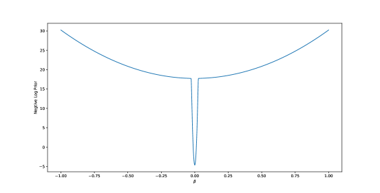
Figure 2: Negative logarithm of the mixture Gaussian prior.

Figure 3 shows the shape of negative log-prior and $\pi({\boldsymbol{\gamma}}_{i}=1|{\boldsymbol{\beta}}_{i})$ for different choices of $\sigma_{0,n}^{2}$ and $\lambda_{n}$. As we can see from the plot, $\sigma_{0,n}^{2}$ plays the major role in determining the effect of the prior. Let $\alpha$ be the threshold in step (iii) of Algorithm 1 of the main body, i.e. the positive solution to $\pi({\boldsymbol{\gamma}}_{i}=1|{\boldsymbol{\beta}}_{i})=0.5$. In general, a smaller $\sigma_{0,n}^{2}$ will result in a smaller $\alpha$. If a very small $\sigma_{0,n}^{2}$ is used in the prior from the beginning, then most of ${\boldsymbol{\beta}}_{i}$’s at initialization will have a magnitude larger than $\alpha$ and the slab component $N(0,\sigma_{1,n}^{2})$ of the prior will dominate most parameters. As a result, it will be difficult to find the desired sparse structure. Following the proposed prior annealing procedure, we can start with a larger $\sigma_{0,n}^{2}$, i.e. a larger threshold $\alpha$ and a relatively smaller penalty for those $|{\boldsymbol{\beta}}_{i}|<\alpha$. As we gradually decrease the value of $\sigma_{0,n}^{2}$, $\alpha$ decreases, and the penalty imposed on the small weights increases and drives them toward zero. The prior annealing allows us to gradually sparsify the DNN and impose more and more penalties on the parameters close to 0.

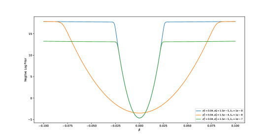
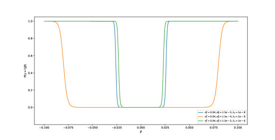
Figure 3: Negative log-prior and $\pi({\boldsymbol{\gamma}}=1|{\boldsymbol{\beta}})$ for different choices of $\sigma_{0,n}^{2}$ and $\lambda_{n}$.

A.6 Experimental Setups

A.6.1 Simulated examples

Prior annealing

We follow simple implementation of Algorithm given in section 3.1. We run SGHMC for $T=80000$ iterations with constant learning rate $\epsilon_{t}=0.001$, momentum $1-\alpha=0.9$ and subsample size $m=500$. We set $\lambda_{n}=1e-7,\sigma_{1,n}^{2}=1e-2$, $(\sigma_{0,n}^{init})^{2}=5e-5$, $(\sigma_{0,n}^{end})^{2}=1e-6$ and $T_{1}=5000,T_{2}=20000,T_{3}=60000$. We set temperature $\tau=0.1$ for $t<T_{3}$ and for $t>T_{3}$, we gradually decrease temperature $\tau$ by $\tau=\frac{0.1}{t-T_{3}}$. After structure selection, the model is fine tuned for 40000 iterations. The number of iteration setup is the same as Sun et al. [2021].

Other Methods

Spinn, Dropout and DNN are trained with the same network structure using SGD with momentum. Same as our method, we use constant learning rate $0.001$, momentum $0.9$, subsample size $500$ and traing the model for 80000 iterations. For Spinn, we use LASSO penalty and the regularization parameter is selected from $\{0.05,0.06,\dots,0.15\}$ according to the performance on validation data set. For Dropout, the dropout rate is set to be $0.2$ for the first layer and $0.5$ for the other layers. Other baseline methods BART50, LASSO, SIS are implemented using R-package $randomForest$, $glmnet$, $BART$ and $SIS$ respectively with default parameters.

A.6.2 CIFAR10

We follow the standard training procedure as in Lin et al. [2020], i.e. we train the model with SGHMC for $T=300$ epochs, with initial learning rate $\epsilon_{0}=0.1$, momentum $1-\alpha=0.9$, temperature $\tau=0.001$, mini-batch size $m=128$. The learning rate is divided by 10 at $150$th and $225$th epoch. We follow the implementation given in section 3.1 and use $T_{1}=150,T_{2}=200,T_{3}=225$, where $T_{i}$s are number of epochs. We set temperature $\tau=0.01$ for $t<T_{3}$ and gradually decrease $\tau$ by $\tau=\frac{0.01}{t-T_{3}}$ for $t>T_{3}$. We set $\sigma_{1,n}^{2}=0.04$ and $(\sigma_{0,n}^{init})^{2}=10\times(\sigma_{0,n}^{end})^{2}$ and use different $\sigma_{0,n}^{end},\lambda_{n}$ for different network size and target sparsity level. The detailed settings are given below:

• ResNet20 with target sparsity level 20%: $(\sigma_{0,n}^{end})^{2}=1.5e-5,\lambda_{n}=1e-8$

• ResNet20 with target sparsity level 10%: $(\sigma_{0,n}^{end})^{2}=6e-5,\lambda_{n}=1e-9$

• ResNet32 with target sparsity level 10%: $(\sigma_{0,n}^{end})^{2}=3e-5,\lambda_{n}=2e-9$

• ResNet32 with target sparsity level 5%: $(\sigma_{0,n}^{end})^{2}=1e-4,\lambda_{n}=2e-8$

References

- Allen-Zhu et al. [2019] Zeyuan Allen-Zhu, Yuanzhi Li, and Zhao Song. A convergence theory for deep learning via over-parameterization. In ICML, 2019.
- Bleich et al. [2014] Justin Bleich, Adam Kapelner, Edward I George, and Shane T Jensen. Variable selection for bart: an application to gene regulation. The Annals of Applied Statistics, pages 1750–1781, 2014.
- Bölcskei et al. [2019] Helmut Bölcskei, Philipp Grohs, Gitta Kutyniok, and Philipp Petersen. Optimal approximation with sparsely connected deep neural networks. CoRR, abs/1705.01714, 2019.
- Castillo and Rousseau [2015] Ismaël Castillo and Judith Rousseau. Supplement to “a bernstein–von mises theorem for smooth functionals in semiparametric models”. Annals of Statistics, 43(6):2353–2383, 2015.
- Castillo et al. [2015] Ismaël Castillo, Judith Rousseau, et al. A bernstein–von mises theorem for smooth functionals in semiparametric models. The Annals of Statistics, 43(6):2353–2383, 2015.
- Chen et al. [2015] Changyou Chen, Nan Ding, and Lawrence Carin. On the convergence of stochastic gradient mcmc algorithms with high-order integrators. In Proceedings of the 28th International Conference on Neural Information Processing Systems-Volume 2, pages 2278–2286, 2015.
- Chen et al. [2014] Tianqi Chen, Emily Fox, and Carlos Guestrin. Stochastic gradient hamiltonian monte carlo. In International conference on machine learning, pages 1683–1691, 2014.
- Dettmers and Zettlemoyer [2019] Tim Dettmers and Luke Zettlemoyer. Sparse networks from scratch: Faster training without losing performance. arXiv preprint arXiv:1907.04840, 2019.
- Du et al. [2019] Simon S. Du, Jason D. Lee, Haochuan Li, Liwei Wang, and Xiyu Zhai. Gradient descent finds global minima of deep neural networks. In ICML, 2019.
- Fan and Lv [2008] Jianqing Fan and Jinchi Lv. Sure independence screening for ultrahigh dimensional feature space. Journal of the Royal Statistical Society: Series B (Statistical Methodology), 70(5):849–911, 2008.
- Fefferman [1994] Charles Fefferman. Reconstructing a neural net from its output. Revista Matemática Iberoamericana, 10(3):507–555, 1994.
- Feng and Simon [2017] Jean Feng and Noah Simon. Sparse-input neural networks for high-dimensional nonparametric regression and classification. arXiv preprint arXiv:1711.07592, 2017.
- Gal and Ghahramani [2016] Yarin Gal and Zoubin Ghahramani. Dropout as a bayesian approximation: Representing model uncertainty in deep learning. In Proceedings of the 33rd International Conference on International Conference on Machine Learning - Volume 48, ICML’16, page 1050–1059. JMLR.org, 2016.
- Gori and Tesi [1992] M. Gori and A. Tesi. On the problem of local minima in backpropagation. IEEE Transactions on Pattern Analysis and Machine Intelligence, 14(1):76–86, 1992.
- Guo et al. [2017] Chuan Guo, Geoff Pleiss, Yu Sun, and Kilian Q. Weinberger. On calibration of modern neural networks. In Proceedings of the 34th International Conference on Machine Learning - Volume 70, ICML’17, page 1321–1330. JMLR.org, 2017.
- He et al. [2016] Kaiming He, Xiangyu Zhang, Shaoqing Ren, and Jian Sun. Deep residual learning for image recognition. In Proceedings of the IEEE conference on computer vision and pattern recognition, pages 770–778, 2016.
- Kingma and Ba [2015] D.P. Kingma and J.L. Ba. Adam: a method for stochastic optimization. In International Conference on Learning Representations, 2015.
- Krizhevsky et al. [2009] Alex Krizhevsky, Geoffrey Hinton, et al. Learning multiple layers of features from tiny images. Technical report, Citeseer, 2009.
- Lakshminarayanan et al. [2017] Balaji Lakshminarayanan, Alexander Pritzel, and Charles Blundell. Simple and scalable predictive uncertainty estimation using deep ensembles. In Proceedings of the 31st International Conference on Neural Information Processing Systems, NIPS’17, page 6405–6416, Red Hook, NY, USA, 2017. Curran Associates Inc. ISBN 9781510860964.
- Liang et al. [2013] F. Liang, Q. Song, and K. Yu. Bayesian subset modeling for high dimensional generalized linear models. Journal of the American Statistical Association, 108:589–606, 2013.
- Liang et al. [2018] F. Liang, Q. Li, and L. Zhou. Bayesian neural networks for selection of drug sensitive genes. Journal of the American Statistical Association, 113(523):955–972, 2018.
- Lin et al. [2020] Tao Lin, Sebastian U. Stich, Luis Barba, Daniil Dmitriev, and Martin Jaggi. Dynamic model pruning with feedback. In International Conference on Learning Representations, 2020. URL https://openreview.net/forum?id=SJem8lSFwB.
- Ma et al. [2015] Yi-An Ma, Tianqi Chen, and Emily Fox. A complete recipe for stochastic gradient mcmc. In Advances in Neural Information Processing Systems, pages 2917–2925, 2015.
- Maddox et al. [2019] Wesley J Maddox, Pavel Izmailov, Timur Garipov, Dmitry P Vetrov, and Andrew Gordon Wilson. A simple baseline for bayesian uncertainty in deep learning. In Advances in Neural Information Processing Systems, pages 13153–13164, 2019.
- Mostafa and Wang [2019] Hesham Mostafa and Xin Wang. Parameter efficient training of deep convolutional neural networks by dynamic sparse reparameterization. In International Conference on Machine Learning, pages 4646–4655, 2019.
- Nemeth and Fearnhead [2019] Christopher Nemeth and Paul Fearnhead. Stochastic gradient markov chain monte carlo. arXiv preprint arXiv:1907.06986, 2019.
- Nguyen and Hein [2017] Quynh Nguyen and Matthias Hein. The loss surface of deep and wide neural networks. In ICML, 2017.
- Polson and Ročková [2018] Nicholas G. Polson and Veronika Ročková. Posterior concentration for sparse deep learning. In Proceedings of the 32nd International Conference on Neural Information Processing Systems, NIPS’18, page 938–949, Red Hook, NY, USA, 2018. Curran Associates Inc.
- Portnoy [1988] S. Portnoy. Asymptotic behavior of likelihood methods for exponential families when the number of parameters tend to infinity. The Annals of Statistics, 16(1):356–366, 1988.
- Schmidt-Hieber [2017] Johannes Schmidt-Hieber. Nonparametric regression using deep neural networks with relu activation function. arXiv:1708.06633, 2017.
- Sun et al. [2021] Y. Sun, Q. Song, and F. Liang. Consistent sparse deep learning: Theory and computation. Journal of the American Statistical Association, page in press, 2021.
- Tibshirani [1996] Robert Tibshirani. Regression shrinkage and selection via the lasso. Journal of the Royal Statistical Society. Series B (Methodological), pages 267–288, 1996.
- Wang and Rocková [2020] Yuexi Wang and V. Rocková. Uncertainty quantification for sparse deep learning. In AISTATS, 2020.
- Welling and Teh [2011] Max Welling and Yee W Teh. Bayesian learning via stochastic gradient langevin dynamics. In Proceedings of the 28th international conference on machine learning (ICML-11), pages 681–688, 2011.
- Zou and Gu [2019] Difan Zou and Quanquan Gu. An improved analysis of training over-parameterized deep neural networks. In NuerIPS, 2019.
- Zou et al. [2020] Difan Zou, Yuan Cao, Dongruo Zhou, and Quanquan Gu. Gradient descent optimizes over-parameterized deep relu networks. Machine Learning, 109:467 – 492, 2020.