Factored couplings in multi-marginal optimal transport via difference of convex programming

Abstract

Optimal transport (OT) theory underlies many emerging machine learning (ML) methods nowadays solving a wide range of tasks such as generative modeling, transfer learning and information retrieval. These latter works, however, usually build upon a traditional OT setup with two distributions, while leaving a more general multi-marginal OT formulation somewhat unexplored. In this paper, we study the multi-marginal OT (MMOT) problem and unify several popular OT methods under its umbrella by promoting structural information on the coupling. We show that incorporating such structural information into MMOT results in an instance of a difference of convex (DC) programming problem allowing us to solve it numerically. Despite high computational cost of the latter procedure, the solutions provided by DC optimization are usually as qualitative as those obtained using currently employed optimization schemes.

1 Introduction

Broadly speaking, the classic OT problem provides a principled approach for transporting one probability distribution onto another following the principle of the least effort. Such a problem, and the distance on the space of probability distributions derived from it, arise in many areas of machine learning (ML) including generative modeling, transfer learning and information retrieval, where OT has been successfully applied. A natural extension of classic OT, in which the admissible transport plan (a.k.a coupling) can have more than two prescribed marginal distributions, is called the multi-marginal optimal transport (MMOT) (Gangbo and Swiech, 1998). The latter has several attractive properties: it enjoys a duality theory (Kellerer, 1984) and finds connections with the probabilistic graphical models (Haasler et al., 2020) and the Wasserstein barycenter problem (Agueh and Carlier, 2011) used for data averaging. While being less popular than the classic OT with two marginals, MMOT is a very useful framework on its own with some notable recent applications in generative adversarial networks (Cao et al., 2019), clustering (Mi and Bento, 2020) and domain adaptation (Hui et al., 2018; He et al., 2019), to name a few.

The recent success of OT in ML is often attributed to the entropic regularization (Cuturi, 2013) where the authors imposed a constraint on the coupling matrix forcing it to be closer to the independent coupling given by the rank-one product of the marginals. Such a constraint leads to the appearance of the strongly convex entropy term in the objective function and allows the entropic OT problem to be solved efficiently using simple Sinkhorn-Knopp matrix balancing algorithm. In addition to this, it was also noticed that structural constraints on the coupling and cost matrices allow to reduce the high computational cost and sample complexity of the classic OT problem (Genevay et al., 2019; Forrow et al., 2019; Lin et al., 2021; Scetbon et al., 2021). However, none of these works considered a much more challenging case of doing so in a multi-marginal setting. On the other hand, while the work of (Haasler et al., 2020) considers the MMOT problem in which the cost tensor induced by a graphical structure, it does not naturally promote the factorizability of transportation plans.

Contributions

In this paper, we define and study a general MMOT problem with structural penalization on the coupling matrix. We start by showing that a such formulation includes several popular OT methods as special cases and allows to gain deeper insights into them. We further consider a relaxed problem where the hard constraint is replaced by a regularization term and show that it leads to an instance of the difference of convex programming problem. A numerical study of the solutions obtained when solving the latter in cases of interest highlights their competitive performance when compared to solutions provided by the optimization strategies used previously.

2 Preliminary knowledge

Notations.

For each integer $n\geq 1$, we write $[n]:=\{1,...,n\}$. For any discrete probability measure $\mu$ with finite support, its negative entropy is defined as $H(\mu)=\langle\mu,\log\mu\rangle$, where the logarithm operator is element-wise, with the convention that $0\log 0=0$. Here, $\langle\cdot,\cdot\rangle$ denotes the Frobenius inner product. The Kullback-Leibler divergence between two discrete probability measures $\mu$ and $\nu$ with finite supports is defined as

$$\text{KL}(\mu|\nu)=\begin{cases}\langle\mu,\log\frac{\mu}{\nu}\rangle,\text{ if }\mu\text{ is absolutely continuous with respect to }\nu\\ \infty,\text{ otherwise}.\end{cases}$$

where the division operator in the logarithm is element-wise.

In what follows, given an integer $N\geq 1$, for any positive integers $a_{1},...,a_{N}$, we call $P\in\mathbb{R}^{a_{1}\times...\times a_{N}}$ a $N$-D tensor. In particular, a $1$-D tensor is a vector and $2$-D tensor is a matrix. A tensor is a probability tensor if its entries are nonnegative and the sum of all entries is $1$. Given $N$ probability vectors $\mu_{1},...,\mu_{N}$, we write $\mu=(\mu_{n})_{n=1}^{N}$. We denote $\Sigma$ the set of $N$-D probability tensors and $U(\mu)\subset\Sigma$ the set of nonnegative tensors whose $N$ marginal distributions are $\mu_{1},...,\mu_{N}$. In this case, any coupling in $U(\mu)$ is said to be admissible.

Multi-marginal OT problem.

Given a collection of $N$ probability vectors $\mu=(\mu_{n}\in\mathbb{R}^{a_{n}})_{n=1}^{N}$ and a $N$-D cost tensor $C\in\mathbb{R}^{a_{1}\times...\times a_{N}}$, the MMOT problem reads

$$\text{MMOT}(\mu)=\inf_{P\in U(\mu)}\langle C,P\rangle.$$

In practice, such a formulation is intractable to optimize in a discrete setting as it results in a linear program where the number of constraints grows exponentially in $N$. A more tractable strategy for solving MMOT is to consider the following entropic regularization problem

$$\inf_{P\in U(\mu)}\langle C,P\rangle+\varepsilon H(P).$$ (1)

which can be solved using Sinkhorn’s algorithm (Benamou et al., 2014). We refer the interested reader to Supplementary materials for algorithmic details.

3 Factored Multi-marginal Optimal Transport

In this section, we first define a factored MMOT (F-MMOT) problem where we seek to promote a structure on the optimal coupling given such as a factorization into a tensor product. Interestingly, such a formulation can be shown to include several other OT problems as special cases. Then, we introduce a relaxed version called MMOT-DC where the factorization constraint is smoothly promoted through a Kullback-Leibler penalty.

3.1 Motivation

Before a formal statement of our problem, we first give a couple of motivating examples showing why and when structural constraints on the coupling matrix can be beneficial. To this end, first note that a trivial example of the usefulness of such constraints in OT is the famous entropic regularization. Indeed, while most of the works define the latter by adding negative entropy of the coupling to the classic OT objective function directly, the original idea was to constraint the sought coupling to remain close (to some extent) to a rank-one product of the two marginal distributions. The appearance of negative entropy in the final objective function is then only a byproduct of such constraint due to the decomposition of the KL divergence into a sum of three terms with two of them being constant. Below we give two more examples of real-world applications related to MMOT problem where a certain decomposition imposed on the coupling tensor can be desirable.

Multi-source multi-target translation.

A popular task in computer vision is to match images across different domains in order to perform the so-called image translation. Such tasks are often tackled within the GAN framework where one source domain from which the translation is performed, is matched with multiple target domains modeled using generators. While MMOT was applied in this context by (Cao et al., 2019) when only one source was considered, its application in a multi-source setting may benefit from structural constraints on the coupling tensor incorporating the human prior on what target domains each source domain should be matched to.

Multi-task reinforcement learning.

In this application, the goal is to learn individual policies for a set of agents while taking into account the similarities between them and hoping that the latter will improve the individual policies. A common approach is to consider an objective function consisting of two terms where the first term is concerned with learning individual policies, while the second forces a consensus between them. Similar to the example considered above, MMOT problem was used to promote the consensus across different agents’ policies in (Cohen et al., 2021), even though such a consensus could have benefited from a prior regarding the semantic relationships between the learned tasks.

3.2 Factored MMOT and its relaxation

We start by giving several definitions used in the following parts of the paper.

Definition 3.1 (Tuple partition)

Given two integers $N\geq M\geq 2$, a sequence of tuples $\mathcal{T}=(\mathcal{T}_{m})_{m=1}^{M}$, is called a tuple partition of the $N$-tuple $(1,...,N)$ if the tuples $\mathcal{T}_{1},...,\mathcal{T}_{M}$ are nonempty and disjoint, and their concatenation in this order gives $(1,...,N)$.

Here, we implicitly take into account the order of the tuple, which is not the case for the partition of the set $[N]$. If there exists a tuple in $\mathcal{T}$ which contains only one element, then we say $\mathcal{T}$ is degenerate.

Definition 3.2 (Marginal tensor)

Given a tensor $P\in\mathbb{R}^{a_{1}\times...\times a_{N}}$ and a tuple partition $\mathcal{T}=(\mathcal{T}_{m})_{m=1}^{M}$, we call $P_{\#\mathcal{T}_{m}}$ its $\mathcal{T}_{m}$-marginal tensor, by summing $P$ over all dimensions not in $\mathcal{T}_{m}$. We write $P_{\#\mathcal{T}}=P_{\#\mathcal{T}_{1}}\otimes...\otimes P_{\#\mathcal{T}_{M}}\in\mathbb{R}^{a_{1}\times...\times a_{N}}$ the tensor product of its marginal tensors.

For example, for $M=N=2$, we have $\mathcal{T}_{1}=(1)$ and $\mathcal{T}_{2}=(2)$. So, given a matrix $P\in\mathbb{R}^{a_{1}\times a_{2}}$, its marginal tensors $P_{\#\mathcal{T}_{1}}$ and $P_{\#\mathcal{T}_{2}}$ are simply vectors in $\mathbb{R}^{a_{1}}$ and $\mathbb{R}^{a_{2}}$, respectively, defined by $(P_{\#\mathcal{T}_{1}})_{i}=\sum_{j}P_{ij}$ and $(P_{\#\mathcal{T}_{2}})_{j}=\sum_{i}P_{ij}$ for $(i,j)\in[a_{1}]\times[a_{2}]$. The tensor product $P_{\#\mathcal{T}}\in\mathbb{R}^{a_{1}\times a_{2}}$ is then defined by $(P_{\#\mathcal{T}})_{ij}=(P_{\#\mathcal{T}_{1}})_{i}(P_{\#\mathcal{T}_{2}})_{j}$.

Clearly, if $P$ is a probability tensor, then so are its marginal tensors and tensor product.

Suppose $\mathcal{T}_{m}=(p,...,q)$ for some $m\in[M]$ and $1\leq p\leq q\leq N$. We denote $\Sigma_{\mathcal{T}_{m}}$ the set of probability tensors in $\mathbb{R}^{a_{p}\times...\times a_{q}}$ and $U_{\mathcal{T}_{m}}\subset\Sigma_{\mathcal{T}_{m}}$ the set of probability tensors in $\mathbb{R}^{a_{p}\times...\times a_{q}}$ whose $(r)$-marginal vector is $\mu_{r}$, for every $r=p,...,q$.

Definition 3.3 (Factored MMOT)

Given a collection of histograms $\mu=(\mu_{n})_{n=1}^{N}$ and a tuple partition $\mathcal{T}=(\mathcal{T}_{m})_{m=1}^{M}$, we consider the following OT problem

$$\text{F-MMOT}(\mathcal{T},\mu)=\inf_{P\in U_{\mathcal{T}}}\langle C,P\rangle,$$ (2)

where $U_{\mathcal{T}}\subset U(\mu)$ is the set of admissible couplings which can be factorized as a tensor product of $M$ component probability tensors in $\Sigma_{\mathcal{T}_{1}},...,\Sigma_{\mathcal{T}_{M}}$.

Several remarks are in order here. First, one should note that the partition considered above is in general not degenerate meaning that the decomposition can involve tensors of an arbitrary order $<N$. Second, the decomposition in this setting depicts the prior knowledge regarding the tuples of measures which should be independent: the couplings for the measures from different tuples will be degenerate and the optimal coupling tensor will be reconstructed from couplings of each tuple separately. Third, suppose the partition $(\mathcal{T}_{m})_{m=1}^{M}$ is not degenerate and $M=2$, i.e. the tensor is factorized as product of two tensors, the problem 2 is equivalent to a variation of low nonnegative rank OT problem (see Appendix for a proof).

As for the existence of the solution to this problem, we have that $U_{\mathcal{T}}$ is compact because it is a close subset of the compact set $U(\mu)$, which implies that the problem 2 always admits a solution. Furthermore, observe that

$$\begin{split}U_{\mathcal{T}}&=\{P\in U(\mu):P=P_{1}\otimes...\otimes P_{M},\text{where }P_{m}\in\Sigma_{\mathcal{T}_{m}},\forall m=1,...,M\}\\ &=\{P\in\Sigma:P=P_{1}\otimes...\otimes P_{M},\text{where }P_{m}\in U_{\mathcal{T}_{m}},\forall m=1,...,M\}.\end{split}$$

Thus, the problem F-MMOT can be rewritten as

$$\text{F-MMOT}(\mathcal{T},\mu)=\inf_{\begin{subarray}{c}P_{m}\in U_{\mathcal{T}_{m}}\\ \forall m=1,...,M\end{subarray}}\langle C,P_{1}\otimes...\otimes P_{M}\rangle.$$

So, if $\mathcal{T}_{1},...,\mathcal{T}_{M}$ are $2$-tuples and two marginal distributions corresponding to each $U_{\mathcal{T}_{m}}$ are identical and uniform, then by Birkhoff’s theorem (Birkhoff, 1946), the problem 2 admits an optimal solution in which each component tensor $P_{m}$ is a permutation matrix.

Two special cases.

When $N=4$ and $M=2$ with $\mathcal{T}_{1}=(1,2)$ and $\mathcal{T}_{2}=(3,4)$, the problem 2 becomes the CO-Optimal transport (COOT) (Redko et al., 2020), where the two component tensors are known as sample and feature couplings. If furthermore, $a_{1}=a_{3},a_{2}=a_{4}$, and $\mu_{1}=\mu_{3},\mu_{2}=\mu_{4}$, it becomes a lower bound of the discrete Gromov-Wasserstein (GW) distance (Mémoli, 2011). This means that our formulation can be seen as a generalization of several OT formulations.

Observe that if a probability tensor $P$ can be factorized as a tensor product of probability tensors, i.e. $P=P_{1}\otimes...\otimes P_{M}$, then each $P_{m}$ is also the $\mathcal{T}_{m}$-marginal tensor of $P$. In this case, we have $P=P_{\#\mathcal{T}}$. This prompts us to consider the following relaxation of factored MMOT, where the hard constraint $U_{\mathcal{T}}$ is replaced by a regularization term.

Definition 3.4 (Relaxed Factored MMOT)

Given $\varepsilon\geq 0$, a collection of measures $\mu$ and a tuple partition $\mathcal{T}$, we define the following problem:

$$\text{MMOT-DC}_{\varepsilon}(\mathcal{T},\mu)=\inf_{P\in U(\mu)}\langle C,P\rangle+\varepsilon\text{KL}(P|P_{\#\mathcal{T}}).$$ (3)

From the exposition above, one can guess that this relaxation is reminiscent of the entropic regularization in MMOT and coincides with it when $M=N$. As such, it also recovers the classical entropic OT. One should note that the choice of the KL divergence is not arbitrary and its advantage will become clear when it comes to the algorithm. A special case of the problem 3 is when $M=N$, we recover the entropic-regularized MMOT problem, up to a constant.

After having defined the two optimization problems, we now set on exploring their theoretical properties.

3.3 Theoretical properties

Intuitively, the relaxed problem is expected to allow for solutions with a lower value of the final objective function. We formally prove the validity of this intuition below.

Proposition 3.1 (Preliminary properties)

Given a collection of histograms $\mu$ and a tuple partition $\mathcal{T}$,

1. For every $\varepsilon\geq 0$, we have $\text{MMOT}(\mu)\leq\text{MMOT-DC}_{\varepsilon}(\mathcal{T},\mu)\leq\text{F-MMOT}(\mathcal{T},\mu)$.

2. For every $\varepsilon>0,\text{MMOT-DC}_{\varepsilon}(\mathcal{T},\mu)=0$ if and only if $\text{F-MMOT}(\mathcal{T},\mu)=0$.

An interesting property of MMOT-DC is that it interpolates between MMOT and F-MMOT. Informally, for very large $\varepsilon$, the KL divergence term dominates, so the optimal transport plans tend to be factorizable. On the other hand, for very small $\varepsilon$, the KL divergence term becomes negligible and we approach MMOT. The result below formalizes this intuition.

Proposition 3.2 (Interpolation between MMOT and F-MMOT)

For any tuple partition $\mathcal{T}$ and for $\varepsilon>0$, let $P_{\varepsilon}$ be a minimiser of the problem $\text{MMOT-DC}_{\varepsilon}(\mathcal{T},\mu)$.

1. When $\varepsilon\to\infty$, one has $\text{MMOT-DC}_{\varepsilon}(\mathcal{T},\mu)\to\text{F-MMOT}(\mathcal{T},\mu)$. In this case, any cluster point of the sequence of minimisers $(P_{\varepsilon})_{\varepsilon}$ is a minimiser of $\text{F-MMOT}(\mathcal{T},\mu)$.

2. When $\varepsilon\to 0$, then $\text{MMOT-DC}_{\varepsilon}(\mathcal{T},\mu)\to\text{MMOT}(\mu)$. In this case, any cluster point of the sequence of minimisers $(P_{\varepsilon})_{\varepsilon}$ is a minimiser of $\text{MMOT}(\mu)$.

GW distance revisited.

Somewhat surprisingly, the relaxation 3 also allows us to prove the equality between GW distance and COOT in the discrete setting. Let $\mathcal{X}$ be a finite subset (of size $m$) of a certain metric space. Denote $C_{x}\in\mathbb{R}^{m\times m}$ its similarity matrix (e.g. distance matrix). We define similarly the set $\mathcal{Y}$ of size $n$ and the corresponding similarity matrix $C_{y}\in\mathbb{R}^{n\times n}$. We also assign two discrete probability measures $\mu_{x}\in\mathbb{R}^{m}$ and $\mu_{y}\in\mathbb{R}^{n}$ to $\mathcal{X}$ and $\mathcal{Y}$, respectively. The GW distance is then defined as

$$\text{GW}(C_{x},C_{y})=\inf_{Q\in U(\mu_{x},\mu_{y})}\langle L(C_{x},C_{y}),Q\otimes Q\rangle,$$

and the COOT reads

$$\text{COOT}(C_{x},C_{y})=\inf_{\begin{subarray}{c}Q_{s}\in U(\mu_{x},\mu_{y})\\ Q_{f}\in U(\mu_{x},\mu_{y})\end{subarray}}\langle L(C_{x},C_{y}),Q_{s}\otimes Q_{f}\rangle,$$

where $L(C_{x},C_{y})\in\mathbb{R}^{m\times n\times m\times n}$ represents the $4$-D cost tensor induced by the matrices $C_{x}$ and $C_{y}$, and $U(\mu,\nu)$ is the set of couplings in $\mathbb{R}^{m\times n}_{\geq 0}$ whose two marginal distributions are $\mu$ and $\nu$. When $C_{x}$ and $C_{y}$ are two squared Euclidean distance matrices, and $L(C_{x},C_{y})$ is of the form $\big{(}L(C_{x},C_{y})\big{)}_{i,j,k,l}=|(C_{x})_{i,k}-(C_{y})_{j,l}|^{2}$, it can be shown that the GW distance is equal to the COOT (Redko et al., 2020). This is also true when $L(C_{x},C_{y})$ is a negative definite kernel (Séjourné et al., 2020). Here, we establish a weaker case where this equality still holds.

Corollary 3.3

If $L(C_{x},C_{y})$ defines a conditionally negative definite kernel on $(\mathcal{X}\times\mathcal{Y})^{2}$, then we have the equality between GW distance and COOT. Furthermore, if $(Q_{s}^{*},Q_{f}^{*})$ is a solution of the COOT problem, then $Q_{s}^{*}$ and $Q_{f}^{*}$ are two solutions of the GW problem. In particular, when $L(C_{x},C_{y})$ induces a strictly positive definite kernel $\exp\big{(}-\frac{L(C_{x},C_{y})}{\varepsilon}\big{)}$, for every $\varepsilon>0$, we have $Q_{s}^{*}=Q_{f}^{*}$.

The proof relies on the connection between MMOT-DC and COOT shown in the proposition 3.2, and given a $4$-D solution of MMOT-DC, we can construct another $4$-D solutions whose $\mathcal{T}_{1}$ and $\mathcal{T}_{2}$-marginal matrices are identical, under the assumption of the cost tensor. The proof of the second claim is deferred to the Appendix.

4 Numerical solution

We now turn to the computational aspect of the problem 3. First, note that for any tuple partition $\mathcal{T}=(\mathcal{T}_{m})_{m=1}^{M}$ and probability tensor $P$, the KL divergence term can be decomposed as

$$\text{KL}(P|P_{\#\mathcal{T}})=H(P)-\sum_{m=1}^{m}H_{m}(P),$$

where the function $H_{m}$ defined by $H_{m}(P):=H(P_{\#\mathcal{T}_{m}})$ is continuous and convex with respect to $P$. Now, the problem 3 becomes

$$\text{MMOT-DC}_{\varepsilon}(\mathcal{T},\mu)=\inf_{P\in U(\mu)}\langle C,P\rangle+\varepsilon H(P)-\varepsilon\sum_{m=1}^{M}H_{m}(P).$$ (4)

This is nothing but a Difference of Convex (DC) programming problem (which explains the name MMOT-DC), thanks to the convexity of the set $U(\mu)$ and the entropy function $H$. Thus, it can be solved by the DC algorithm (Pham and Bernoussi, 1986; Pham and Le, 1997) as follows: at the iteration $t$,

1. Calculate $G^{(t)}\in\partial(\sum_{m=1}^{M}H_{m})(P^{(t)})$.

2. Solve $P^{(t+1)}\in\arg\min_{P\in U(\mu)}\langle C-\varepsilon G^{(t)},P\rangle+\varepsilon H(P)$.

This algorithm is very easy to implement. Indeed, the second step is an entropic-regularized MMOT problem, which admits a unique solution, thanks to the strict convexity of the objective function. Such solution can be found by the Sinkhorn algorithm 3. In the first step, the gradient can be calculated explicitly. For the sake of simplicity, we illustrate the calculation in a simple case, where $M=2$ and $N=4$ with $\mathcal{T}_{1}$ and $\mathcal{T}_{2}$ are two $2$-tuples. The function $H_{1}+H_{2}$ is continuous, so $G^{(t)}=\nabla_{P}(H_{1}+H_{2})(P^{(t)})$. Given a $4$-D probability tensor $P$, we have

$$H_{1}(P)+H_{2}(P)=\sum_{i,j,k,l}P_{i,j,k,l}\log\big{(}\sum_{i,j}P_{i,j,k,l}\big{)}+P_{i,j,k,l}\log\big{(}\sum_{k,l}P_{i,j,k,l}\big{)}.$$

So,

$$\frac{\partial(H_{1}+H_{2})}{\partial P_{i,j,k,l}}=\log\left(\sum_{i,j}P_{i,j,k,l}\right)+\frac{P_{i,j,k,l}}{\sum_{i,j}P_{i,j,k,l}}+\log\left(\sum_{k,l}P_{i,j,k,l}\right)+\frac{P_{i,j,k,l}}{\sum_{k,l}P_{i,j,k,l}}.$$

The complete DC algorithm for the problem 4 can be found in the algorithm 1.

Algorithm 1 DC algorithm for the problem 3.

Input. Cost tensor $C$, tuple partition $(\mathcal{T}_{m})_{m=1}^{M}$, collection of histograms $\mu=(\mu_{n})_{n=1}^{N}$, hyperparameter $\varepsilon>0$, initialization $P^{(0)}$, tuple of initial dual vectors for the Sinkhorn step $(f_{1}^{(0)},...,f_{N}^{(0)})$.

Output. Tensor $P\in U(\mu)$.

While not converge

1. Gradient step: compute the gradient of the convex term $G^{(t)}=\sum\limits_{m=1}^{M}\nabla_{P}H_{m}(P^{(t)})$.

2. Sinkhorn step: solve

   $$P^{(t+1)}=\arg\min_{P\in U(\mu)}\langle C-\varepsilon G^{(t)},P\rangle+\varepsilon H(P),$$

   using the Sinkhorn algorithm 3, with the tuple of initial dual vectors $(f_{1}^{(0)},...,f_{N}^{(0)})$.

We observed that initialization is crucial to the convergence of algorithm, which is not surprising for a non-convex problem. To accelerate the algorithm for large $\varepsilon$, we propose to use the warm-start strategy, which is similar to the one used in the entropic OT problem with very small regularization parameter (Schmitzer, 2019). Its idea is simple: we consider an increasing finite sequence $(\varepsilon_{n})_{n=0}^{N}$ approaching $\varepsilon$ such that the solution $P_{\varepsilon_{0}}$ of the problem $\text{MMOT-DC}_{\varepsilon_{0}}(\mathcal{T},\mu)$ can be estimated quickly and accurately using the initialization $P^{(0)}$. Then we solve each successive problem $\text{MMOT-DC}_{\varepsilon_{n}}(\mathcal{T},\mu)$ using the previous solution $P_{\varepsilon_{n-1}}$ as initialization. Finally, the problem $\text{MMOT-DC}_{\varepsilon}(\mathcal{T},\mu)$ is solved using the solution $P_{\varepsilon_{N}}$ as initialization.

Algorithm 2 DC algorithm with warm start for the problem 3.

Input. Cost tensor $C$, tuple partition $\mathcal{T}=(\mathcal{T}_{m})_{m=1}^{M}$, collection of histograms $\mu=(\mu_{n})_{n=1}^{N}$, hyperparameter $\varepsilon>0$, initialization $P^{(0)}$, initial $\varepsilon_{0}>0$, step size $s>1$, tuple of initial dual vectors $(f_{1}^{(0)},...,f_{N}^{(0)})$.

Output. Tensor $P\in U(\mu)$.

1. While $\varepsilon_{0}<\varepsilon$:

   1. Using algorithm 1, solve the problem $\text{MMOT-DC}_{\varepsilon_{0}}(\mathcal{T},\mu)$ with initialization $P^{(0)}$ and $(f_{1}^{(0)},...,f_{N}^{(0)})$ to find the solution $P_{\varepsilon_{0}}$ and its associated tuple of dual vectors $(f_{1}^{(\varepsilon_{0})},...,f_{N}^{(\varepsilon_{0})})$.

   2. Set $P^{(0)}=P_{\varepsilon_{0}},f_{i}^{(0)}=f_{i}^{(\varepsilon_{0})}$, for $i=1,...,N$.

   3. Increase regularization: $\varepsilon_{0}:=s\varepsilon_{0}$.

2. Using algorithm 1, solve the problem $\text{MMOT-DC}_{\varepsilon}(\mathcal{T},\mu)$ using the initialization $P^{(0)}$ and $(f_{1}^{(0)},...,f_{N}^{(0)})$.

5 Experimental evaluation

In this section, we illustrate the use of MMOT-DC on simulated data. Rather than performing experiments in full generality, we choose the setting where $N=4$ and $M=2$ with $\mathcal{T}_{1}=(1,2)$ and $\mathcal{T}_{2}=(3,4)$, so that we can compare MMOT-DC with other popular solvers of COOT and GW distance. Given two matrices $X$ and $Y$, we always consider the $4$-D cost tensor $C$, where $C_{i,j,k,l}=|X_{i,k}-Y_{j,l}|^{2}$. On the other hand, we are not interested in the $4$-D minimiser of MMOT-DC, but only in its two $\mathcal{T}_{1},\mathcal{T}_{2}$-marginal matrices.

Solving COOT on a toy example.

We generate a random matrix $X\in\mathbb{R}^{30\times 25}$, whose entries are drawn independently from the uniform distribution on the interval $[0,1)$. We equip the rows and columns of $X$ with two discrete uniform distributions on $[30]$ and $[25]$. We fix two permutation matrices $Q_{s}\in\mathbb{R}^{30\times 30}$ (called sample permutation) and $Q_{f}\in\mathbb{R}^{25\times 25}$ (called feature permutation), then calculate $Y=Q_{s}XQ_{f}$. We also equip the rows and columns of $Y$ with two discrete uniform distributions on $[30]$ and $[25]$.

It is not difficult to see that $\text{COOT}(X,Y)=0$ because $(Q_{s},Q_{f})$ is a solution. As COOT is a special case of F-MMOT, we see that $\text{MMOT-DC}_{\varepsilon}(\mathcal{T},\mu)=0$, for every $\varepsilon>0$, by proposition 3.1. In this experiment, we will check if marginalizing the minimizer of MMOT-DC allows us to recover the permutation matrices $Q_{s}$ and $Q_{f}$. As can be seen from the figure 1, MMOT-DC can recover the permutation positions, for various values of $\varepsilon$. On the other hand, it can not recover the true sparse permutation matrices because the Sinkhorn algorithm applied to the MMOT problem implicitly results in a dense tensor, thus having dense marginal matrices. For this reason, the loss only remains very close to zero, but never exactly.

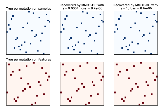
Figure 1: Couplings generated by COOT and MMOT-DC on the matrix recovering task.

We also plot, with some abuse of notation, the histograms of the difference between the $(1,3),(1,4),(2,3),(2,4)$-marginal matrices of MMOT-DC and their corresponding counterparts from F-MMOT. In this example, in theory, as the optimal tensor $P$ of F-MMOT can be factorized as $P=P_{\#\mathcal{T}_{1}}\otimes P_{\#\mathcal{T}_{2}}=Q_{s}\otimes Q_{f}$, it is immediate to see that $P_{\#(1,3)}=P_{\#(1,4)}=P_{\#(2,3)}=P_{\#(2,4)}\in\mathbb{R}^{30\times 25}$ are uniform matrices whose entries are $\frac{1}{750}$.

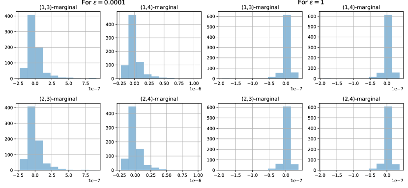
Figure 2: Histograms of difference between true independent marginal matrices and their approximations. We see that the marginal matrices obtained by the algorithm 1 approximate well the theoretical uniform matrices.

Quality of the MMOT-DC solutions.

Now, we consider the situation where the true matching between two matrices is not known in advance and investigate the quality of the solutions returned by MMOT-DC to solve the COOT and GW problems. This means that we will look at the COOT loss $\langle C,Q_{s}\otimes Q_{f}\rangle$, where the smaller the loss, the better when using both exact COOT and GW solvers and our relaxation.

We generate two random matrices $X\in\mathbb{R}^{20\times 3}$ and $Y\in\mathbb{R}^{30\times 2}$, whose entries are drawn independently from the uniform distribution on the interval $[0,1)$. Then we calculate two corresponding squared Euclidean distance matrices of size $20$ and $30$. Their rows and columns are equipped with the discrete uniform distributions. In this case, (Redko et al., 2020) show that the COOT loss coincides with the GW distance, and the Block Coordinate Descent (BCD) algorithm used to approximate COOT is equivalent to the Frank-Wolfe algorithm (Frank and Wolfe, 1956) used to solve the GW distance.

We compare four solvers:

1. The Frank-Wolfe algorithm to solve the GW distance (GW-FW).

2. The projected gradient algorithm to solve the entropic GW distance (Peyré et al., 2016) (EGW-PGD). We choose the regularization parameter from $\{0.0008,0.0016,0.0032,0.0064,0.0128,0.0256\}$ and pick the one which corresponds to smallest COOT loss.

3. The Block Coordinate Descent algorithm to approximate the entropic COOT (Redko et al., 2020) (EGW-BCD), where two additional KL divergences corresponding to two couplings are introduced. Both regularization parameters are tuned from $\{0,0.0005,0.001,0.005,0.01,0.05,0.1,0.5,1\}$, where $0$ means that there is no regularization term for the corresponding coupling and we pick the pair whose COOT loss is the smallest.

4. The algorithm 1 to solve the MMOT-DC. We tune $\varepsilon\in\{1,1.4,1.8,2.2,2.6\}$ and we pick the one which corresponds to smallest COOT loss.

For GW-FW and EGW-PGD, we use the implementation from the library PythonOT (Flamary et al., 2021).

Given two random matrices, we record the COOT loss corresponding to the solution generated by each method. We simulate this process $70$ times and compare their overall performance. We can see in Table 1 the average value and standard deviation and the comparison for the values of the loss between the different algorithms in Figure 3. The performance is quite similar across methods with a slight advantage for EGW-PGD. This is in itself a very interesting result that has never been noted, to the best of our knowledge: the reason that the entropic version of GW can provide better solution than solving the exact problem, may be due to the "convexification" of the problem, thanks to the entropic regularization. Our approach is also interestingly better than the exact GW-FW, which illustrates that the relaxation might help in finding better solutions despite the non-convexity of the problem.

GW-FW	EGW-PGD	EGW-BCD	MMOT-DC
0.0829 ($\pm$ 0.0354)	0.0786 ($\pm$ 0.0347)	0.0804 ($\pm$ 0.0353)	0.0822 ($\pm$ 0.0364)

Table 1: Average and standard deviation of COOT loss of the solvers. MMOT-DC is competitive to other solvers, except for EGW-PGD and EGW-BCD.

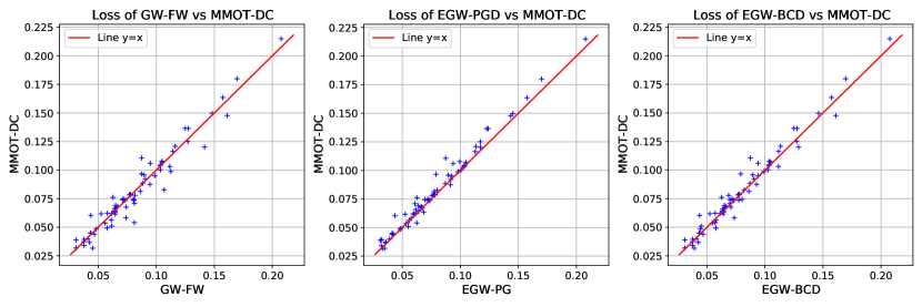
Figure 3: Scatter plots of MMOT-DC versus other solvers. In all three plots, the points tend to concentrate around the line $y=x$, which indicates the comparable performance of MMOT-DC. On the other hand, the top-right plot shows the clear superiority of EGW-PGD.

6 Discussion and conclusion

In this paper, we present a novel relaxation of the factorized MMOT problem called MMOT-DC. More precisely, we replace the hard constraint on factorization constraint by a smooth regularization term. The resulting problem not only enjoys an interpolation property between MMOT and factorized MMOT, but also is a DC problem, which can be solved easily by the DC algorithm. We illustrate the use of MMOT-DC the via some simulated experiments and show that it is competitive with the existing popular solvers of COOT and GW distance. One limitation of the current DC algorithm is that, it is not scalable because it requires storing a full-size tensor in the gradient step computation. Thus, future work may focus on more efficiently designed algorithms, in terms of both time and memory footprint. Moreover, incorporating additional structure on the cost tensor may also be computationally and practically beneficial. From a theoretical viewpoint, it is also interesting to study the extension of MMOT-DC to the continuous setting, which can potentially allow us to further understand the connection between GW distance and COOT.

Acknowledgements.

The authors thank to Thibault Séjourné and Titouan Vayer for the fruitful discussion on the GW distance. The authors thank the anonymous reviewers for their careful proofreading and invaluable suggestions. This work is partially funded by the projects OATMIL ANR-17-CE23-0012, OTTOPIA ANR-20-CHIA-0030 and 3IA Côte d’Azur Investments ANR-19-P3IA-0002 of the French National Research Agency (ANR). This research was produced within the framework of Energy4Climate Interdisciplinary Center (E4C) of IP Paris and Ecole des Ponts ParisTech. This research was supported by the 3rd Programme d’Investissements d’Avenir ANR-18-EUR-0006-02. This action benefited from the support of the Chair "Challenging Technology for Responsible Energy" led by l’X – Ecole Polytechnique and the Fondation de l’Ecole Polytechnique, sponsored by TOTAL, and the Chair "Business Analytics for Future Banking" sponsored by NATIXIS.

Appendix A Appendix

Derivation of the Sinkhorn algorithm in entropic MMOT.

The corresponding entropic dual problem of the primal problem 1 reads

$$\sup_{f_{n}\in\mathbb{R}^{a_{n}}}\sum_{n=1}^{N}\langle f_{n},\mu_{n}\rangle-\varepsilon\sum_{i_{1},...,i_{N}}\exp\Big{(}\frac{\sum_{n}(f_{n})_{i_{n}}-C_{i_{1},...,i_{N}}}{\varepsilon}\Big{)}+\varepsilon.$$

For each $n\in[N]$ and $i_{n}\in[a_{n}]$, the first order optimality condition reads

$$0=(\mu_{n})_{i_{n}}-\exp\big{(}\frac{(f_{n})_{i_{n}}}{\varepsilon}\big{)}\sum_{i_{-n}}\exp\Big{(}\frac{\sum_{j\neq n}(f_{j})_{i_{j}}-C_{i_{1},...,i_{N}}}{\varepsilon}\Big{)},$$

where, with some abuse of notation, we write $i_{-n}=(i_{1},...,i_{n-1},i_{n+1},...,i_{N})$. Or, equivalently

$$(f_{n})_{i_{n}}=\varepsilon\log(\mu_{n})_{i_{n}}-\varepsilon\log\sum_{i_{-n}}\exp\Big{(}\frac{\sum_{j\neq n}(f_{j})_{i_{j}}-C_{i_{1},...,i_{N}}}{\varepsilon}\Big{)},$$

or even more compact form

$$f_{n}=\varepsilon\log\mu_{n}-\varepsilon\log\sum_{i_{-n}}\exp\Big{(}\frac{\sum_{j\neq n}(f_{j})_{i_{j}}-C_{\cdot,i_{-n}}}{\varepsilon}\Big{)}.$$

Using the primal-dual relation, we obtain the minimiser of the primal problem 1 by

$$P_{i_{1},...,i_{N}}=\exp\Big{(}\frac{\sum_{n}(f_{n})_{i_{n}}-C_{i_{1},...,i_{N}}}{\varepsilon}\Big{)},$$

for $i_{n}\in[a_{n}]$, with $n\in[N]$. Similar to the entropic OT, the Sinkhorn algorithm 3 is also usually implemented in log-domain to avoid numerical instability.

Algorithm 3 Sinkhorn algorithm for the entropic MMOT problem 1 from [Benamou et al., 2014].

Input. Histograms $\mu_{1},...,\mu_{N}$, hyperparameter $\varepsilon>0$, cost tensor $C$ and tuple of initial dual vectors $(f^{(0)}_{1},...f^{(0)}_{N})$.

Output. Optimal transport plan $P$ and tuple of dual vectors $(f_{1},...f_{N})$ (optional).

1. While not converge: for $n=1,...,N$,

   $$\begin{split}f^{(t+1)}_{n}&=\varepsilon\log\mu_{n}-\varepsilon\log\sum_{i_{-n}}\Big{[}\exp\Big{(}\frac{\sum_{j<n}(f^{(t+1)}_{j})_{i_{j}}+\sum_{j>n}(f^{(t)}_{j})_{i_{j}}-C_{\cdot,i_{-n}}}{\varepsilon}\Big{)}\Big{]}.\end{split}$$

2. Return tensor $P$, where for $i_{n}\in[a_{n}]$, with $n\in[N]$,

   $$P_{i_{1},...,i_{N}}=\exp\Big{(}\frac{\sum_{n}(f_{n})_{i_{n}}-C_{i_{1},...,i_{N}}}{\varepsilon}\Big{)}.$$

F-MMOT of two components (i.e. $M=2$) is a variation of low nonnegative rank OT.

For the sake of notational ease, we only consider the simplest case, where $N=4$ and $M=2$ with $\mathcal{T}_{1}=(1,2)$ and $\mathcal{T}_{2}=(3,4)$. However, the same argument still holds in the general case. First, we define three reshaping operations.

• vectorization: concatenates rows of a matrix into a vector.

  $$\text{vec}:\mathbb{R}^{m\times n}\to\mathbb{R}^{mn},$$

  where each element $A_{i,j}$ of the matrix $A\in\mathbb{R}^{m\times n}$ is mapped to a unique element $b_{(i-1)n+j}$ of the vector $b\in\mathbb{R}^{mn}$, with $A_{i,j}=b_{(i-1)n+j}$, for $i=1,...,m$ and $j=1,...,n$. Conversely, each element $b_{k}$ is mapped to a unique element $A_{k//n,n-k\%n}$, for every $k=1,...,mn$. Here, $k//n$ is the quotient of the division of $k$ by $n$ and $k\%n$ is the remainder of this division, i.e. if $k=qn+r$, with $0\leq r<n$, then $k//n=q$ and $k\%n=r$.

• Matrization: transforms a $4$D tensor to a $2$D tensor (matrix) by vectorizing the first two and the last two dimensions of the tensor.

  $$\text{mat}:\mathbb{R}^{n_{1}\times n_{2}\times n_{3}\times n_{4}}\to\mathbb{R}^{(n_{1}n_{2})\times(n_{3}n_{4})},$$

  where, similar to the vectorization, each element $P_{i,j,k,l}$ of the tensor $P\in\mathbb{R}^{n_{1}\times n_{2}\times n_{3}\times n_{4}}$ is mapped to the unique element $A_{(i-1)n_{2}+j,(k-1)n_{4}+l}$ of the matrix $A\in\mathbb{R}^{(n_{1}n_{2})\times(n_{3}n_{4})}$, with $P_{i,j,k,l}=A_{(i-1)n_{2}+j,(k-1)n_{4}+l}$.

• Concatenation: stacks vertically two equal-column matrices.

  $$\begin{split}\text{con}_{v}:&\mathbb{R}^{m\times d}\times\mathbb{R}^{n\times d}\to\mathbb{R}^{(m+n)\times d}\\ &\big{(}(u_{1},...,u_{m}),(v_{1},...,v_{n})\big{)}\to(u_{1},...,u_{m},v_{1},...,v_{n})^{T}.\end{split}$$

  Or, stacks horizontally two equal-row matrices

  $$\begin{split}\text{con}_{h}:&\mathbb{R}^{n\times p}\times\mathbb{R}^{n\times q}\to\mathbb{R}^{n\times(p+q)}\\ &\big{(}(u_{1},...,u_{p}),(v_{1},...,v_{q})\big{)}\to(u_{1},...,u_{p},v_{1},...,v_{q}).\end{split}$$

Lemma A.1

For any $4$-D tensor $P\in\mathbb{R}^{n_{1}\times n_{2}\times n_{3}\times n_{4}}$, denote $\pi$ its matrisation. We have,

$$\text{vec}\Big{(}\sum_{k,l}P_{\cdot,\cdot,k,l}\Big{)}=\sum_{n=1}^{n_{3}n_{4}}\pi_{\cdot,n}=\pi 1_{n_{3}n_{4}},$$

where $1_{n}$ is the vector of ones in $\mathbb{R}^{n}$.

Proof of lemma A.1.

For $(i,j)\in[n_{1}]\times[n_{2}]$, we have

$$\begin{split}\text{vec}\Big{(}\sum_{k,l}P_{\cdot,\cdot,k,l}\Big{)}_{(i-1)n_{2}+j}&=\sum_{k,l}P_{i,j,k,l}\\ &=\sum_{k,l}\pi_{(i-1)n_{2}+j,(k-1)n_{4}+l}\\ &=\sum_{n=1}^{n_{3}n_{4}}\pi_{(i-1)n_{2}+j,n}.\end{split}$$

The result then follows. $\square$

Now, let $(e_{i})_{i=1}^{n_{1}n_{2}}$ be the standard basis vectors of $\mathbb{R}^{(n_{1}n_{2})}$, i.e. $(e_{i})_{k}=1_{\{i=k\}}$. For each $P\in U(\mu)$, denote $\pi$ its matrisation, then by lemma A.1, we have, for $i\in[n_{1}]$,

$$(\mu_{1})_{i}=\sum_{j}\sum_{k,l}P_{i,j,k,l}=\sum_{j=1}^{n_{2}}\sum_{n=1}^{n_{3}n_{4}}\pi_{(i-1)n_{2}+j,n},$$

which can be recast in matrix form as

$$A_{1}^{T}\pi 1_{n_{3}n_{4}}=\mu_{1}$$

where the matrix $A_{1}=\text{con}_{h}(v_{1},...,v_{n_{1}})\in\mathbb{R}^{(n_{1}n_{2})\times n_{1}}$, with $v_{i}\in\mathbb{R}^{(n_{1}n_{2})}$, where $v_{i}=\sum_{j=(i-1)n_{2}+1}^{in_{2}}e_{j}$, with $i\in[n_{1}]$. Similarly, $A_{2}\pi 1_{n_{3}n_{4}}=\mu_{2}$, where the matrix $A_{2}=\text{con}_{h}(I_{n_{2}},...,I_{n_{2}})\in\mathbb{R}^{n_{2}\times(n_{1}n_{2})}$, where $I_{n}\in\mathbb{R}^{n\times n}$ is the identity matrix. Both conditions can be compactly written as

$$A_{12}^{T}\pi 1_{n_{3}n_{4}}=\mu_{12},$$

where the matrix $A_{12}=\text{con}_{h}(A_{1},A_{2}^{T})\in\mathbb{R}^{(n_{1}n_{2})\times(n_{1}+n_{2})}$ and $\mu_{12}=\text{con}_{v}(\mu_{1},\mu_{2})\in\mathbb{R}^{(n_{1}+n_{2})}$. Note that $\mu_{12}$ is not a probability because its mass is $2$. The matrix $A_{12}$ has exactly $2n_{1}n_{2}$ ones and the rest are zeros. Similarly, for $A_{34}$ and $\mu_{34}$ defined in the same way as $A_{12}$ and $\mu_{12}$, respectively, we establish the equality $A_{34}^{T}\pi^{T}1_{n_{1}n_{2}}=\mu_{34}$. As a side remark, both matrices $A_{12}^{T}$ and $A_{34}^{T}$ are totally unimodular, i.e. every square submatrix has determinant $-1,0$, or $1$.

Figure 4: An example of the matrix $A_{12}$ when $n_{1}=2$ and $n_{2}=3$.

To handle the factorization constraint, first we recall the following concept.

Definition A.1

Given a nonnegative matrix $A$, we define its nonnegative rank by

$$\text{rank}_{+}(A):=\min\big{\{}r\geq 1:A=\sum_{i=1}^{r}M_{i},\text{ where }\text{rank}(M_{i})=1,M_{i}\geq 0,\forall i\big{\}}.$$

By convention, zero matrix has zero (thus nonnegative) rank.

So, the constraint $P=P_{1}\otimes P_{2}$ is equivalent to $\text{mat}(P)=\text{vec}(P_{1})\text{vec}(P_{2})^{T}$. By lemma 2.1 in [Cohen and Rothblum, 1993], $\text{rank}_{+}(A)=1$ if and only if there exist two nonnegative vectors $u,v$ such that $A=uv^{T}$. Thus, the factorization constraint is equivalent to $\text{rank}_{+}\big{(}\text{mat}(P)\big{)}=1$.

Denote $L=\text{mat}(C)$ and $M=n_{1}n_{2},N=n_{3}n_{4}$. Now, the problem 2 can be rewritten as

$$\begin{split}\min_{Q\in\mathbb{R}^{M\times N}_{\geq 0}}&\langle L,Q\rangle\\ \text{ such that }&A_{12}^{T}Q1_{N}=\mu_{12}\\ &A_{34}^{T}Q^{T}1_{M}=\mu_{34}\\ &\text{rank}_{+}(Q)=1,\end{split}$$

which is a variation of the low nonnegative rank OT problem studied in [Scetbon et al., 2021]. $\square$

Proof of proposition 3.1.

The inequality $\text{MMOT}(\mu)\leq\text{MMOT-DC}_{\varepsilon}(\mathcal{T},\mu)$ follows from the positivity of the KL divergence. On the other hand,

$$\text{F-MMOT}(\mathcal{T},\mu)=\inf_{P\in U_{\mathcal{T}}}\langle C,P\rangle+\varepsilon\text{KL}(P|P_{\#\mathcal{T}}),$$

because $\text{KL}(P|P_{\#\mathcal{T}})=0$, for every $P\in U_{\mathcal{T}}$. As $U_{\mathcal{T}}\subset U(\mu)$, we have $\text{MMOT-DC}_{\varepsilon}(\mathcal{T},\mu)\leq\text{F-MMOT}(\mathcal{T},\mu)$.

Now, if $\text{F-MMOT}(\mathcal{T},\mu)=0$, then $\text{MMOT-DC}_{\varepsilon}(\mathcal{T},\mu)=0$. Conversely, if $\text{MMOT-DC}_{\varepsilon}(\mathcal{T},\mu)=0$, for $\varepsilon>0$, then there exists $P^{*}\in U(\mu)$ such that $\langle C,P^{*}\rangle=0$ and $P^{*}=P^{*}_{\#\mathcal{T}}$. Thus $\langle C,P^{*}_{\#\mathcal{T}}\rangle=0$, which means $\text{F-MMOT}(\mathcal{T},\mu)=0$. $\square$

Proof of proposition 3.2.

The function $\varepsilon\to\text{MMOT-DC}_{\varepsilon}(\mathcal{T},\mu)$ is increasing on $\mathbb{R}_{\geq 0}$ and bounded, thus admits a finite limit $L\leq\text{F-MMOT}(\mathcal{T},\mu)$, when $\varepsilon\to\infty$, and a finite limit $l\geq\text{MMOT}(\mu)$, when $\varepsilon\to 0$.

Let $P_{\varepsilon}$ be a solution of the problem $\text{MMOT-DC}_{\varepsilon}(\mathcal{T},\mu)$. As $U(\mu)$ is compact, when either $\varepsilon\to 0$ or $\varepsilon\to\infty$, one can extract a converging subsequence (after reindexing) $(P_{\varepsilon_{k}})_{k}\to\widetilde{P}\in U(\mu)$, when either $\varepsilon_{k}\to 0$ or $\varepsilon_{k}\to\infty$. Thus, the convergence of the marginal distributions is also guaranteed, i.e $(P_{\varepsilon_{k}})_{\#\mathcal{T}_{m}}\to\widetilde{P}_{\#\mathcal{T}_{m}}\in U_{\mathcal{T}_{m}}$, for every $m\in[M]$, which implies that $P_{\varepsilon_{k}}-(P_{\varepsilon_{k}})_{\#\mathcal{T}}\to\widetilde{P}-\widetilde{P}_{\#\mathcal{T}}$.

When $\varepsilon\to 0$, let $P^{*}$ be a solution of the problem $\text{MMOT}(\mu)$. Then,

$$\langle C,P^{*}\rangle\leq\langle C,P_{\varepsilon}\rangle+\varepsilon\text{KL}(P_{\varepsilon}|(P_{\varepsilon})_{\#\mathcal{T}})\leq\langle C,P^{*}\rangle+\varepsilon\text{KL}(P^{*}|P^{*}_{\#\mathcal{T}}).$$

By the sandwich theorem, when $\varepsilon\to 0$, we have $\text{MMOT-DC}_{\varepsilon}(\mathcal{T},\mu)\to\langle C,P^{*}\rangle=\text{MMOT}(\mu)$. Furthermore, as

$$0\leq\langle C,P_{\varepsilon_{k}}\rangle-\langle C,P^{*}\rangle\leq\varepsilon_{k}\text{KL}(P^{*}|P^{*}_{\#\mathcal{T}}),$$

when $\varepsilon_{k}\to 0$, it follows that $\langle C,\widetilde{P}\rangle=\langle C,P^{*}\rangle$. So $\widetilde{P}$ is a solution of the problem $\text{MMOT}(\mu)$. We conclude that any cluster point of the sequence of minimisers of $\text{MMOT-DC}_{\varepsilon}(\mathcal{T},\mu)$ when $\varepsilon\to 0$ is a minimiser of $\text{MMOT}(\mu)$. As a byproduct, since

$$\text{KL}(P^{*}|P^{*}_{\#\mathcal{T}})-\text{KL}(P_{\varepsilon_{k}}|(P_{\varepsilon_{k}})_{\#\mathcal{T}})\geq\frac{\langle C,P_{\varepsilon_{k}}\rangle-\langle C,P^{*}\rangle}{\varepsilon_{k}}\geq 0,$$

we also deduce that $\text{KL}(\widetilde{P}|\widetilde{P}_{\#\mathcal{T}})\leq\text{KL}(P^{*}|P^{*}_{\#\mathcal{T}})$ (so the cluster point $\widetilde{P}$ has minimal "mutual information").

On the other hand, when $\varepsilon\to\infty$, for $\mu^{\otimes N}=\mu_{1}\otimes...\otimes\mu_{N}$, one has

$$\langle C,\mu^{\otimes N}\rangle+\varepsilon\times 0\geq\langle C,P_{\varepsilon}\rangle+\varepsilon\text{KL}(P_{\varepsilon}|(P_{\varepsilon})_{\#\mathcal{T}})\geq\varepsilon\text{KL}(P_{\varepsilon}|(P_{\varepsilon})_{\#\mathcal{T}}).$$

Thus,

$$0\leq\text{KL}(P_{\varepsilon}|(P_{\varepsilon})_{\#\mathcal{T}})\leq\frac{1}{\varepsilon}\langle C,\mu^{\otimes N}\rangle\to 0,\text{ when }\varepsilon\to\infty,$$

which means $\text{KL}(P_{\varepsilon}|(P_{\varepsilon})_{\#\mathcal{T}})\to 0$, when $\varepsilon\to\infty$. In particular, when $\varepsilon_{k}\to\infty$, we have $\text{KL}(P_{\varepsilon_{k}}|(P_{\varepsilon_{k}})_{\#\mathcal{T}})\to 0$. We deduce that $\text{KL}(\widetilde{P}|\widetilde{P}_{\#\mathcal{T}})=0$, which implies $\widetilde{P}=\widetilde{P}_{\#\mathcal{T}}$.

Now, as $\text{MMOT-DC}_{\varepsilon}(\mathcal{T},\mu)\geq\langle C,P_{\varepsilon}\rangle$, when $\varepsilon\to\infty$, we have $L\geq\langle C,\widetilde{P}\rangle=\langle C,\widetilde{P}_{\#\mathcal{T}}\rangle\geq\text{F-MMOT}(\mathcal{T},\mu)$. Thus $L=\langle C,\widetilde{P}\rangle=\text{F-MMOT}(\mathcal{T},\mu)$, i.e. $\text{MMOT-DC}_{\varepsilon}(\mathcal{T},\mu)\to\text{F-MMOT}(\mathcal{T},\mu)$ when $\varepsilon\to\infty$. In this case, we also have that any cluster point of the sequence of minimisers of $\text{MMOT-DC}_{\varepsilon}(\mathcal{T},\mu)$ is a minimiser of $\text{F-MMOT}(\mathcal{T},\mu)$. $\square$

Proof of corollary 3.3.

In this proof, we write $C:=L(C_{x},C_{y})$, for notational convenience. In the setting of GW distance, we have $N=4$ and $M=2$ with $\mathcal{T}_{1}=(1,2)$ and $\mathcal{T}_{2}=(3,4)$. Given a solution $P_{\varepsilon}$ of the problem 3, we also write $P_{\varepsilon,i}:=(P_{\varepsilon})_{\#\mathcal{T}_{i}}$, for short. Now, for $i=1,2$, let $Q_{i}\in U(P_{\varepsilon,i},P_{\varepsilon,i})\subset U(\mu)$. The optimality of $P_{\varepsilon}$ implies that

$$\langle C,P_{\varepsilon}\rangle+\varepsilon\big{[}H(P_{\varepsilon})-H(P_{\varepsilon,1})-H(P_{\varepsilon,2})\big{]}\leq\langle C,Q_{i}\rangle+\varepsilon\big{[}H(Q_{i})-2H(P_{\varepsilon,i})\big{]}.$$

Thus,

$$2\big{(}\langle C,P_{\varepsilon}\rangle+\varepsilon H(P_{\varepsilon})\big{)}\leq\sum_{i=1}^{2}\langle C,Q_{i}\rangle+\varepsilon H(Q_{i}).$$

As this is true for every $Q_{i}\in U(P_{\varepsilon,i},P_{\varepsilon,i})$, we have

$$\begin{split}\frac{1}{2}\sum_{i=1}^{2}\text{OT}_{\varepsilon}(P_{\varepsilon,i},P_{\varepsilon,i})&=\frac{1}{2}\sum_{i=1}^{2}\inf_{Q_{i}\in U(P_{\varepsilon,i},P_{\varepsilon,i})}\langle C,Q_{i}\rangle+\varepsilon H(Q_{i})\\ &\geq\langle C,P_{\varepsilon}\rangle+\varepsilon H(P_{\varepsilon})\\ &\geq\inf_{P\in U(P_{\varepsilon,1},P_{\varepsilon,2})}\langle C,P\rangle+\varepsilon H(P)\\ &=\text{OT}_{\varepsilon}(P_{\varepsilon,1},P_{\varepsilon,2}).\end{split}$$

The second inequality holds because $P_{\varepsilon}\in U(P_{\varepsilon,1},P_{\varepsilon,2})$. Thus,

$$\text{OT}_{\varepsilon}(P_{\varepsilon,1},P_{\varepsilon,2})-\frac{1}{2}\sum_{i=1}^{2}\text{OT}_{\varepsilon}(P_{\varepsilon,i},P_{\varepsilon,i})\leq 0.$$ (5)

The left-hand side of the inequality 5 is nothing but the Sinkhorn divergence between $P_{\varepsilon,1}$ and $P_{\varepsilon,2}$ [Ramdas et al., 2017]. As the kernel $C$ is conditionally negative definite if and only if for every $\varepsilon>0$, the kernel $e^{-C/\varepsilon}$ is positive definite [Schoenberg, 1938], by proposition 5 in [Janati et al., 2020], the inequality in 5 becomes an equality. As a consequence, for $i=1,2$, if $Q_{\varepsilon,i}\in U(P_{\varepsilon,i},P_{\varepsilon,i})$ is the (unique) optimal plan of the entropic OT problem $\text{OT}_{\varepsilon}(P_{\varepsilon,i},P_{\varepsilon,i})$, then we must have

$$\langle C,P_{\varepsilon}\rangle+\varepsilon\big{[}H(P_{\varepsilon})-H(P_{\varepsilon,1})-H(P_{\varepsilon,2})\big{]}=\langle C,Q_{\varepsilon,i}\rangle+\varepsilon\big{[}H(Q_{\varepsilon,i})-2H(P_{\varepsilon,i})\big{]},$$

or equivalently, $Q_{\varepsilon,1}$ and $Q_{\varepsilon,2}$ are also solutions of the problem 3.

Now, by proposition 3.2, when $\varepsilon\to\infty$, a cluster point $P^{*}=P^{*}_{\#\mathcal{T}_{1}}\otimes P^{*}_{\#\mathcal{T}_{2}}$ of the sequence of minimisers $(P_{\varepsilon})_{\varepsilon}$ induces a solution $(P^{*}_{\#\mathcal{T}_{1}},P^{*}_{\#\mathcal{T}_{2}})$ of the COOT problem. In particular, $P^{*}_{\#\mathcal{T}_{i}}$ is a cluster point of $(P_{\varepsilon,i})_{\varepsilon}$ and there exists a cluster point $Q^{*}_{i}$ of $(Q_{\varepsilon,i})_{\varepsilon}$ in $U(P^{*}_{\#\mathcal{T}_{i}},P^{*}_{\#\mathcal{T}_{i}})$, for $i=1,2$. But still by proposition 3.2, we also have that $Q^{*}_{i}=(Q^{*}_{i})_{\#\mathcal{T}_{1}}\otimes(Q^{*}_{i})_{\#\mathcal{T}_{2}}$. Thus, $Q^{*}_{i}=P^{*}_{\#\mathcal{T}_{i}}\otimes P^{*}_{\#\mathcal{T}_{i}}$ and the solution $(P^{*}_{\#\mathcal{T}_{1}},P^{*}_{\#\mathcal{T}_{2}})$ of the COOT problem satisfies: $\langle C,P^{*}_{\#\mathcal{T}_{1}}\otimes P^{*}_{\#\mathcal{T}_{2}}\rangle=\langle C,P^{*}_{\#\mathcal{T}_{1}}\otimes P^{*}_{\#\mathcal{T}_{1}}\rangle=\langle C,P^{*}_{\#\mathcal{T}_{2}}\otimes P^{*}_{\#\mathcal{T}_{2}}\rangle$. The equality between GW distance and COOT then follows, and $P^{*}_{\#\mathcal{T}_{1}}$ and $P^{*}_{\#\mathcal{T}_{2}}$ are two solutions of the GW problem.

If furthermore, the kernel $C$ induces a strictly positive definite kernel, then by proposition 5 in [Janati et al., 2020], we deduce that $P_{\varepsilon,1}=P_{\varepsilon,2}$. One can also use the following reasoning: in the finite setting, a strictly positive definite kernel is necessarily universal (see for example section 2.3 in [Borgwardt et al., 2006]), and the kernel $C$ defined on $(\mathcal{X}\times\mathcal{Y})^{2}$ is necessarily a (symmetric) Lipschitz function with respect to both inputs. So, the Sinkhorn divergence vanishes if and only if $P_{\varepsilon,1}=P_{\varepsilon,2}$ [Feydy et al., 2019]. From either reasoning, we conclude that $P^{*}_{\#\mathcal{T}_{1}}=P^{*}_{\#\mathcal{T}_{2}}$. $\square$

An empirical variation.

Intuitively, for sufficiently large $\varepsilon$, the minimisation of the KL divergence is prioritised over the linear term in the objective function of the MMOT-DC problem, which implies that the optimal tensor $P^{*}$ is "close" to its corresponding tensor product $P^{*}_{\#\mathcal{T}}$. So, instead of calculating the gradient at $P$, one may calculate at $P_{\#\mathcal{T}}$. In this case, the gradient reads

$$\begin{split}\sum_{m=1}^{M}\nabla_{P}H_{m}(P_{\#\mathcal{T}})=\big{[}\log P_{\#\mathcal{T}_{1}}+P_{\#\mathcal{T}_{1}}\big{]}\oplus...\oplus\big{[}\log P_{\#\mathcal{T}_{M}}+P_{\#\mathcal{T}_{M}}\big{]},\end{split}$$

where $\oplus$ represents the tensor sum operator between two arbitrary-size tensors: $(A\oplus B)_{i,j}:=A_{i}+B_{j}$, where with some abuse of notation, $i$ or $j$ can be understood as a tuple of indices. Thus, we avoid storing the $N$-D gradient tensor (as in the algorithm 1) and only need to store $M$ smaller-size tensors. Not only saving the memory, this variation also seems to be empirically competitive with the original algorithm 1, if not sometimes better, in terms of COOT loss. The underlying reason might be related to the approximate DCA scheme [Vo, 2015], where one replaces both steps in each DC iteration by their approximation. We leave the formal theoretical justification of this variation to the future work. We call this variation MMOT-DC-v1 and use the same setup as in the experiment 5.

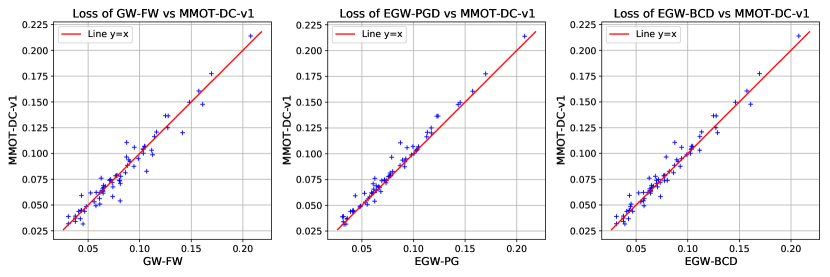
Figure 5: Scatter plots of MMOT-DC-v1 versus other solvers. In all three plots, the points tend to concentrate around the line $y=x$, which indicates the comparable performance of MMOT-DC-v1. On the other hand, the top-right plot shows the clear superiority of EGW-PGD.

MMOT-DC	MMOT-DC-v1
0.0822 ($\pm$ 0.0364)	0.0820 ($\pm$ 0.0361)

Table 2: Average and standard deviation of COOT loss of MMOT-DC and MMOT-DC-v1. The performance of the two algorithms is very similar.

References

- Agueh and Carlier [2011] Martial Agueh and Guillaume Carlier. Barycenters in the Wasserstein Space. SIAM Journal on Mathematical Analysis, 43:904–924, 2011.
- Benamou et al. [2014] Jean-David Benamou, Guillaume Carlier, Marco Cuturi, Luca Nenna, and Gabriel Peyré. Iterative Bregman Projections for Regularized Transportation Problems. SIAM Journal on Scientific Computing, 37:1111–1138, 2014.
- Birkhoff [1946] George David Birkhoff. Tres observaciones sobre el algebra lineal. Universidad Nacional de Tucuman, Revista, 5:147–150, 1946.
- Borgwardt et al. [2006] Karsten M. Borgwardt, Arthur Gretton, Malte J. Rasch, Hans-Peter Kriegel, Bernhard Schölkopf, and Alex J. Smola. Integrating structured biological data by Kernel Maximum Mean Discrepancy. Bioinformatics, 22(14):49–57, 7 2006.
- Cao et al. [2019] Jiezhang Cao, Langyuan Mo, Yifan Zhang, Kui Jia, Chunhua Shen, and Mingkui Tan. Multi-marginal Wasserstein GAN. Advances in Neural Information Processing Systems, pages 1774–1784, 2019.
- Cohen and Rothblum [1993] Joel E. Cohen and Uriel G. Rothblum. Nonnegative ranks, decompositions, and factorizations of nonnegative matrices. Linear Algebra and its Applications, 190:149–168, 1993.
- Cohen et al. [2021] Samuel Cohen, K. S. Sesh Kumar, and Marc Peter Deisenroth. Sliced multi-marginal optimal transport. ICML, 2021.
- Cuturi [2013] Marco Cuturi. Sinkhorn Distances: Lightspeed Computation of Optimal Transport. Advances in Neural Information Processing Systems, pages 2292–2300, 2013.
- Feydy et al. [2019] Jean Feydy, Thibault Séjourné, François-Xavier Vialard, Shun ichi Amari, Alain Trouvé, and Gabriel Peyré. Interpolating between Optimal Transport and MMD using Sinkhorn Divergences. Proceedings of the 22nd International Conference on Artificial Intelligence and Statistics (AISTATS), 2019.
- Flamary et al. [2021] Rémi Flamary, Nicolas Courty, Alexandre Gramfort, Mokhtar Z. Alaya, Aurélie Boisbunon, Stanislas Chambon, Laetitia Chapel, Adrien Corenflos, Kilian Fatras, Nemo Fournier, Léo Gautheron, Nathalie T.H. Gayraud, Hicham Janati, Alain Rakotomamonjy, Ievgen Redko, Antoine Rolet, Antony Schutz, Vivien Seguy, Danica J. Sutherland, Romain Tavenard, Alexander Tong, and Titouan Vayer. Pot: Python optimal transport. Journal of Machine Learning Research, 22(78):1–8, 2021. URL http://jmlr.org/papers/v22/20-451.html.
- Forrow et al. [2019] Aden Forrow, Jan-Christian Hütter, Mor Nitzan, Philippe Rigollet, Geoffrey Schiebinger, and Jonathan Weed. Statistical Optimal Transport via Factored Couplings. The 22nd International Conference on Artificial Intelligence and Statistics, pages 2454–2465, 2019.
- Frank and Wolfe [1956] Marguerite Frank and Philip Wolfe. An algorithm for quadratic programming. Naval Research Logistics Quarterly, 3(1-2):95–110, 1956.
- Gangbo and Swiech [1998] Wilfrid Gangbo and Andrzej Swiech. Optimal maps for the multidimensional Monge-Kantorovich problem. Communications on Pure and Applied Mathematics, 51:23–45, 1998.
- Genevay et al. [2019] Aude Genevay, Lénaic Chizat, Francis Bach, Marco Cuturi, and Gabriel Peyré. Sample complexity of sinkhorn divergences. Proceedings of the Twenty-Second International Conference on Artificial Intelligence and Statistics, 89:1574–1583, 2019.
- Haasler et al. [2020] Isabel Haasler, Rahul Singh, Qinsheng Zhang, Johan Karlsson, and Yongxin Chen. Multi-marginal optimal transport and probabilistic graphical models. arXiv preprint arXiv:2006.14113, 2020.
- He et al. [2019] Zhenliang He, Wangmeng Zuo, Meina Kan, Shiguang Shan, and Xilin Chen. Attgan: Facial attribute editing by only changing what you want. IEEE Trans. Image Process., 28(11):5464–5478, 2019.
- Hui et al. [2018] Le Hui, Xiang Li, Jiaxin Chen, Hongliang He, and Jian Yang. Unsupervised multi-domain image translation with domain-specific encoders/decoders. In 24th International Conference on Pattern Recognition, ICPR 2018, Beijing, China, August 20-24, 2018, pages 2044–2049. IEEE Computer Society, 2018.
- Janati et al. [2020] Hicham Janati, Marco Cuturi, and Alexandre Gramfort. Spatio-temporal alignments: Optimal transport through space and time. In Proceedings of the Twenty Third International Conference on Artificial Intelligence and Statistics, volume 108 of Proceedings of Machine Learning Research, pages 1695–1704. PMLR, 26-28 Aug 2020.
- Kellerer [1984] Hans G Kellerer. Duality theorems for marginal problems. Zeitschrift für Wahrscheinlichkeitstheorie und verwandte Gebiete, 67:399–432, 1984.
- Lin et al. [2021] Chi-Heng Lin, Mehdi Azabou, and Eva Dyer. Making transport more robust and interpretable by moving data through a small number of anchor points. Proceedings of the 38th International Conference on Machine Learning, 139:6631–6641, 2021.
- Mi and Bento [2020] Liang Mi and José Bento. Multi-marginal optimal transport defines a generalized metric. CoRR, abs/2001.11114, 2020.
- Mémoli [2011] Facundo Mémoli. Gromov-Wasserstein distances and the metric approach to object matching. Foundations of Computational Mathematics, pages 1–71, 2011.
- Peyré et al. [2016] Gabriel Peyré, Marco Cuturi, and Justin Solomon. Gromov-Wasserstein Averaging of Kernel and Distance Matrices. International Conference on Machine Learning, 48, 2016.
- Pham and Bernoussi [1986] Tao Dinh Pham and Souad El Bernoussi. Algorithms for Solving a Class of Nonconvex Optimization Problems. Methods of Subgradients. North-Holland Mathematics Studies, 129:249–271, 1986.
- Pham and Le [1997] Tao Dinh Pham and An Hoai Thi Le. Convex analysis approach to D.C. programming: Theory, Algorithm and Applications. Acta Mathematica Vietnamica, 22:289–355, 1997.
- Ramdas et al. [2017] Aaditya Ramdas, Nicolás García Trillos, and Marco Cuturi. On Wasserstein Two-Sample Testing and Related Families of Nonparametric Tests. Entropy, 19, 2017.
- Redko et al. [2020] Ievgen Redko, Titouan Vayer, Rémi Flamary, and Nicolas Courty. CO-Optimal Transport. Advances in Neural Information Processing Systems, 2020.
- Scetbon et al. [2021] Meyer Scetbon, Marco Cuturi, and Gabriel Peyré. Low-Rank Sinkhorn Factorization. Proceedings of the 38th International Conference on Machine Learning, 139:9344–9354, 2021.
- Schmitzer [2019] Bernhard Schmitzer. Stabilized Sparse Scaling Algorithms for Entropy Regularized Transport Problems. SIAM Journal on Scientific Computing, 41:1443–1481, 2019.
- Schoenberg [1938] I. J. Schoenberg. Metric Spaces and Positive Definite Functions. Transactions of the American Mathematical Society, 44:522–536, 11 1938.
- Séjourné et al. [2020] Thibault Séjourné, François-Xavier Vialard, and Gabriel Peyré. The Unbalanced Gromov Wasserstein Distance: Conic Formulation and Relaxation. arXiv preprint arXiv:2009.04266, 2020.
- Vo [2015] Thanh Xuan Vo. Learning with sparsity and uncertainty by Difference of Convex functions optimization. PhD thesis, Université de Lorraine, 2015.