Abstract

Multi-marginal optimal transport (MOT) is a generalization of optimal transport to multiple marginals. Optimal transport has evolved into an important tool in many machine learning applications, and its multi-marginal extension opens up for addressing new challenges in the field of machine learning. However, the usage of MOT has been largely impeded by its computational complexity which scales exponentially in the number of marginals. Fortunately, in many applications, such as barycenter or interpolation problems, the cost function adheres to structures, which has recently been exploited for developing efficient computational methods. In this work we derive computational bounds for these methods. In particular, with $m$ marginal distributions supported on $n$ points, we provide a $\mathcal{\tilde{O}}(d(\mathcal{T})mn^{w(G)+1}\epsilon^{-2})$ bound for a $\epsilon$-accuracy when the problem is associated with a graph that can be factored as a junction tree with diameter $d(\mathcal{T})$ and tree-width $w(G)$. For the special case of the Wasserstein barycenter problem, which corresponds to a star-shaped tree, our bound is in alignment with the existing complexity bound for it.

1 Introduction

The history of optimal transport can be traced back to the 18-th century when the French mathematician Monge introduced this tool for his engineering projects. In optimal transport problems one seeks an optimal strategy to move resources from an initial distribution to a target one. This theory has initially had a tremendous impact to fields such as economics and logistics. During the last decades, with new efficient computational methods (Villani, 2009; Cuturi, 2013) and more available computational power, optimal transport theory has also been used for addressing a broad class of problems both within the machine learning community (Peyré et al., 2019; Solomon et al., 2014, 2015; Arjovsky et al., 2017), but also in related fields such as imaging (Haker et al., 2004) and systems and control (Chen et al., 2016).

Multi-marginal optimal transport (MOT) is a natural extension of standard optimal transport to scenarios with more than two marginal distributions. In the discrete setting, the objective of MOT is to find an optimal coupling between $m$ marginals $\mu_{1},\dots,\mu_{m}\in\mathbb{R}_{+}^{n}$ over $X$, where $X$ is a discrete space with support in $n$ points. A $m$-mode tensor ${\bf B}\in\mathbb{R}_{+}^{n^{m}}$ is a feasible transport plan if it satisfies the assigned marginals, $P_{k}({\bf B})=\mu_{k}$, where

$$[P_{k}({\bf B})](x_{k})=\sum_{{\bf x}\setminus x_{k}}{\bf B}({\bf x}),\quad\text{for all }x_{k}\in X,$$ (1)

where ${\bf x}=(x_{1},\dots,x_{m})\in X^{m}$. In this paper we consider a version of this problem where the marginals are typically only imposed on a subset of the transport tensors nodes, and we denote this subset of indices by $\Gamma\subset\{1,\dots,m\}$. The set of feasible transport plans consistent with these marginals $\{\mu_{k}\}_{k\in\Gamma}$ is then

$${\Pi_{\Gamma}^{m}((\mu_{k})_{k\in\Gamma})}=\{{\bf B}\in\mathbb{R}^{n^{m}}:P_{k}({\bf B})=\mu_{k},\forall k\in\Gamma\}.$$ (2)

Given a non-negative cost tensor ${\bf C}\in\mathbb{R}^{n^{m}}_{+}$, where ${\bf C}({\bf x})$ denotes the cost associated with a unit mass on the tuple ${\bf x}$, the multi-marginal optimal transport problem reads

$$\min_{{\bf B}\in{\Pi_{\Gamma}^{m}((\mu_{k})_{k\in\Gamma})}}\langle{\bf C},{\bf B}\rangle.$$ (3)

The MOT problem is a linear program, thus, in principle, the simplex algorithm can be used to solve it exactly. The complexity however explodes quickly as the problem size increases. In practice, the MOT is solved approximately instead. The goal of these approximation algorithms is to find $\widehat{\bf B}\in{\Pi_{\Gamma}^{m}((\mu_{k})_{k\in\Gamma})}$ such that $\langle{\bf C},\widehat{\bf B}\rangle$ is an $\epsilon$-approximation of the MOT problem (3). That is, $\widehat{\bf B}$ is an approximation of the transport tensor and satisfies

$$\langle{\bf C},\widehat{\bf B}\rangle\leq\min_{{\bf B}\in{\Pi_{\Gamma}^{m}((\mu_{k})_{k\in\Gamma})}}\langle{\bf C},{\bf B}\rangle+\epsilon.$$ (4)

A popular method to approximately solve the MOT problem (3) is to solve an entropic regularized version of it where an entropy barrier term is added to the objective. This regularized problem can be solved by the renowned Sinkhorn iterations (Deming & Stephan, 1940; Cuturi, 2013).

Related work:

A fundamental question in the study of MOT algorithms is understanding their complexities, and several complexity bounds have been derived over the last few years for various MOT algorithms (Lin et al., 2019; Altschuler & Boix-Adsera, 2020; Carlier, 2021). The best known complexity bound for the general multi-marginal Sinkhorn iterations is$\mathcal{\tilde{O}}(\frac{m^{3}n^{m}}{\epsilon^{2}})$ (Lin et al., 2019) with greedy updates, which scales exponentially in the number of marginals $m$. This is not surprising as the size of the variable ${\bf B}$ grows exponentially. This complexity bound can be improved by exploiting the structure of the cost tensor ${\bf C}$. A well-known example is the Wasserstein barycenter problem where the cost can be decomposed into pairwise costs between the marginals and the barycenter. Kroshnin et al. (2019) shows that the iterative scaling algorithm finds an $\epsilon$-approximate solution to the barycenter between $L$ distributions in $\mathcal{\tilde{O}}(\frac{Ln^{2}}{\epsilon^{2}})$ operations. A more general class of costs where better computation complexity can be achieved is associated with the tree structure (see Section 2). Such structures appear in various applications, such as barycenter problems (Lin et al., 2020; Kroshnin et al., 2019), interpolation problems (Solomon et al., 2015), and estimation problems (Elvander et al., 2020). It was shown in Haasler et al. (2021c) that a complexity bound for MOT problems with tree-structured cost (including the barycenter problem as a special case) is $\mathcal{\tilde{O}}(\frac{m^{4}n^{2}}{\epsilon^{2}})$, where $m$ denotes the number of marginals. Many other MOT problems are structured according to graphs that contain cycles, e.g., in the generalized Euler flow problem (Benamou et al., 2015), control applications (Haasler et al., 2020), and multi-species problems (Haasler et al., 2021b). In Altschuler & Boix-Adsera (2020), it was shown that the complexity for MOT with general graph-structured cost scales polynomially as the number of marginals increases, as long as the tree-width of the graph is properly bounded, but they do not provide explicit dependencies on the parameters. Note that some other structures of the cost tensors such as the low rank property can be leveraged (Altschuler & Boix-Adsera, 2020), but these are very different to the graphical structure considered in this work.

Our contribution:

The purpose of this work is to provide a tighter complexity bound for solving the MOT problem with general graph-structured costs. Tree-structured optimal transport problems are often formulated as a sum of bi-marginal optimal transport problem. The numerical scheme is often based on regularizing each of the bi-marginal problems locally in previous work. However, if the underlying graph structure contains cycles, there is no such representation of the problem. In this work we suggest to use a regularization on the MOT tensor similar to the one suggested in Carlier (2021). This regularization also simplifies the complexity analysis (see Remark 1). For the cases where the MOT problem is structured according to a tree, i.e., the graph does not contain any cycles, we show that an $\epsilon$-approximation of the solution can be found within $\mathcal{\tilde{O}}(\bar{d}(G)mn^{2}\epsilon^{-2})$ operations, where $\bar{d}(G)$ denotes the average distance between two leaves of the tree. This improves on the previous result $\mathcal{\tilde{O}}(m^{4}n^{2}\epsilon^{-2})$ for tree-structured MOT in Haasler et al. (2021c). Especially for the barycenter problem, which corresponds to the special case of a star-shaped graph, this matches the best known bound when no further acceleration of the method is applied. The framework in this paper also treats a class of MOT problems that is much larger than what can be described by bi-marginal OT problems. In the case of a general graph $G$, the complexity is $\mathcal{\tilde{O}}\left(\bar{d}(\mathcal{T})mn^{w(G)+1}\epsilon^{-2}\right)$, where $\mathcal{T}$ is a minimal junction tree over the graph $G$, and $w(G)$ is the tree-width of $G$. The best-known complexity bounds for optimal transport without acceleration are summarized in Table 1. There are accelerated versions of the Sinkhorn algorithm, see, e.g., Lin et al. (2019); Kroshnin et al. (2019) that can improve the dependence with respect to $\epsilon$ from $\epsilon^{-2}$ to $\epsilon^{-1}$. Note that these accelerations cannot improve the dependence over $m$ or $n$. Since the algorithm studied in this work is not accelerated, we compare the complexity bounds only to algorithms with no acceleration.

Table 1: Best-known complexity bounds for optimal transport without acceleration

Problem	Complexity	Paper
Bi-marginal optimal transport	$\mathcal{\tilde{O}}(n^{2}\epsilon^{-2})$	Dvurechensky et al. (2018)
Barycenter optimal transport	$\mathcal{\tilde{O}}(mn^{2}\epsilon^{-2})$	Kroshnin et al. (2019)
General MOT	$\mathcal{\tilde{O}}(m^{3}n^{m}\epsilon^{-2})$	Lin et al. (2019)
Tree-structured MOT	$\mathcal{\tilde{O}}(m^{4}n^{2}\epsilon^{-2})$	Haasler et al. (2021c)
Tree-structured MOT	$\mathcal{\tilde{O}}(\bar{d}(G)mn^{2}\epsilon^{-2})$	Ours
balanced Graph-structured MOT	$\mathcal{\tilde{O}}(\bar{d}(\mathcal{T})mn^{w(G)+1}\epsilon^{-2})$	Ours

Figure 1: Graph associated with a barycenter problem (5), where $L=5$.

Notation:

For a matrix $C\in\mathbb{R}^{n\times n}$, we denote $\|C\|_{\infty}$ its largest element. We denote a graph as the tuple $G=(V,E)$, where $V$ is the set of vertices, and $E$ is the set of edges. For a vertex $k\in V$, we denote the set of neighbouring vertices by $N(k)\subset V$. Let $\mathbf{1}_{d}$ denote the all-ones vector/matrix/tensor in ${\mathbb{R}}^{d}$, and let $\exp(\cdot),\log(\cdot),\odot$, and $./$ denote the element-wise exponential, logarithm, multiplication, and division of tensors, respectively. The $p(m,n,\epsilon)=\mathcal{\tilde{O}}(q(m,n,\epsilon))$ notation absorbs polylogarithmic factors related to $n$, i.e., there exist positive constants $c_{2},c_{3}$ such that $p(m,n,\epsilon)\leq c_{2}q(m,n,\epsilon)(\log n)^{c_{3}}$.

2 Graph-structured MOT

In this paper we consider MOT problems with a cost that decouples according to a graph. Such structures appear in many applications, for instance in barycenter problems (Lin et al., 2020; Kroshnin et al., 2019), interpolation problems (Solomon et al., 2015), and estimation problems (Elvander et al., 2020; Singh et al., 2020). In fact, one of the very first studies of MOT, on the generalized Euler-flow problem, has a graph-structured cost (Brenier, 1989; Benamou et al., 2015).

Example 1.

(Fixed-support Wasserstein Barycenter).

A special case of a graph-structured optimal transport problem is the fixed support barycenter problem with uniform weights

$$\min_{\mu\in\mathbb{R}^{n}}\sum_{\ell=1}^{L}\frac{1}{L}W(\mu,\mu_{\ell}),~{}\text{ with }~{}W(\mu,\nu)=\inf_{B\in\Pi(\mu,\nu)}\langle C,B\rangle,$$ (5)

where $\Pi(\mu,\nu)=\Pi^{2}_{\{1,2\}}(\mu,\nu)$ denotes the standard set of feasible transport plans for two marginals. The underlying structure can be described by a star-graph as illustrated in Figure 1. Problem (5) can be written as the multi-marginal problem (3), where the cost tensor ${\bf C}\in\mathbb{R}^{n^{L+1}}$ is defined as

$${\bf C}(x_{1},\dots,x_{L},x_{L+1})=\sum_{\ell=1}^{L}\frac{1}{L}C(x_{L+1},x_{\ell}),$$ (6)

and constraints are given on the set $\Gamma=\{1,\dots,\ell\}$.

Similar to Example 1, we can define a MOT problem that is structured according to any graph $G=(V,E)$. Therefore, we associate each vertex in $V$ with a marginal of the transport plan ${\bf B}$, and each edge in $E$ with a pair-wise cost. That is, for the interaction between vertices $k_{1}$ and $k_{2}$ we define a cost matrix $C^{(k_{1},k_{2})}$, and we let $E$ be the set of all these pair-wise interactions. Then the graph-structured cost tensor is defined by

$${\bf C}(x_{1},\dots,x_{m})=\sum_{(k_{1},k_{2})\in E}C^{(k_{1},k_{2})}(x_{k_{1}},x_{k_{2}}).$$ (7)

Problem (3) with a cost tensor of the form (7) is called a graph-structured MOT problem (Haasler et al., 2021a, c).

Many graph-structured optimal transport problems, for instance interpolation and barycenter problems, are naturally described by tree graphs, i.e., graphs that do not contain any cycles. Moreover, any graph can be converted into a tree using the junction tree technique (Koller & Friedman, 2009), and we will use this representation to derive complexity bounds for general graph-structured MOT problems. It should be noted that in the case of a tree-structured MOT problem we can without loss of generality consider the case, where $\Gamma$ is the set of leaves (Haasler et al., 2021a, Proposition 3.4).

3 Sinkhorn belief propagation algorithm

In practical applications the MOT problem is often prohibitively large for standard linear programming solvers, and one therefore has to resort to numerical methods to obtain an appropriate solution. A well-known approach, based on the seminal work by Cuturi (2013), is to regularize the objective in (3) with an entropic barrier term (Benamou et al., 2015). In particular, we introduce the barrier term

$$H({\bf B}\mid{\bf M})=\langle{\bf B},\log({\bf B})-\log({\bf M})-\mathbf{1}_{n^{m}}\rangle,$$ (8)

where

$${\bf M}(x_{1},x_{2},\ldots,x_{m})=\prod_{k\in\Gamma}\mu_{k}(x_{k}).$$ (9)

The regularized MOT problem reads then

$$\min_{{\bf B}\in{\Pi_{\Gamma}^{m}((\mu_{k})_{k\in\Gamma})}}\langle{\bf C},{\bf B}\rangle+\eta H({\bf B}\mid{\bf M}),$$ (10)

where $\eta>0$ is a small regularization parameter.

Remark 1.

Note that our choice of entropy regularizer is slightly different from the standard one $\langle{\bf B},\log({\bf B})-\mathbf{1}_{n^{m}}\rangle$ often used for the Sinkhorn algorithm. The extra term $-\langle{\bf B},\log({\bf M})\rangle$ turns out to simplify the approximation procedure (there is no need to alter the marginal distributions first to increase the minimum value of their elements as in Dvurechensky et al. (2018); Lin et al. (2019)) and the complexity analysis (see, e.g., Lemma 1).

The optimal solution of the regularized multi-marginal optimal transport problem (10) can be compactly expressed in terms of the optimal variables of the dual problem. More precisely, the optimal transport tensor is of the form

$$[{\bf B}(\Lambda)](x_{1},\dots,x_{m})= \exp\left(-{\bf C}(x_{1},\dots,x_{m})/\eta\right)$$

$$\cdot\prod_{k\in\Gamma}\Big{(}\exp\!\Big{(}\frac{\lambda_{k}(x_{k})}{\eta}\Big{)}\mu_{k}(x_{k})\Big{)},$$ (11)

where $\Lambda=\{\lambda_{k}\}_{k\in\Gamma}$ is the optimal solution of the dual of (10), which is given by (cf. Haasler et al. (2021a))

$$\min_{\Lambda}\psi(\Lambda):=\eta P({\bf B}(\Lambda))-\sum_{k\in\Gamma}\mu_{k}^{\text{T}}\lambda_{k}.$$ (12)

Here, $P({\bf B})=\sum_{{\bf x}}{\bf B}({\bf x})\in\mathbb{R}$ is the projection over all marginals of ${\bf B}$, i.e., the sum over all elements.

The optimal solution to (12) can be efficiently found by the renowned Sinkhorn iterations (Benamou et al., 2015; Haasler et al., 2021c). In particular, the multi-marginal Sinkhorn algorithm is to find the scaled variables $u_{k}=\exp(\lambda_{k}/\eta)$, for $k\in\Gamma$, by iteratively updating them according to

$$u_{k}^{(t+1)}\leftarrow u_{k}^{(t)}\odot\mu_{k}./P_{k}({\bf B}(\Lambda^{(t)})).$$ (13)

There are several approaches to perform these updates: At each iteration, the next marginal $k\in\Gamma$ to be updated can be picked in a random, cyclic, or greedy fashion (Benamou et al., 2015; Lin et al., 2019). In this paper we discuss the random updating rule. The greedy update requires more operations for each iteration as all the projections for $k\in\Gamma$ are needed for an update. The traditional cyclic update introduces strong couplings between updates which makes the complexity analysis much more challenging.

For general MOT, computing the projections $P_{k}({\bf B}(\Lambda^{(t)}))$ requires $\mathcal{O}(n^{m})$ operations, which creates a large computational burden. However, in case the MOT problem has a tree-structure, the projections $P_{k}({\bf B}(\Lambda^{(t)}))$ can be computed by a message-passing algorithm that utilizes the belief propagation algorithm (Yedidia et al., 2003), as described in Haasler et al. (2021c, a). This requires only matrix-vector multiplications of size $n$. In particular, the projections are of the form

$$[P_{k}({\bf B}(\Lambda^{(t)}))](x_{k})=$$ (14)

$$\begin{dcases}u_{k}^{(t)}(x_{k})\mu_{k}(x_{k})m_{{\color[rgb]{0,0,0}{\ell_{k}}}\to k}(x_{k}),&\quad\text{ if }k\in\Gamma\\ \prod_{\ell\in N(k)}m_{\ell\to k}(x_{k}),&\quad\text{ if }k\notin\Gamma,\end{dcases}$$ (15)

where the messages are computed as

$$m_{\ell\to k}(x_{k})=$$ (16)

$$\begin{dcases}\sum_{x_{\ell}}K^{(k,\ell)}(x_{k},x_{\ell})\prod_{j\in N(\ell)\setminus k}m_{j\to\ell}(x_{\ell}),\quad\text{ if }\ell\notin\Gamma\\ \sum_{x_{\ell}}K^{(k,\ell)}(x_{k},x_{\ell})u_{\ell}^{(t)}(x_{\ell})\mu_{\ell}(x_{\ell}),\quad\text{ if }\ell\in\Gamma,\end{dcases}$$ (17)

where $K^{(k,\ell)}(x_{k},x_{\ell})=\exp(-C^{(k,\ell)}(x_{k},x_{\ell})/\eta)$.

Since we can without loss of generality assume that $\Gamma$ is the set of leaves of the tree, each vertex $k\in\Gamma$ has a unique neighbour $\ell_{k}\in N(k)$. The Sinkhorn iterations (13) with the projections (15) thus read

$$u_{k}^{(t+1)}(x_{k})\leftarrow(m_{\ell_{k}\to k}(x_{k}))^{-1}.$$ (18)

Note that when we update the scaling vectors $u_{k^{(t)}}^{(t)}$ and in the previous iteration updated $u_{k^{(t-1)}}^{(t-1)}$ it is only required to recompute the messages between $k^{(t-1)}$ and $k^{(t)}$ (Haasler et al., 2021c; Singh et al., 2020). The Sinkhorn method is summarized in Algorithm 1. Here, we apply a random updating scheme, where the next scaling vector to be updated is picked from a uniform distribution of the remaining scaling vectors, except the previous one. Other common update rules for the Sinkhorn iterations, such as cyclic or greedy updates, can be obtained by simply changing the selection of $k^{(t)}$ in Algorithm 1.

Algorithm 1 SINKHORN_BP($\epsilon^{\prime},\{\mu_{k}\}_{k\in\Gamma},{\bf C},\eta$)

Initialization: $u_{k}^{(0)}=\mathbf{1}\in{\mathbb{R}}^{n}$, for $k\in\Gamma$;  $t=1$;  $k^{(0)}\in\Gamma$

while  $\sum_{k\in\Gamma}\|P_{k}({\bf B}(\Lambda^{(t)}))-\mu_{k}\|_{1}\geq\epsilon^{\prime}$ do

   1. Randomly pick $k^{(t)}\in\Gamma\setminus k^{(t-1)}$

   2. Update messages $m_{k_{1}\to k_{2}}$ according to (17) on the path from $k^{(t-1)}$ to $k^{(t)}$

   3. Update $u_{k}^{(t+1)}(x_{k})$ to be

$$\begin{cases}(m_{\ell_{k}\to k}(x_{k}))^{-1},&\text{ for }k=k^{(t)},\text{ and }\ell_{k}\in N(k),\\ u_{k}^{(t)}(x_{k}),&\text{ for }k\in\Gamma\setminus k^{(t)},\end{cases}$$

   4. $t\leftarrow t+1$

end while

Output: $u_{k}^{(t+1)}$, $k\in\Gamma$

From the scaling vectors $\{u_{k}\}_{k\in\Gamma}$ that are returned from Algorithm 1 we can construct the transport tensor $\widetilde{\bf B}$ as in (3). However, this tensor is not guaranteed to lie in the feasible set ${\Pi_{\Gamma}^{m}((\mu_{k})_{k\in\Gamma})}$, and thus a rounding step is needed. This is based on the rounding for bi-marginal optimal transport in (Altschuler et al., 2017, Algorithm 2), and is stated in Algorithm 2. Note that a transport tensor that solves a graph-structured MOT problem (3) or (10) is fully determined by the projections $P_{k_{1},k_{2}}({\bf B})$ on the edges $(k_{1},k_{2})\in E$ (Koller & Friedman, 2009), which are given by

$$[P_{k_{1},k_{2}}({\bf B})](x_{k_{1}},x_{k_{2}})=\sum_{{\bf x}\setminus\{x_{k_{1}},x_{k_{2}}\}}{\bf B}({\bf x}).$$ (19)

By slight abuse of notation, we let ${\bf B}((B_{k_{1},k_{2}})_{(k_{1},k_{2})\in E})$ denote this tensor that decouples according to the tree structure $G$ and satisfies the projections $[P_{k_{1},k_{2}}({\bf B})]=B_{k_{1},k_{2}}$ for $(k_{1},k_{2})\in E$ (Koller & Friedman, 2009). Note that the projections (19) can be cheaply computed from the scaling vectors $\{u_{k}\}_{k\in\Gamma}$ as described in (Haasler et al., 2021c, Theorem 4).

Algorithm 2 ROUND $({\bf B},\{\mu_{k}\}_{k\in\Gamma})$

Initialization: ${\bf B}_{k,\ell_{k}}=P_{k,\ell_{k}}({\bf B})\in{\mathbb{R}}^{n\times n}$ for all $k\in\Gamma$ and each $\ell_{k}\in N(k)$

for $k\in\Gamma$ do

   Input $\left({\bf B}_{k,\ell_{k}};P_{\ell_{k}}({\bf B}),\mu_{k}\right)$ into (Altschuler et al., 2017, Algorithm 2) and get $\widehat{{\bf B}}_{k,\ell_{k}}$ such that $\widehat{{\bf B}}_{k,\ell_{k}}\in\Pi(P_{\ell_{k}}({\bf B}),\mu_{k})$

end for

Output: $\widehat{\bf B}=\{\widehat{\bf B}_{k,\ell_{k}};k\in\Gamma\}\cup\{P_{k_{1},k_{2}}({\bf B});(k_{1},k_{2})\in E,k_{1},k_{2}\notin\Gamma\}$

The full method for finding an $\epsilon$-approximate solution to a tree-structured MOT problem is summarized in Algorithm 3.

Algorithm 3 $\epsilon$-approximation of tree-structured MOT

$\eta\leftarrow\frac{\epsilon}{2m\log(n)}$;   $\epsilon^{\prime}\leftarrow\frac{\epsilon}{8{R_{C}^{\Gamma}}}$ .

$\{u_{k}\}_{k\in\Gamma}\leftarrow\text{SINKHORN\_BP}(\epsilon^{\prime},\{\mu_{k}\}_{k\in\Gamma},{\bf C},\eta)$. (Algorithm 1)

Construct $\widetilde{\bf B}(B_{k_{1},k_{2},(k_{1},k_{2})\in E})$ from $\{u_{k}\}_{k\in\Gamma}$

$\widehat{\bf B}\leftarrow\text{ROUND}(\widetilde{{\bf B}},\{\mu_{k}\}_{k\in\Gamma})$. (Algorithm 2)

Output: $\widehat{{\bf B}}$

4 Tree structured MOT analysis

In this section, we present a complexity bound for the Sinkhorn belief propagation algorithm for solving MOT problems with tree-structured costs. We first provide a few technical lemmas that will be used in the proof. The proofs of all the supporting lemmas are given in the supplementary material. The first result provides bounds for the scaling vector iterates.

Lemma 1.

Let $\lambda_{k}=\eta\log(u_{k})$, where $u_{k}$ are generated by Algorithm 1. Let $\Lambda^{*}=\{\lambda_{k}^{*}\}_{k\in\Gamma}$ be a solution of (12). Then for each $k\in\Gamma$ it holds

$$\max_{x_{k}}\lambda_{k}(x_{k})-\min_{x_{k}}\lambda_{k}(x_{k})\leq R_{C}^{k},$$

$$\max_{x_{k}}\lambda_{k}^{*}(x_{k})-\min_{x_{k}}\lambda_{k}^{*}(x_{k})\leq R_{C}^{k},$$

where

$$R_{C}^{k}:=\|C^{(k,\ell_{k})}\|_{\infty},$$

and where $\ell_{k}\in N(k)$ is the (unique) neighbour of $k$.

The following Lemma relates the error in the dual objective value to the stopping criterion of Algorithm 1.

Lemma 2.

Let $\Lambda=\{\lambda_{k}\}_{k\in\Gamma}$, where $\lambda_{k}=\eta\log(u_{k})$ and $u_{k}$ are generated by Algorithm 1, and let $\Lambda^{*}=\{\lambda_{k}^{*}\}_{k\in\Gamma}$ be a solution to (12). Then it holds

$$\psi(\Lambda)-\psi(\Lambda^{*})\leq{R_{C}^{\Gamma}}\sum_{k\in\Gamma}\|P_{k}({\bf B}(\Lambda))-\mu_{k}\|_{1},$$ (20)

with ${R_{C}^{\Gamma}}=\max_{k\in\Gamma}R_{C}^{k}$, where $R_{C}^{k}$ is defined as in Lemma 1.

The increment between two sequential Sinkhorn iterates is related to the stopping criterion of Algorithm 1 as described in the following.

Lemma 3.

For any $\Lambda^{(t)}$, let $\Lambda^{(t+1)}$ be the next iterate of the algorithm in (13).

$${\mathbb{E}}\left[\psi(\Lambda^{(t)})-\psi(\Lambda^{(t+1)})\right]\geq\frac{\eta}{2|\Gamma|^{2}}\left(e_{t}\right)^{2},$$ (21)

with

$$e_{t}:=\sum_{k\in\Gamma}\|P_{k}({\bf B}(\Lambda^{(t)}))-\mu_{k}\|_{1}.$$ (22)

The expectation is over the uniform distribution of $k^{(t+1)}\in\Gamma\setminus k^{(t)}$.

We are now ready to state our first main result, which gives two probabilistic bounds on the required number of iterations in Algorithm 1.

Theorem 1.

For sufficiently small $\eta$, Algorithm 1 generates a tensor ${\bf B}(\Lambda^{(t)})$ satisfying

$$\sum_{k\in\Gamma}\|P_{k}({\bf B}(\Lambda^{(t)}))-\mu_{k}\|_{1}\leq\epsilon^{\prime},$$

within $\tau$ iterations, where

$${\mathbb{E}}[\tau]\leq\frac{8|\Gamma|^{2}{R_{C}^{\Gamma}}}{\eta\epsilon^{\prime}}.$$

Moreover, for any $\delta\in(0,0.5),$ it holds that

$${\mathbb{P}}\left(\tau\leq\frac{48|\Gamma|^{2}{R_{C}^{\Gamma}}}{\eta\epsilon^{\prime}}\log\frac{1}{\delta}\right)\geq 1-{\delta}.$$

Proof sketch (see supplementary material for details).

Define the stopping time $\tau:=\min\left\{t:e_{t}\leq\epsilon^{\prime}\right\}$. Let $\{{\mathcal{F}}_{t}:=\sigma\left(\Lambda^{(1)},\ldots,\Lambda^{(t)}\right)\}_{t}$ be the natural filtration. By Lemma 2 and Lemma 3,

$${\mathbb{E}}\left[\psi(\Lambda^{(t)})-\psi(\Lambda^{(t+1)})|{\mathcal{F}}_{t},t<\tau\right]$$

$$\geq\frac{\eta}{2|\Gamma|^{2}}\left(\max\left\{\frac{\psi(\Lambda^{(t)})-\psi(\Lambda^{*})}{{R_{C}^{\Gamma}}},\epsilon^{\prime}\right\}\right)^{2},$$

Let $\tau_{1}$ be the first iteration when $\psi(\Lambda^{(t)})-\psi(\Lambda^{*})\leq{R_{C}^{\Gamma}}\epsilon^{\prime}$ and $\tau_{2}:=\tau-\tau_{1}\geq 0$. We can bound $\tau_{1}$ and $\tau_{2}$ as

$${\mathbb{E}}[\tau_{1}]\leq\frac{6|\Gamma|^{2}{R_{C}^{\Gamma}}}{\eta\epsilon^{\prime}}-1,\mbox{ and }\;{\mathbb{E}}[\tau_{2}]\leq\frac{2|\Gamma|^{2}{R_{C}^{\Gamma}}}{\eta\epsilon^{\prime}}+1.$$

Summing up the two bounds results in the bound for ${\mathbb{E}}[\tau]$. The bound in probability follows similarly.∎

Remark 2.

High probability bounds are often used in machine learning algorithms when randomness is involved. Due to the logarithmic dependence $\log(1/\delta)$ in terms of the probability $1-\delta$, the high probability bound can safely be used as a surrogate of the deterministic bound.

In order to provide the complexity on the full method in Algorithm 3 we need the following two lemmas, which deal with the rounding method in Algorithm 2.

Lemma 4.

Let ${\bf B}\in{\mathbb{R}}^{n^{m}}$, where $m\geq 3$, be a nonnegative $m$-mode tensor and $\{\mu_{k}\}_{k\in\Gamma}$ be a sequence of probability vectors, Algorithm 2 returns $\widehat{{\bf B}}$ satisfying $P_{k}({\bf B})=P_{k}(\widehat{{\bf B}})$, for $k\in\Gamma$, and $P_{k}(\widehat{{\bf B}})=\mu_{k}$, for $k\in\Gamma$. Moreover, it holds that

$$\langle{\bf C},{\bf B}\rangle-\langle{\bf C},\widehat{{\bf B}}\rangle\leq 2\sum_{k\in\Gamma}\|C^{(k,\ell_{k})}\|_{\infty}\|\mu_{k}-P_{k}({{\bf B}})\|_{1},$$

where $\ell_{k}$ is the unique neighbour of $k$, for each $k\in\Gamma$.

Lemma 5.

Let $\widetilde{{\bf B}}$ be the output of Algorithm 1, let $\widehat{{\bf B}}$ be the output of Algorithm 2 with input $(\widetilde{{\bf B}},\{\mu_{k}\})$, and let ${\bf B}^{*}$ denote the optimal solution to the unregularized MOT problem (3). Then it holds that

$${\langle}{\bf C},\widehat{{\bf B}}{\rangle}-{\langle}{\bf C},{\bf B}^{*}{\rangle}\leq \ m\eta\log(n)$$

$$+4\sum_{k\in\Gamma}\|C^{(k,\ell_{k})}\|_{\infty}\|\mu_{k}-P_{k}(\widetilde{{\bf B}})\|_{1}.$$

We now have the tools to state our new complexity bound for finding $\epsilon$-approximate solutions to tree-structured MOT problems. Denote by $d(G)$ the maximum distance of two nodes in the graph $G$.

Theorem 2.

Algorithm 3 finds an $\epsilon$-approximate solution to the tree-structured MOT problem (3) in $T$ arithmetic operations, where

$${\mathbb{E}}[T]=\mathcal{O}\left(\frac{d(G)m|\Gamma|^{2}n^{2}({R_{C}^{\Gamma}})^{2}\log(n)}{\epsilon^{2}}\right).$$

Moreover, for all $\delta\in(0,0.5)$ it holds that

$${\mathbb{P}}\left(T\leq\frac{cd(G)m|\Gamma|^{2}n^{2}({R_{C}^{\Gamma}})^{2}\log(n)\log(1/\delta)}{\epsilon^{2}}\right)\geq 1-{\delta}$$

where $c$ is a universal constant.

Proof.

With the specific choices $\eta=\frac{\epsilon}{2m\log(n)}$ and $\epsilon^{\prime}=\frac{\epsilon}{8{R_{C}^{\Gamma}}}$ we get $\langle{\bf C},{\widehat{{\bf B}}}\rangle-\langle{\bf C},{{\bf B}^{*}}\rangle\leq\epsilon$. By Theorem 1, the stopping time $\tau$ satisfies

$${\mathbb{E}}[\tau]=\frac{8|\Gamma|^{2}{R_{C}^{\Gamma}}}{\eta\epsilon^{\prime}}=\mathcal{O}\left(\frac{m|\Gamma|^{2}({R_{C}^{\Gamma}})^{2}\log(n)}{\epsilon^{2}}\right).$$

Since in each iteration of Algorithm 1 the messages between two leave nodes of the tree are updated, and each message update is of complexity $\mathcal{O}(n^{2})$, one iteration takes at most $\mathcal{O}(d(G)n^{2})$ operations. Thus, in expectation, a solution is achieved in

$$\mathcal{O}\left(\frac{d(G)n^{2}m|\Gamma|^{2}({R_{C}^{\Gamma}})^{2}\log(n)}{\epsilon^{2}}\right)$$ (23)

operations. Algorithm 2 takes $\mathcal{O}(|\Gamma|n^{2})$ (see Lemma 7 in Altschuler et al. (2017)). Hence, the bound on ${\mathbb{E}}[T]$ follows. The bound in probability follows similarly. ∎

5 Extension to general graphs

For a general graph, we cannot directly apply the belief propagation algorithm. One way to tackle this is to construct a tree factorization over the graph. A junction tree (also called tree decomposition) describes a partitioning of a graph, where several nodes are clustered together, such that the interactions between the clusters can be described by a tree. A cluster $c$ is a collection of nodes, and we write ${\bf x}_{c}=\{x_{k},k\in c\}$. Moreover, the matrices $K^{(k_{1},k_{2})}=\exp(-C^{(k_{1},k_{2})}/\eta)$, for $(k_{1},k_{2})\in E$, can be understood as pair-wise potentials. A junction tree is then defined as follows.

Definition 1.

A junction tree $\mathcal{T}=(\mathcal{C},\mathcal{E})$ over a graph $G=(V,E)$ is a tree whose nodes $c\in\mathcal{C}$ are associated with subsets ${\bf x}_{c}\subset V$, and that satisfies the following properties:

• Family preservation: For each potential $K$ there is a cluster $c$ such that $\text{domain}(K)\subset{\bf x}_{c}$.

• Running intersection: For every pair of clusters $c_{i},c_{j}\in\mathcal{C}$, every cluster on the path between $c_{i}$ and $c_{j}$ contains ${\bf x}_{c_{i}}\cap{\bf x}_{c_{j}}$.

For two adjoining clusters $c_{i}$ and $c_{j}$, we define the separation set $S_{ij}=\{v\in V:v\in c_{i}\cap c_{j}\}$.

It is often practical to find a junction tree that is as similar to a tree as possible. A measure of this is given by the following definition.

Definition 2.

For a junction tree $\mathcal{T}=(\mathcal{C},\mathcal{E})$, we define its width as

$$\text{width}(\mathcal{T})=\max_{c\in\mathcal{C}}|c|-1.$$

For a graph $G$, we define its tree-width as

$$w(G)=\min\{\text{width}(\mathcal{T})\ |\ \mathcal{T}\text{ is a junction tree for }G\}.$$

Based on this partitioning, we achieve the following complexity bound for general graph-structured MOT problems. The derivation of the modified algorithm is deferred to Section B.

Theorem 3.

Let $R=\max_{k\in\Gamma}R^{k}_{\bf C}$, where $R^{k}_{\bf C}=\|{\bf C}_{c_{\ell_{k}}}({\bf x}_{c_{\ell_{k}}})\|_{\infty}$, and $c_{\ell_{k}}$ is the neighbouring clique to $c_{k}$. A generalization of Algorithm 3 finds an $\epsilon$-approximate solution to the general graph structured MOT problem (3) in $T$ arithmetic operations, where

$${\mathbb{E}}[T]=\mathcal{O}\left(\frac{d(\mathcal{T})m|\Gamma|^{2}n^{w(G)+1}R^{2}\log(n)}{\epsilon^{2}}\right).$$ (24)

Moreover, for all $\delta\in(0,0.5)$ there exists a universal constant $c$ such that

$${\mathbb{P}}\left(T\leq\frac{cd(\mathcal{T})m|\Gamma|^{2}n^{w(G)+1}R^{2}\log(n)\log(1/\delta)}{\epsilon^{2}}\right)$$

$$\geq 1-{\delta}.$$

In Algorithm 1, the per iteration complexity is not independent of the random choice of the update, and thus not independent of the number of iterations. The results in Theorem 2 and 3 thus depend on the maximum iteration complexity, and can be improved by utilizing the expected (average) iteration complexity. Therefore, let $\bar{d}(G)$ denote the average distance between any two nodes in $\Gamma$.

Theorem 4.

A generalization of Algorithm 3 finds an $\epsilon$-approximate solution to the graph-structured MOT problem (3) in $T$ arithmetic operations, where

$${\mathbb{E}}[T]=\mathcal{O}\left(\frac{\bar{d}(\mathcal{T})m|\Gamma|^{2}n^{w(G)+1}R^{2}\log(n)}{\epsilon^{2}}\right).$$

6 Discussion of results

We consider a class of tree-structured MOT problems, which contains many MOT applications of interest.

Definition 3.

Given a sequence of tree-structured MOT problems, where the number of nodes go to infinity, we call the sequence of such problems balanced if there is a constant $c$ such that $|\Gamma|{R_{C}^{\Gamma}}\leq c\|{\bf C}\|_{\infty}$.

Many MOT problems that arise in practice are balanced, see Section C.1 for a number of examples. From Theorem 2 it follows that Algorithm 3 finds an $\epsilon$-approximate solution to balanced MOT problem (3) in $T$ operations, where

$${\mathbb{E}}[T]=\mathcal{O}\left(\frac{\bar{d}(G)mn^{2}\|{\bf C}\|_{\infty}^{2}\log(n)}{\epsilon^{2}}\right).$$ (25)

This lets us compare our result with the bound for general MOT problems in Lin et al. (2019) without acceleration, which is given by $\mathcal{O}\left(m^{3}n^{m}\|{\bf C}\|_{\infty}^{2}\log(n)\epsilon^{-2}\right)$. Moreover, when the MOT problem on the junction tree is balanced, by a similar argumentation the expectation bound in Theorem 3 can be given by

$${\mathbb{E}}[T]=\mathcal{O}\left(\frac{\bar{d}(\mathcal{T})mn^{w(G)+1}\|{\bf C}\|_{\infty}^{2}\log(n)}{\epsilon^{2}}\right).$$ (26)

In case the underlying graph is fully connected and not balanced we have $\bar{d}(\mathcal{T})=2$, $w(G)=m-1$ and $R=\|{\bf C}\|_{\infty}$ in Theorem 4. In fact, in this case our algorithm does not exploit any graph structures, and thus the complexity is the same for general cost tensors that do not decouple into pairwise terms as in (7). Thus, the complexity of Algorithm 3 for general MOT problems matches the bound for general MOT problems in Lin et al. (2019).

Consider the barycenter problem introduced in Example 1. This problem is a MOT problem (3) with underlying graph as illustrated in Figure 1. Here, $d(G)=2$, $|\Gamma|=L$, and $m=L+1$. Moreover, by (6), we have ${R_{C}^{\Gamma}}=\frac{1}{L}\|C\|_{\infty}$. Thus, Algorithm 3 is expected to return an $\epsilon-$approximate solution to problem 5 in $\mathcal{O}(Ln^{2}\|C\|_{\infty}^{2}\log(n)\epsilon^{-2})$. This coincides with the best known bound for the barycenter problem (Kroshnin et al., 2019; Lin et al., 2020) without acceleration. In fact, the argument can be extended to the case of non-uniform weights in the barycenter problem (5), see Section C.2. We also point out that the regularizer used in the Wasserstein barycenter literature is different from ours: one is pairwise regularization and one is regularization over the full tensor ${\bf B}$. For more details on this comparison, see Haasler et al. (2021a)[Section 5].

7 Experiments

We show numerical results for three types of MOT problems. We consider the barycenter problem in Example 1, which is structured according to the graph in Figure 1, and the Hidden Markov Model example in Haasler et al. (2021c, Section V.B), which is structured according to the graph in Figure 2. In particular, these two types of problems are tree-structured.

Figure 2: Graph associated with a Hidden Markov Model.

Figure 3: Graph associated with a Wasserstein least square problem.

The third example is the Wasserstein least square problem (Karimi et al., 2020), which is associated with the graph in Figure 3. Note that this is a graph with tree-width two. In all the above graphs, gray nodes correspond to fixed marginals $\{\mu_{i}\}_{k\in\Gamma}$, and white nodes are estimated in the problem.

The cost matrices $C^{(k_{1},k_{2})}$ in (7) are set to be the squared Euclidean distance. The constrained marginal distributions $\{\mu_{k}\}_{k\in\Gamma}$ are supported on a uniform grid with $n$ points between 0 and 1, where the values are generated from the log-normal distribution and normalized to sum to one. We choose the accuracy $\epsilon=0.5$ in Algorithm 3. As a comparison, we implemented a brutal force Sinkhorn method, which computes the projections $P_{k}({\bf{B}}(\Lambda^{(t)}))$ in the Sinkhorn iterates (13) by directly summing over the elements of the tensor ${\bf{B}}(\Lambda^{(t)})$ as in (1). We use a random update rule for both methods. The number of iterations of both brutal force Sinkhorn and Sinkhorn belief propagation are nearly the same. We repeat every experiment 5 times with different random seeds and report the total run time in Figure 4. The theoretical complexity bound is also presented as dashed lines. The run time of brutal force Sinkhorn grows in a higher polynomial of $n$ and grows exponentially with respect to $m$. This coincides with the general MOT bound and our bounds in Table 1. We can also tell our bound is a bit pessimistic about the dependence over $n$.

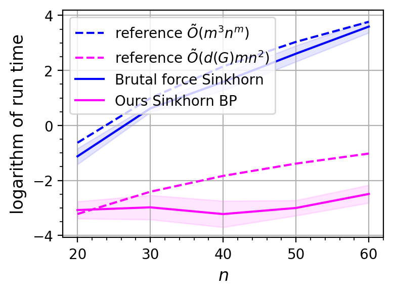
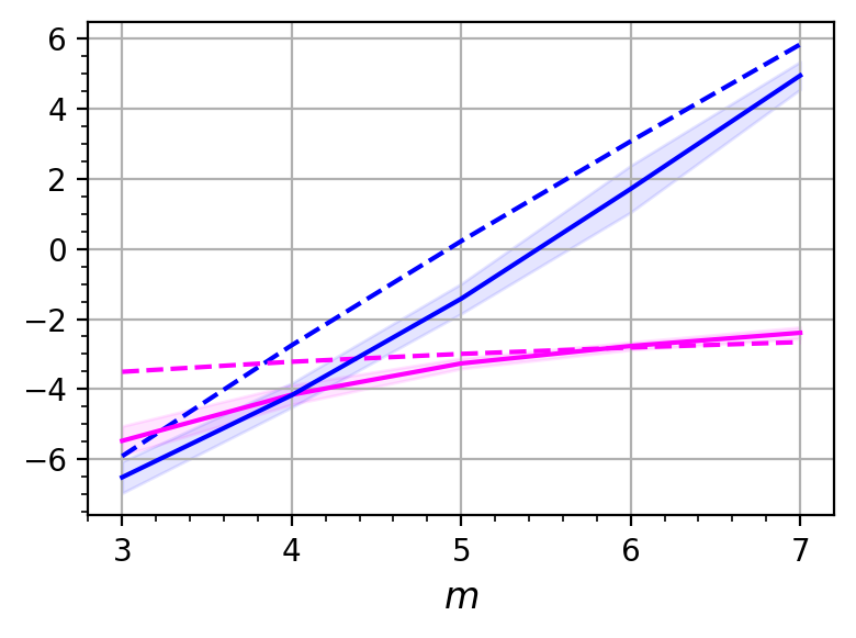
(a) Barycenter.

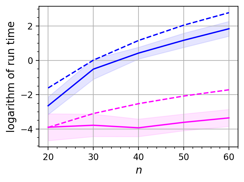
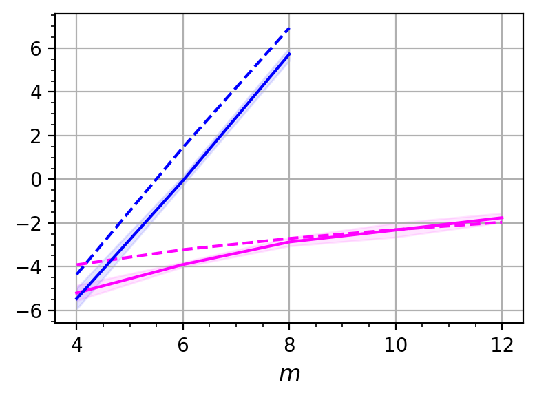
(b) Hidden Markov Model.

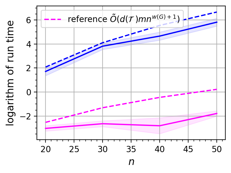
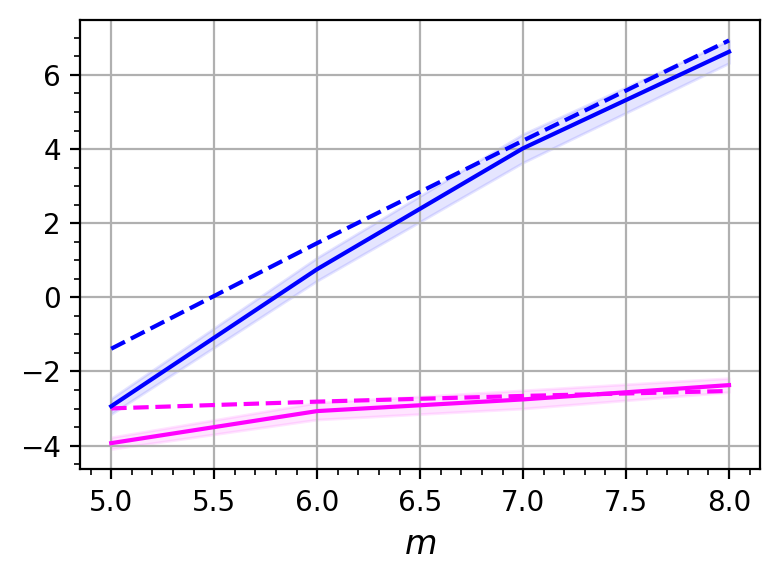
(c) Wasserstein least square.

Figure 4: Logarithm of total run time in seconds for brutal force Sinkhorn and Sinkhorn belief propagation. The left column shows the run time as a function of $n$ when $m$ is fixed ($m=4$ in (a) and (b); $m=5$ in (c)), and the right column vice versa with $n=10$.

8 Conclusion

In this work we considered a class of multi-marginal optimal transport problems where the cost functions can be decomposed according to a graph. It turns out that the computational complexity of MOT can be significantly reduced by exploiting the graphical structures. More specifically, without any structure, the complexity grows exponentially as the number of marginals increases. With graphical structure, the dependence becomes polynomial. We provide a complexity bound $\mathcal{\tilde{O}}(d(\mathcal{T})mn^{w(G)+1}\epsilon^{-2})$ for solving graph-structured MOT problems based on the Sinkhorn belief propagation algorithm (Haasler et al., 2021c; Singh et al., 2020) with the random updating rule. One limitation of the present work is that the proof techniques do not seem to be applicable to Sinkhorn iterations with cyclic updating rule, which is the most popular strategy used in practice. This will be a future research direction. We also plan to accelerate the Sinkhorn belief propagation algorithm using ideas from Lin et al. (2019); Kroshnin et al. (2019).

Appendix A The dual of the regularized MOT problem and the Sinkhorn iterations

In this section we provide details to Section 3. In particular, we derive the dual of the regularized MOT problem and the Sinkhorn belief propagation algorithm.

The Lagrangian function of problem (10) is

$$L({\bf B},\Lambda)=\langle{\bf C},{\bf B}\rangle+\eta H({\bf B}\mid{\bf M})-\sum_{k\in\Gamma}\lambda_{k}^{\text{T}}\left(P_{k}({\bf B})-\mu_{k}\right),$$ (27)

where $\Lambda=(\lambda_{k})_{k\in\Gamma}$ and $\lambda_{k}\in\mathbb{R}^{n}$ for $k\in\Gamma$. Minimizing the Lagrangian with respect to ${\bf B}$ gives the optimum

$$[{\bf B}(\Lambda)](x_{1},\dots,x_{m})=\exp\left(-{\bf C}(x_{1},\dots,x_{m})/\eta\right)\prod_{k\in\Gamma}\Big{(}\exp\left(\lambda_{k}(x_{k})/\eta\right)\mu_{k}(x_{k})\Big{)},$$ (28)

and plugging this into (27) yields

$$\inf_{\bf B}L({\bf B},\Lambda)=L({\bf B}(\Lambda),\Lambda)=-\eta P({\bf B}(\Lambda))+\sum_{k\in\Gamma}\mu_{k}^{\text{T}}\lambda_{k}.$$

Therefore, the dual problem (formulated as a minimization problem) is given by

$$\min_{\Lambda}\psi(\Lambda):=\eta P({\bf B}(\Lambda))-\sum_{k\in\Gamma}\mu_{k}^{\text{T}}\lambda_{k}.$$

In each iteration the block coordinate descent algorithm picks some $k\in\Gamma$ and minimizes $\psi(\Lambda)$ over $\lambda_{k}$, while keeping the other variables fixed. The minimum is achieved when the gradient of $\psi$ with respect to $\lambda_{k}$ vanishes, i.e., when

$$e^{\lambda_{k}(x_{k})/\eta}\mu_{k}(x_{k})\left(\sum_{{\bf x}\setminus x_{k}}e^{-{\bf C}(x_{1},\dots,x_{m})/\eta}\prod_{\ell\in\Gamma\setminus k}\Big{(}e^{\lambda_{\ell}(x_{\ell})/\eta}\mu_{\ell}(x_{\ell})\Big{)}\right)-\mu_{k}(x_{k})=0.$$ (29)

In the scaled variables $u_{k}=\exp(\lambda_{k}/\eta)$ this can be expressed as

$$u_{k}\odot\mu_{k}\odot\left(P_{k}({\bf B}(\Lambda))./\left(u_{k}\odot\mu_{k}\right)\right)-\mu_{k}=0.$$ (30)

This yields the Sinkhorn updates (13).

Appendix B Algorithm for MOT with general graph structure

In order to apply Sinkhorn belief propagation, we first decompose the underlying graph into a tree $\mathcal{T}=(\mathcal{C},\mathcal{E})$ with minimal tree-width. The cost tensor ${\bf C}$ decouples according to $\mathcal{T}$ into tensors ${\bf C}_{c}$, for $c\in\mathcal{C}$, such that

$${\bf C}=\sum_{c\in\mathcal{C}}{\bf C}_{c}({\bf x}_{c}).$$ (31)

The potential tensor ${\bf K}=\exp(-{\bf C}/\eta)$ is then factorized, into tensors ${\bf K}_{c}=\exp(-{\bf C}_{c}/\eta)$, for $c\in\mathcal{C}$, and can be written as

$${\bf K}({\bf x})=\prod_{c\in\mathcal{C}}{\bf K}_{c}({\bf x}_{c}).$$ (32)

To apply Algorithm 1, the constraints have to be given on the leaf nodes of the tree. Thus, we define the junction tree such that the all leaves are clusters containing only one vertex and correspond to the set $\Gamma$. We denote this set of leaf cliques by $\Gamma_{\mathcal{C}}$. In particular, note that then $S_{\ell_{k}k}=x_{k}$, if $c_{k}\in\Gamma_{\mathcal{C}}$, and $c_{\ell_{k}}$ is its unique neighbour clique. The Sinkhorn iterations are then of the form (13), where the projections on the marginals $c_{k}\in\Gamma_{\mathcal{C}}$, with neighbour clique $c_{\ell_{k}}\in\mathcal{C}$, are computed as

$$[P_{k}({\bf B}(\Lambda^{(t)}))](x_{k})=u_{k}^{(t)}(x_{k})\mu_{k}(x_{k})m_{\ell_{k}\to k}(x_{k}).$$ (33)

Here, the messages between clusters of the junction tree are given by

$$m_{\ell\to k}(S_{\ell k}) =\sum_{{\bf x}_{c_{\ell}}\setminus S_{\ell k}}{\bf K}_{c_{\ell}}({\bf x}_{c_{\ell}})\prod_{j\in N(\ell)\setminus k}m_{j\to\ell}(S_{j\ell}),\quad\text{ if }c_{\ell}\notin\Gamma_{\mathcal{C}}$$ (34a)

$$m_{\ell\to k}(x_{\ell}) =u_{\ell}^{(t)}(x_{\ell})\mu_{\ell}(x_{\ell}),\qquad\text{ if }c_{\ell}\in\Gamma_{\mathcal{C}}.$$ (34b)

It follows that the Sinkhorn iterations (13) with the projections (33) read, as before,

$$u_{k}^{(t+1)}(x_{k})\leftarrow(m_{\ell_{k}\to k}(x_{k}))^{-1}.$$ (35)

Algorithm 1 can thus simply be modified to general graphs by replacing the messages (17) by the messages (34). This lets us formulate the result in Theorem 3.

Appendix C Details on the discussion of results in Section 6

This Section provides details on the discussion of the results.

C.1 Balanced MOT problems

There are many structured MOT problems of interest that are balanced. In the following we check the condition in Definition 3 for a few special cases.

Example 2.

The Wasserstein barycenter problem discussed in Example 1 is balanced. With the barycenter cost tensor ${\bf C}$ defined in (6) it holds $\|{\bf C}\|_{\infty}=\|C\|_{\infty}$, and thus $|\Gamma|{R_{C}^{\Gamma}}=L\frac{1}{L}\|C\|_{\infty}=\|{\bf C}\|_{\infty}$.

Example 3.

A tree-structured MOT problem where the costs on all edges are equal and symmetric is balanced. Note that if $C^{(k_{1},k_{2})}$, for all $(k_{1},k_{2})\in E$, are equal and symmetric, then $\|{\bf C}\|_{\infty}=|E|{R_{C}^{\Gamma}}$. Thus, it holds

$$|\Gamma|{R_{C}^{\Gamma}}=\frac{|\Gamma|}{|E|}\|{\bf C}\|_{\infty}\leq\|{\bf C}\|_{\infty}.$$ (36)

The barycenter case in Example 1 is a special case of this.

Example 4.

Consider a tree-structured MOT problem, where the shortest distance between any two leaf nodes is $3$, and the maximum cost entries on the edges connecting to the leaf nodes are of the same order. Such a problem is balanced. Let $\|C^{(k,\ell_{k})}\|_{\infty}$ be of the same order for all $k\in\Gamma$, where $\ell_{k}$ is the neighbour of $k$. Then there is a constant $c$ such that

$${R_{C}^{\Gamma}}=\max_{k\in\Gamma}\|C^{(k,\ell_{k})}\|_{\infty}\leq\frac{c}{|\Gamma|}\sum_{k\in\Gamma}\|C^{(k,\ell_{k})}\|_{\infty}.$$ (37)

If the shortest distance between any two leaf nodes is $3$, there is no node that has two leaf nodes as neighbours. Thus, it holds

$$\sum_{k\in\Gamma}\|C^{(k,\ell_{k})}\|_{\infty}\leq\|{\bf C}\|_{\infty}.$$ (38)

Hence, it follows $|\Gamma|{R_{C}^{\Gamma}}\leq c\|{\bf C}\|_{\infty}.$

Example 5.

Consider a tree-structured MOT problem with cost tensor ${\bf C}$. Let $\tilde{\bf x}=(\tilde{x}_{1},\dots,\tilde{x}_{m})$ be a maximizer of ${\bf C}({\bf x})$, that is ${\bf C}(\tilde{\bf x})=\|{\bf C}\|_{\infty}$, and assume that

$$\left|\frac{\max_{k\in\Gamma}\|C^{(k,\ell_{k})}\|_{\infty}}{\min_{k\in\Gamma}C^{(k,\ell_{k})}(\tilde{x}_{k_{1}},\tilde{x}_{k_{2}})}\right|\leq c$$ (39)

for some constant $c$. Then the MOT problem is balanced. To see this note that

$$\|{\bf C}\|_{\infty}=\sum_{(k_{1},k_{2})\in E}C^{(k_{1},k_{2})}(\tilde{x}_{k_{1}},\tilde{x}_{k_{2}})\geq|E|\min_{(k_{1},k_{2})\in E}C^{(k_{1},k_{2})}(\tilde{x}_{k_{1}},\tilde{x}_{k_{2}}).$$ (40)

Thus, it follows

$$|\Gamma|{R_{C}^{\Gamma}}=|\Gamma|\max_{k\in\Gamma}\|C^{(k,\ell_{k})}\|_{\infty}\leq c|\Gamma|\min_{k\in\Gamma}C^{(k,\ell_{k})}(\tilde{x}_{k_{1}},\tilde{x}_{k_{2}})\leq c\frac{|\Gamma|}{|E|}\|{\bf C}\|_{\infty}\leq c\|{\bf C}\|_{\infty}.$$ (41)

C.2 Barycenter problem with nonuniform weights

We provide a complexity bound for the barycenter problem with nonuniform weights. Let $w_{\ell}$ be the weight and $C_{\ell}$ be the cost matrix for the $\ell$-th term in the barycenter problem (5). Then the cost tensor in the corresponding MOT probolem is given by

$${\bf C}(x_{1},\dots,x_{L},x_{L+1})=\sum_{\ell=1}^{L}w_{\ell}C_{\ell}(x_{L+1},x_{\ell}).$$

With this cost, the bound in Lemma 2 becomes

$$\psi(\Lambda)-\psi(\Lambda^{*})\leq R\sum_{k}w_{k}\|P_{k}({\bf B}(\Lambda))-\mu_{k}\|_{1},\quad\text{ where }R=\max_{\ell}\|C_{\ell}\|_{\infty}.$$

Now, if in Algorithm 1 we pick the next update according to the weight $w_{1},w_{2},\ldots,w_{L}$ instead of a uniform distribution, then the bound in Lemma 3 becomes

$$\mathbb{E}\left[\psi(\Lambda^{(t)})-\psi(\Lambda^{(t+1)})\right]\geq\frac{\eta}{2}\left(e_{t}\right)^{2},\quad\text{ with }e_{t}=\sum_{k\in\Gamma}w_{k}\|P_{k}(\mathbf{B}(\Lambda^{(t)}))-\mu_{k}\|_{1}.$$

The bound in Theorem 1 then becomes $\mathcal{O}(\frac{R}{\eta\epsilon^{\prime}})$. Putting everything together, the iteration complexity becomes $\tilde{\mathcal{O}}(\frac{mR^{2}}{\epsilon^{2}})$ and the arithmetic complexity becomes $\tilde{\mathcal{O}}(\frac{mn^{2}R^{2}}{\epsilon^{2}})$, which match the results in Kroshnin et al. (2019).

Appendix D Deferred proofs

In this section we provide the proofs that are omitted in the main paper.

D.1 Proof of Lemma 1

Proof.

Denote $v_{k}(x_{\ell})=\prod_{j\in N(\ell)\setminus k}m_{j\to\ell}(x_{\ell})$, where $\ell\in N(k)$ is the unique neighbour of $k$, since $k$ is a leaf of the tree. Assume variable $u_{k}$ was updated in the previous step of the algorithm. Then it holds

$$u_{k}(x_{k})=1/m_{\ell\to k}(x_{k})=1/\left(K^{(k,\ell)}v_{k}\right).$$ (42)

Thus,

$$\max_{x_{k}}\lambda_{k}(x_{k})\leq-\eta\log\left(e^{-\|C^{(k,\ell)}\|_{\infty}/\eta}v_{k}^{T}\mathbf{1}\right)=\|C^{(k,\ell)}\|_{\infty}-\eta\log\left(v_{k}^{T}\mathbf{1}\right).$$ (43)

Moreover,

$$\min_{x_{k}}\lambda_{k}(x_{k})\geq-\eta\log\left(v_{k}^{T}\mathbf{1}\right).$$ (44)

Combining (43) and (44) it follows

$$\max_{x_{k}}\lambda_{k}(x_{k})-\min_{x_{k}}\lambda_{k}(x_{k})\leq\|C^{(k,\ell)}\|_{\infty}.$$

Note that the gradient of $\psi(\cdot)$ vanishes in $\Lambda^{*}$, since it is optimal to (12). Thus, it holds $P_{k}({\bf B}(\Lambda^{*}))=\mu_{k}$ for $k=1,\dots,m$ and the bound for $\lambda_{k}^{*}$ follows in the same way as before.

∎

D.2 Proof of Lemma 2

Proof.

Note that

$${\psi}(\Lambda)-{\psi}(\Lambda^{*})=\eta P({\bf B}(\Lambda))-\sum_{k\in\Gamma}\mu_{k}^{\text{T}}\lambda_{k}-\eta P({\bf B}(\Lambda^{*}))+\sum_{k\in\Gamma}\mu_{k}^{\text{T}}\lambda_{k}^{*}$$ (45)

$$\quad=\eta P({\bf B}(\Lambda))-\sum_{k\in\Gamma}\lambda_{k}^{\text{T}}P_{k}({\bf B}(\Lambda))-\eta P({\bf B}(\Lambda^{*}))+\sum_{k\in\Gamma}(\lambda_{k}^{*})^{\text{T}}P_{k}({\bf B}(\Lambda))+\sum_{k\in\Gamma}(\lambda_{k}-\lambda_{k}^{*})^{\text{T}}\left(P_{k}({\bf B}(\Lambda))-\mu_{k}\right).$$

Consider the convex function of $\widehat{\Lambda}=\{\widehat{\lambda}_{k}\}_{k\in\Gamma}$ given by

$$h(\widehat{\Lambda})=\eta P({\bf B}(\widehat{\Lambda}))-\sum_{k\in\Gamma}\widehat{\lambda}_{k}^{\text{T}}P_{k}({\bf B}(\Lambda)).$$

Note that its gradient vanishes if and only if $\widehat{\Lambda}=\Lambda$, since $\nabla_{\widehat{\lambda}_{k}}h=P_{k}({\bf B}(\widehat{\Lambda}))-P_{k}({\bf B}({\Lambda}))=0$. Thus, $\Lambda$ is the minimizer of $h$, and it follows with (45) that

$$\psi(\Lambda)-\psi(\Lambda^{*})\leq\sum_{k\in\Gamma}(\lambda_{k}-\lambda_{k}^{*})^{\text{T}}\left(P_{k}({\bf B}(\Lambda))-\mu_{k}\right).$$ (46)

Define $\bar{\lambda}_{k}=\frac{1}{2}(\max_{x_{k}}\lambda_{k}(x_{k})+\min_{x_{k}}\lambda_{k}(x_{k}))$, and note that $\bar{\lambda}_{k}^{\text{T}}\left(P_{k}({\bf B}(\Lambda))-\mu_{k}\right)=0$. By H$\ddot{\text{o}}$lder’s inequality and Lemma 1 , it holds

$$\lambda_{k}^{\text{T}}\left[P_{k}({\bf B}(\Lambda))-\mu_{k}\right]= (\lambda_{k}-\bar{\lambda}_{k})^{\text{T}}\left(P_{k}({\bf B}(\Lambda))-\mu_{k}\right)$$ (47)

$$\leq \|\lambda_{k}-\bar{\lambda}_{k})\|_{\infty}\left\|P_{k}({\bf B}(\Lambda))-\mu_{k}\right\|_{1}$$ (48)

$$= \frac{1}{2}\left(\max_{x_{k}}\lambda_{k}(x_{k})-\min_{x_{k}}\lambda_{k}(x_{k})\right)\left\|P_{k}({\bf B}(\Lambda))-\mu_{k}\right\|_{1}$$ (49)

$$\leq \frac{R_{C}^{k}}{2}\left\|P_{k}({\bf B}(\Lambda))-\mu_{k}\right\|_{1}.$$ (50)

Similarly, defining $\bar{\lambda}_{k}^{*}=\frac{1}{2}(\max_{x_{k}}\lambda_{k}^{*}(x_{k})+\min_{x_{k}}\lambda_{k}^{*}(x_{k}))$, we derive the bound

$$-{\lambda_{k}^{*}}^{\text{T}}\left(P_{k}({\bf B}(\Lambda))-\mu_{k}\right)= (\bar{\lambda}_{k}^{*}-\lambda_{k}^{*})^{\text{T}}\left(P_{k}({\bf B}(\Lambda))-\mu_{k}\right)\leq\frac{R_{C}^{k}}{2}\left\|P_{k}({\bf B}(\Lambda))-\mu_{k}\right\|_{1}.$$ (51)

Summing (50) and (51) over $k\in\Gamma$ yields

$$\sum_{k\in\Gamma}(\lambda_{k}-\lambda_{k}^{*})^{\text{T}}\left(P_{k}({\bf B}(\Lambda))-\mu_{k}\right)\leq\sum_{k\in\Gamma}{R_{C}^{k}}\left\|P_{k}({\bf B}(\Lambda))-\mu_{k}\right\|_{1}\leq{R_{C}^{\Gamma}}\sum_{k\in\Gamma}\left\|P_{k}({\bf B}(\Lambda))-\mu_{k}\right\|_{1}.$$ (52)

Together with (46) this completes the proof. ∎

D.3 Proof of Lemma 3

Proof.

Since $P({\bf B}(\Lambda^{t}))=1$ for all $t$ and $u_{k^{(t+1)}}^{(t+1)}./u_{k^{(t+1)}}^{(t)}=\mu_{k^{(t+1)}}./P_{k^{(t+1)}}({\bf B}(\Lambda^{(t)}))$,

$$\psi(\Lambda^{(t)})-\psi(\Lambda^{(t+1)})= \mu_{k^{(t+1)}}^{\text{T}}\left(-\lambda_{k^{(t+1)}}^{t}+\lambda_{k^{(t+1)}}^{t+1}\right)$$

$$= \eta\mu_{k^{(t+1)}}^{\text{T}}\log\frac{\mu_{k^{(t+1)}}}{P_{\ell}({\bf B}(\Lambda^{(t)}))}$$

$$= \eta{\text{KL}}(\mu_{k^{(t+1)}}\ |\ P_{k^{(t+1)}}({\bf B}(\Lambda^{(t)}))).$$

where KL is the Kullback–Leibler divergence. By Pinsker’s inequality, we get

$$\psi(\Lambda^{(t)})-\psi(\Lambda^{(t+1)})\geq\frac{\eta}{2}\|\mu_{k^{(t+1)}}-P_{k^{(t+1)}}({\bf B}(\Lambda^{(t)}))\|_{1}^{2}.$$ (53)

Since $k^{(t+1)}$ is randomly picked from a uniform distribution over $\Gamma\setminus k^{(t)}$ the expected value of (53) is

$$\psi(\Lambda^{(t)})-{\mathbb{E}}_{k^{(t+1)}}\left[\psi(\Lambda^{(t+1)})\right]\geq\frac{\eta}{2(|\Gamma|-1)}\sum_{k\in\Gamma}\|\mu_{k}-P_{k}({\bf B}(\Lambda^{(t)}))\|_{1}^{2}.$$

By Cauchy–Schwarz inequality, it holds

$${\mathbb{E}}_{k^{(t+1)}}\left[\psi(\Lambda^{(t)})-\psi(\Lambda^{(t+1)})\right]\geq\frac{\eta}{2(|\Gamma|-1)^{2}}\left(\sum_{k\in\Gamma}\|\mu_{k}-P_{k}({\bf B}(\Lambda^{(t)}))\|_{1}\right)^{2}.$$

∎

D.4 Proof of Theorem 1

We need the following lemma from Altschuler & Parrilo (2020) to connect the per-iteration expected improvement and the number of iterations.

Lemma 6.

(Altschuler & Parrilo, 2020, Lemma 5.3) Assume $A>a,h>0$. Let $(Y_{t})_{t=1}^{\infty}$ be a sequence of random variables adapted to a filtration $({\mathcal{F}}_{t})_{t=0}^{\infty}$ such that (i) $Y_{0}\leq A$ almost surely, (ii) $0\leq Y_{t-1}-Y_{t}\leq 2(A-a)$ almost surely, and

$$\text{(iii) }{\mathbb{E}}\left[Y_{t}-Y_{t+1}|{\mathcal{F}}_{t},Y_{t}\geq a\right]\geq h\quad\forall t=0,1,2,\ldots.$$

Then the stopping time $s=\min\{t:Y_{t}\leq a\}$ satisfies 1) the expectation bound ${\mathbb{E}}[s]\leq\frac{A-a}{h}+1$; and 2) $\forall\delta\in(0,1/e)$, the probability bound ${\mathbb{P}}(s\leq\frac{6(A-a)}{h}\log\frac{1}{\delta})\geq 1-\delta$ holds.

Proof of Theorem 1.

Define the stopping time $\tau:=\min\left\{t:e_{t}\leq\epsilon^{\prime}\right\}$. Let $\{{\mathcal{F}}_{t}:=\sigma\left(\Lambda^{(1)},\ldots,\Lambda^{(t)}\right)\}_{t}$ be the natural filtration. By Lemma 2 and Lemma 3,

$${\mathbb{E}}\left[\psi(\Lambda^{(t)})-\psi(\Lambda^{(t+1)})|{\mathcal{F}}_{t},t<\tau\right]\geq\frac{\eta}{2|\Gamma|^{2}}\left(\max\left\{\frac{\psi(\Lambda^{(t)})-\psi(\Lambda^{*})}{{R_{C}^{\Gamma}}},\epsilon^{\prime}\right\}\right)^{2},$$

For shorthand, denote $\widetilde{\psi}(\Lambda^{(t)})=\psi(\Lambda^{(t)})-\psi(\Lambda^{*})$, and let $\tau_{1}$ be the first iteration when $\widetilde{\psi}(\Lambda^{(t)})\leq{R_{C}^{\Gamma}}\epsilon^{\prime}$ and $\tau_{2}:=\tau-\tau_{1}\geq 0$. Define

$$Z_{t}=\begin{cases}\widetilde{\psi}(\Lambda^{(t)})&\mbox{if}~{}t\leq\tau,\\ \widetilde{\psi}(\Lambda^{(t)})-(t-\tau)\frac{\eta(\epsilon^{\prime})^{2}}{2|\Gamma|^{2}}&\mbox{if}~{}t>\tau.\end{cases}$$ (54)

A direct observation is that $Z_{t}$ is monotonically decreasing. For $t\in[\tau_{1},\tau]$, let $Y_{t-\tau_{1}}=Z_{t}$. Then the expected improvement of $Y_{t}$ per iteration is at least $\frac{\eta(\epsilon^{\prime})^{2}}{2|\Gamma|^{2}}$, that is

$${\mathbb{E}}\left[Y_{t}-Y_{t+1}|{\mathcal{F}}_{t},Y_{t}\geq 0\right]\geq\frac{\eta(\epsilon^{\prime})^{2}}{2|\Gamma|^{2}}.$$

With choices $A={R_{C}^{\Gamma}}\epsilon^{\prime}$, $a=0$, and $h=\frac{\eta(\epsilon^{\prime})^{2}}{2|\Gamma|^{2}}$, clearly $Y_{t}\leq A$ and $0\leq Y_{t}-Y_{t+1}\leq 2(A-a)$. Thus, Lemma 6 implies

$${\mathbb{E}}[\tau_{2}^{\prime}]\leq\frac{2|\Gamma|^{2}{R_{C}^{\Gamma}}}{\eta\epsilon^{\prime}}+1\quad\text{where }\tau_{2}^{\prime}=\min\{t:Y_{t}\leq 0\}.$$

Whenever $t\leq\tau,$ we have $\widetilde{\psi}(\Lambda^{(t)})\geq 0$ and as such $Z_{t}\geq 0$. So $\tau:=\min\left\{t:e_{t}\leq\epsilon^{\prime}\right\}$ is achieved earlier than $\min\{t:Z_{t}\leq 0\}$ and this implies

$$\tau-\tau_{1}=\tau_{2}\leq\tau_{2}^{\prime}=\min\{t:Z_{t}\leq 0\}-\tau_{1}\quad\Rightarrow\quad{\mathbb{E}}[\tau_{2}]\leq{\mathbb{E}}[\tau_{2}^{\prime}]\leq\frac{2|\Gamma|^{2}{R_{C}^{\Gamma}}}{\eta\epsilon^{\prime}}+1.$$ (55)

To bound $\tau_{1}$, we define $D_{0}={R_{C}^{\Gamma}}e_{0}$ and $D_{i}:=D_{i-1}/2$ for $i=1,2,\ldots$ until $D_{N}\leq{R_{C}^{\Gamma}}\epsilon^{\prime}$. Let $\tau_{1,i}$ be the number of iterations when $D_{i}\leq\widetilde{\psi}(\Lambda^{(t)})\leq D_{i-1}$. Let $t_{1,i}=\min\{t:\widetilde{\psi}(\Lambda^{(t)})\leq D_{i-1}\}$. Consider $A=D_{i-1}$, $a=D_{i}$, $h=\frac{\eta}{2|\Gamma|^{2}{R_{C}^{\Gamma}}^{2}}D_{i}^{2}$, and $Y_{t}=Z_{t+t_{1,i}}$. It holds

$${\mathbb{E}}\left[Y_{t}-Y_{t+1}|{\mathcal{F}}_{t},Y_{t}\geq D_{i}\right]\geq\frac{\eta}{2|\Gamma|^{2}{R_{C}^{\Gamma}}^{2}}\widetilde{\psi}(\Lambda^{(t)})^{2}\geq\frac{\eta}{2|\Gamma|^{2}{R_{C}^{\Gamma}}^{2}}D_{i}^{2}.$$

In addition $Y_{t}\leq A$ and $0\leq Y_{t}-Y_{t+1}\leq D_{i-1}\leq 2(A-a)$ by the nonnegativity and monotonicity of $Y_{t}$. From Lemma 6 and the definition of the sequence $D_{i}$ it follows that

$${\mathbb{E}}[\tau_{1,i}]\leq\frac{D_{i-1}-D_{i}}{\eta D_{i}^{2}}2|\Gamma|^{2}{R_{C}^{\Gamma}}^{2}+1\leq\frac{2|\Gamma|^{2}{R_{C}^{\Gamma}}^{2}}{\eta D_{i}}+1.$$ (56)

Summing up Equation (56) for $i=1,2,\ldots,N$ and Equation (55) yields

$${\mathbb{E}}[\tau]\leq\frac{2|\Gamma|^{2}{R_{C}^{\Gamma}}}{\eta\epsilon^{\prime}}+1+\sum_{i=1}^{N}\frac{2|\Gamma|^{2}{R_{C}^{\Gamma}}^{2}}{\eta D_{i}}+N\leq\frac{2|\Gamma|^{2}{R_{C}^{\Gamma}}}{\eta\epsilon^{\prime}}+1+\frac{4|\Gamma|^{2}{R_{C}^{\Gamma}}}{\eta\epsilon^{\prime}}+\log_{2}\left\lceil\frac{e_{0}}{\epsilon^{\prime}}\right\rceil.$$

Since

$$e_{0}:=\sum_{k\in\Gamma}\|P_{k}({\bf B}(\Lambda^{(t)}))-\mu_{k}\|_{1}\leq\sum_{k\in\Gamma}\|P_{k}({\bf B}(\Lambda^{(t)}))\|_{1}+\|\mu_{k}\|_{1}=2|\Gamma|,$$

there is $\log_{2}\left(\frac{e_{0}}{\epsilon^{\prime}}\right)\leq\frac{e_{0}}{\epsilon^{\prime}}\leq\frac{2|\Gamma|}{\epsilon^{\prime}}$. And the mild assumption $\eta\leq 0.5|\Gamma|R_{C}^{\Gamma}$ implies that

$$1+\log_{2}\left\lceil a\right\rceil\leq 1+\log_{2}\left\lceil b\right\rceil\leq\frac{b|\Gamma|R_{C}^{\Gamma}}{\eta},~{}~{}\forall~{}b\geq a>0,$$

resulting in $1+\log_{2}\left\lceil\frac{e_{0}}{\epsilon^{\prime}}\right\rceil\leq\frac{2|\Gamma|^{2}{R_{C}^{\Gamma}}}{\eta\epsilon^{\prime}}.$ It further follows

$${\mathbb{E}}[\tau]\leq\frac{8|\Gamma|^{2}{R_{C}^{\Gamma}}}{\eta\epsilon^{\prime}}.$$

Next we prove the high probability bound. By Lemma 6, $\forall\delta\in(0,0.5)$,

$${\mathbb{P}}\left(\tau_{2}>\frac{12|\Gamma|^{2}{R_{C}^{\Gamma}}}{\eta\epsilon^{\prime}}\log\frac{2}{\delta}\right)<\frac{\delta}{2}$$ (57)

and with $\delta_{i}:={\delta}/{2^{N-i+2}}$ for each $i=1,\ldots,N$,

$${\mathbb{P}}\left(\tau_{1,i}>\frac{12|\Gamma|^{2}{R_{C}^{\Gamma}}^{2}}{\eta D_{i}}\log\frac{1}{\delta_{i}}\right)<\delta_{i}.$$

Given the series summation $\sum_{i=0}^{\infty}2^{-i}=\sum_{i=0}^{\infty}i\cdot 2^{-i}=2$ and the definition of $\delta_{i}$ and $D_{N}$, we have

$$\sum_{i=1}^{N}\frac{\log\frac{1}{\delta_{i}}}{D_{i}}=\frac{1}{D_{N}}\sum_{i=0}^{N-1}2^{-i}{\left(\log\frac{4}{\delta}+i\log 2\right)}\leq\frac{2}{D_{N}}{\left(\log\frac{4}{\delta}+\log 2\right)}\leq\frac{3}{{R_{C}^{\Gamma}}\epsilon^{\prime}}{\log\frac{4}{\delta}}.$$

By taking the union over $\tau_{1,i}$ it follows

$${\mathbb{P}}\left(\tau_{1}>\frac{36|\Gamma|^{2}{R_{C}^{\Gamma}}}{\eta\epsilon^{\prime}}\log\frac{4}{\delta}\right)\leq\sum_{i=1}^{N}{\mathbb{P}}\left(\tau_{1,i}>\frac{12|\Gamma|^{2}{R_{C}^{\Gamma}}^{2}}{\eta D_{i}}\log\frac{1}{\delta}\right)<\frac{\delta}{2}.$$ (58)

Taking a union bound over Equation (57) and Equation (58), we conclude that

$${\mathbb{P}}\left(\tau>\frac{48|\Gamma|^{2}{R_{C}^{\Gamma}}}{\eta\epsilon^{\prime}}\log\frac{4}{\delta}\right)<{\delta}.$$

∎

D.5 Proof of Lemma 4

Proof.

Due to the underlying tree structure of the problem it holds

$$\langle{\bf C},{\bf B}\rangle-\langle{\bf C},\widehat{{\bf B}}\rangle=\sum_{(k_{1},k_{2})\in E}\langle C^{(k_{1},k_{2})},P_{k_{1},k_{2}}({\bf B})-P_{k_{1},k_{2}}(\widehat{{\bf B}})\rangle.$$

By H$\ddot{\text{o}}$lder’s inequality and (Altschuler et al., 2017, Lemma 7),

$$\langle{\bf C},{\bf B}\rangle-\langle{\bf C},\widehat{{\bf B}}\rangle \leq\sum_{(k_{1},k_{2})\in E}\|C^{(k_{1},k_{2})}\|_{\infty}\|P_{k_{1},k_{2}}({\bf B})-P_{k_{1},k_{2}}(\widehat{{\bf B}})\|_{1}$$ (59)

$$\leq 2\sum_{k\in\Gamma}\|C^{(k,\ell_{k})}\|_{\infty}\|\mu_{k}-P_{k}({{\bf B}})\|_{1}.$$ (60)

In the second step note that $P_{k_{1},k_{2}}({\bf B})=P_{k_{1},k_{2}}(\widehat{{\bf B}})$ by construction whenever $k_{1},k_{2}\notin\Gamma$. Also, note that for $k\in\Gamma$ we can use the bound in (Altschuler et al., 2017, Lemma 7) to get

$$\|P_{k,\ell_{k}}(\widehat{{\bf B}})-P_{k,\ell_{k}}({\bf B})\|_{1}\leq 2\left(\|P_{k}(\widehat{{\bf B}})-P_{k}({\bf B})\|_{1}+\|P_{\ell_{k}}(\widehat{{\bf B}})-P_{\ell}({\bf B})\|_{1}\right)$$ (61)

$$= 2\|P_{k}(\widehat{{\bf B}})-P_{k}({\bf B})\|_{1}$$ (62)

$$= 2\|\mu_{k}-P_{k}({\bf B})\|_{1}.$$ (63)

∎

D.6 Proof of Lemma 5

Proof.

Let $\widetilde{{\bf Y}}$ denote the tensor that is returned from Algorithm 2 with inputs ${\bf B}^{*}$ and $\{P_{k}(\widetilde{{\bf B}})\}_{k\in\Gamma}$. Note that $\widetilde{{\bf B}}$ is the optimal solution to

$$\min_{{\bf B}\in\Pi^{m}_{\Gamma}((P_{k}({\widetilde{{\bf B}}}))_{k\in\Gamma})}\langle{\bf C},{\bf B}\rangle+\eta H({\bf B}|{\bf M}),$$

which can easily be verified by checking the KKT conditions. Thus, it holds

$$\langle{\bf C},\widetilde{{\bf B}}\rangle+\eta H(\widetilde{{\bf B}}|{\bf M})\leq\langle{\bf C},{\widetilde{{\bf Y}}}\rangle+\eta H({\widetilde{{\bf Y}}}|{\bf M}).$$

Since $\langle\widetilde{{\bf B}},\log(\widetilde{{\bf B}})\rangle\geq-m\log(n)$ and $\langle\widetilde{{\bf Y}},\log(\widetilde{{\bf Y}})\rangle\leq 0$ it follows that

$$\langle{\bf C},\widetilde{{\bf B}}\rangle-\langle{\bf C},{\widetilde{{\bf Y}}}\rangle \leq\eta H({\widetilde{{\bf Y}}}|{\bf M})-\eta H(\widetilde{{\bf B}}|{\bf M})$$ (64)

$$\leq-\langle\widetilde{{\bf B}},\log(\widetilde{{\bf B}})\rangle+\langle\widetilde{\bf B}-\widetilde{\bf Y},\log{\bf M}\rangle$$

$$\leq\eta m\log(n)+\eta\sum_{k\in\Gamma}\langle P_{k}(\tilde{\bf B})-P_{k}(\tilde{\bf Y}),\log\mu_{k}\rangle$$

$$=\eta m\log(n).$$

Lemma 4 gives

$$\langle{\bf C},{\widetilde{{\bf Y}}}\rangle-\langle{\bf C},{{\bf B}^{*}}\rangle\leq 2\sum_{k\in\Gamma}\|C^{(k,\ell_{k})}\|_{\infty}\|P_{k}(\widetilde{{\bf Y}})-\mu_{k}\|_{1},$$ (65)

$$\langle{\bf C},{\widehat{{\bf B}}}\rangle-\langle{\bf C},{\widetilde{{\bf B}}}\rangle\leq 2\sum_{k\in\Gamma}\|C^{(k,\ell_{k})}\|_{\infty}\|P_{k}(\widetilde{{\bf B}})-\mu_{k}\|_{1}.$$ (66)

Since $P_{k}(\widetilde{{\bf B}})=P_{k}(\widetilde{{\bf Y}})$, summing up (64), (65), and (66) concludes the proof.

∎

D.7 Proof of Theorem 3

Proof.

In the case of a general graph, we factorize it according to a junction tree with minimal tree-width and modify the messages in Algorithm 1 to the message passing scheme in (34). Note that each message update requires at most $\mathcal{O}(n^{w(G)+1})$ operations. In order to perform one iteration of Algorithm 1 on a junction tree, at most $d(\mathcal{T})$ messages have to be updated. Thus, each iteration of Algorithm 1 on a junction tree requires $\mathcal{O}(d(\mathcal{T})n^{w(G)+1})$ operations. The results in Lemma 1-5 and and Theorem 1 can be applied to the junction tree version of the presented methods. In particular, the constant in Lemma 1 is modified to $R^{k}_{C}=\|{\bf C}_{c_{\ell_{k}}}({\bf x}_{c_{\ell_{k}}})\|_{\infty}$, where $c_{\ell_{k}}$ is the neighbouring clique to $c_{k}$. Letting ${R_{C}^{\Gamma}}=\max_{k\in\Gamma}R^{k}_{C}$, the proof follows as the proof of Theorem 2, where the per-iteration complexity is now $\mathcal{O}(d(\mathcal{T})n^{w(G)+1})$. ∎

D.8 Proof of Theorem 4

Proof.

First, note that the expected time of one iteration is ${\mathbb{E}}[T_{t}]={\mathcal{O}}(\bar{d}(G)n^{2})$, for all $t$. The expectation of the random variables $T_{t}$ is thus bounded and equal for all $t$. We also note that

$${\mathbb{E}}[T_{t}\mathbf{1}_{\tau\geq t}]={\mathbb{E}}[T_{t}|{\tau\geq t}]{\mathbb{P}}({\tau\geq t})={\mathbb{E}}[T_{t}]{\mathbb{P}}({\tau\geq t}).$$ (67)

Moreover,

$$\sum_{t=1}^{\infty}{\mathbb{E}}[T_{t}\mathbf{1}_{\tau\geq t}]=\sum_{t=1}^{\infty}{\mathbb{E}}[T_{t}]{\mathbb{P}}({\tau\geq t})={\mathbb{E}}[T_{t}]\sum_{t=1}^{\infty}{\mathbb{P}}({\tau\geq t})={\mathbb{E}}[T_{t}]{\mathbb{E}}[\tau]<\infty.$$ (68)

Thus, by the general Wald’s equation (Wald, 1945)(Altschuler & Parrilo, 2020, Lemma 5.6) it follows

$${\mathbb{E}}[T]={\mathbb{E}}\left[\sum_{t=1}^{\tau}T_{t}\right]={\mathbb{E}}\left[\tau\right]{\mathbb{E}}[T_{1}]=\mathcal{O}\left(\frac{\bar{d}(G)mn^{2}|\Gamma|^{2}({R_{C}^{\Gamma}})^{2}\log(n)}{\epsilon^{2}}\right).$$

∎

Appendix E Additional experiments results

For brutal force Sinkhorn and Sinkhorn BP, we use the code given by https://github.com/qshzh/cbp and make necessary modifications, such as random update rules.

We show another set of experiments with a smaller accuracy $\epsilon=0.2$ in this section. Otherwise the setting is the as in Section 7. The curves in Figure 5 are similar to Figure 4, which means the run time dependence on $m$ or $n$ is relatively stable no matter how $\epsilon$ varies as long as it is sufficiently large. A very small $\epsilon$ will result in numerical issues; this is a well-known problem for Sinkhorn type algorithms.

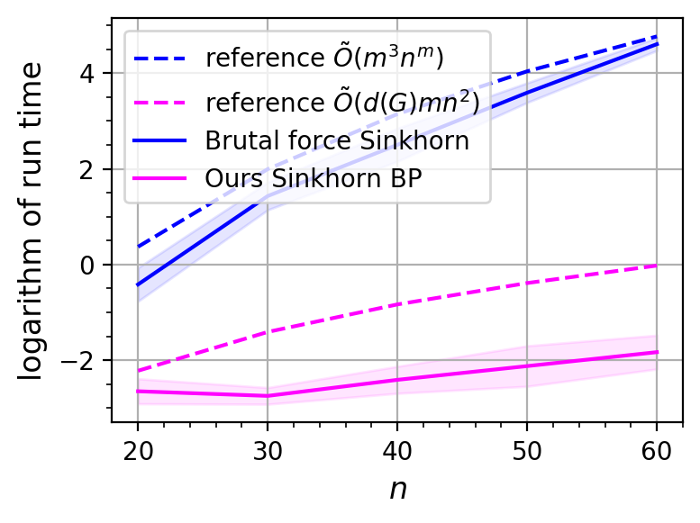
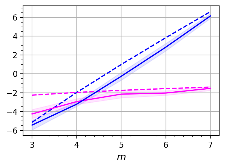
(a) Barycenter.

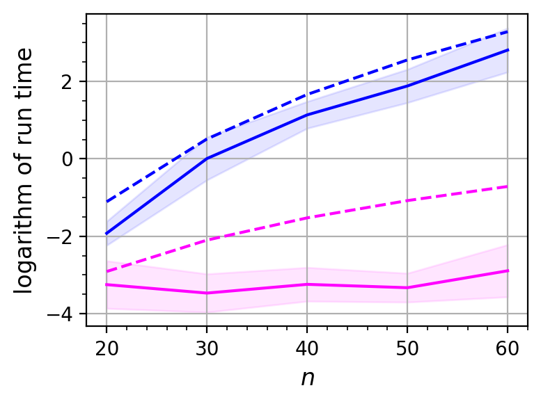
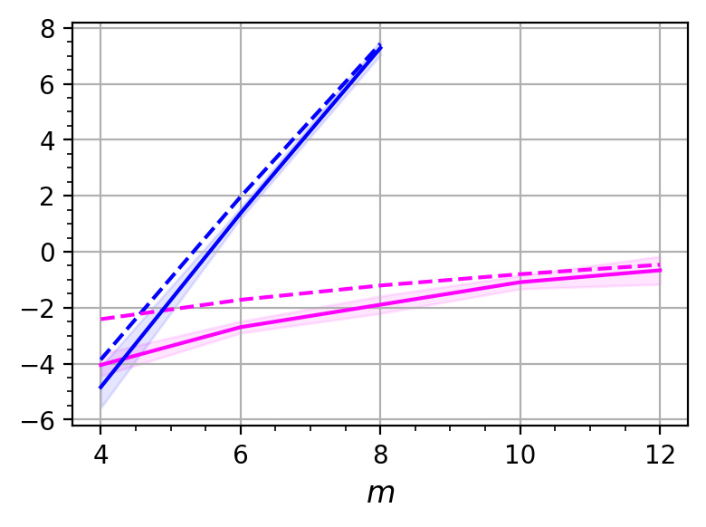
(b) Hidden Markov Model.

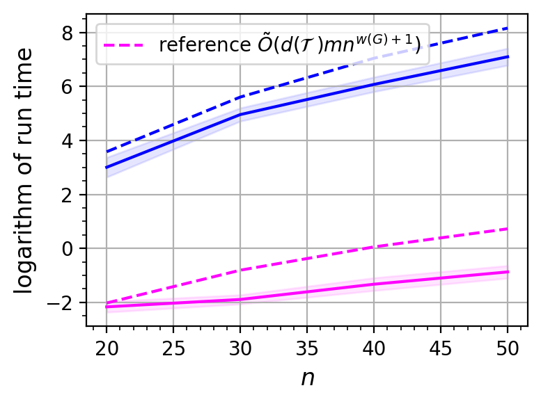
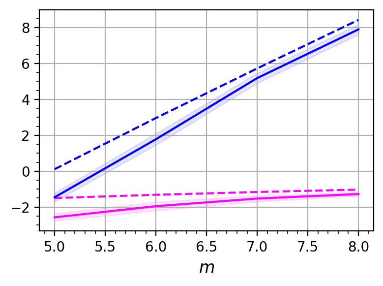
(c) Wasserstein least square.

Figure 5: Logarithm of total run time in seconds for brutal force Sinkhorn and Sinkhorn belief propagation. We use a smaller accuracy $\epsilon=0.2$ here.

References

• Altschuler et al. (2017) Altschuler, J., Niles-Weed, J., and Rigollet, P. Near-linear time approximation algorithms for optimal transport via Sinkhorn iteration. In Advances in neural information processing systems, pp. 1964–1974, 2017.
• Altschuler & Boix-Adsera (2020) Altschuler, J. M. and Boix-Adsera, E. Polynomial-time algorithms for multimarginal optimal transport problems with structure. arXiv preprint arXiv:2008.03006, 2020.