Discovery of interpretable structural model errors
by combining Bayesian sparse regression and data assimilation:
A chaotic Kuramoto-Sivashinsky test case

Abstract

Models of many engineering and natural systems are imperfect. The discrepancy between the mathematical representations of a true physical system and its imperfect model is called the model error. These model errors can lead to substantial differences between the numerical solutions of the model and the state of the system, particularly in those involving nonlinear, multi–scale phenomena. Thus, there is increasing interest in reducing model errors, particularly by leveraging the rapidly growing observational data to understand their physics and sources. Here, we introduce a framework named MEDIDA: Model Error Discovery with Interpretability and Data Assimilation. MEDIDA only requires a working numerical solver of the model and a small number of noise–free or noisy sporadic observations of the system. In MEDIDA, first the model error is estimated from differences between the observed states and model–predicted states (the latter are obtained from a number of one–time–step numerical integrations from the previous observed states). If observations are noisy, a data assimilation (DA) technique such as ensemble Kalman filter (EnKF)is employed to provide the analysis state of the system, which is then used to estimate the model error. Finally, an equation-discovery technique, here the relevance vector machine (RVM), a sparsity–promoting Bayesian method, is used to identify an interpretable, parsimonious, and closed–form representation of the model error. Using the chaotic Kuramoto–Sivashinsky (KS) system as the test case, we demonstrate the excellent performance of MEDIDA in discovering different types of structural/parametric model errors, representing different types of missing physics, using noise–free and noisy observations.

The discovery of the governing equations of physical systems is often based on the first principles, which has been the origin of most advances in science and engineering. However, in many important applications, some of the underlying physical processes are not well understood, and therefore, are missing or poorly represented in the mathematical models of such systems. Accordingly, these imperfect models (“models” hereafter) can merely closely track the dynamics of the true physical system (“system” hereafter), while failing to exactly represent it. Global climate models (GCMs) and numerical weather prediction (NWP) models are prominent examples of such models, often suffering from parametric and structural errors. The framework proposed here integrates machine learning (ML) and data assimilation (DA) techniques to discover close–form, interpretable representations of these model errors. This framework can leverage the ever-growing abundance of observational data to reduce the errors in models of nonlinear dynamical systems, such as the climate system.

I Introduction

The difference between the solution of the model and the system becomes prominent in many problems involving complex, nonlinear, multi-scale phenomena such as those in engineering (de Silva et al., 2020; Regazzoni et al., 2021; Willcox et al., 2021), thermo-fluids (Subramanian and Mahadevan, 2020; Duraisamy, 2021), and climate/weather prediction (Balaji, 2021; Schneider et al., 2021); see Levine and Stuart (2021) for an insightful overview. The deviation of the model from the system is called, in different communities, model uncertainty (structural and/or parametric), model discrepancy, model inadequacy, missing dynamics, or “model error”; hereafter, the latter is used.

Recently, many studies have focused on leveraging the rapid advances in ML techniques and availability of data (e.g., high-quality observations) to develop more accurate models. Several main approaches include learning fully data-driven (equation-free) models (e.g., Pathak et al., 2018; Vlachas et al., 2018; Dueben and Bauer, 2018; Weyn et al., 2019; Chattopadhyay et al., 2020; Arcomano et al., 2020; Chattopadhyay et al., 2020) or data-driven subgrid-scale closures (e.g., Ma et al., 2018; Rasp et al., 2018; Maulik et al., 2019; Brenowitz and Bretherton, 2019; Bolton and Zanna, 2019; Beck et al., 2019; Subel et al., 2021; Harlim et al., 2021; Guan et al., 2021). In a third approach, corrections to the state or its temporal derivative (tendency) are learned from deviation of the model predictions from the observations (Watson, 2019; Pawar et al., 2020; Pathak et al., 2020; Watt-Meyer et al., 2021; Bretherton et al., 2021). More specifically, the model is initialized with the observed state, integrated forward in time, and the difference between the predicted state and the observation at the later time is computed. Repeated many times, a correction scheme, e.g., a deep neural network (DNN), can be trained to nudge the model’s predicted trajectory (or tendency) to that of the system. To deal with observations with noise, a number of studies have integrated DA with DNNs (Bocquet et al., 2019; Farchi et al., 2021; Brajard et al., 2020; Chen and Li, 2021; Wikner et al., 2021; Chattopadhyay et al., 2021; Gottwald and Reich, 2021).

These studies often used DNNs, showing promising results for a variety of test cases. However, while powerfully expressive, DNNs are currently hard to interpret and often fail to generalize (especially extrapolate) when the systems’ parameters change (e.g., Rasp et al., 2018; Chattopadhyay et al., 2020; Guan et al., 2021; Mojgani and Balajewicz, 2021). The interpretability of models is crucial for robust, reliable, and generalizable decision–critical predictions or designs  (Willcox et al., 2021; Schneider et al., 2021). Posing the task of system identification as a linear regression problem, based on a library of nonlinear terms, exchanges the expressivity of DNNs for the sake of interpretability (Brunton et al., 2016; Rudy et al., 2017). The closed–form representation of the identified models and their parsimony (i.e., sparsity in the space of the employed library) is the key advantage of these methods, leading to highly interpretable models. A number of studies have used such methods to discover closed–form full models or closures (Rudy et al., 2017; Zhang and Lin, 2018; Schaeffer et al., 2018; Reinbold et al., 2020; Zanna and Bolton, 2020; Messenger and Bortz, 2021; Cortiella et al., 2021). While the results are promising, noisy data, especially in the chaotic regimes, significantly degrades the quality of the discovered models (Rudy et al., 2017; Reinbold et al., 2020; Messenger and Bortz, 2021; Cortiella et al., 2021).

So far, there has not been any work on discovering closed–form representation of model error using the differences between model predictions and observations (approach 3) or on combining the sparsity-promoting regression methods with DA to alleviate observation noise. Here, we introduce MEDIDA (Model Error Discovery with Interpretability and Data Assimilation), a general-purpose, data-efficient, non-intrusive framework to discover the structural (and parametric) model errors in the form of missing/incorrect terms of partial differential equations (PDEs). MEDIDA uses differences between predictions from a working numerical solver of the model and noisy sporadic (sparse in time) observations. The framework is built on two main ideas:

1. Discovering interpretable and closed–form model errors using relevance vector machine (RVM), a sparsity-promoting Bayesian regression method (Tipping, 2001),

2. Reducing the effects of observation noise using DA methods such as ensemble Kalman filter (EnKF) to generate the “analysis state”.

Below, we present the problem statement and introduce MEDIDA. Subsequently, its performance is demonstrated using a chaotic Kuramoto–Sivashinsky (KS)test case.

II Problem statement

Suppose the exact mathematical representation of a system is a nonlinear PDE,

$$\partial_{t}u(t)=g\left(u(t)\right),$$ (1)

in a continuous domain. Here, $u(t)$ is the state variable at time $t$. While (1) is unknown, we assume to have access to sporadic pairs of observations of the state variable $u^{o}$. These observations might be contaminated by measurement noise. The set of observed states at $t_{i}$ is denoted as $\left\{u^{o}\left({\color[rgb]{0,0,0}t_{i}-\Delta t_{i}}\right),u^{o}\left(t_{i}\right)\right\}_{i=1}^{n}$. Note that $t_{i}$ do not have to be equally spaced. Furthermore, $\Delta t_{i}$ should be similar for all $i$ but do not have to be the same (hereafter, we use $\forall i,\Delta t_{i}=\Delta t$ for convenience).

Moreover, suppose that we have a model of the system,

$$\partial_{t}u(t)=f\left(u(t)\right).$$ (2)

Without loss of generality (Levine and Stuart, 2021), we assume that the deviation of (2) from (1) is additive; we further assume that the deviation is only a function of the state (Bocquet et al., 2019; Farchi et al., 2021). Therefore, the model error is

$$h\left(u(t)\right):=g\left(u(t)\right)-f\left(u(t)\right).$$ (3)

Our goal is to find a closed–form representation of $h$ given a working numerical solver of (2) and noisy or noise–free observations $\left\{u^{o}\left(t_{i}-\Delta t\right),u^{o}\left(t_{i}\right)\right\}_{i=1}^{n}$.

III Framework: MEDIDA

MEDIDA has three main steps (Fig. 1): Step 1) Collecting sporadic observations of the system and numerically integrating the model forward for short-time (§III.1); Step 2) Construction and solving a regression problem using RVM (Tipping, 2001), which leads to the sparse identification of the model error (§III.2); Step 3) If observations are noisy, following step 1, stochastic EnKF (Asch et al., 2016; Law et al., 2015) is used to estimate an analysis state, an estimate of the system’s state, for Step 2 (§III.3). We emphasize that at no point MEDIDA needs any knowledge of the system (1). Also, note that other equation-discovery techniques and ensemble-based DA methods can be used in steps 2-3.

III.1 Interpretable model error

Consider the discretized (2):

$$\bm{u}^{m}(t_{i})=\bm{f}\left(\bm{u}^{o}(t_{i}-\Delta t)\right).$$ (4)

For brevity, we use the notation of an explicit scheme, but the scheme can also be implicit, as shown in the test case. The domain is discretized on the grid of $\bm{x}\in\mathbb{R}^{M}$. The observation at $t_{i}-\Delta t$, i.e., $\bm{u}^{o}(t_{i}-\Delta t)$, is the initial condition and $\bm{u}^{m}(t_{i})$ is the predicted state at time $t_{i}$ (Fig. 1a).

At each time $t_{i}$, subtracting the state predicted by the model ($\bm{u}^{m}(t_{i})$) from the observed state ($\bm{u}^{o}(t_{i})$) results in an approximation of the model error at $t_{i}$ (Fig. 1b):

$$\begin{aligned} \bm{h}\left(t_{i}\right)\approx\Delta\bm{u}_{i}:=(\bm{u}^{o}\left(t_{i}\right)-\bm{u}^{m}\left(t_{i}\right))/\Delta t.\end{aligned}$$ (5)

The difference between the states of the system and the model is similar to the analysis increment in the DA literature, where the best estimate of the state replaces $\bm{u}^{o}\left(t_{i}\right)$ in (5); see §III.3. The idea of accounting for model error through the analysis increment was first introduced by Leith (1978), and is at the core of many recent applications of ML aiming to nudge the model to its correct trajectory (Farchi et al., 2021), or to account for the model error (Carrassi and Vannitsem, 2011; Mitchell and Carrassi, 2015). However, in this manuscript, we aim to discover an interpretable representation of model error, $h\left(u\left(t\right)\right)$.

Note that to accurately discover $h\left(u(t)\right)$ as defined in (3), $\Delta\bm{u}_{i}$ should be dominated by the model error, and the contributions from numerical errors (in obtaining $\bm{u}^{m}\left(t_{i}\right)$) and measurement errors (in $\bm{u}^{o}(t_{i})$) should be minimized as much as possible. As discussed in §III.3, DA can be utilized to reduce the contributions from the observation noise. Computing $\Delta\bm{u}_{i}$ after only one $\Delta t$ prevents accumulation of numerical error from integrating (4). Moreover, this avoids nonlinear growth of the model error, and its further entanglement with truncation errors, which can complicate the discovery of just model error. Therefore, in MEDIDA, the model time step and observation intervals are set to be the same. Note that while the size of $\Delta t$ could be restricted by availability of the observation pairs, increasing $M$ can be used to reduce truncation errors from spatial discretizations.

Integrating (4) from $\bm{u}^{o}(t_{i}-\Delta t)$ and computing $\Delta\bm{u}_{i}$ from (5) are repeated for $n$ samples (step 1), and the vectors of model error are stacked to form $\Delta\bm{u}\in\mathbb{R}^{nM}$ (step 2); see Fig. 1a-b. Similar to past studies (Rudy et al., 2017; Zhang and Lin, 2018, 2021; Reinbold et al., 2020), we further assume that the model error spans over the space of the bases or training vectors, i.e.,

$$h\left(u(t)\right)={c}_{1}{\phi}_{1}+\cdots+{c}_{q}{\phi}_{q},$$ (6)

where ${\phi}_{i}$ is a linear or nonlinear function of the state variable, the building block of the library of training bases $\left\{{\phi}_{k}\left({u(t)}\right)\right\}_{k=1}^{q}$. Selection of the bases should be guided by the physical understanding of the system and the model.

Here, in the discretized form, we assume that $\bm{\Phi}\left(\bm{u}\right)$ is a linear combination of polynomial terms up to $p^{\textit{th}}$-order and spatial derivatives up to $d^{\textit{th}}$-order, i.e.,

$$\bm{\Phi}_{k}\left(\bm{u}\right)=\bm{u}^{{r}}\odot\bm{D}^{s}_{x}\bm{u};{{r}\in\left\{0,\cdots,p\right\},{s}\in\left\{0,\cdots,d\right\}},$$ (7)

where in $\bm{u}^{{r}}$ each element of $\bm{u}$ is raised to the power of ${r}$, $\bm{D}^{s}_{x}\bm{u}$ denotes the ${s}^{\textit{th}}$ spatial derivative of $\bm{u}$, and $\odot$ is the element-wise (Hadamard) product. Therefore, the model error lies on the space of library of the training bases evaluated using the observed state at each $t_{i}$, $\bm{\Phi}\left(\bm{u}^{o},t_{i}\right)\in\mathbb{R}^{M\times q}$. For all the $n$ samples, the library of the bases are stacked to form $\bm{\Phi}\left(\bm{u}^{o}\right)\in\mathbb{R}^{nM\times q}$ (Fig. 1b).

At the end of step 2, the regression problem for discovery of model error is formulated as

$$\bm{{c}}^{*}={} \underset{\bm{{c}}}{arg\text{min}}\left\|\Delta\bm{u}-\bm{\Phi}\left(\bm{u}^{o}\right)\bm{{c}}\right\|_{2},$$ (8)

where $\bm{{c}}\in\mathbb{R}^{q}$ is the vector of coefficients corresponding to the training bases, and $\bm{{c}}^{*}={\left[c^{*}_{1},c^{*}_{2},\cdots,c^{*}_{q}\right]}^{\top}$ is a minimizer of the regression problem, i.e., the vector of coefficients of the model error. Finally, the discovered (corrected) model is identified as

$$\partial_{t}u(t)=f\left(u(t)\right)+\Sigma_{k=1}^{q}c^{*}_{k}{\phi}_{k}\left(u(t)\right).$$ (9)

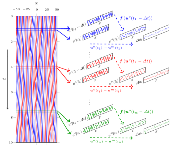
(a) Step 1: Observation and model prediction

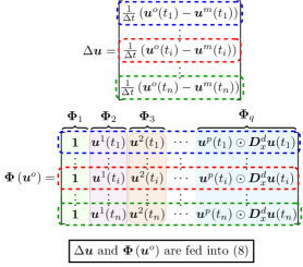
(b) Step 2: Forming the regression problem

(c) Step 3: EnKF is used to assimilate noisy observations for step 2

Figure 1: The schematic of MEDIDA, presented in the context of the test case in §IV. LABEL:sub@fig:discovery Step 1: $n$ pairs of state variables are sampled uniformly or non-uniformly at $t_{i}$ from observations (of the system (1)) to obtain $\left\{\bm{u}^{o}\left(t_{i}-\Delta t\right),\bm{u}^{o}\left(t_{i}\right)\right\}_{i=1}^{n}$. The model (4) is integrated numerically for one time-step from each $\bm{u}^{o}\left(t_{i}-\Delta t\right)$ to predict $\bm{u}^{m}\left(t_{i}\right)$. For each sample, at $t_{i}$, the difference between the predicted and observed state is used to compute $\Delta\bm{u}_{i}$ (5), an approximation of model error. LABEL:sub@fig:discovery2 Step 2: $\left\{\Delta\bm{u}_{i}\right\}_{i=1}^{n}$ are stacked to form $\Delta\bm{u}$. Moreover, the library of bases $\bm{\Phi}\left(\bm{u}^{o}\right)$, consisting of selected $q$ linear and nonlinear bases evaluated at $\left\{\bm{u}^{o}\left(t_{i}\right)\right\}_{i=1}^{n}$, is formed. Here, the library in (7) is used, but the bases with any arbitrary functional form could be used depending on the anticipated form of the model error. $\Delta\bm{u}$ and $\bm{\Phi}$ are then fed into the RVM (or other equation-discovery methods) to compute $\bm{c}^{*}$ for minimizing the loss function (8). The corrected model is then identified using $\bm{c}^{*}$ as Eq. (9). LABEL:sub@fig:assimilation Step 3: If observations are noisy, DA is used to provide an “analysis state” $\left\{\bm{u}^{a}\left(t_{i}\right)\right\}_{i=1}^{n}$ to be used in place of $\left\{\bm{u}^{o}\left(t_{i}\right)\right\}_{i=1}^{n}$ for computing $\Delta\bm{u}$ and $\bm{\Phi}$ in Steps 1-2. Here we use a stochastic EnKF for DA: For each sample $i$, the noisy observation is perturbed by Gaussian white noise with inflated standard deviation $\sigma_{b}$ to generate an ensemble of size $N$. Each ensemble member $k$ is numerically evolved by the model, $\left\{\bm{f}\left(\bm{u}^{o}_{k}(t_{i}-\Delta t)\right)\right\}_{k=1}^{N}$, to generate the ensemble of model prediction $\left\{\bm{u}_{k}^{m}\left(t_{i}\right)\right\}_{k=1}^{N}$. Observations at time $t_{i}$ are also perturbed by Gaussian white noise with standard deviation $\sigma_{obs}$ to generate the ensemble $\left\{\bm{u}_{k}^{o}\left(t_{i}\right)\right\}_{k=1}^{N}$. These two ensembles are then used to compute the background covariance matrix $\bm{P}$, Kalman gain $\bm{K}$, and finally, the analysis state $\overline{\bm{u}^{a}}(t_{i})$; overbars indicate ensemble mean and $\mathop{\mathbb{E}}\left[.\right]$ denotes expectation. $\Delta\bm{u}$ and $\bm{\Phi}$ in steps 1-2 are then computed using $\overline{\bm{u}^{a}}(t_{i})$.

III.2 Solution of the regression problem

In this study, we use RVM (Tipping, 2001) to compute $\bm{{c}}^{*}$ in (8) for inputs of $\Delta\bm{u}$ and $\bm{\Phi}\left(\bm{u}^{o}\right)$. RVM leads to a sparse identification of columns of $\bm{\Phi}$ with posterior distribution of the corresponding weights, i.e., the relevant vectors. See Zhang and Lin (2018) for a detailed discussion in the context of PDEs discovery.

The breakthrough in equation-discovery originates in introduction of parsimony (Brunton et al., 2016). While the original LASSO-type regularization has yielded promising results in a broad range of applications, RVMs have been found to achieve the desired sparsity by a more straightforward hyper-parameter tuning and a relatively lower sensitivity to noise (Zhang and Lin, 2018; Zanna and Bolton, 2020; Rudy and Sapsis, 2021). The hyper-parameter in RVMs is a threshold to prune the bases with higher posterior variance, i.e., highly uncertain bases are removed. To avoid over-fitting, we choose the hyper-parameter as a compromise between the sparsity and accuracy of the corrected model at the elbow of the L-curve, following Mangan et al. (2017).

III.3 Data assimilation

Steps 1-2 described above suffice to find an accurate corrected model (9) if the fully observed state is noise–free. However, noise can cause substantial challenges in the sparse identification of nonlinear systems, a topic of ongoing research (Rudy et al., 2017; Goyal and Benner, 2021; Rudy and Sapsis, 2021; Reinbold et al., 2020; Schaeffer et al., 2018). In MEDIDA, we propose to use DA, a powerful set of tools to deal with noisy and partial observation (spatio-–temporal sparsity). Here, we use stochastic EnKF (Evensen, 1994) (Fig. 1c). In this study, we assume that that observations of the full state are available; i.e., $\mathcal{H}(u\left(t\right))=u\left(t\right)\in\mathbb{R}^{M}$ where $\mathcal{H}(.)$ is the observation operator. Dealing with partial observations and more general forms of observation errors (e.g., as in Hamilton et al. Hamilton et al. (2019)) remains subject of future investigations.

The result of this step is the analysis state used to construct the vector of model error and the library of the bases (Fig. 1b).

At each sample time $t_{i}-\Delta t$, the observations are further perturbed with Gaussian white noise to obtain an ensemble of size $N$ of the initial conditions,

$$\bm{u}^{o}_{k}(t_{i}-\Delta t)=\bm{u}^{o}(t_{i}-\Delta t)+\mathcal{N}\left(0,\sigma_{b}^{2}\right),$$ (10)

where $\sigma_{b}$ is standard deviation of the observation noise ($\sigma_{obs}$) times an inflation factor (Anderson and Anderson, 1999; Asch et al., 2016), and $k$ denotes the $k^{\textit{th}}$ ensemble member.

Subsequently, the model is evolved for each of these ensemble members, i.e., ${\bm{u}_{k}^{m}}(t_{i})=\bm{f}\left(\bm{u}^{o}_{k}(t_{i}-\Delta t)\right)$. This ensemble of model prediction is used to construct the background covariance matrix as

$$\begin{aligned} \bm{P}&=\mathop{\mathbb{E}}\left[\left(\bm{u}_{k}^{m}(t_{i})-\overline{\bm{u}^{m}}(t_{i})\right){\left(\bm{u}_{k}^{m}(t_{i})-\overline{\bm{u}^{m}}(t_{i})\right)}^{\top}\right],\\ \end{aligned}$$ (11)

where $\overline{\bm{u}^{m}}(t_{i})$ is the ensemble average of the model prediction, and $\mathop{\mathbb{E}}\left[.\right]$ denotes the expected value. Having the observation operator to be linear, and non-sparse, the Kalman gain, $\bm{K}\in\mathbb{R}^{M\times M}$, is then calculated as,

$$\begin{aligned} \bm{K}&=\bm{P}\left(\bm{P}+\sigma_{obs}\bm{I}\right)^{-1},\\ \end{aligned}$$ (12)

where $\bm{I}\in\mathbb{R}^{M\times M}$ is the identity matrix.

For each sample at the prediction time $t_{i}$, the $k^{\textit{th}}$ member of the ensemble of the observations is generated as

$$\bm{u}^{o}_{k}(t_{i})=\bm{u}^{o}(t_{i})+\mathcal{N}\left(0,\sigma_{obs}^{2}\right).$$ (13)

Note that while the EnKF can be used for non–Gaussian observation noise, the method would be sub–optimal and may require further modification (Carrassi et al., 2018). Hereon, we limit our experiments to Gaussian noise.

Finally, the $k^{\textit{th}}$ member of the ensemble of the analysis state is

$$\begin{aligned} \bm{u}^{a}_{k}(t_{i})=\bm{u}^{m}_{k}(t_{i})+\bm{K}\left(\bm{u}^{o}_{k}(t_{i})-\bm{u}^{m}_{k}(t_{i})\right).\end{aligned}$$ (14)

The process of EnKF assimilates the noisy observations to the background forecast obtained from the model, $\bm{u}^{m}_{k}(t_{i})$. Subsequently, the ensemble average of the analysis states, $\overline{\bm{u}^{a}}(t_{i})$, is treated as a close estimate of the true state of the system, $\bm{u}^{o}\left(t_{i}\right)$ in §III.1.

Similarly, the difference between the ensemble averages of the analysis state and the model prediction, i.e.,

$$\Delta\bm{u}(t_{i})=(\overline{\bm{u}^{a}}(t_{i})-\overline{\bm{u}^{m}}(t_{i}))/\Delta t,$$ (15)

replaces (5) and is fed into the algorithm of §III.1.

There are a few points about this DA step that need to be further clarified. First, as discussed in §III.1, the model is evolved for only one time step. Although this may hinder the traditional spin–up period used in EnKF, as a compromise, we resort to a large ensemble and inflation to ensure successful estimation of the state.

Second, for MEDIDA to work well, (15) should be dominated by model error. However, the inevitable presence of other sources of error, notably the observation errors, generally leads to an overestimation of the actual model error; see Carrassi and Vannitsem (2011) for discussions and remedies.

Finally, note that ensemble Kalman smoother (EnKS) (Evensen and van Leeuwen, 2000) is shown to be more suitable for offline pre-processing of the data used in ML models (Chen and Li, 2021); however; in MEDIDA, the model is evolved for a single time step, therefore, we expect that EnKS and EnKF to behave similarly.

III.4 Performance metric

To quantify the accuracy of MEDIDA, we use the normalized distance between the vector of coefficients, defined as

$$\varepsilon_{m}=\frac{\left\|{\bm{{c}}}_{s}-\bm{{c}}_{m}\right\|_{2}}{\left\|{\bm{{c}}}_{s}\right\|_{2}}\;\;\mathrm{and}\;\;\varepsilon^{*}=\frac{\left\|{\bm{{c}}}_{s}-\bm{{c}}^{*}\right\|_{2}}{\left\|{\bm{{c}}}_{s}\right\|_{2}},$$ (16)

where ${\bm{{c}}}_{s}$, $\bm{{c}}_{m}$, $\bm{{c}}^{*}$ are coefficient vectors of the system (1), the model (2), and the corrected model (9)(Rudy et al., 2017; Reinbold et al., 2020). The $i^{\textit{th}}$ element of the coefficient vector is a scalar corresponding to the $i^{\textit{th}}$ term in the equation. Quantitatively, the goal is to achieve $\varepsilon^{*}\ll\varepsilon_{m}$. Note that the implicit assumption in this metric is that the model and the model error can be expressed on the space spanned by the bases of the library.

IV Test case: KS equation

To evaluate the performance of MEDIDA, we use a chaotic KS system, a challenging test case for system identification, particularly from noisy observations (Rudy et al., 2017; Reinbold et al., 2020). The PDE is

$$\partial_{t}u+u\partial_{x}u+\partial^{2}_{x}u+\partial^{4}_{x}u=0,$$ (17)

where $u\partial_{x}u$ is convection, $\partial_{x}^{2}{u}$ is anti-diffusion (destabilizing), and $\partial_{x}^{4}{u}$ is hyper-diffussion (stabilizing). The domain is periodic, $u\left(0,t\right)=u\left(L,t\right)$. We use $L=32\pi$, which leads to a highly chaotic system (Pathak et al., 2018; Khodkar and Hassanzadeh, 2021).

Here, (17) is the system. We have created 9 (imperfect) models as shown in Table 1. In cases 1-3, one of the convection, anti-diffusion, or hyper-diffusion term is entirely missing (i.e., structural uncertainty). In cases 4-6, some or all of the coefficients of the system are incorrect (parametric uncertainty). Finally, in cases 7-9, a mixture of parametric and structural uncertainties, with missing and extra terms, is present.

The system and the models are numerically solved using different time-integration schemes and time-step sizes to introduce additional challenges and a more realistic test case. To generate $\bm{u}^{o}$, (17) is integrated with the exponential time-differencing fourth-order Runge-Kutta (Kassam and Trefethen, 2005) with time-step $\Delta t^{o}$ (in Fig. 1a, $1t=10^{3}\Delta t^{o}$). The models are integrated with second-order Crank-Nicolson and Adams-Bashforth schemes with $\Delta t^{m}=\Delta t=5\Delta t^{o}$. For both system and models, $M=1024$ Fourier modes are used (different discretizations or $M$ for system and models could have been used too). $\bm{u}^{o}$ is collected after a spin-up period of $\tau=200\Delta t$ and uniformly at $t_{i}=i\tau$. $\bm{\Phi}$, is constructed with $d=4$ and $p=4$ as defined in (7). Open-source codes are used to generate $\bm{\Phi}$ (Rudy et al., 2017) and solve (8) using RVM (Zanna and Bolton, 2020).

IV.1 Noise–free observations

First, we examine the performance of MEDIDA for noise–free observations (only steps 1-2). The motivation is two–fold: i) to test steps 1-2 before adding the complexity of noisy observations/DA, and ii) in many applications, an estimate of $\bm{u}^{o}$ is already available (see §V).

Here, $\bm{u}^{o}$ are from the numerical solutions of (17). The models, MEDIDA-corrected models, and the corresponding errors for $n=100$ samples show $\varepsilon^{*}<2\%$, between 40 to 200 times improvement compared to $\varepsilon_{m}$ (Table 1).

To conclude, MEDIDA is a data-efficient framework. Its performance is insensitive to $n$, such that $\varepsilon^{*}$ changes by $0.1\%$ for $n\in\left\{10,100,1000\right\}$. There are two reasons for this: i) RVM is known to be data-efficient (compared to DNNs) (Bishop, 2006), and ii) each grid point at $t_{i}$ provides a data-point, i.e., a row in $\Delta\bm{u}$ and $\bm{\Phi}$, although these are not all independent/uncorrelated data-points.

Table 1: MEDIDA-corrected models from noise–free and noisy observations of the KS system: $0=\partial_{t}u+u\partial_{x}u+\partial^{2}_{x}u+\partial^{4}_{x}u$. $\varepsilon_{m}$ and $\varepsilon^{*}$ are defined in (16). For the noisy cases, $\sigma_{b}=20\sigma_{obs}$, and the ensemble size is $N=10M$, except for cases 3, 6, and 9 with $N=200M$, $100M$, and $500M$, respectively.

#	Model:                            $0=\partial_{t}u+$	$\varepsilon_{m}\left[\%\right]$	Corrected model (noise–free):        $0=\partial_{t}u+$	$\varepsilon^{*}\left[\%\right]$	Corrected model (noisy):           $0=\partial_{t}u+$	$\varepsilon^{*}\left[\%\right]$
1	$\partial^{2}_{x}u+\partial^{4}_{x}u$	$57.74$	$\numprint{0.9740}u\partial_{x}u+\partial^{2}_{x}u+\partial^{4}_{x}u$	$1.50$	$0.98u\partial_{x}u+\partial^{2}_{x}u+\partial^{4}_{x}u$	$1.43$
2	$u\partial_{x}u+\partial^{4}_{x}u$	$57.74$	$u\partial_{x}u+\numprint{0.9933}\partial^{2}_{x}u+\partial^{4}_{x}u$	$0.39$	$u\partial_{x}u+0.98\partial^{2}_{x}u+\partial^{4}_{x}u$	$0.98$
3	$u\partial_{x}u+\partial^{2}_{x}u$	$57.74$	$u\partial_{x}u+\partial^{2}_{x}u+\numprint{1.0187}\partial^{4}_{x}u$	$1.08$	$u\partial_{x}u+\partial^{2}_{x}u+1.02\partial^{4}_{x}u$	$0.98$
4	$0.5u\partial_{x}u+\partial^{2}_{x}u+\partial^{4}_{x}u$	$28.87$	$\numprint{0.9870}u\partial_{x}u+\partial^{2}_{x}u+\partial^{4}_{x}u$	$0.75$	$0.99u\partial_{x}u+\partial^{2}_{x}u+\partial^{4}_{x}u$	$0.63$
5	$u\partial_{x}u+0.5\partial^{2}_{x}u+\partial^{4}_{x}u$	$28.87$	$u\partial_{x}u+\numprint{0.9976}\partial^{2}_{x}u+\partial^{4}_{x}u$	$0.14$	$u\partial_{x}u+0.98\partial^{2}_{x}u+\partial^{4}_{x}u$	$0.99$
6	$u\partial_{x}u+\partial^{2}_{x}u+0.5\partial^{4}_{x}u$	$28.87$	$u\partial_{x}u+\partial^{2}_{x}u+\numprint{1.0025}\partial^{4}_{x}u$	$0.14$	$u\partial_{x}u+\partial^{2}_{x}u+1.00\partial^{4}_{x}u$	$0.15$
7	$0.5u\partial_{x}u+2\partial^{4}_{x}u$	$86.60$	$\numprint{0.9732}u\partial_{x}u+\numprint{0.9995}\partial^{2}_{x}u+\partial^{4}_{x}u$	$1.55$	$0.98u\partial_{x}u+0.98\partial^{2}_{x}u+\partial^{4}_{x}u$	$1.63$
8	$u\partial_{x}u+\partial^{2}_{x}u+0.5\partial^{3}_{x}u+\partial^{4}_{x}u$	$28.87$	$u\partial_{x}u+\partial^{2}_{x}u+\partial^{4}_{x}u$	$0.28$	$u\partial_{x}u+\partial^{2}_{x}u-\numprint{0.0144}\partial^{3}_{x}u+\partial^{4}_{x}u$	$0.83$
9	$u\partial_{x}u+\partial^{2}_{x}u+0.5\partial^{3}_{x}u$	$64.55$	$u\partial_{x}u+\partial^{2}_{x}u-\numprint{0.0131}\partial^{3}_{x}u+\numprint{1.0168}\partial^{4}_{x}u$	$1.29$	$u\partial_{x}u+\partial^{2}_{x}u-\numprint{0.0095}\partial^{3}_{x}u+\numprint{1.0014}\partial^{4}_{x}u$	$0.55$

IV.2 Noisy observations

Next, we examine the performance of MEDIDA for noisy observations, obtained from adding noise to the numerical solution of KS: $u^{o}(t)=u(t)+\mathcal{N}\left(0,\sigma_{obs}^{2}\right).$ Here, $\sigma_{obs}/\sigma_{u}=0.01$, where $\sigma_{u}$ is the standard deviation of the state (equivalent to $0.1$ following the methodology in (Reinbold et al., 2020; Kaheman et al., 2020)). Without step 3 (DA), the model error discovery fails, leading to many spurious terms and $\varepsilon^{*}$ of $O(10\%)-O(100\%)$, comparable or even worse than the model error, $\varepsilon_{m}$ (Fig. 2).

Table 1 shows the corrected models (with step 1-3). With $N=10M$, in all cases except for 3, 6, and 9, $\varepsilon^{*}<2\%$, between 30 to 60 times lower than $\varepsilon_{m}$. For those 3 cases, increasing $N$ further reduces $\varepsilon^{*}$ (Fig. 2), leading to the discovery of accurate models with $\varepsilon^{*}<1\%$ at large ensembles with $N=100M-500M$ (Table 1). Note that one common aspect of these cases is that the model is missing or mis-representing the hyper-diffusion term. The larger $N$ is needed to further reduce the noise in the analysis state to prevent amplification of the noise due to the higher-order derivative of this term. It should also be highlighted that while $N$ at the order of $M$ or larger might seem impractical, each ensemble member requires only one time-step integration (thus, a total of $nN$ time steps).

MEDIDA is found to be data-efficient in these experiments too. Like before, $\varepsilon^{*}$ changes by $0.1\%$ for $n\in\left\{10,100,1000\right\}$ for all cases except for 3, 6, and 9. For these 3 cases, $\varepsilon^{*}$ improves by about $10\%$ as $n$ is increased from $10$ to $100$, but then changes by only $0.1\%$ when $n$ is further increased to $1000$.

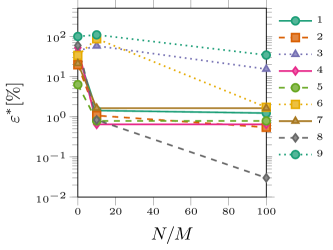
Figure 2: Improvement in the performance of MEDIDA as the ensemble size, $N$, is increased ($n=100$). $N/M=0$ corresponds to no DA. $\varepsilon^{*}$ for cases 3 and 9 further drops to $0.98\%$ and $0.55\%$ using larger ensembles of $N=200M$ and $N=500M$, respectively (Table 1).

V Discussion and Summary

We introduced MEDIDA, a data–efficient, and non–intrusive framework to discover interpretable, closed–form structural (or parametric) model error for chaotic systems. MEDIDA only needs a working numerical solver of the model and $n$ sporadic pairs of noise–free or noisy observations of the system. Model error is estimated from differences between the observed and predicted states (obtained from one–time–step integration of the model from earlier observations). A closed–form representation of the model error is estimated using an equation-discovery technique such as RVM. MEDIDA is expected to work accurately if i) the aforementioned differences are dominated by model error and not by numerical (discretization) error or observation noise, and ii) the library of the bases is adequate (further discussed below). Regarding (i), the numerical error can be reduced by using higher numerical resolutions while the observation noise can be tackled using DA techniques such as EnKF.

The performance of MEDIDA is demonstrated using a chaotic KS system for both noise–free and noisy observations. In the absence of noise, even with a small $n$, MEDIDA shows excellent performance and accurately discovers linear and nonlinear model errors, leading to corrected models that are very close to the system. These results already show the potential of MEDIDA as in some important applications, noise–free estimates of the system (reanalysis states) are routinely generated and are available; this is often the case for atmosphere and some other components of the Earth systemMuñoz Sabater et al. (2021); Hersbach et al. (2020); Fan et al. (2006). For example, such reanalysis states have been recently used to correct the model errors of an NWP model (Watt-Meyer et al., 2021), a quasi–geostrophic (QG) model (Farchi et al., 2021), and a modular arbitrary–order–ocean–atmosphere model (MAOOAM) (Brajard et al., 2021).

In the presence of noise, the model error could not be accurately discovered without DA. Once EnKF is employed, MEDIDA accurately discovers linear and nonlinear model errors. A few cases with model errors involving linear but $4^{\textit{th}}$-order derivatives require larger ensembles. This is because higher-quality analysis states are needed to avoid amplification of any remaining noise as a result of high-order derivatives.

Although the number of ensemble members used in MEDIDA is more than what it is commonly used in operational DA, the associated cost is tractable, since each ensemble is evolved only for one time step. This is another advantage of evolving the model for only one time step, which as discussed before, and is also motivated by reducing the accumulation of truncation errors and nonlinear growth of the model errors. Still, if needed, inexpensive surrogates of the model that could provide accurate one–time–step forecasts can be used to efficiently produce the ensembles (Chattopadhyay et al., 2021; Pathak et al., 2022).

Also, note that in EnKF, ensemble members are evolved using the model. If the model error is large, the analysis state might be too far from the system’s state, degrading the performance of MEDIDA. In all cases examined here, even though the model errors are large, with large-enough ensembles, the approximated analysis states are accurate enough to enable MEDIDA to discover the missing or inaccurate terms. However, in more complex systems, this might become a challenge that requires devising new remedies. One potential resolution is an iterative procedure, in which the analysis state is generated and a corrected model is identified, which is then used to produce a new analysis state and a new corrected model, and this continues until convergence. Although such iterative approaches currently lack proof of convergence, they have shown promises in similar settings (Brunton et al., 2016; Schaeffer, 2017; Hamilton et al., 2019; Schneider et al., 2020); for example, Hamilton et al. (2019) update the error in the observations iteratively until the convergence of the estimated state from the EnKF. The corresponding cost and possible convergence properties of such an iterative approach for MEDIDAremain to be investigated. Similarly, other methods for dealing with noise in equation discovery (e.g., Reinbold et al., 2020, 2021; Goyal and Benner, 2021) could also be integrated into MEDIDA.

The choice of an adequate library for RVM is crucial in MEDIDA. Although an exhaustive library of the training vectors with any arbitrary bases is straightforward, it quickly becomes computationally intractable. Any a priori knowledge of the system, such as locality, homogeneity (Bocquet et al., 2019), Galilean invariance, and conservation properties (Zhang and Lin, 2018) can be considered to construct a concise library. Conversely, the library can be expanded to “explore the computational universe”, e.g., using gene expression programming (Vaddireddy et al., 2020). Even further, additional constraints, such as stability of the corrected model, can be imposed (Mojgani and Balajewicz, 2020; Loiseau and Brunton, 2018; Chen, 2020). Effective strategies for the selection of an adequate and concise library can be investigated in future work using more complex test cases.

Finally, beyond dealing with noisy observations, another challenge in the discovery of interpretable model errors is approximating the library given spatially sparse observations. Approaches that leverage auto-differentiation for building the library in equation discovery have recently shown promising results (Chen et al., 2021), and can be integrated into MEDIDA.

MEDIDA is shown to work well for a widely used but simple chaotic prototype, the KS system. The next step will be investigating the performance of MEDIDA for more complex test cases, such as a two-layer quasi-geostrophic model. Scaling MEDIDA to more complex, higher dimensional systems will enable us to discover interpretable model errors for GCMs, NWP models, and other models of the climate system.