Bicep / Keck XV: THE Bicep3 CMB POLARIMETER AND THE FIRST THREE YEAR DATA SET

P. A. R. Ade School of Physics and Astronomy, Cardiff University, Cardiff, CF24 3AA, United Kingdom Z. Ahmed Kavli Institute for Particle Astrophysics and Cosmology, SLAC National Accelerator Laboratory, 2575 Sand Hill Rd, Menlo Park, California 94025, USA M. Amiri Department of Physics and Astronomy, University of British Columbia, Vancouver, British Columbia, V6T 1Z1, Canada D. Barkats Center for Astrophysics, Harvard & Smithsonian, Cambridge, MA 02138, U.S.A R. Basu Thakur Department of Physics, California Institute of Technology, Pasadena, California 91125, USA C. A. Bischoff Department of Physics, University of Cincinnati, Cincinnati, Ohio 45221, USA D. Beck Kavli Institute for Particle Astrophysics and Cosmology, SLAC National Accelerator Laboratory, 2575 Sand Hill Rd, Menlo Park, California 94025, USA Department of Physics, Stanford University, Stanford, California 94305, USA J. J. Bock Department of Physics, California Institute of Technology, Pasadena, California 91125, USA Jet Propulsion Laboratory, Pasadena, California 91109, USA H. Boenish Center for Astrophysics, Harvard & Smithsonian, Cambridge, MA 02138, U.S.A E. Bullock Minnesota Institute for Astrophysics, University of Minnesota, Minneapolis, Minnesota 55455, USA V. Buza Kavli Institute for Cosmological Physics, University of Chicago, Chicago, IL 60637, USA J. R. Cheshire IV Minnesota Institute for Astrophysics, University of Minnesota, Minneapolis, Minnesota 55455, USA J. Connors Center for Astrophysics, Harvard & Smithsonian, Cambridge, MA 02138, U.S.A J. Cornelison Center for Astrophysics, Harvard & Smithsonian, Cambridge, MA 02138, U.S.A M. Crumrine School of Physics and Astronomy, University of Minnesota, Minneapolis, Minnesota 55455, USA A. Cukierman Department of Physics, Stanford University, Stanford, California 94305, USA Kavli Institute for Particle Astrophysics and Cosmology, SLAC National Accelerator Laboratory, 2575 Sand Hill Rd, Menlo Park, California 94025, USA E. V. Denison National Institute of Standards and Technology, Boulder, Colorado 80305, USA M. Dierickx Center for Astrophysics, Harvard & Smithsonian, Cambridge, MA 02138, U.S.A L. Duband Service des Basses Températures, Commissariat à l’Energie Atomique, 38054 Grenoble, France M. Eiben Center for Astrophysics, Harvard & Smithsonian, Cambridge, MA 02138, U.S.A S. Fatigoni Department of Physics and Astronomy, University of British Columbia, Vancouver, British Columbia, V6T 1Z1, Canada J. P. Filippini Department of Physics, University of Illinois at Urbana-Champaign, Urbana, Illinois 61801, USA Department of Astronomy, University of Illinois at Urbana-Champaign, Urbana, Illinois 61801, USA S. Fliescher School of Physics and Astronomy, University of Minnesota, Minneapolis, Minnesota 55455, USA N. Goeckner-Wald Department of Physics, Stanford University, Stanford, California 94305, USA D. C. Goldfinger Center for Astrophysics, Harvard & Smithsonian, Cambridge, MA 02138, U.S.A J. Grayson Department of Physics, Stanford University, Stanford, California 94305, USA P. Grimes Center for Astrophysics, Harvard & Smithsonian, Cambridge, MA 02138, U.S.A G. Hall School of Physics and Astronomy, University of Minnesota, Minneapolis, Minnesota 55455, USA G. Halal Department of Physics, Stanford University, Stanford, California 94305, USA M. Halpern Department of Physics and Astronomy, University of British Columbia, Vancouver, British Columbia, V6T 1Z1, Canada E. Hand Department of Physics, University of Cincinnati, Cincinnati, Ohio 45221, USA S. Harrison Center for Astrophysics, Harvard & Smithsonian, Cambridge, MA 02138, U.S.A S. Henderson Kavli Institute for Particle Astrophysics and Cosmology, SLAC National Accelerator Laboratory, 2575 Sand Hill Rd, Menlo Park, California 94025, USA S. R. Hildebrandt Department of Physics, California Institute of Technology, Pasadena, California 91125, USA Jet Propulsion Laboratory, Pasadena, California 91109, USA G. C. Hilton National Institute of Standards and Technology, Boulder, Colorado 80305, USA J. Hubmayr National Institute of Standards and Technology, Boulder, Colorado 80305, USA H. Hui Department of Physics, California Institute of Technology, Pasadena, California 91125, USA K. D. Irwin Department of Physics, Stanford University, Stanford, California 94305, USA Kavli Institute for Particle Astrophysics and Cosmology, SLAC National Accelerator Laboratory, 2575 Sand Hill Rd, Menlo Park, California 94025, USA National Institute of Standards and Technology, Boulder, Colorado 80305, USA J. Kang Department of Physics, Stanford University, Stanford, California 94305, USA Department of Physics, California Institute of Technology, Pasadena, California 91125, USA K. S. Karkare Center for Astrophysics, Harvard & Smithsonian, Cambridge, MA 02138, U.S.A Kavli Institute for Cosmological Physics, University of Chicago, Chicago, IL 60637, USA E. Karpel Department of Physics, Stanford University, Stanford, California 94305, USA S. Kefeli Department of Physics, California Institute of Technology, Pasadena, California 91125, USA S. A. Kernasovskiy Department of Physics, Stanford University, Stanford, California 94305, USA J. M. Kovac Center for Astrophysics, Harvard & Smithsonian, Cambridge, MA 02138, U.S.A Department of Physics, Harvard University, Cambridge, MA 02138, USA C. L. Kuo Department of Physics, Stanford University, Stanford, California 94305, USA Kavli Institute for Particle Astrophysics and Cosmology, SLAC National Accelerator Laboratory, 2575 Sand Hill Rd, Menlo Park, California 94025, USA K. Lau School of Physics and Astronomy, University of Minnesota, Minneapolis, Minnesota 55455, USA E. M. Leitch Kavli Institute for Cosmological Physics, University of Chicago, Chicago, IL 60637, USA A. Lennox Department of Physics, University of Illinois at Urbana-Champaign, Urbana, Illinois 61801, USA K. G. Megerian Jet Propulsion Laboratory, Pasadena, California 91109, USA L. Minutolo Department of Physics, California Institute of Technology, Pasadena, California 91125, USA L. Moncelsi Department of Physics, California Institute of Technology, Pasadena, California 91125, USA Y. Nakato Department of Physics, Stanford University, Stanford, California 94305, USA T. Namikawa Kavli Institute for Physics and Mathematics of the Universe (WPI), UTIAS, The University of Tokyo, Kashiwa, Chiba 277-8583, Japan H. T. Nguyen Jet Propulsion Laboratory, Pasadena, California 91109, USA R. O’Brient Department of Physics, California Institute of Technology, Pasadena, California 91125, USA Jet Propulsion Laboratory, Pasadena, California 91109, USA R. W. Ogburn IV Department of Physics, Stanford University, Stanford, California 94305, USA Kavli Institute for Particle Astrophysics and Cosmology, SLAC National Accelerator Laboratory, 2575 Sand Hill Rd, Menlo Park, California 94025, USA S. Palladino Department of Physics, University of Cincinnati, Cincinnati, Ohio 45221, USA T. Prouve Service des Basses Températures, Commissariat à l’Energie Atomique, 38054 Grenoble, France C. Pryke School of Physics and Astronomy, University of Minnesota, Minneapolis, Minnesota 55455, USA Minnesota Institute for Astrophysics, University of Minnesota, Minneapolis, Minnesota 55455, USA B. Racine Center for Astrophysics, Harvard & Smithsonian, Cambridge, MA 02138, U.S.A Aix-Marseille Université, CNRS/IN2P3, CPPM, Marseille, France C. D. Reintsema National Institute of Standards and Technology, Boulder, Colorado 80305, USA S. Richter Center for Astrophysics, Harvard & Smithsonian, Cambridge, MA 02138, U.S.A A. Schillaci Department of Physics, California Institute of Technology, Pasadena, California 91125, USA R. Schwarz School of Physics and Astronomy, University of Minnesota, Minneapolis, Minnesota 55455, USA B. L. Schmitt Center for Astrophysics, Harvard & Smithsonian, Cambridge, MA 02138, U.S.A C. D. Sheehy Physics Department, Brookhaven National Laboratory, Upton, NY 11973 A. Soliman Department of Physics, California Institute of Technology, Pasadena, California 91125, USA T. St. Germaine Center for Astrophysics, Harvard & Smithsonian, Cambridge, MA 02138, U.S.A Department of Physics, Harvard University, Cambridge, MA 02138, USA B. Steinbach Department of Physics, California Institute of Technology, Pasadena, California 91125, USA R. V. Sudiwala School of Physics and Astronomy, Cardiff University, Cardiff, CF24 3AA, United Kingdom G. P. Teply Department of Physics, California Institute of Technology, Pasadena, California 91125, USA K. L. Thompson Department of Physics, Stanford University, Stanford, California 94305, USA Kavli Institute for Particle Astrophysics and Cosmology, SLAC National Accelerator Laboratory, 2575 Sand Hill Rd, Menlo Park, California 94025, USA J. E. Tolan Department of Physics, Stanford University, Stanford, California 94305, USA C. Tucker School of Physics and Astronomy, Cardiff University, Cardiff, CF24 3AA, United Kingdom A. D. Turner Jet Propulsion Laboratory, Pasadena, California 91109, USA C. Umiltà Department of Physics, University of Cincinnati, Cincinnati, Ohio 45221, USA Department of Physics, University of Illinois at Urbana-Champaign, Urbana, Illinois 61801, USA C. Vergès Center for Astrophysics, Harvard & Smithsonian, Cambridge, MA 02138, U.S.A A. G. Vieregg Department of Physics, Enrico Fermi Institute, University of Chicago, Chicago, IL 60637, USA Kavli Institute for Cosmological Physics, University of Chicago, Chicago, IL 60637, USA A. Wandui Department of Physics, California Institute of Technology, Pasadena, California 91125, USA A. C. Weber Jet Propulsion Laboratory, Pasadena, California 91109, USA D. V. Wiebe Department of Physics and Astronomy, University of British Columbia, Vancouver, British Columbia, V6T 1Z1, Canada J. Willmert School of Physics and Astronomy, University of Minnesota, Minneapolis, Minnesota 55455, USA C. L. Wong Center for Astrophysics, Harvard & Smithsonian, Cambridge, MA 02138, U.S.A Department of Physics, Harvard University, Cambridge, MA 02138, USA W. L. K. Wu Kavli Institute for Particle Astrophysics and Cosmology, SLAC National Accelerator Laboratory, 2575 Sand Hill Rd, Menlo Park, California 94025, USA H. Yang Department of Physics, Stanford University, Stanford, California 94305, USA K. W. Yoon Department of Physics, Stanford University, Stanford, California 94305, USA Kavli Institute for Particle Astrophysics and Cosmology, SLAC National Accelerator Laboratory, 2575 Sand Hill Rd, Menlo Park, California 94025, USA E. Young Department of Physics, Stanford University, Stanford, California 94305, USA Kavli Institute for Particle Astrophysics and Cosmology, SLAC National Accelerator Laboratory, 2575 Sand Hill Rd, Menlo Park, California 94025, USA C. Yu Department of Physics, Stanford University, Stanford, California 94305, USA L. Zeng Center for Astrophysics, Harvard & Smithsonian, Cambridge, MA 02138, U.S.A C. Zhang Department of Physics, California Institute of Technology, Pasadena, California 91125, USA S. Zhang Department of Physics, California Institute of Technology, Pasadena, California 91125, USA

Abstract

We report on the design and performance of the Bicep3 instrument and its first three-year data set collected from 2016 to 2018. Bicep3 is a 52 cm aperture, refracting telescope designed to observe the polarization of the cosmic microwave background (CMB) on degree angular scales at 95 GHz. It started science observation at the South Pole in 2016 with 2400 antenna-coupled transition-edge sensor (TES) bolometers. The receiver first demonstrated new technologies such as large-diameter alumina optics, Zotefoam infrared filters, and flux-activated SQUIDs, allowing $\sim 10\times$ higher optical throughput compared to the Keck design. Bicep3 achieved instrument noise-equivalent temperatures of 9.2, 6.8 and 7.1 $\mu\mathrm{K}_{\mathrm{\mbox{\tiny\sc cmb}}}\sqrt{\mathrm{s}}$ and reached Stokes $Q$ and $U$ map depths of 5.9, 4.4 and 4.4 $\mu$ K-arcmin in 2016, 2017 and 2018, respectively. The combined three-year data set achieved a polarization map depth of 2.8 $\mu$ K-arcmin over an effective area of 585 square degrees, which is the deepest CMB polarization map made to date at 95 GHz.

cosmic background radiation — cosmology: observations — gravitational waves — inflation — instrumentation: polarimeters — telescopes

1 Introduction

Inflation, a brief period of exponential expansion in the early Universe, was postulated to solve the horizon, flatness and monopole problems which arise from the $\Lambda$ CDM “standard model” of the Universe (Brout et al., 1978; Starobinsky, 1980; Kazanas, 1980; Guth, 1981; Linde, 1982; Albrecht & Steinhardt, 1982). The perturbations under this paradigm are adiabatic, nearly Gaussian and close to scale-invariant, which are consistent with precise cosmic microwave background (CMB) observations (Planck Collaboration et al., 2020a). Moreover, many models of inflation predict the existence of primordial gravitational waves (PGWs) which would leave a unique degree-scale $B$ -mode polarization pattern in the CMB (Kamionkowski et al., 1997; Seljak & Zaldarriaga, 1997). If detected, PGWs can serve as a probe of the very early Universe and high energy physics inaccessible with existing particle accelerators.

The Bicep/Keck experiments are a series of telescopes designed to search for this degree-scale $B$ -mode polarization of CMB originating from PGWs. These instruments are located at the Amundsen-Scott South Pole Station in Antarctica. The $\sim$ 10,000 ft altitude and extreme cold make the Antarctic plateau one of the driest places on earth. During the winter season, the 6 months of continuous darkness provides exceptionally low and stable atmospheric $1/f$ noise, which allows our telescopes to observe the sky without the need of an active instrument modulation at these large angular scales (Kuo, 2017).

We first reported an excess of $B$ -mode signal at 150 GHz in BICEP2 collaboration et al. (2014a). In a subsequent joint analysis with the $Planck$ collaboration, it was found that polarized emission from dust in our galaxy could account for most of the signal (BICEP2/Keck and Planck collaborations et al., 2015). Dust is currently the dominant foreground contaminant to CMB polarization measurements, and is most powerful at high frequencies. Subsequent modeling shows synchrotron may potentially be another source of foreground emission at lower frequencies (Krachmalnicoff, N. et al., 2018). In order to probe the physics of the early Universe, we need a dedicated strategy to separate these foregrounds from the potential faint primordial signal.

The Bicep/Keck instruments are small-aperture, compact, on-axis refracting telescopes, emphasizing high optical throughput and low optical loading with dedicated calibration campaigns to control instrument systematics. Five separate instruments spanning the past two decades have been deployed to date. Bicep1 operated from 2006 through 2008 with 98 neutron transmutation doped (NTD) germanium thermistors at 95, 150 and 220 GHz (Chiang et al., 2010; Takahashi et al., 2010). Bicep2 replaced Bicep1 and observed from 2010 through 2012 with 512 planar antenna transition edge sensors at 150 GHz (BICEP2 collaboration et al., 2014b). Keck utilized the same optical and detector technologies as employed in Bicep2, comprising five independent receivers. It observed at 150 GHz, and later at 95 and 220 GHz, installed in a separate telescope mount previously used for DASI (Leitch et al., 2002) and QUaD (Ade et al., 2008). It began science observations in 2012, observing until 2019 (Kernasovskiy et al., 2012; Staniszewski et al., 2012).

After Bicep2 was decommissioned at the end of 2012, Bicep3 was installed in the same telescope mount in November 2014 and started scientific observation in 2016 with 2400 detectors at 95 GHz. It employed a conceptually similar design to its predecessor, but with multiple technological improvements allowing an order of magnitude increase in mapping speed compared to a single Keck 95 GHz receiver. Benefiting from a modular receiver design, Keck was gradually adapted from an all-150 GHz receiver configuration into a high frequency ‘dust telescope’, observing at 220 and 270 GHz, with Bicep3 continuing observations at 95 GHz, where foregrounds are minimal. In late 2019, Keck was decommissioned and replaced with a new telescope mount (Crumrine et al., 2018) to accommodate four Bicep3-like receivers that will form the next phase of the experiment, Bicep Array. The first receiver in Bicep Array started observation at 30/40 GHz in 2020 to probe the low frequency polarized synchrotron signal. Bicep Array will cover 6 distinct bands from 30 to 270 GHz when fully deployed. In the meantime, the Bicep Array telescope mount carries a mixture of Keck and Bicep Array receivers, while Bicep3 continues to observe. Table 1 shows the Bicep/Keck experiments from 2010 to 2020 and their frequency coverage.

Table 1: Frequency coverage in the Bicep/Keck experiment from 2010 to 2020. Brackets in the table indicate an engineering receiver (270 GHz Keck in 2017 was a prototype of high-frequency focal plane, Bicep3 in 2015 only had a partially filled focal plane, and the 150 GHz Keck in 2019 was a demonstration of the

\mu

Mux readout (Cukierman et al., 2020)), and are not included in science analyses. Keck was replaced by Bicep Array in 2020. In its first season, one slot was fitted with the 30/40 GHz Bicep Array receiver, and three Keck receivers were put back into the new telescope mount. This paper uses the data collected by Bicep3 from 2016 through 2018.

Receiver	2010	2011	2012	2013	2014	2015	2016	2017	2018	2019	2020
Bicep2	150GHz	150GHz	150GHz
Keck Rx0			150GHz	150GHz	95GHz	95GHz	220GHz	220GHz	220GHz	220GHz	220GHz
Keck Rx1			150GHz	150GHz	150GHz	220GHz	220GHz	220GHz	220GHz	[150GHz]
Keck Rx2			150GHz	150GHz	95GHz	95GHz	220GHz	220GHz	220GHz	220GHz	220GHz
Keck Rx3			150GHz	150GHz	150GHz	220GHz	220GHz	220GHz	220GHz	220GHz
Keck Rx4			150GHz	150GHz	150GHz	150GHz	150GHz	[270GHz]	270GHz	270GHz	270GHz
Bicep3						[95GHz]	95GHz	95GHz	95GHz	95GHz	95GHz
BA Rx0											30/40GHz

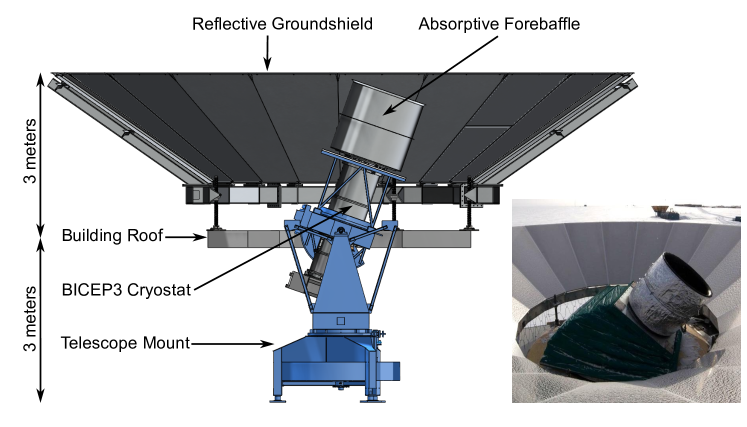
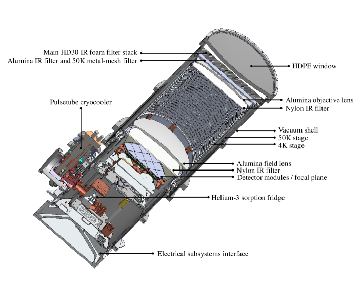
This paper provides an overview of the Bicep3 instrument design and performance with the three-year dataset from 2016 to 2018. Fig. 1 shows the overall layout of Bicep3 as it is installed at the South Pole. The following sections describe the details of each of the subcomponents: telescope mount (§2); optics (§3); cryostat (§4); focal plane unit (§5); transition-edge sensor bolometers (§6); and data acquisition and control system (§7).

Refer to caption — Figure 1: The Bicep3 telescope in the mount, looking out through the roof of the Dark Sector Laboratory (DSL) located $\sim 1100$ m from the geographic South Pole. The insulating environmental shield shown in the bottom right photo is hidden in the CAD layout. The three-axis mount previously used in Bicep1 and Bicep2 allows for motion in azimuth, elevation, and boresight rotation. A co-moving absorptive forebaffle extends skyward beyond the cryostat receiver to intercept stray light outside the designed field-of-view. Additionally, the telescope is surrounded by a stationary reflective ground shield which redirects off-axis rays to the cold sky.

In particular, Bicep3’s 520 mm diameter aperture is $\sim 2$ times the size of the Keck design. This is realized by the large diameter alumina optics shown in §3.1. The increase in aperture size allowed us to accommodate 2400 detectors in the focal plane, compared to 288 detectors in the previous Keck 95 GHz receivers. The new modular focal plane design in §5 allows rapid rework and dramatically reduces risk. The high number of detectors also requires a mature multiplexing readout. Bicep3 is the first experiment to adapt the new generation flux-activated time domain multiplexing system described in §7. Most CMB experiments utilize low temperature, superconducting detectors that operate below 1 K. Rapid development in mechanical compressor cryocoolers allowed ground-based telescopes to phase out the need of liquid Helium, but the high-pressure Helium lines in the system between the telescope and compressor induce significant wear in a continuous rotating mount. We address this by integrating a helium rotary joint into the telescope mount system, allowing for continuous rotation while maintaining a high-pressure seal and electrical connectivity (§2).

The achieved performance characteristics of the receiver and detector properties of Bicep3 are presented in §8, the observing strategy is presented in §9, and in §10 we show the first three-year data set taken from 2016 to 2018, reporting its internal consistency validation, sensitivity, and map depth. The cosmological analysis using Planck, WMAP, and Bicep/Keck observations through the 2018 observing season are presented in BICEP/Keck et al. (2021a).

2 Telescope Mount, Forebaffle and Ground Shield

2.1 Telescope mount

Bicep3 is installed in the Dark Sector Laboratory building, approximately a kilometer away from the South Pole Station. The base of the telescope mount is supported by a platform on the second floor of the building, with a 2.4 m diameter opening in the roof for telescope access to the sky (Fig. 1). The warm indoor environment of the building is extended beyond the roof level by a flexible insulating environmental shield, so that only the receiver window is exposed to the Antarctic ambient temperature.

Bicep3 uses a steel three-axis mount built by Vertex-RSI¹¹1Now General Dynamics Satcom Technologies, Newton, NC 28658, http://www.gdsatcom.com/vertexrsi.php. It was originally built for Bicep1 and also housed Bicep2 until 2013. The mount structure was modified in 2014 to accommodate the larger Bicep3 receiver.

The mount moves in azimuth and elevation, with the third axis rotating about the boresight of the telescope (“deck” rotation). The range of motion of the mount is $48^{\circ}$ to $110^{\circ}$ in elevation and $400^{\circ}$ in azimuth, capable of scanning at speeds of $5^{\circ}$ /s in azimuth. The Bicep3 cryostat houses a pulse tube cryocooler which limits the accessible deck angle to less than a full $360^{\circ}$ rotation in the Bicep mount. However, the design still allows the telescope to scan with two sets of $180^{\circ}$ opposing deck angles, offset from each other by $45^{\circ}$ , retaining an effective set of observation schedules in order to probe systematic errors, as shown in §9.

2.2 Helium rotary joint

The pulse tube cryogenic cooler comprises two sub-systems: a coldhead installed inside the receiver, and a helium compressor located in the building, away from the telescope mount. This pulse tube provides cooling by expanding a high pressure helium gas volume, and requires high and low pressure helium flexible lines to be routed from the compressor, through the three mount axes (azimuth, elevation, and boresight), to the coldhead in the receiver.

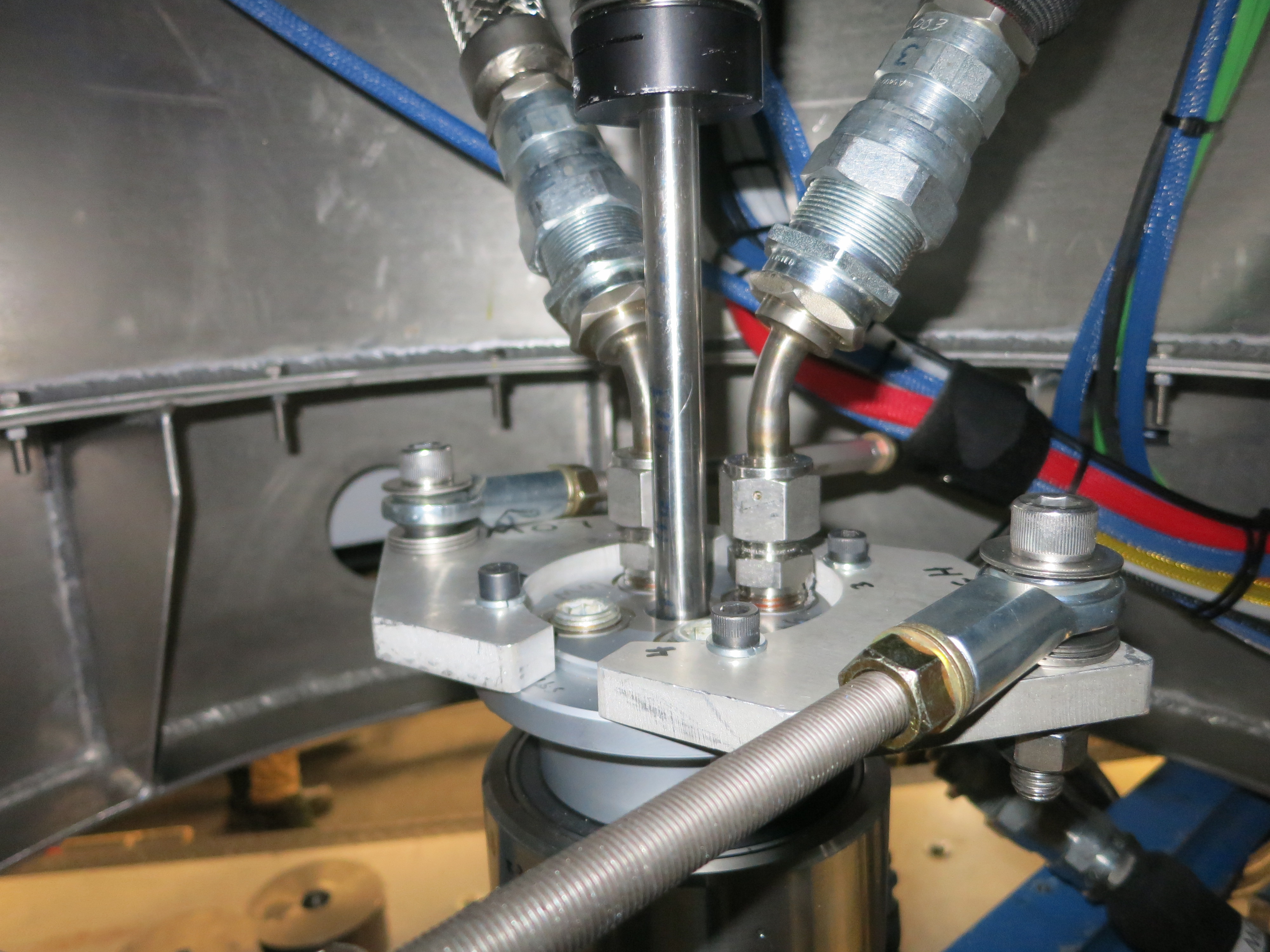
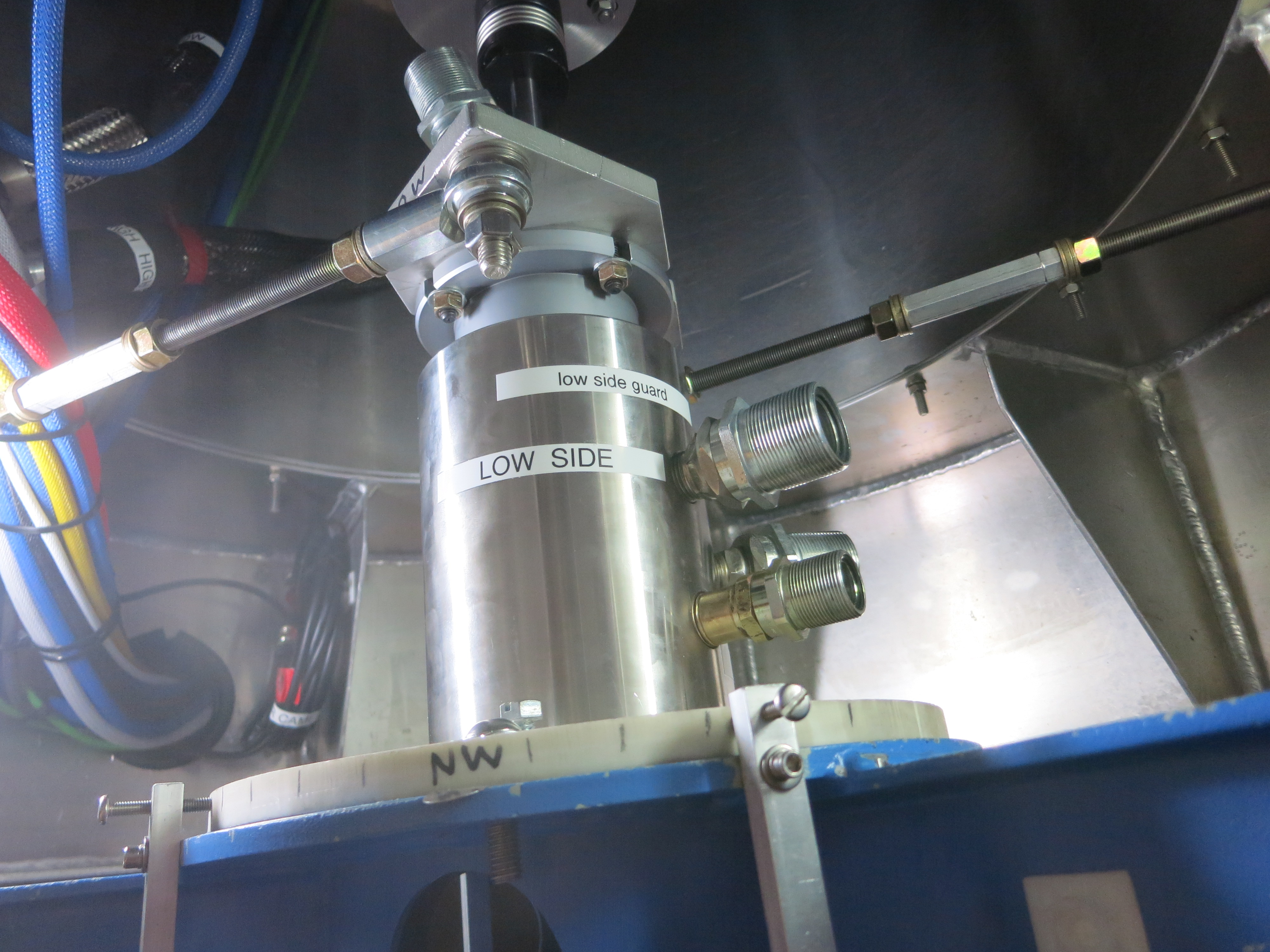
During an observing schedule, movements in elevation and boresight are intermittent and span a limited range of angles, unlike the azimuth axis which scans back and forth continuously in azimuth with a $130^{\circ}$ range. To avoid wear on the compressor lines in the helium line wrap, Bicep3 uses a commercial high-pressure-gas rotary joint from DSTI²²2Dynamic Sealing Technologies, Inc., Andover, MN 55304, www.dsti.com that enables the two pressurized helium gas lines to pass through the azimuth motion. In this joint, shown in Fig. 2, one set of lines remains static at the base of the mount and connects to the helium rotary joint, from which a second set of lines rotate with the azimuth axis of the mount. Therefore the azimuth cable carrier only needs to handle the much more flexible electrical cables.

During the 2015 engineering season, the original design used a basic 2-channel rotary joint (DSTI model: GP-421) to connect the compressor’s high and low pressure helium channels at 290 and 90 PSI, respectively. However, helium gas can permeate materials and gaps much more easily than other larger gas molecules, and this commercial rotary joint was not designed specifically for helium gas. We found the overall system lost 3-5 PSI of pressure per day, originating in the dynamic seals of the rotary joint. Such a large leak resulted in the need to refill the compressor system multiple times a week to maintain optimal pulse tube performance. In addition to being extremely labor-intensive for the telescope operator, these repeated helium refills introduced contamination into the pulse tube, and eventually degraded the cooling performance.

To remedy the high leak rate, the rotary joint was replaced with a 4-channel model (DSTI model: GP-441) before the 2016 season. The 4 channels were configured such that the two working high pressure helium lines would be guarded by two outer channels, serving as pressurized buffers. Thus, the dynamic seals between the two inner high pressure lines would only ‘sense’ the small differential pressure to the pressurized buffers ( $\sim 10$ PSI) instead of the much larger differential to atmospheric pressure ( $>100$ PSI). This configuration reduced the leak rate of the active channels to between $\sim$ 0.1 and 0.5 PSI per day over an entire season³³3The guard channels still have similar leak rate as the 2-channel design, but this is acceptable since refills for them do not affect the pulse tube performance.. The reduced helium leak rate requires less frequent refills, and enables optimal pulse tube performance throughout a full season. The HRJ dynamic seals receive a complete replacement once per year.

2.3 Ground shield and absorptive baffle

A warm, absorptive forebaffle as shown in Fig. 1 extends skyward beyond the cryostat receiver to intercept stray light outside the designed field-of-view. The forebaffle is mounted directly to the receiver and therefore co-moving with the axes of motion of the telescope. The forebaffle is constructed from a large aluminum cylinder, 1.3 m in diameter and height, with a rolled top edge lined by microwave-absorptive Eccosorb HR-10 foam. Heater tape keeps the forebaffle a few degrees above the Antarctic ambient temperature to help avoid snow accumulation, and a layer of closed-cell polyethylene foam (Volara) protects the Eccosorb from accumulating moisture. Based on radiative loading on the detectors observed once the forebaffle is installed, the forebaffle intercepts $\sim 10\%$ of the total optical power. The source of this wide-angle response is likely a combination of scattering and multiple reflections.

Additionally, the telescope is surrounded by a stationary reflective ground shield. It is fixed to the roof of the building to act as a second barrier against stray light and signal contamination from nearby ground sources and reduces the large radiative gradient between the sky and the ground. The ground shield is 10 m in diameter and 3 m in height, constructed with aluminum honeycomb panels and steel beams. The combination of the baffle and the ground shield is designed such that off-axis rays from the telescope must diffract at least twice before intercepting the ground.

2.4 Star camera

An optical camera is used to determine mount pointing parameters (§9.4). It is attached to the side of the receiver vacuum jacket, and looks up through a hole in the bottom of the forebaffle. An optical baffle reduces stray light when using the star camera during daylight and twilight conditions, but is removed for CMB observations. The telescope is a Newtonian reflector, with a 10 cm aluminum-coated⁴⁴4Edmund Optics, Inc., Barrington, NJ, USA objective and a 44 cm focal length. A 700 nm low-pass edge filter removes much of the Rayleigh-scattered sunlight during daylight and twilight. The camera is a CCD with video readout⁵⁵5Astrovid StellaCam Ex, Adirondack Video Astronomy, 72 Harrison Avenue, Hudson Falls, New York, USA; the CCD is a Sony ICX248AL B/W, Sony Group Corporation, 1-7-1 Konan Minato-ku, Tokyo, 108-0075 Japan, and the video-to-digital conversion is done with a video capture card⁶⁶6Sensoray, 7313 SW Tech Center Dr., Tigard, OR, USA in one of the control computers. The field of view is approximately $0.8^{\circ}\times 0.6^{\circ}$ . The CCD is on a linear stage to allow focusing via a remote controller used by the operator.

3 Optics

3.1 Optical design

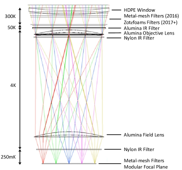
Bicep3 utilizes the same concept as previous Bicep/Keck receivers, using a compact, on-axis, two-refractor optical design that provides a wide field of view and a telecentric focal plane. It has a 4 K aperture of 520 mm and beam width given by a Gaussian radius $\sigma\sim 8.9^{\prime}$ . The lenses and filters operate at cryogenic temperatures inside of the cryostat receiver to minimize excess in-band photon loading. The HDPE plastic cryostat window is at ambient temperature. Thermal filters mounted behind the window cool radiatively. Table 2 shows Bicep3’s optical design parameters compared to previous Bicep/Keck receivers.

Table 2: Optical design parameters for Bicep2 at 150 GHz and Bicep3 at 95 GHz.

	Bicep2/	Bicep3
	Keck
Aperture dia.	264 mm	520 mm
Field of view	15^∘	27.4^∘
Beam width $\sigma$	$12^{\prime}$	$8.9^{\prime}$
Focal ratio	$f/2.2$	$f/1.6$

The ray diagram and full optical chain are shown in Fig. 3. The radially symmetric optical design allows for well-matched beams for two idealized orthogonally polarized detectors at the focal plane.

3.2 Vacuum window and membrane

The first optical element in the receiver is the vacuum window. Bicep2/Keck used laminated Zotefoam⁷⁷7Plastazote HD30 from Zotefoams, Inc., Walton, KY 41094, USA, www.zotefoams.com (Zotefoam HD30), but Bicep3 instead uses a 31.75 mm thick, 73 cm diameter high-density polyethylene (HDPE) window due to the larger aperture setting more stringent requirements on its mechanical strength. The surfaces of the HDPE window are coated with a $\lambda/4$ anti-reflective (AR) layer made of Teadit 24RGD⁸⁸8TEADIT North America, Pasadena, TX, USA (expanded PTFE sheet). The AR coating adheres to the window with a thin layer of low-density polyethylene (LDPE) plastic, melted in a vacuum oven press.

In front of the window is a 22.9 $\mu$ m thick biaxially oriented polypropylene (BOPP) membrane to protect the window from snow and create an enclosed space below, which is slightly pressurized with room temperature nitrogen gas to evaporate snow that falls onto the membrane surface.

3.3 Large-diameter 300 K filters

Inside the receiver and directly behind the vacuum window is a set of infrared filters to reduce the thermal loading in the receiver. These are a stack of 10 thin filters mounted on a set of aluminum rings mechanically connected to the room-temperature vacuum jacket. The filters reflect or absorb infrared radiation in stages, and radiatively equilibrate at progressively lower temperatures to reduce the thermal infrared power into the cryostat.

The original design used a set of metal-mesh filters, composed of 3.5 µm Mylar or 6 µm polypropylene/polyethylene (PP/PE) film, pre-aluminized to a 40 nm deposition thickness and laser ablated to form a grid of metal squares (Ahmed et al., 2014). However, we found that the performance of the metal-mesh filter depended on the etching process of the metal on the thin film, and minor defects in fabrication introduced excess in-band scattering from the filters. The in-band scattering was slightly polarized, leading to additional mm-wave power on the detectors, and associated photon noise. Furthermore, simulations using high-frequency structure simulator (HFSS⁹⁹9Ansys, www.ansys.com) software indicated of order 0.5% specular reflection per layer even without defects.

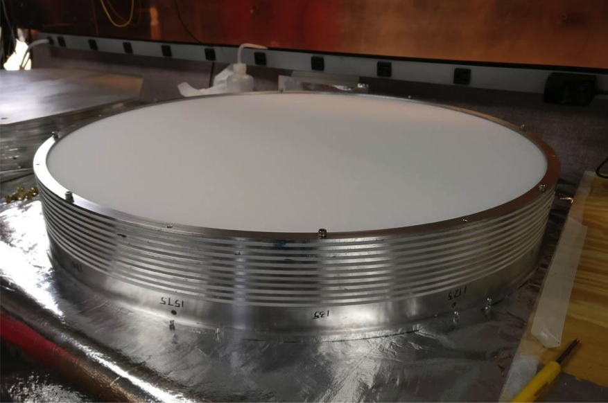
All the metal-mesh filters except for one placed behind the 50 K alumina filter were replaced in 2017 with a set of ten, 3.17 mm thick Zotefoam layers (Fig. 4). These filters are nitrogen-expanded polyethylene foam layers that scatter infrared radiation (IR) isotropically and therefore act as floating radiative layers, while maintaining $>$ 99 % transmission in-band. Using room-temperature transmission measurements, we estimate 8 % improvement in-band transmission compared to the metal-mesh filters. Table 3 details the individual filters used in Bicep3.

Table 3: Room temperature IR filters installed in Bicep3. The main stack of 10 filters behind the window are listed in order beginning with the closest filter to the window. The metal-mesh filters were replaced by Zotefoam in 2017.

	2016	Square/pitch	2017+
Location	Substrate	[ $\mu$ m]	Substrate
Behind window	3.5 $\mu$ m Mylar	50/80	HD-30 foam
( $\sim 290$ K)	3.5 $\mu$ m Mylar	40/55	HD-30 foam
	3.5 $\mu$ m Mylar	50/80	HD-30 foam
	3.5 $\mu$ m Mylar	40/55	HD-30 foam
	3.5 $\mu$ m Mylar	90/150	HD-30 foam
	6 $\mu$ m PP/PE	40/55	HD-30 foam
	3.5 $\mu$ m Mylar	50/80	HD-30 foam
	3.5 $\mu$ m Mylar	40/55	HD-30 foam
	3.5 $\mu$ m Mylar	50/80	HD-30 foam
	3.5 $\mu$ m Mylar	90/150	HD-30 foam
Behind 50 K	3.5 $\mu$ m Mylar	90/150	3.5 $\mu$ m Mylar
Alumina filter

3.4 Alumina thermal filter and optics

Motivated by the larger aperture diameter and faster $f/1.6$ speed in Bicep3, we developed large-diameter alumina filters and their anti-reflection coating. Alumina lenses are much thinner and less-aggressively shaped than their HDPE equivalents owing to the significantly higher index of refraction at $n=3.1$ . The alumina optics are 21 mm and 27 mm thick at the center for the field and objective lens respectively, compared to $>67$ mm for a comparable HDPE design. Both the lenses and 50 K filter are made from 99.6% pure alumina sourced from CoorsTek¹⁰¹⁰10CoorsTek, Golden, CO 80401, USA, www.coorstek.com.

The reduction in thickness and high thermal conductivity of alumina ( $0.5\ \text{Wm}^{-1}\text{K}^{-1}$ at 4 K) enables the optical elements to cool to base temperatures more rapidly and limits any thermal gradient across the lenses to less than 1 K from center to edge. Lab measurements of similar alumina materials indicate low in-band absorption at room temperature which decreases with temperature (Penn et al., 1997; Inoue et al., 2014). Our own measurements at room temperature indicated significant differences between various formulae, and the CoorsTek AD-996 Si used for the filter and lenses was the best we tested. After deployment, we also confirmed substantially decreased loss at 77 K. A single 10 mm thick alumina disk serves as an absorptive thermal filter, mounted on the 50 K cryogenic stage. The high mid-IR absorption and high thermal conductivity make alumina a choice material for this application.

The AR coating used for the alumina optics is a mixture of Stycast 1090 and 2850FT with a homogeneous refractive index of $n=1.74$ . The epoxy is poured and rough-molded to 1 mm thickness on the alumina surface, then either machined (lenses) or abrasively ground (flat filter) to the final 0.452 mm thickness. The thickness of the coating is controlled to less than 25 µm tolerance by referencing pre-coating surface measurements of the alumina.

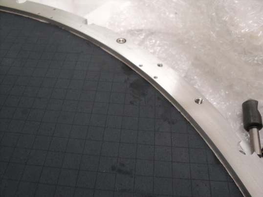
Historically, alumina optics were limited to small sizes unless accommodation for differential contraction between the alumina and the epoxy was made. Inoue et al. (2014); Rosen et al. (2013) put slices through their coatings to allow cryogenic operation. We adopted a laser cutting technique using Laserod¹¹¹¹11Laserod Technologies LLC, Torrance, CA 90501, USA, the same commercial laser machining company that etched the IR blocking metal-mesh film filters described above. The laser cuts in the AR epoxy are $\sim 30\mu$ m wide, tuned to reach the alumina surface, and spaced every 10 mm in a square grid pattern (Fig. 5).

3.5 Nylon IR blocking filters

Following the same machining and coating approach in Bicep2/Keck (BICEP2 collaboration et al., 2014b), two Nylon IR blocking filters are placed in the receiver. One is behind the aperture stop; the other is behind the field lens, above the focal plane (FPU) assembly, both at 4 K. Nylon strongly absorbs far-infrared radiation (Halpern et al., 1986) and thus reduces radiated power from 50 K from reaching the 280 mK focal plane.

3.6 Metal mesh low-pass edge filters

A set of metal mesh low-pass edge filters (Ade et al., 2006) with a cutoff at 4 cm^-1 were used to control any out-of-band response in the detectors. They are made from multiple polypropylene substrate layers, each coated with copper grids in different sizes, and hot-pressed together to form a resonant filter.

Prior to the 2017 season, these filters were cut into 76 mm $\times$ 76 mm squares and independently mounted onto each detector module (§5) at 280 mK. We found anomalous detector spectral responses in the 2016 FTS measurements described in §8.1. Upon examining the filters at the end of the 2016 season, we found the layers had delaminated. It was determined that the cause of delamination was likely insufficient oven temperature during fabrication. Furthermore, the cutting of individual, smaller filters introduced extra stress on the edge contributing to the delamination.

New filters were fabricated using a higher oven temperature in the fusing process. The filter design was modified to a larger $\sim$ 23 cm $\times$ 15 cm size covering 5 detector modules. This change reduced mechanical stress at the filter edges caused by the dicing process. Extra spring loaded washers and widened mounting slots allowed the filter to slide more freely during thermal contraction. These modifications were done at the end of the 2016 season and subsequent FTS measurements showed no evidence of filter delamination.

3.7 Optical loading reduction

The dominant noise source in Bicep3 is the photon noise of the in-band signal power. For better sensitivity, it is important to minimize the internal non-sky instrument load.

We calculated the total internal loading by measuring the detector responsivity with a flat aluminum sheet mounted just beyond the cryostat window (procedure describe in §8.2). The detector beams were reflected and therefore received power only from within the cryostat. The co-moving forebaffle loading is measured by differencing of the detector response with and without the forebaffle during clear weather while looking at zenith.

The optical power coupled to the detectors due to each individual optical element is calculated by using the transmission properties of the material and finding the source temperature distribution. The calculation incorporates the cumulative optical efficiency from the detector up to the source, and includes the emissivity of the source itself. For the 2016 design, a simple scattering model is used for the room temperature metal-mesh filters, in which each filter isotropically scatters a small fraction of the radiation to wide angles and warms surfaces around them. Table 4 shows the modeled in-band loading estimate for each individual elements and the total measured loading. The agreement between them validates the model assumption.

A significant contributor to the cryostat internal loading was the scattering of the metal-mesh IR-reflective filters before their replacement in 2017 with the Zotefoam filters. The reduction of scattered radiation coupling to the filters and telescope forebaffle results in a decrease of the total instrument loading by 30%.

Non-sky loading also comes from the room temperature HDPE cryostat window, which now dominates the internal power. We are developing thinner materials that can potentially replace the window in future seasons (Barkats et al., 2018).

Table 4: Per-detector in-band optical load. The total loadings listed in bold are direct measurements from detector load curves, which are in good agreement with the individual modeled optical elements. A stack of 300 K metal-mesh filters used in the 2016 season were replaced by HD-30 foam filters for the 2017 season.

Source	Load [pW]	$T_{\mathrm{RJ}}$ [K]
4K lenses & elements	0.15	01.0
50K alumina filter	0.12	00.9
Metal-mesh filters (2016)	0.63	05.2
HD-30 foam filters (2017+)	0.10	00.8
Window	0.69	05.9
Total cryostat internal (2016)	1.60	13.0
Total cryostat internal (2017+)	1.10	08.6
Forebaffle (2016)	0.31	02.7
Forebaffle (2017+)	0.14	01.1
Atmosphere	1.10	09.9
CMB	0.12	01.1
Total (2016)	3.13	27
Total (2017+)	2.46	21

4 Cryostat receiver

4.1 Overview

The cryostat receiver is a compact, cylindrical design that allows for a large optical path while maintaining sub-Kelvin focal plane temperatures (Fig. 6). The fully populated receiver weighs about 540 kg without the attached electronics subsystems. The outermost aluminum vacuum jacket is 2.4 m tall along the optical axis and 73 cm in diameter, excluding the pulse tube cryocooler extension. It maintains high vacuum for thermal isolation and is capped at one end by the HDPE plastic window, as described in §3.1.

The wide-field refractor design allows for ground-based characterization in the optical far field. The optical design further allows the use of a co-moving, absorptive forebaffle (§2.3) that terminates stray light and wide angle response from the receiver. Cooling most of the optical elements, including the internal baffling between the lenses, to less than 4 K reduces the thermal photon noise seen by the detectors, maximizing the sensitivity of the instrument.

4.2 Cryogenic and thermal architecture

Nested within the room-temperature vacuum jacket are the 50 K and 4 K stages, each comprised of cylindrical aluminum radiation shields and cooled by the 1^st and 2^nd stages of the PT-415 pulse tube cryocooler¹²¹²12Cryomech Inc., Syracuse, NY 13211, USA (www.cryomech.com), which provides continuous cooling to 35 K at the ‘50 K stage’ under typical 26 W load and 3.3 K at ‘4 K stage’ under 0.5 W load. The stages are mechanically supported off each other and the vacuum jacket by low thermal-conductivity, G-10 fiberglass. Multi-layer insulation (MLI) wrapped around radiation shields minimizes radiative heat transfer between the 300-50-4 K stages.

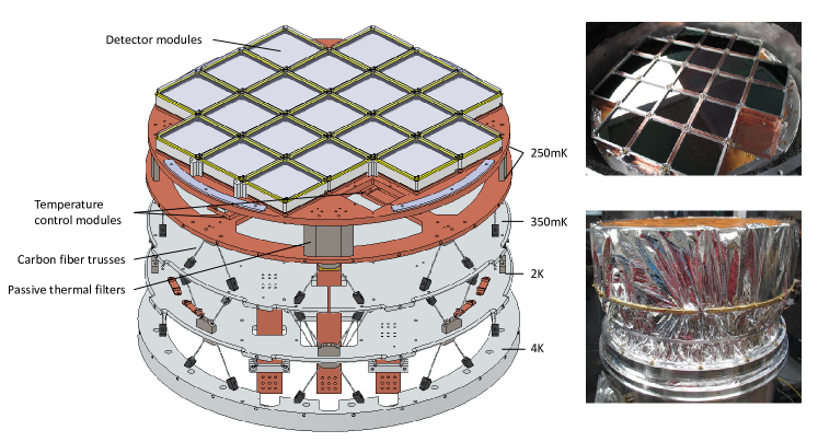
A non-continuous, three-stage (⁴He/³He/³He) helium sorption fridge from Chase Research Cryogenic¹³¹³13Chase Research Cryogenics Ltd., Sheffield, S10 5DL, UK (www.chasecryogenics.com) is heat sunk to the 4 K stage and cools the sub-Kelvin focal plane and supporting structures. The focal plane and ultra-cold (UC 250 mK) stage is a planar copper assembly mounted in a vertical stack on two buffer stages, the inter-cooler ³He (IC 350 mK) and ⁴He (2K) stages, each supported and isolated by carbon fiber trusses (Fig. 7). The UC stage cools a 9 mm thick, 46 cm diameter focal plane plate that supports the detector modules and a thinner secondary plate. These plates are made from gold-plated, oxygen-free high thermal conductivity (OFHC) copper. The secondary plate and the focal plane are separated by seven 5 cm tall stainless steel blocks that serve as passive low-pass thermal filters to dampen thermal fluctuations to the focal plane. The focal plane and the UC stage are actively temperature controlled in a feedback loop to 274 mK and 269 mK, respectively, using Neutron transmutation doped (NTD) Germanium thermometers and a resistive heater. Thermal fluctuations on the focal plane during CMB observation are controlled to $<0.1$ mK.

4.3 Thermal performance

The sum of all incident thermal power on the 50 K and 4 K stages determines the temperature profile of the elements along each stage and the base operating temperature of the pulse tube.

The room-temperature HDPE plastic window emits $\sim$ 110 W of power into the receiver while the pulse tube cryocooler is rated for less than 40 W on the 50 K stage. We employed two different types of thermal filters at 300 K mounted just behind the cryostat window to reject the majority of the IR load: (1) a stack of thin film, IR-reflective, capacitive metal-mesh filters in 2016; and (2) a stack of Zotefoam filters starting in 2017. The reason for switching the design is discussed in §3.3.

An alumina filter is heatsunk to the 50 K stage, to provide absorptive IR filtering due to Alumina’s mid-infrared absorption and high thermal conductivity. This replaced the filters used in previous telescopes. Two additional nylon filters are placed in the 4 K stage of the receiver to reduce thermal loading on the sub-Kelvin focal plane by absorbing infrared radiation. Table 5 shows the final temperature and power deposited onto each cryogenic stage. Switching from metal mesh filters to Zotefoam filters in 2017 reduced the thermal loading and improved the cryogenic hold time of the sub-Kelvin fridge from $\sim 50$ to $>80$ hours, with 6 hours of recycling time. This permits the continuous three-day observation schedule shown in §9.2.

Table 5: Measured final temperature and thermal loading on each temperature stage in Bicep3.

	2016	2017+
Stages	Temp/Load	Temp/Load
50 K tube top	58 K	53 K
50 K tube bottom	52 K	49 K
50 K tube loading	19 W	13 W
4 K tube top	4.96 K	4.68 K
4 K tube bottom	4.58 K	4.33 K
4 K tube loading	0.18 W	0.15 W
350 mK stage	354 mK	352 mK
250 mK stage	245 mK	244 mK
Focal Plane	268 mK	268 mK

4.4 Cryogenic thermal monitoring and control

For general thermometry down to 4 K, we use silicon diode thermometers (Lakeshore¹⁴¹⁴14Lake Shore Cryotronics, Westerville, OH 43082, USA (www.lakeshore.com) DT-670), with thin-film resistance temperature detectors (Lakeshore Cernox RTDs) on the sub-K stages. NTD Germanium thermometers are integrated in the secondary UC stage, copper focal plane, and each detector module for more sensitive measurements of the temperatures. The NTDs on the secondary UC stage and focal plane are packaged with a heater to provide active temperature control on their respective temperature stages.

Thermal operations are controlled by a custom-built system similar to the one used in Bicep2/Keck. It contains electronic cards used to bias and read out thermometers, control heaters and provide temperature control servos, and is mounted directly to the cryostat vacuum jacket and interfaces with MicroD (MDM) connectors¹⁵¹⁵15Glenair Inc., Glendale, CA 91201, USA (www.glenair.com) at the cryostat. Signals from the system are routed to the rack-mounted BLASTbus ADC system (Wiebe, 2008) next to the telescope which generates the AC bias used for the resistive thermometers and the NTDs, and demodulates the thermometer signals, which are then digitized at $\sim$ 100 Hz.

4.5 Radio frequency shielding

Several levels of radio frequency (RF) shielding are designed into the 4 K stage and sub-Kelvin structures to minimize RF coupling to the detectors. All cabling inside the cryostat uses twisted pairs, except for the short lengths of flex ribbon cable connecting the detector modules to the focal plane readout circuit board. These ribbon cables are shielded by the detector module, copper focal plane module cutout, and the ground plane of the circuit board that accepts the cable. The 4 K non-optics volume is designed as a Faraday enclosure, with all seams taped with conductive aluminum tape and cabling passing through inductive-capacitive PI-filtered connectors¹⁶¹⁶16Cristek Inc., Anaheim, CA 92807, USA (www.cristek.com). The cage is continued to enclose the stack of sub-Kelvin stages by wrapping and sealing a single layer of aluminized mylar between the 4 K stage and the edge of the focal plane. The niobium enclosure of each detector module and detector tile ground plane close the sky side of the Faraday cage. Upon exiting the cryostat, all of the detector signal lines immediately interface with a capacitive filtered connection on the readout electronics box that is directly mounted on the cryostat.

During the 2015 engineering season, we found an azimuth-synchronous signal strongly affecting the detectors, largely common-mode across a large fraction of detectors within each readout system. These interference showed variation 1000 times larger than the $50\mu$ K CMB temperature variations, causing ‘SQUID jumps’ because of the strong signals. Our detector readout scheme works through feedback to maintain linearity in the SQUID amplification curve (§7.1), but large current variations can disrupt the feedback and cause the readout to jump to a different part of the SQUID curve. We discovered that this interference signal was caused by radio-frequency emission from the South Pole station land mobile radio (LMR) system at 450MHz, coupling into the cryostat and detectors through the cryostat window. Bicep3 is inherently more susceptible to this 450 MHz signal than Keck due to its larger aperture, which has a cutoff frequency at 340MHz at the optics cylinder.

Prior to the 2016 season, we applied silver loaded paste between the detector modules and copper focal plane, so that reliable electrical conductivity was maintained from the modules to the focal plane. In 2015, only 9 out of 20 detector modules were filled, leaving large gaps at the top of the focal plane. In 2016, having the full population of 20 detector modules provided a better RF shielded enclosure. After implementing the improved internal cryostat shielding, RF susceptibility in the range of 400–500MHz was reduced by 10 dB. In addition, the LMR antenna was changed to a directional sector antenna with reduced power output towards the telescope. Attenuators were also installed to reduce the overall broadcast power, which was tested to be much more powerful than necessary to maintain radio communication across the base. In total, the LMR source power seen at the telescope was reduced by 35 dB. Azimuth scanning tests conducted after these changes have shown none of the visible structure seen in 2015.

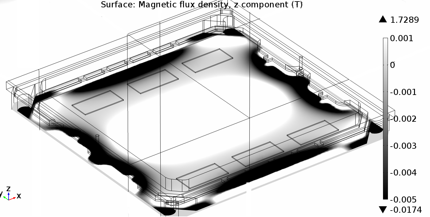
4.6 Magnetic shielding

Earth’s magnetic field ( $\sim 50\mu$ T) is the most dominant variable magnetic environment. While this azimuth-fixed signal is largely filtered out during analysis, instrumental magnetic shielding is crucial to minimize coupling to the TES detectors and the SQUID amplifiers. We incorporate two methods of shielding in the cryostat. First we use a cylindrical, high-permeability Amumetal-4K (A4K)¹⁷¹⁷17Amuneal Manufacturing Corp., (www.amuneal.com/) structure, with open ends to avoid interference with the optics and allow data cabling through the bottom. It is a split shield on the inner surface of the vacuum jacket of the cryostat. The two halves overlap midway, near the focal plane level given the constraints of the cryostat and optics. Additionally, a shorter, superconducting Niobium cylinder is mounted on the 4 K stage, surrounding the focal plane. Lab tests showed a shielding factor of $\sim$ 30 for the magnetic field amplitude along the cylindrical axis of the cryostat.

The detector module, which includes layers of niobium, aluminum and high- $\mu$ A4K (§5.1), provides further shielding of the first-stage SQUID amplifier chips on the sub-Kelvin focal plane. The series SQUID array (SSA) on the 4 K stage are packaged in niobium boxes and additionally wrapped with 10 layers of high- $\mu$ Metglas 2714A¹⁸¹⁸18Metglas Inc., (www.metglas.com). Overall, Bicep3 shows an induced response $\sim$ 7 $\mu\text{K}_{\text{CMB}}/\mu$ T, or 350 $\mu\text{K}_{\text{CMB}}/B_{Earth}$ by directly measuring the SQUID amplifier response to a Helmholtz coil.

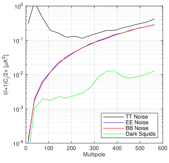
Another method to estimate impact on external magnetic field to the data is using the dark SQUID channels in the readout system (§7.1). These channels are connected to the SQUID amplifiers, but not the detectors, hence ideally only respond to external magnetic fields as the telescope scans. Lab measurements show the properties and calibrations of these dark SQUID channels are similar to the other SQUID channels in the same SQUID chip. Then using the neighboring optical channel calibrations and telescope pointing, we constructed ‘maps’ of these dark SQUIDs. Comparing these maps and the associate spectrum with single optical channel maps, we found the dark SQUID responses are factor of 2 to 20 smaller than the Q/U noise of the same bins (Fig. 8).

5 Focal Plane

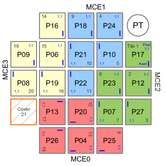
Bicep3 has 2400 detectors, a factor of 9 greater than a single Keck receiver at the same frequency. The detectors are fabricated on 20 silicon wafers, each consisting of 60 dual-polarized detector pairs. Each wafer is packaged into a focal plane module with its cold readout electronics and installed onto the copper focal plane to form the Bicep3 focal plane (Fig. 9). The focal plane base plate provides the necessary thermal stability, magnetic shielding, and mechanical alignment to operate the detectors. The modular design allows individual detector tiles to be replaced with minimum impact to the rest of the receiver.

5.1 Modular packaging

Each detector module is $79\times 79\times 22$ mm in size (Fig. 10). Two 60-pin, 0.5 mm pitch flex ribbon cables connect between each module and the focal plane circuit board, via a pair of zero-insertion force (ZIF) surface-mount connectors. The module mounts on the focal plane on all four corners.

The detector module consists of a quartz anti-reflection coating, detector tile, niobium (Nb) $\lambda/4$ backshort, A4K magnetic shield, and alumina and PCB readout circuit boards. These sub-components are stacked together on the aluminum detector frame, secured at the corners with commercially available copper clips¹⁹¹⁹19Ted Pella Inc., (www.tedpella.com), and aligned with a 2 mm diameter copper pin-slot pairs located on opposing edges of the wafer. The module is enclosed with a niobium housing, an external niobium magnetic shield covering the ribbon cables, and a copper heatsink.

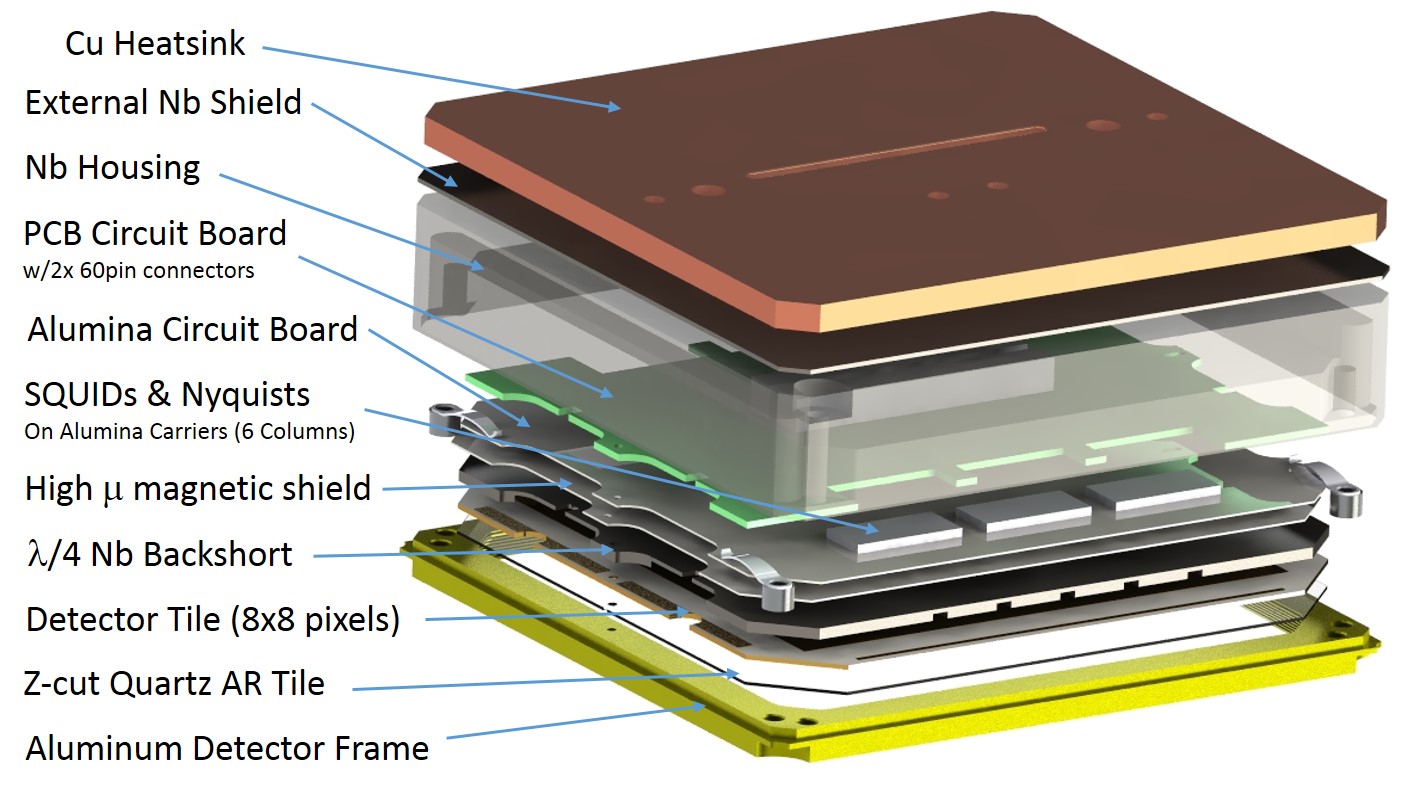
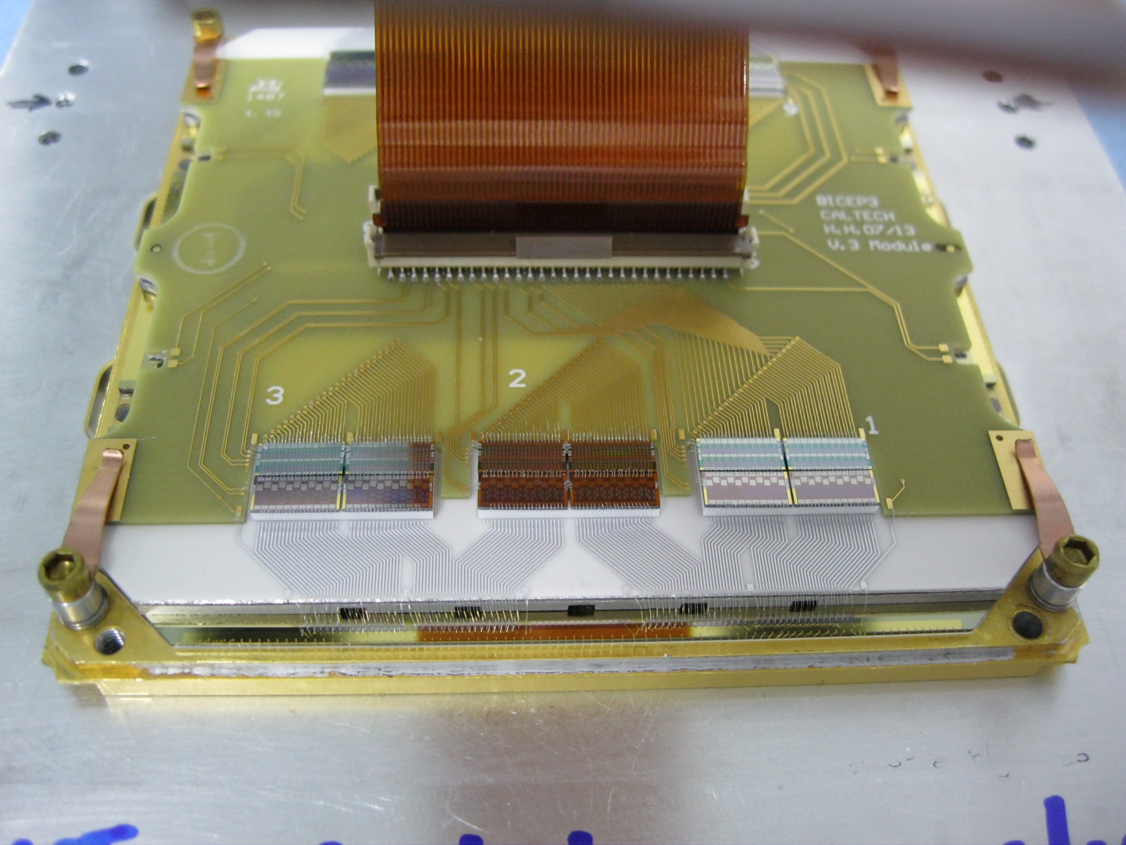
The readout circuit boards are composed of an alumina and a FR4 printed circuit board. The 0.25 mm thick alumina circuit board has 0.13 mm wide, 0.23 mm pitch aluminum traces, creating a superconducting path between the detectors and the SQUID chips. Twelve readout SQUID and Nyquist chips are mounted onto individual alumina carriers which are glued onto the alumina circuit board. On top of the alumina board is a two-layer FR4 circuit board with standard copper traces. These components are electrically connected to each other with aluminum wire bonds, and two 60-pins surface mount connectors are soldered on top of the FR4 circuit board for the flex cables shown in Fig. 11.

5.2 Thermal sinking and magnetic shielding

The detector tiles are thermally sunk to the aluminum frame on all four sides with $\sim$ 500, 0.5 mm pitch gold wirebonds. Additionally, these wirebonds form the top RF shield of the system by connecting the aluminum frame and detector Nb ground plane.

The detector module is mounted to a copper heat-sink at the back of the niobium housing. It is supported by 3 thermally isolated alumina spacers in the corners, making the center-most point the only point of thermal contact between the copper and niobium. This single contact point cools the module housing from the middle, ensuring that the niobium superconducting transition begins from the center and continues radially outwards, avoiding trapped magnetic flux during cool-down.

The backside of the module is completely enclosed with a Nb housing, with only a $35$ mm $\times 1.3$ mm slit to allow the flex cables to exit the module. A 0.5 mm-thick Nb sheet with an offset slit is placed at the back of the housing, creating a near continuous superconducting magnetic shield. Additionally, a sheet of high-permeability Metglas 2714A is placed 1.27 mm away from the SQUID chips inside the module to create the lowest magnetic field environment at the location of the SQUID chips (Fig. 12).

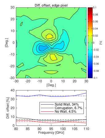
5.3 Corrugated frame

The interaction between the detector module metal frame and the edge-adjacent planar slot antenna causes differential pointing within that detector pair. Although most of the systematic errors caused by the differential pointing are mitigated during analysis, we corrugated the frame to minimize residual beam systematics of these pixels.

The corrugated frame has $\lambda/4$ depth and pitch, and is placed $\lambda/2$ away from the closest antenna, where $\lambda$ is the design band center (Soliman et al., 2018). Fig. 13 presents a differential beam map model using CST Studio Suite²⁰²⁰20Dassault Systemes (www.3ds.com), showing a reduction in residual beam mismatch from $\sim$ 34% with a flat frame to $\sim 6.7\%$ with the corrugated frame, evaluated over the 25% spectral bandwidth.

6 Detectors

Bicep3 inherits the planar phased-array antenna and transition-edge sensor (TES) bolometer detector technology from Bicep2/Keck (Ade et al., 2015). The planar antenna design does not require feed horns or similar coupling optics to free space. The 95 GHz band is defined by lumped-element filters along the microstrip feed line to the bolometers. Each silicon detector tile contains an 8 $\times$ 8 array of pixels and each pixel is made of two co-located, orthogonally-polarized sub-antenna networks and two TES bolometers.

Holding the edge taper on the pupil fixed, Bicep3’s faster focal ratio enables a denser detector packing than the 6 $\times$ 6 array of pixels in each 95 GHz Keck detector tile.

The TES detectors are voltage-biased, providing electro-thermal stability and linearity, where electrical power compensates for variation in optical power. Each TES is made up of a titanium and aluminum film in series; the titanium transition maximizes sensitivity ( $T_{c}\approx 0.5$ K) during normal science observation, while the higher $T_{c}\approx 1.2$ K aluminum TES provides higher saturation power to observe high-temperature calibration sources, though at reduced sensitivity.

Together, the two independent signals from the co-located orthogonal antenna and bolometer pairs on each pixel can be summed to get total incident power or differenced to measure polarization in the vertical-horizontal direction.

6.1 Tapered antenna networks

Optical radiation couples to the detectors through a planar phased antenna array, combined in phase with a summing network that controls the amplitude and phase in each sub-slot. The illumination pattern is controlled through the microstrip feed network that sums signals from the sub-antennas to deliver power to the TES bolometer. Previous designs, used in Bicep2/Keck and Spider, drive each of the sub-antennas in phase with equal field strength, synthesizing a top-hat illumination and thus a sinc pattern in the far field. Such a pattern has side-lobes with peak levels at -13 dB below the main lobe. In these instruments, side-lobes are terminated onto the 4 K aperture stop with limited impact on the sensitivity.

Programmatically, some optical designs would benefit from lower side-lobe levels and Bicep3 was used to advance this capability. The side-lobe levels of antenna arrays can be controlled by tapering the illumination such that the central sub-slots have higher coupling than those at the edge. The array factor with non-uniform illumination can be generalized as

	$\displaystyle A(\theta)$	$\displaystyle=$	$\displaystyle\sum_{m=-(N-1)/2}^{(N-1)/2}E_{m}e^{-jmk\sin(\theta)s}$		(1)
		$\displaystyle\simeq$	$\displaystyle\int_{S}E(x^{\prime},y^{\prime})e^{j(k_{x}x^{\prime}+k_{y}y^{\prime})}\,dx^{\prime}dy^{\prime}$		(1)

where the last line approximates the sum as an integral across the antenna aperture, and $k_{x}$ and $k_{y}$ are the components of the tangential free-space wavevector $k\sin(\theta)$ . This expresses the far-field antenna pattern as the Fourier transform of the illumination pattern. For Bicep3, the feed network was designed to generate a Gaussian illumination with an electric field waist radius of 6.3 mm, compared to the physical aperture size of 7.5 $\times$ 7.5 mm. This reduces the side-lobe levels to -16 dB and the integrated spillover to 13% compared to the 17% that would have been achieved with a uniform feed. The result is an illumination that is close to uniform, as the instrument’s aperture stop requires, but also allows our team to develop flexibility for other instruments. We also developed and tested two designs with stronger tapering, which would be advantageous in optical systems with a warm pupil stop.

7 Data Acquisition system

Bicep3 uses a SQUID time-division multiplexed (TDM) system for the bolometer readout, which includes the SQUID multiplexing chips, the room temperature Multi-Channel Electronic (MCE) system and the overall Generic Control Program (GCP).

7.1 Time-division multiplexing SQUID readout

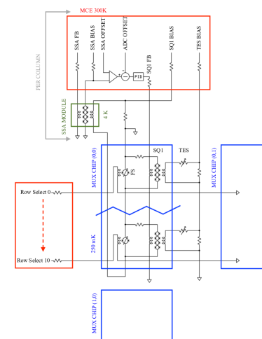
Bicep3 uses a low-noise SQUID TDM readout system, which amplifies the small current flowing through the TES while adding noise sub-dominant to the detector itself, and transforms the small $\sim 60$ m $\Omega$ impedance of the TES in two amplification stages. The TDM architecture is similar to previous experiments (de Korte et al., 2003) but uses a new generation MUX11 model that takes advantage of superconducting-to-resistive, flux-activated switches (FS) in the multiplexing sequence (Irwin et al., 2012). The SQUID amplifier chips were developed and fabricated by National Institute of Standards and Technology (NIST), and the operating firmware and characterization were first demonstrated in Bicep3 (Hui et al., 2016). Since then the technology has been deployed in Advanced ACTPol (Henderson et al., 2016), CLASS (Dahal et al., 2020) and Bicep Array (Hui et al., 2018).

In the readout architecture each independent detector is inductively coupled to a single SQUID array (SQ1) by an input coil, and the amplifier is operated in a flux-lock loop to linearize the output and increase the dynamic range of the periodic SQUID response. As the flux from the input coil changes in response to the TES current, a compensating flux is applied by the feedback coil to cancel it. This flux feedback serves as the signal output of the TES. The second stage SQUID array (SSA) at 4 K provides additional amplification that impedance matches to the room temperature MCE, providing $\sim 1\Omega$ dynamic resistance and a $\sim 100\Omega$ output impedance.

The multiplexing circuit is arranged according to ‘columns’ and ‘rows’ of detectors. Bicep3 uses total of 4 MCE, each MCE readout 660 channels, which are mapped into 30 MUX columns and 22 MUX rows (600 optical channels, 20 dark detectors, and 40 dark SQUID channels.) Multiplexing is done across rows, such that 22 channels of each column are read out in TDM sequence. The SQ1 on each column lie in series, and the entire line is resistively shunted by the FS. The FS are a four-Josephson-junction design that behaves like a SQUID with a critical current about twice the critical current of the SQ1 when no flux is applied to them. The SQ1 and FS are shared by the same SQ1 bias line; a zero flux applied to an FS leaves it superconducting, while half of a flux quantum applied sends the FS normal with a resistance much greater than SQ1. Each FS is coupled to an input inductor, which can apply a flux and is driven by a row-selected input line (RS) which runs across columns. At a given moment in time during the multiplexing sequence, only one RS line applies a half flux quantum to the switches of its row, while the remaining 21 RS lines remain zeroed, resulting the shared SQ1 bias current shorts through those 21 FS. This bypasses those SQ1s and only flows through the single SQ1 whose FS is highly resistive. The circuit diagram of the TDM system is shown in Fig. 14.

Additionally, the TES bias circuits includes elements of a ‘Nyquist’ chip (NYQ), which consists of a shunt resistor $R_{sh}\sim 3$ m $\Omega$ parallel to the TES, and an inductor $L_{\text{NYQ}}$ in series with the TES. The inductor is included to create a RL filter with the TES resistance, with $L_{\text{NYQ}}\sim 2\mu$ H, $R_{\text{TES}}\sim 50$ m $\Omega$ resulting a roll off at $\sim 4$ kHz to avoid aliasing of higher frequency noise.

7.2 Warm multiplexing hardware

Control of the MUX system and feedback-based readout of the TES data are done via the room temperature MCE system (Battistelli et al., 2008).

The MCE samples the raw SSA output at 50 MHz, givens a 90 samples each row in the MUX sequence per switch. This gives a 25.3 kHz visitation rate. The data are filtered and downsampled in the MCE before being output to the control system. The MCE uses a fourth-order digital Butterworth filter before downsampling by a factor of 168, then the the final electronic stage applies a second filtering using an acausal, zero-phase-delay finite impulse response (FIR) low-pass filter, down-sampled by another factor of 5, giving an archived sample rate of 30.1 Hz. The full multiplexing parameters used in Bicep3 are shown in Table 6.

Table 6: Summary of multiplexing readout parameters used by Bicep3.

Raw ADC sample rate	50 MHz
Row dwell	90 samples
Row switching rate	556 kHz
Number of rows	22
Same-row revisit rate	25.3 kHz
Output data rate per channel	150 Hz
Archived data rate	30.1 Hz

7.3 Control system

All of the telescope systems are controlled and read out by a set of six Linux computers running GCP, inherited and modified from Bicep/Keck and other CMB experiments (Story et al., 2012). These control computers interface with all telescope subsystems, including mount movement control, detectors and SQUIDs via the MCEs, and thermometry. All data timestreams are packaged into archived files on disk and streamed back with telescope operation logs to North America via daily satellite uplink. Observation and fridge-cycle scheduling are scripted within GCP and executed automatically with periodic monitoring by the operator.

8 Instrument characterization

8.1 Detector bands

Bicep3 detectors are designed for a frequency band centered at 95 GHz with $\sim 25\%$ fractional bandwidth. The band is chosen to avoid the broad oxygen absorption band around 60 GHz as well as the oxygen spectral line at 118.8 GHz.

The spectral response of each detector is measured in situ with a custom-built Martin-Puplett Fourier Transform Spectrometer (FTS) mounted above the cryostat window. The apparatus and measurement procedure are described in Karkare et al. (2014). The band center $\langle\nu\rangle$ in frequency $\nu$ is defined as

\displaystyle\langle\nu\rangle=\int\nu S\left(\nu\right)d\nu

(2)

where $S\left(\nu\right)$ is the spectral response, and its bandwidth $\Delta\nu$ is defined as

\displaystyle\Delta\nu=\frac{\left(\int S\left(\nu\right)d\nu\right)^{2}}{\int S^{2}\left(\nu\right)d\nu}

(3)

The FTS beam is smaller than the pupil, but illuminates several detectors at once in angular extent. This leads to frequency-dependent beam truncation in the measurement, with a spectral shape that depends on the beam size at the aperture, the size of the FTS entrance port, and the nominal detector frequency. A correction $\nu^{a}$ is applied to the final spectra $S(\nu)$ , where $a$ is calculated using models from a intensity measurements over the pupil (§8.7). We measured a median band center at $96.1\pm 1.5$ GHz with median band width at $26.8\pm 1.3$ GHz, corresponding to a fractional spectral bandwidth of 27 %.

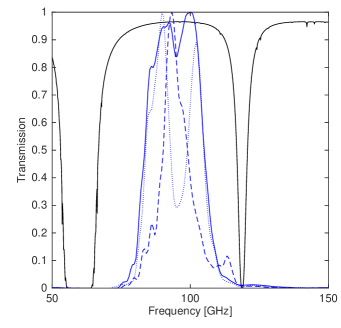
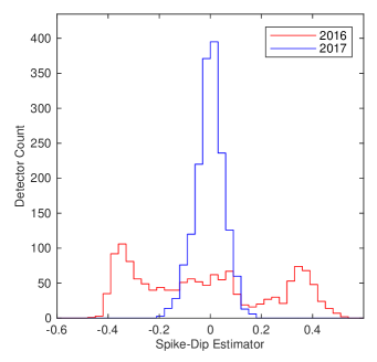
The delamination of the low-pass edge filters described in §3.6 resulted in non-uniform spectral features in the detectors during the 2016 season (Fig. 15) as well as a decrease in optical efficiency. We broadly observed two types of spectral variations: one where the response was suppressed at the outer edges of the nominal band which created a “spike” shaped profile, and one where the response was suppressed at the center of the band and created a “dip”. To further characterize this feature, we define an estimator $e$ :

\displaystyle e

\displaystyle=

\displaystyle\operatorname*{mean}_{\begin{subarray}{c}84<\nu<90\text{GHz}\\ 98<\nu<106\text{GHz}\end{subarray}}\left[B^{\prime}(\nu)\right]-\operatorname*{mean}_{\begin{subarray}{c}90<\nu<98\text{GHz}\end{subarray}}\left[B^{\prime}(\nu)\right]

(4)

where $B^{\prime}(\nu)=G(\nu;\sigma)*B(\nu)$ . $B(\nu)$ is the peak-normalized detector spectral response from FTS measurements, $G(\nu;\sigma)$ is a Gaussian with $\sigma=1$ GHz, and $B^{\prime}(\nu)$ is the detector spectrum convolved with the Gaussian smoothing kernel. The estimator $e$ takes on values $-1\leq e\leq 1$ , with $e<0$ being spike-like and $e>0$ being dip-like. The distribution of estimator values is shown in Fig. 16. All the low-pass edge filters were replaced at the end of the 2016 season, and no evidence of delamination has been found since their replacement. In order to determine the impact of these spectral features on the 2016 CMB data, we developed an additional jackknife test discussed further in §10.3.

High-frequency blue leaks originating from direct-island coupling to the TES bolometer are measured using a chopped liquid nitrogen source and a stack of thick grill high-pass filters (Timusk & Richards, 1981). These filters are machined metal plates with hex-packed circular holes corresponding to waveguide cutoff frequencies at 120, 170 and 247 GHz. Measurements showed response to a Raleigh-Jeans source of approximately 0.76 %, 0.61 % and 0.55 % above the 120 GHz, 170 GHz and 247 GHz edge, respectively.

8.2 Optical efficiency

We measured changes in optical power through detector load curves, by applying a high detector bias voltage to first drive the detector normal, then stepping down the bias voltage until the detector is superconducting. From these load curves, we can measure changes in optical power, assuming the total optical and electrical power is constant. The power difference is compared against the expected optical loading from an aperture-filling source at a known temperature, giving the end-to-end optical efficiency of the full system.

The change in optical loading is obtained by taking load curves while observing a source at ambient temperature ( $\sim 266$ K) and a liquid nitrogen (LN2) source at 74.2 K (at South Pole atmospheric pressure). For an aperture-filling, Rayleigh-Jeans source, the optical power $Q_{opt}$ deposited on a single-moded polarization-sensitive detector is

Q_{opt}=\frac{\eta}{2}\int\lambda^{2}S\left(\nu\right)B\left(\nu,T\right)d\nu

(5)

where $\eta$ is the optical efficiency, $B\left(\nu\right)$ is the Planck blackbody spectrum at temperature $T$ , and $S\left(\nu\right)$ is the detector spectral response. In the Rayleigh-Jeans limit ( $h\nu\ll kT$ ), Eq. 5 simplifies to

Q_{opt}=kT\eta\int S\left(\nu\right)d\nu=kT\eta\Delta\nu

(6)

where $\Delta\nu$ is the bandwidth and $\eta$ is the optical efficiency of the system. Observations of the sky and an aluminum mirror redirecting light into the cryostat provide estimates of the atmosphere and the internal cryostat photon load.

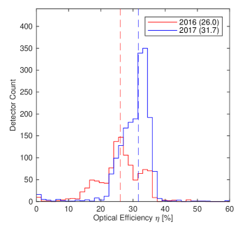
The Bicep3 per-detector optical efficiencies as measured using this method are shown in Fig. 17. The median end-to-end optical efficiency improved from $26\%$ in the 2016 season to $32\%$ in 2017. This is mostly due to the change in 300 K thermal filters described in §3.3 and the replacement of the delaminated metal-mesh edge filters described in §3.6.

8.3 Measured detector properties

We designed the thermal conductance of the detector to avoid saturation during science observations while minimizing phonon noise. The design saturation power of the Bicep3 detectors is 5 pW, which has a safety factor of 2-2.5 from the expected optical load during nominal observing conditions, giving a target thermal conductance $G_{c}=40$ pW/K for the titanium TES bolometer with transition temperature $T_{c}=500$ mK and a bath temperatures $T_{o}=280$ mK, where we assume a thermal index $\beta\sim 2$ from bare silicon nitride supports.

The detectors are screened prior to deployment to ensure that the properties are near target values. The thermal conductance $G_{c}$ , thermal conductance index $\beta$ , and transition temperature $T_{c}$ are given by

\displaystyle P_{\text{sat}}=G_{c}T_{o}\frac{\left(T_{c}/T_{o}\right)^{\beta+1}-1}{\beta+1}

(7)

where $P_{\text{sat}}$ is the saturation power of the detector. These parameters, shown in Table 7, are measured by taking load curves at multiple bath temperature $T_{o}$ in a “dark” configuration, where the cryostat is optically sealed to prevent light coupling to the detectors.

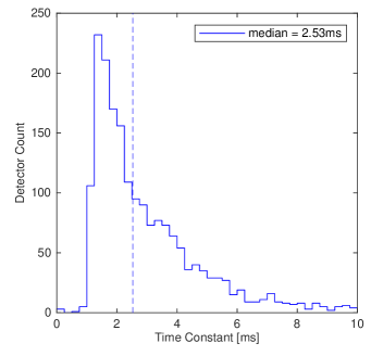
The effective thermal time constant $\tau$ of an ideal voltage-biased TES bolometer is given by

\displaystyle\tau=\frac{C/G}{1+\mathscr{L}\left(V\right)}

(8)

where $C$ is the heat capacity of the bolometer island and $\mathscr{L}$ is the effective loop gain of the electrothermal feedback at detector bias voltage $V$ . The detector time constants $\tau$ in Bicep3 are calculated by measuring the detector response to square-wave modulations in the bias voltage (Fig. 18).

Table 7: Average detector parameters for each Bicep3 module. Four of the modules, listed in parentheses, were replaced before the 2017 season. The normal resistance, saturation power, thermal conductance and transistion temperature are measured in a dark TES configuration before deployment for this subset of modules. The optical efficiency and spectral response were measured in situ at the South Pole. Fig. 9 shows the placement of the detector modules over the focal plane.

Module	Norm. Rest.	$\text{P}_{\text{sat}}@300$ mK	Thermal Conductance	Tran. Temp.	Band Center	Band Width
(P02)	81 m $\Omega$	3.71 pW	27.2 pW/K	503 mK	91 GHz	19 GHz
(P03)	83 m $\Omega$	3.01 pW	39.1 pW/K	514 mK	94 GHz	22 GHz
P04	92 m $\Omega$	4.76 pW	41.2 pW/K	492 mK	94 GHz	23 GHz
P06	65 m $\Omega$	4.25 pW	32.5 pW/K	501 mK	93 GHz	24 GHz
P07	61 m $\Omega$	4.56 pW	32.1 pW/K	507 mK	95 GHz	25 GHz
P08	63 m $\Omega$	4.33 pW	32.2 pW/K	505 mK	92 GHz	22 GHz
P09	63 m $\Omega$	5.61 pW	46.5 pW/K	479 mK	93 GHz	23 GHz
P10	49 m $\Omega$	5.03 pW	35.4 pW/K	513 mK	93 GHz	24 GHz
(P11)	138 m $\Omega$	6.72 pW	72.4 pW/K	478 mK	92 GHz	21 GHz
P12	78 m $\Omega$	5.57 pW	41.1 pW/K	494 mK	92 GHz	22 GHz
P13	78 m $\Omega$	5.97 pW	46.1 pW/K	487 mK	93 GHz	26 GHz
(P14)	153 m $\Omega$	–	–	–	92 GHz	22 GHz
P16	91 m $\Omega$	4.71 pW	31.6 pW/K	474 mK	95 GHz	18 GHz
P17	105 m $\Omega$	4.22 pW	56.2 pW/K	452 mK	93 GHz	20 GHz
P18	86 m $\Omega$	4.41 pW	36.4 pW/K	458 mK	95 GHz	23 GHz
P19	73 m $\Omega$	4.03 pW	31.3 pW/K	438 mK	93 GHz	24 GHz
P20	79 m $\Omega$	4.41 pW	32.4 pW/K	460 mK	93 GHz	22 GHz
P21	74 m $\Omega$	4.16 pW	32.3 pW/K	474 mK	95 GHz	26 GHz
P22	72 m $\Omega$	5.71 pW	46.4 pW/K	485 mK	93 GHz	21 GHz
P23	70 m $\Omega$	5.14 pW	42.3 pW/K	484 mK	93 GHz	24 GHz
P24	59 m $\Omega$	3.05 pW	26.4 pW/K	483 mK	93 GHz	24 GHz
P25	64 m $\Omega$	4.20 pW	32.7 pW/K	461 mK	93 GHz	24 GHz
P26	49 m $\Omega$	3.34 pW	24.9 pW/K	479 mK	93 GHz	24 GHz
P27	62 m $\Omega$	3.14 pW	27.2 pW/K	474 mK	93 GHz	24 GHz

8.4 Detector bias

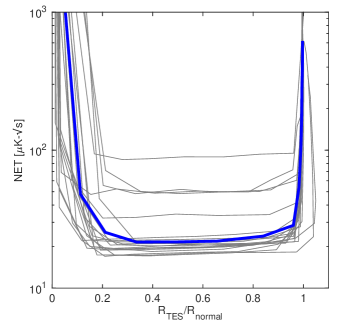
The detectors operate in strong electrothermal feedback to linearize the response and to speed up the time constant. The usable bias range is limited by thermal instability at low bias, and detector saturation at high bias as shown in Fig. 19. We believe thermal instability arises from finite thermal conductivity internal to the island which becomes problematic at the higher backgrounds at higher observing frequencies (Sonka et al., 2017).

The sensitivity of the detectors as a function of bias voltage is measured before each observing season to select the optimal bias. This is done by taking three-minute “noise stares” with the telescope at the nominal elevation for CMB observation, and comparing the noise levels obtained with the optical response as inferred from elevation nods (described in further detail in §9.3). Due to the multiplexing design, all detectors in one readout column share a common bias voltage. This limitation only modestly reduces system sensitivity as the per-detector NET is sufficiently insensitive to bias to allow a wide range of operating bias points.

8.5 Crosstalk

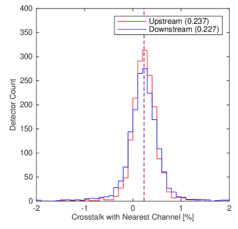
Crosstalk can occur between neighboring detectors within a readout column in the TDM system. One way to quantify the level of crosstalk through the readout chain is using cosmic rays. When a cosmic ray hits a detector, it generates a transient signal which may also trigger a faint signal in neighboring detectors in a readout column. We set up a custom analysis which searches unfiltered data to locate spikes from cosmic rays, stacks multiple events to increase the S/N, and compares the response in neighboring channels. Through this analysis, we find the crosstalk level in Bicep3 is consistent with previous experiments at $\sim 0.3\%$ . The fact that upstream is very similar to downstream crosstalk (see Fig. 20) argues that inductive crosstalk dominates over crosstalk from settling time crosstalk. The CMB temperature-to-polarization leakage due to crosstalk is quantified in the beam simulations shown in Appendix F of BICEP/Keck et al. (2021a).

8.6 Timestream noise

While the science audio band in Bicep3 is $\sim$ 0.1-1 Hz, the TDM readout system can alias higher frequency noise at multiples of the multiplexer’s Nyquist frequency into the science band. So we must model this high frequency noise, particularly in our readout electronics, and check that aliased noise does not compete with photon and phonon noise.

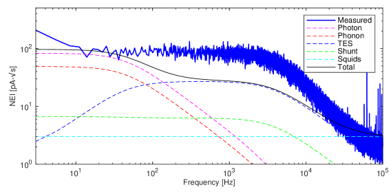
Fig. 21 shows the noise spectrum of a single detector under nominal observing conditions, as well as a model of the component contribution. The photon noise is

\displaystyle\mathrm{NEP}^{2}_{\text{photon}}

\displaystyle=2h\nu Q_{\mathrm{load}}+\frac{2Q^{2}_{\mathrm{load}}}{\nu\frac{\Delta\nu}{\nu}},

(9)

where $\nu$ is the frequency, $\frac{\Delta\nu}{\nu}$ is the fractional bandwidth, and $Q_{load}$ is the sum of astrophysical, atmospheric, and internal cryostat power loading. Table 4 summarizes all optical sources that contribute to $Q_{load}$ , dominated by the atmosphere. The computed photon noise dominates over the other internal noise mechanisms in the detector and electronics (Irwin & Hilton, 2005). The next most significant noise contribution comes from phonon noise,

\displaystyle\mathrm{NEP}^{2}_{\mathrm{phonon}}

\displaystyle=4kT^{2}_{c}G_{c}F\left(T_{c},T_{\mathrm{bath}}\right),

(10)

where $G_{c}$ is the thermal conductance, and $F(T_{c},T_{\mathrm{bath}})$ accounts for the distributed thermal conductance and is estimated to be $\sim 0.5$ . The Johnson noise, suppressed by the TES thermal feedback loop gain $\mathscr{L}$ , and the SQUID amplifier noise are subdominant at low frequencies.

As seen in Fig. 21, the measured total noise exceeds the calculated total at frequencies $\geq 100$ Hz. This excess noise lies above that predicted by simple noise models, and tends to be proportional to the slope of the superconducting transitions as described in Gildemeister et al. (2001). However, by setting the multiplexing rate to 25 kHz, we minimize aliasing most of this excess noise into the science audio band, leading to only a small contribution to the overall sensitivity (discussed in 10.4). Fortunately, Bicep3’s parameter choices with relatively low $G$ and relatively high multiplexing rate avoid the level of aliased excess noise observed in comparable experiments (Ade et al., 2015).

8.7 Near-field Beam Mapping

We measured the near-field angular response above the Bicep3 window during the austral summer at the South Pole in 2016 and 2017. These maps were obtained 53.5 cm above the primary lens (pupil), which represent a truncated map of the antenna response of each focal plane detector in its far field. These maps allow us to probe for various pathologies endemic to both the focal plane and optical elements before an extensive mapping campaign of the telescope far-field beams. The near-field beam maps are measured by observing a chopped $\sim 500$ K thermal source that is mounted on linear translation stages which allow for X/Y motion just above the aperture plane. The mapping apparatus is mounted directly onto the window such that the hot source is placed as close to the aperture stop as possible without incurring damage to the polyethylene vacuum window. The source is scanned across the plane of the aperture in a $50\times 50$ grid. At each step in this grid, the source remains stationary for $\sim 10$ seconds before proceeding to the next step.

Some Bicep2 and early Keck detectors demonstrated off-center near-field beam centers with a large truncation at the aperture stop, which both introduced distortions in the far-field beams and reduced the optical efficiency (Wong, 2014). This effect was traced to niobium contamination from the liftoff process during detector fabrication that introduced a phase shift across the planar antennas. Changing the fabrication to an “etch-back” process drastically reduced beam steer in Keck focal planes thereafter, and the same etching process was used in fabrication of Bicep3 modules (Buder et al., 2014). Fig. 22 shows beam steer measured across all detectors of Bicep3 compared to all detectors of the 95 GHz focal planes on Keck (both using the new etching process) and to Keck 150 GHz detectors (using the old process). While some beam steer still exists, the improved fabrication method led to a significant reduction in beam truncation at the aperture stop.

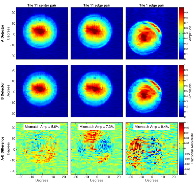
These measurements also characterize the mismatch in near-field beam centers between detectors within a given pair, which can arise either from a preferential steering of one detector in a pair, or from interactions between a detector at the tile edge and the surrounding corrugated frame (see §5.3). As shown in Fig. 23, a detectable increase in mismatch can be seen in detectors close to the corrugation frame which is at a level consistent with the simulations shown in Fig. 13. Combining this near-field beam map dataset with metrics derived from the far-field beam maps described in §8.8, we found no significant correlation between near-field beam steer and far-field beam shape in detectors which contribute to the final CMB data set.

8.8 Far-field Beam Mapping

Prior to the start of each observing season, Bicep3 undergoes an extensive far-field beam mapping (FFBM) campaign to characterize the shape of each beam in the telescope far-field. The compact aperture allows measurement of the far field ( $\sim$ 170 m for Bicep3) by placing a chopped source on a nearby ground-base location, the adjacent Martin A. Pomerantz Observatory (MAPO) building (where Keck was, and Bicep Array is, stationed), 200 m away from Bicep3. A 1.7 $\times$ 2.5 m flat aluminum mirror is erected at a 45^∘ angle above Bicep3, allowing the telescope to observe the source that is otherwise obstructed by the ground shield. The source is mounted on a 40 ft vertical mast above MAPO, consisting of a 24 inch aperture that is chopped between ambient blackbody ( $\sim 250$ K) and the sky at zenith ( $\sim 10$ K). Details of the setup and results of the pre-2016 season measurement are found in Karkare et al. (2016).

The raw beam map timestreams are demodulated at the chop rate to isolate the signal from the chopped source, and are binned into component maps with 0.1^∘ square pixels. Each beam is then fit to a 2D elliptical Gaussian:

B(\mathbf{x})=\frac{1}{\mathrm{A}}e^{-\frac{1}{2}(\mathbf{x}-\mathbf{\mu})^{T}\Sigma^{-1}(\mathbf{x}-\mathbf{\mu})}

(11)

where $\mathbf{x}$ is the two-dimensional coordinate of the beam center, $\mathbf{\mu}$ is the origin, $\mathrm{A}$ is the normalization, and $\Sigma$ is the covariance matrix, defined as

\displaystyle\Sigma=\quad\begin{pmatrix}\sigma^{2}(1+p)&c\sigma^{2}\\ c\sigma^{2}&\sigma^{2}(1-p)\end{pmatrix}

(12)

where $\sigma$ is the beamwidth, and $p$ and $c$ are plus and cross ellipticy, respectively. The fit values for Bicep3 are shown in Table 8 where the individual measurement uncertainty is the spread in parameter values over all component maps for a given detector, and is generally smaller than the detector-to-detector scatter. The median Gaussian beamwidth for Bicep3 is 0.161^∘, equivalent to a FWHM of 0.379^∘.

Table 8: Bicep3 median far-field beam parameters. These values are taken from 2017 FFBM data, and are presented as median over all detectors

\pm

scatter over all detectors

\pm

individual measurement uncertainty.

Parameter	Median $\pm$ Scatter $\pm$ Unc.
Beamwidth $\sigma$ (degrees)	$0.161\pm 0.003\pm 0.001$
Ellipticity plus $p$	$0.008\pm 0.002\pm 0.002$
Ellipticity cross $c$	$-0.010\pm 0.020\pm 0.019$
Diff. beamwidth $d\sigma$ (degrees)	$0.000\pm 0.001\pm 0.001$
Diff. ellipticity plus $dp$	$-0.003\pm 0.011\pm 0.002$
Diff. ellipticity cross $dc$	$-0.003\pm 0.004\pm 0.002$
Diff. pointing $dx$ (arcmin)	$-0.060\pm 0.120\pm 0.050$
Diff. pointing $dy$ (arcmin)	$0.000\pm 0.130\pm 0.050$

The component beam maps for each detector are then averaged together to create high-fidelity, per-detector composite beam maps. These composite beam maps are then coadded over all detectors to form the receiver-averaged beam, shown in Fig. 24. The receiver-averaged beams are then Fourier transformed and azimuthally averaged into the beam window function $B(\ell)$ which is inverted to recover the sky power spectrum. The per-detector composite beams are also used to quantify the temperature-to-polarization leakage in a given data set, which is done in Appendix F of BICEP/Keck et al. (2021a).

8.9 Polarization Response

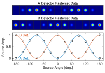
Unlike previous generations of Bicep receivers, Bicep3 did not use an aperture-filling rotating polarized source as shown in Takahashi et al. (2010). Instead the polarization response is acquired through observations of a rotating polarized quasi-thermal noise source (RPS). The source is placed on the same mast used in far-field beam measurements and observed via the large flat mirror described in §8.8. For a single observation, maps are created by rastering across the RPS in azimuth and stepping in elevation while keeping the polarization axis of the RPS at a fixed angle. 13 beam maps are created for RPS angles spanning $360^{\circ}$ in $30^{\circ}$ increments. Fig. 25 shows the resulting modulation in amplitude of the beams as a function of source polarization angle that produces a sinusoidal curve from which we derive detector polarization properties. The details and results from the RPS observations used here are described in Cornelison et al. (2020).

The relative polarization angles between detector pairs are measured to a precision of $<0.04^{\circ}$ , with a measured variation among pairs within each tile of $0.13^{\circ}$ rms, and variation of the median angles across tiles of $0.32^{\circ}$ rms. The small size of these variations allows us to use ideal, rather than measured per-detector polarization angles when creating Bicep3’s CMB polarization maps. Global polarization rotation is not as well constrained due to systematics arising in the geometry of the calibration itself. Instead, we estimate and subtract the global rotation angle from an EB/TB-minimization procedure to mitigate false B-mode signals (Kaufman et al., 2014).

The relative calibration of the polarization maps to the CMB temperature map shown in §9.3 depends on the level of cross-polar response of each detector, which is dominated by the crosstalk between the two detectors within a pair. The median cross-polar response is measured to be $0.7\pm 0.2\%$ , consistent with the crosstalk within the measurement uncertainty. While any difference between the measured and assumed cross-polar response contributes to additional uncertainty on the absolute gain calibration of the $E$ - and $B$ -mode polarization maps, it does not introduce any additional bias in the $B$ -mode signal.

8.10 Far-sidelobe Mapping

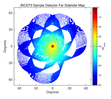
All Bicep/Keck receivers use two levels of warm baffling, to ensure that any ray must diffract twice to couple to the ground as described in §2.3. Any excess power in the far-sidelobe (FSL; roughly defined as the part of the beam outside the region captured by the co-moving forebaffle) should be coupled to an ambient-temperature absorber or redirected via the ground shield to cold sky. However, this power still increases the loading of the detectors, and if polarized, could lead to leakage that may be difficult to constrain. We therefore take measurements using a high-powered noise source to map the far-sidelobe region response. This measurement used the same noise source described in §8.9, which has variable attenuation that gives $\sim$ 70dB of dynamic range needed to map out all regions of the beam. The source is mounted on a mast on the same building as the Bicep3 instrument.

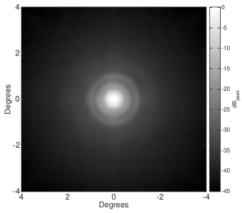
A typical far-sidelobe schedule takes 380^∘ scans in azimuth, with an elevation range of 34^∘ in 0.5^∘ steps, all repeated over multiple boresight rotation angles. The measurement is often repeated with both the co-moving forebaffle on and off, as an external check of the amount of power intercepting the forebaffle. A waveguide twist can be placed before the source output horn that couples to free space, in order to take measurements in two orthogonal source polarizations. Three different power settings are used to map out the entire beam at each boresight rotation angle, where the power settings are changed by adjusting the attenuation in the source. A “low” power setting maps the main beam, “medium” maps the mid-sidelobe, and “high” maps the far-sidelobe. The maps made with each setting are stitched together to create a single map for each detector. The maps at each polarization (made with and without the waveguide twist installed) can be coadded together to create an effective unpolarized FSL map. An example of this for a single Bicep3 detector is shown in Fig. 26.

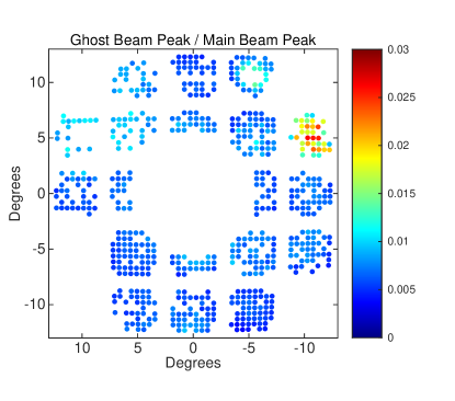
The FSL maps also reveal a small-amplitude, well-formed “ghost beam” located on the opposite side of the boresight from each detector’s main beam. In the time-reverse sense, the beam partially reflects off one of the flat 50 K filters and travels back through the 4 K optics, refocuses and reflects again off the focal plane to the emerging on sky. This feature has been seen in previous Bicep/Keck receivers (Bicep2 Collaboration et al., 2015) and for most detectors, the integrated power of this ghost beam is $<1$ % of the integrated main beam power. However, tile 1 shows integrated ghost beam power that is $2-3\times$ larger than that of the other detectors (Fig. 27). This anomalous ghost beam power is likely due to the non-symmetrical focal plane layout (Fig. 9). Bicep3 is equipped with 20 detector modules — slot 21, which is directly opposite to tile 1 on the focal plane, has no module and is covered by a reflective copper plate. Data from all detectors in tile 1 were thus removed from the final analysis in order to pass internal consistency checks.

9 Observing strategy

9.1 Observing field

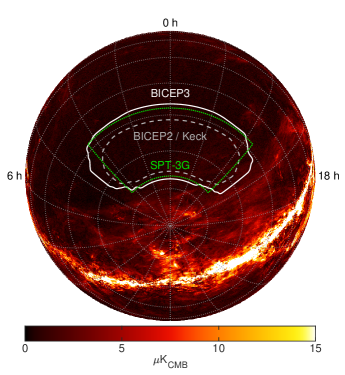
Bicep3 observes the same sky patch as Bicep2/Keck, covering $-60^{\circ}<\text{RA}<60^{\circ}$ and $-70^{\circ}<\delta<-40^{\circ}$ . However, its effective sky area is $\sim 600~{}\text{deg}^{2}$ , larger than the $\sim 400~{}\text{deg}^{2}$ in Bicep2/Keck due to the larger instantaneous field of view of Bicep3. To avoid regions of high dust contamination in this extended field, we slightly shifted the field center to $\text{RA}=0\text{hr}$ , $\text{dec}=-55^{\circ}$ , compared to $\text{RA}=0\text{hr}$ , $\text{dec}=-57.5^{\circ}$ for Bicep2/Keck. About 10% of the observing time is used to map a part of the Galactic plane, centered at $\text{RA}=15:42\text{hr}$ , $\text{dec}=-53^{\circ}$ .

This observing field is known to have very low polarized foregrounds, and is covered by other experiments (Fig. 28), providing the possibility for joint analyses. For example, we demonstrated in BICEP/Keck and SPTpol Collaboration et al. (2021) a method for separating the lensing $B$ -mode signal from the potential PGW signature in collaboration with SPT.

9.2 Scan pattern and schedule

Bicep3 observes its target CMB sky patch continuously through the austral winter season. At the South Pole, the telescope azimuth and elevation axes conveniently map to Right Ascension (RA) and Declination in equatorial coordinates, respectively. The sky patch then rotates in azimuth but does not move in elevation, allowing us to track it continuously.

The fundamental observing block is a constant-elevation ‘scanset’, consisting of 50 back-and-forth scans in azimuth, at $2.8^{\circ}$ /s spanning $64.4^{\circ}$ over 50 mins. Because the sky drifts by $12.5^{\circ}$ during each scanset, the azimuth center is shifted every other scanset by $25^{\circ}$ to track the change in RA of the target sky patch (Fig. 29). This azimuth-fixed scan pattern allows us to remove ground-fixed pickup and terrestrial magnetic contamination with a simple ground-subtraction template. The elevation is stepped every other scanset by $0.25^{\circ}$ to fill in coverage between the spatially separated detector beams.

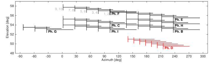
The overall schedule contains cryogenic service and CMB and Galactic plane scansets. These scansets are grouped into ‘observing phases’, and each phase contains between 6 to 10 scansets along with the accompanying calibrations. During a three-day schedule, the telescope completes one cryogenic cycle, six 10-hour phases on the CMB field, one 6-hr phase on the CMB field, and one 6-hr phase on the Galactic plane (Table 9).

The telescope is rotated about its optical axis to a different boresight angle for each schedule. A total of four boresight angles at $23^{\circ}$ , $68^{\circ}$ , $203^{\circ}$ and $268^{\circ}$ are used. The $45^{\circ}$ pairs are required to measure both the Stokes $Q$ and $U$ parameters. The whole set of four angles is clocked to optimize the coverage symmetry and homogeneity over the target CMB sky patch.

Table 9: Observation schedule for Bicep3. Start times are listed by Local Sidereal Time (LST). The 2016 season used a two-day schedule without the bolded phases G, H and I.

Phase	LST	Field	No. of Scansets
A	Day 0 23:00	Fridge re-cycling
B	Day 1 05:00	CMB	10
C	Day 1 14:00	CMB	10
D	Day 1 23:00	Galactic	7
E	Day 2 05:00	CMB	10
F	Day 2 14:00	CMB	10
G	Day 2 23:00	CMB	6
H	Day 3 05:00	CMB	10
I	Day 3 14:00	CMB	10

9.3 Detector calibrations

The detectors in Bicep3 are calibrated in two steps. First, a relative gain calibration is applied to ensure the timestream data from each detector pair accurately subtracts the large common-mode unpolarized signals from the atmosphere, telescope and CMB. Each scanset is bracketed by an elevation nod (elnod) where the telescope is stepped upward by 0.6^∘ then downward by 1.2^∘, and finally upward again by 0.6^∘ to return to the starting position over the course of one minute. This motion causes all of the detectors to measure varying levels of atmospheric emission according to the relative opacity $\kappa$ of the atmosphere is described by

\displaystyle\kappa

\displaystyle=

\displaystyle\frac{1}{\sin\left(\text{el}\right)}

(13)

down to elevation el $=30^{\circ}$ . Each leading and trailing elnod gives a mean gain of detector native feedback units (FBU) per airmass for each channel for the scanset, allowing us to relatively calibrate all the detectors. A larger ‘sky dip’ spanning 50^∘ to 90^∘ is performed before each phase as an additional calibration data point for confirming the atmospheric profile.

In addition to the relative gain calibration, the final data set requires an absolute gain calibration. We apply a single scale factor to convert from detector FBU to final CMB temperature units. This scale factor $g_{\text{abs}}$ is determined by computing the ratio of the cross spectra of the Bicep3 map with external, calibrated maps from Planck. We first calculate

g_{b}=\frac{\left<\tilde{m}_{\text{cal}}\times\tilde{m}_{\text{ref}}\right>_{b}}{\left<\tilde{m}_{\text{real}}\times\tilde{m}_{\text{ref}}\right>_{b}},

(14)

where $\tilde{m}_{\text{real}}$ is the uncalibrated Bicep3 temperature map, and $\tilde{m}_{\text{cal}}$ and $\tilde{m}_{\text{ref}}$ are the Planck 95 and 145 GHz maps respectively. Two separate external maps are used to reduce noise. The Planck maps are smoothed by Bicep3’s beam and reobserved using the same filtering applied to the Bicep3 maps. The ratio of these two spectra is a set of bandpower calibration factors $g_{b}$ . The final scale factor $g_{\text{abs}}$ uses the mean of the first five bandpowers $g_{b}$ of the Bicep/Keck bins.

9.4 Star pointing

‘Star pointing’ optical pointing measurements are made with the star camera every few weeks. It has become a routine observation to track the small movements of the telescope mount built on top of snow, though the frequency and quality of star pointings varies depending on the weather. The goal of star pointing observations is to verify the parameters used in the telescope pointing model are stable, including three tilt and two zero-offset parameters along the azimuth and elevation directions, as well as two parameters associated with the offset of the star camera from the mount’s boresight rotation axis.

Two separate lists of stars for summer (12 stars) and winter (29 stars) accommodate the change in visibility. The entire set of stars is observed at three distinct deck angles, yielding three sets of independent data points. The sequence involves centering each star, in turn, on the star camera’s boresight crosshairs (in practice, one predefined pixel in the CCD), and recording the mount encoders and the current time. This is done for each star at three different boresight rotation angles. The pointing model parameters can be found by fitting the telescope pointing against the star positions. In this process, outliers are dropped and only those schedules with more than 24 data points (in the winter) are kept for data fitting. The root mean square of the fit residuals typically reach $\sim 20$ arcsec.

During the analysis of the 2016 data, we noticed the temporal split jackknife (see discussion in §10.3) showed exceptionally low statistical probabilities. It was eventually traced to shift in the elevation offset parameter derived from star pointings. There was a clear $0.02^{\circ}$ shift in this parameter roughly halfway through the season, leading to the jackknife test failures. We associated this shift with a mechanical slip in the star camera mount that was not aligned with the boresight of the telescope, and we added a flexure term in the pointing model to capture this effect and correct the jackknife failures. In the subsequent investigation, we correlated per-schedule CMB maps against reobserved Planck CMB maps. This provided a high temporal resolution boresight tracker to monitor pointing shifts to sub arc-min levels, and corroborated our assumption about the pointing shift. This analysis has been incorporated to track anomalous changes in tilting and offset parameters in Bicep and Keck telescopes.

10 Three-year data set

10.1 Data selection and cuts

Bicep3 was installed in the Dark Sector Laboratory (DSL) at the South Pole on December of 2014 with a partially filled focal plane. It was populated with a full complement of 20 detector tiles in December of 2015 and began scientifically meaningful observations in early 2016. Grayson et al. (2016) and Hui et al. (2016) show preliminary data quality of Bicep3 during the 2016 season. After the 2016 season, the telescope was removed from the mount and modified during the austral summer. These modifications improved the detector yield, the observation efficiency, and the noise performance, ultimately improving the sensitivity by $\sim 30\%$ compared to the previous season (Kang et al., 2018).

The detector wafers in Bicep3 were fabricated at the JPL Microdevices Laboratory. 90% of the wafers achieved $\geq 82\%$ in room temperature impedance screening. The majority of the detector yield losses are associated with wirebond failures in the readout chain. There are more than 22,000 wirebonds in Bicep3, connecting between detector wafers, SQUIDs amplifier chips, and various circuit boards. Failures in critical wirebonds can disable an entire readout column of 22 detectors or an entire row of 30 detectors.

The fully-populated focal plane has 1200 optically active dual-polarized detector pairs. At optimal TES bias values, there were 930, 992, and 992 responsive detector pairs in 2016, 2017 and 2018, respectively. Detectors were further down-selected during analysis based on performance in CMB observations and various external calibration measurements. The achieved efficiency in CMB observations and the progression of map sensitivity are shown in Fig. 30. Data selection (‘cut’) parameters and statistics are shown in Table 10. The last round of data down-selection, so-called ‘channel flags’, excludes detectors that are found to be discrepant during map-making and external calibration measurements. These may include aberrant beams, absolute calibrations, and the exclusion of Tile 1 channel discussed in §8.10. These detectors are removed for the entire season, and their data are thus excluded from the final coadded maps. The rest of the cut parameters probe a wide variety of data quality metrics at per-detector pair, per-scanset, and per-halfscan levels. Out of all the responsive detector pairs, Bicep3 achieved overall pass fractions of 57.0%, 65.8%, and 61.8% in 2016, 2017 and 2018, respectively.

Table 10: Data Cuts as described in Appendix A of Willmert (2019). These cuts are applied sequentially, in the order listed. The first column (raw) shows the fraction of data removed by the cut parameter, if no other cuts were considered. For rows after the second, this value is referenced against the total fraction of data from nominally “functional” detectors. The second column shows the fractional remaining data after each sequentially applied round of cuts. Horizontal lines distinguish between (from top to bottom) focal plane yield, cuts applied per-halfscan, cuts applied per-scanset, cuts on cuts, and post-hoc per-pair ‘channel flag’ cuts determined at the mapmaking stage.

	2016 Cuts [%]		2017 Cuts [%]		2018 Cuts [%]
Cut Parameter	Raw	Remaining	Raw	Remaining	Raw	Remaining
Before cuts	-	100.0	-	100.0	-	100.0
Non-functional detectors	22.54	77.5	17.29	82.7	17.29	82.7
Timestream glitches/dropped samples	0.62	76.8	0.13	82.6	0.13	82.6
Intra-MCE synchronization	0.00	76.8	0.06	82.6	0.00	82.6
Inter-MCE synchronization	0.00	76.8	0.04	82.6	0.00	82.6
Frac. of passing channels (MUX col.)	0.10	76.8	0.08	82.6	0.02	82.6
Frac. of passing channels (full expt.)	0.00	76.8	0.07	82.6	0.02	82.6
Raw elnod amplitude not negligible	14.54	62.9	12.45	70.2	13.14	69.6
Elnod stability over scanset	11.56	60.9	9.80	68.7	11.59	66.8
Elnod A/B ratio stability over scanset	16.25	59.3	13.14	67.8	14.03	66.0
Glitches in elnod	2.72	57.8	1.36	66.9	1.55	65.0
Pair-sum elnod model goodness-of-fit	10.65	53.4	6.29	64.5	9.53	62.1
Pair-difference elnod shows structure	6.19	52.7	4.25	64.0	5.61	61.9
TES resistance	2.14	52.1	1.27	63.7	0.94	61.7
Median elnod amplitude	0.40	52.1	0.48	63.7	1.46	61.7
Pair-difference timestream skewness	9.23	51.3	6.54	63.3	8.85	60.4
Change in azimuth-fixed signal during scanset	2.28	51.2	1.91	63.2	2.08	60.4
Excessively high timestream STD	18.57	49.8	14.92	62.4	15.92	59.7
Focal plane-correlated noise	0.00	49.8	0.00	62.4	0.00	59.7
Noise stationarity (per-detector)	5.96	49.2	4.99	61.6	7.10	58.8
Noise stationarity (per-pair)	10.64	49.1	8.00	61.6	10.51	58.7
Mean focal plane temperature	0.00	49.1	0.00	61.6	0.00	58.7
Focal plane temperature stability	0.37	49.0	0.76	61.3	0.27	58.6
Abnormal azimuth scanning	0.02	49.0	0.00	61.3	0.00	58.6
Too many large steps in timestream	0.53	49.0	0.14	61.3	0.38	58.6
Too many de-stepping attempts	10.04	48.1	7.85	60.2	11.91	56.6
Extreme/variable crosstalk	0.23	47.9	0.16	60.1	0.38	56.3
Frac. of passing halfscans	1.22	47.9	0.49	60.1	1.35	56.3
Frac. of passing data in scanset	9.02	47.4	6.52	59.9	9.59	56.1
Per-pair mapmaking cuts (inc. drop tile 1)	-	44.2	-	54.4	-	51.1

10.2 Data reduction

The data reduction and map making pipeline used in Bicep3 is largely the same as the Bicep2/Keck procedure detailed in BICEP2 collaboration et al. (2014b), with only minor modifications to accommodate the larger number of detectors.

10.3 Jackknife Tests

As a standard internal consistency check, we split each year’s data set into two halves in various ways. These halves are differenced to cancel out the common signal and leave only noise and the potential contribution of systematic errors. Following previous experiments, we use 14 different jackknifes listed in Bicep2 Collaboration et al. (2015) to probe temporal, spatial and readout systematics.

For a given jackknife $j$ , a vector of bandpowers of $\mathbf{d}_{j}$ is compared to the bandpowers from the ensemble of 499 signal+noise simulations $\mathbf{s}_{j}$ by calculating $\chi$ and $\chi^{2}$ statistics, defined as:

	$\displaystyle\chi$	$\displaystyle=$	$\displaystyle\sum_{b}\frac{\left[\mathbf{d}_{j}\right]_{b}-\left<\mathbf{s}_{j}\right>_{b}}{\left[\mathbf{S}_{j}\right]_{bb}}$
	$\displaystyle\chi^{2}_{j}$	$\displaystyle=$	$\displaystyle\left(\mathbf{d}_{j}-\left<\mathbf{s}_{j}\right>\right)^{\top}\mathbf{S}_{j}^{-1}\left(\mathbf{d}_{j}-\left<\mathbf{s}_{j}\right>\right)$		(15)

where $\mathbf{S}_{j}=\left<\mathbf{s}_{j}\mathbf{s}_{j}^{\top}\right>$ is the bandpower covariance matrix of the corresponding simulations for a single spectral type. The $\chi$ and $\chi^{2}$ values are calculated for real data against the full ensemble, and the real data are judged against the distribution of statistics obtained from the simulations by computing the probability to exceed (PTE).

For the three-year data set, we performed jackknife tests on each year separately, giving a total of $3(\text{EE/BB/EB})\times 14(\text{jack})\times 2(\chi/\chi^{2})\times 2(\text{bin})\times 3(\text{year})=504$ tests. A statistical failure led to the discovery and removal of the tile 1 data discussed in §8.10, and the injection of a flexure term to the pointing model discussed in §9.4. All the jackknife tests were then repeated with the updated data set and the final PTE values from the $\chi$ and $\chi^{2}$ statistics are listed in Table 11. Fig. 31 shows the distributions of these PTE values, which appear to be uniform, showing no evidence of problems at the level of statistical noise.

Table 11: Jackknife PTE values from

\chi

and

\chi^{2}

tests.

	2016		2017		2018
	$\chi$	$\chi^{2}$	$\chi$	$\chi^{2}$	$\chi$	$\chi^{2}$
Band Power	1-5/1-9
Deck jackknife
EE	0.501/0.383	0.754/0.719	0.982/0.992	0.050/0.108	0.022/0.172	0.122/0.092
BB	0.936/0.998	0.443/0.226	0.731/0.419	0.848/0.563	0.567/0.924	0.130/0.152
EB	0.319/0.283	0.840/0.866	0.263/0.589	0.932/0.838	0.265/0.307	0.832/0.868
Scan dir jackknife
EE	0.277/0.112	0.956/0.275	0.449/0.453	0.066/0.070	0.198/0.437	0.804/0.459
BB	0.764/0.872	0.525/0.196	0.283/0.433	0.162/0.407	0.168/0.172	0.012/0.030
EB	0.904/0.431	0.697/0.591	0.076/0.228	0.517/0.816	0.838/0.527	0.806/0.798
Temporal split jackknife
EE	0.998/0.996	0.084/0.257	0.028/0.068	0.277/0.295	0.146/0.467	0.395/0.152
BB	0.098/0.200	0.261/0.255	0.263/0.531	0.331/0.317	0.826/0.946	0.822/0.719
EB	0.958/0.772	0.461/0.713	0.956/0.936	0.020/0.044	0.070/0.034	0.497/0.499
Tile jackknife
EE	0.257/0.150	0.429/0.623	0.403/0.529	0.559/0.248	0.002/0.004	0.004/0.018
BB	0.527/0.713	0.323/0.495	0.952/0.852	0.455/0.816	0.697/0.862	0.705/0.371
EB	0.707/0.493	0.776/0.872	0.381/0.633	0.517/0.311	0.946/0.984	0.146/0.257
Azimuth jackknife
EE	0.575/0.866	0.140/0.259	0.776/0.727	0.916/0.962	0.834/0.545	0.695/0.687
BB	0.014/0.126	0.082/0.068	0.178/0.425	0.435/0.667	0.487/0.279	0.860/0.665
EB	0.357/0.415	0.846/0.212	0.487/0.068	0.904/0.363	0.876/0.998	0.164/0.040
Mux col jackknife
EE	0.309/0.429	0.335/0.363	0.731/0.745	0.232/0.625	0.681/0.946	0.894/0.778
BB	0.665/0.182	0.960/0.423	0.116/0.070	0.840/0.950	0.210/0.657	0.573/0.108
EB	0.451/0.681	0.944/0.992	0.335/0.339	0.423/0.415	0.248/0.353	0.988/0.924
Alt deck jackknife
EE	0.982/0.996	0.220/0.166	0.972/0.954	0.172/0.405	0.056/0.182	0.102/0.214
BB	0.062/0.635	0.307/0.170	0.251/0.236	0.050/0.100	0.054/0.467	0.152/0.042
EB	0.198/0.192	0.477/0.790	0.411/0.731	0.238/0.118	0.667/0.429	0.513/0.814
Mux row jackknife
EE	0.776/0.796	0.144/0.068	0.914/0.824	0.345/0.447	0.741/0.359	0.707/0.719
BB	0.822/0.725	0.539/0.631	0.425/0.631	0.561/0.800	0.515/0.673	0.890/0.583
EB	0.850/0.471	0.060/0.166	0.677/0.573	0.383/0.677	0.367/0.601	0.870/0.844
Tile and deck jackknife
EE	0.631/0.421	0.788/0.878	0.439/0.427	0.888/0.920	0.886/0.926	0.715/0.902
BB	0.902/0.904	0.531/0.477	0.601/0.786	0.441/0.407	0.411/0.567	0.349/0.695
EB	0.311/0.461	0.429/0.569	0.842/0.709	0.204/0.377	0.896/0.944	0.733/0.485
Focal plane inner or outer jackknife
EE	0.355/0.635	0.822/0.311	0.204/0.224	0.579/0.633	0.174/0.120	0.208/0.327
BB	0.800/0.922	0.711/0.555	0.663/0.928	0.617/0.295	0.148/0.194	0.204/0.283
EB	0.483/0.760	0.303/0.373	0.836/0.974	0.711/0.549	0.132/0.130	0.880/0.635
Tile top or bottom jackknife
EE	0.942/0.641	0.064/0.010	0.768/0.960	0.505/0.397	0.910/0.679	0.204/0.463
BB	0.974/0.764	0.124/0.012	0.224/0.703	0.046/0.090	0.226/0.705	0.774/0.503
EB	0.353/0.717	0.675/0.593	0.786/0.932	0.411/0.451	0.136/0.345	0.148/0.174
Tile inner or outer jackknife
EE	0.745/0.665	0.397/0.798	0.828/0.870	0.756/0.930	0.002/0.012	0.014/0.124
BB	0.337/0.667	0.224/0.421	0.196/0.667	0.956/0.818	0.810/0.924	0.076/0.138
EB	0.820/0.900	0.840/0.922	0.216/0.405	0.583/0.756	0.321/0.545	0.321/0.635
Moon jackknife
EE	0.218/0.709	0.485/0.487	0.860/0.882	0.780/0.878	0.904/0.683	0.104/0.160
BB	0.976/0.824	0.255/0.607	0.996/0.946	0.108/0.246	0.206/0.164	0.142/0.385
EB	0.487/0.900	0.778/0.693	0.088/0.128	0.583/0.463	0.840/0.912	0.701/0.064
A and B offset best and worst jackknife
EE	0.860/0.794	0.723/0.924	0.571/0.661	0.315/0.537	0.860/0.625	0.908/0.565
BB	0.453/0.561	0.022/0.044	0.970/0.972	0.194/0.293	0.860/0.942	0.814/0.780
EB	0.435/0.455	0.259/0.549	0.806/0.760	0.421/0.285	0.806/0.623	0.776/0.551

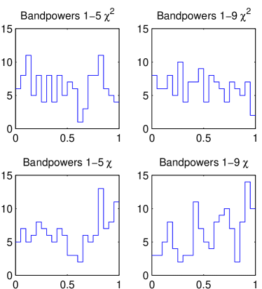
In addition to the standard 14 jackknife tests, we created an additional spectral jackknife to test the spectral anomaly in the 2016 data due to the metal mesh low-pass edge filter delamination described in §3.6. Using the definition in Eq. 4, we selected the worst 50% (the most spikes and dips) of the data, and compared it to the coadded 2017/18 data which has an uniform spectral response. With 99 simulations, we found the difference is consistent with a null result (Fig. 32).

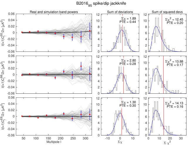
10.4 Instantaneous sensitivity

During normal CMB observation, the detector timestreams are multiplexed, downsampled and filtered to 30 Hz, which is sufficient for the 0.1-1 Hz science band. 1/ $f$ noise dominated by atmospheric noise, is greatly reduced after pairs of co-located polarization sensitive detectors are differenced. Contamination from the atmosphere and ground signals is further suppressed by filtering the timestreams with a third-order polynomial and subtracting a ground-averaged template from the scanning data (Fig. 33).

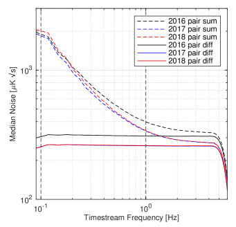
The per-detector, per-scanset noise distribution is shown in Fig. 34. The median pair-difference, per-detector sensitivity of 312 $\mu\mathrm{K}_{\mathrm{\mbox{\tiny\sc cmb}}}\sqrt{\mathrm{s}}$ and 263 $\mu\mathrm{K}_{\mathrm{\mbox{\tiny\sc cmb}}}\sqrt{\mathrm{s}}$ is achieved in 2016 and 2017/18 data, respectively. The sensitivity includes the weighted combination of every individual detector in every scanset during the three-year observation, capturing both the telescope performance and Antarctic seasonal variation.

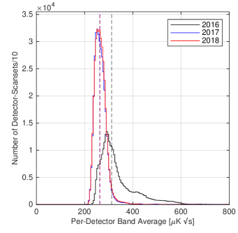
We estimate the noise performance of the full Bicep3 instrument by calculating the inverse variance weight used in the final maps, giving the average Bicep3 noise equivalent temperature (NET) as 9.15, 6.82 and 7.14 $\mu\mathrm{K}_{\mathrm{\mbox{\tiny\sc cmb}}}\sqrt{\mathrm{s}}$ in 2016, 2017 and 2018, respectively, after all cuts are applied.

10.5 Map depth

The map depth is a measure of the noise level in the polarization maps. Together with the area of the maps, the map depth $D$ , which we define as the deepest, central part of the map (BICEP2 collaboration et al., 2014b), sets the final statistical sensitivity of the experiment. This calculation accounts for the nonuniform coverage of the field, weighting each map pixel by its contribution relative to the deepest part of the map. The effective area $A_{\text{eff}}$ is calculated using the apodization mask to ensure the maps smoothly fall to zero, thus accounting for the higher variance and lower weight at the edges of the map. The total sensitivity, $T=D/\sqrt{A_{\text{eff}}}$ , gives a single number in temperature units indicating the total $B$ -mode statistical sensitivity.

Table 12 lists the performance for Bicep3. We achieved a map depth of 2.8 $\mu$ K-arcmin over an effective area of 584.9 $\text{deg}^{2}$ , for a total sensitivity of $T=1.3$ nK from the three-year Bicep3 data set. The final T, Q, U maps and their corresponding noise are shown in Fig. 35.

Table 12: Bicep3 map based sensitivity by season

Season	Map Depth ( $D$ )	Eff. Area ( $A_{\text{eff}}$ )	Total Sen. ( $T$ )
2016	5.9 $\mu\text{K-arcmin}$	569.2 $\text{deg}^{2}$	2.9 nK
2017	4.4 $\mu\text{K-arcmin}$	588.1 $\text{deg}^{2}$	2.2 nK
2018	4.4 $\mu\text{K-arcmin}$	584.7 $\text{deg}^{2}$	2.1 nK
Total	2.8 $\mu\text{K-arcmin}$	584.9 $\text{deg}^{2}$	1.3 nK

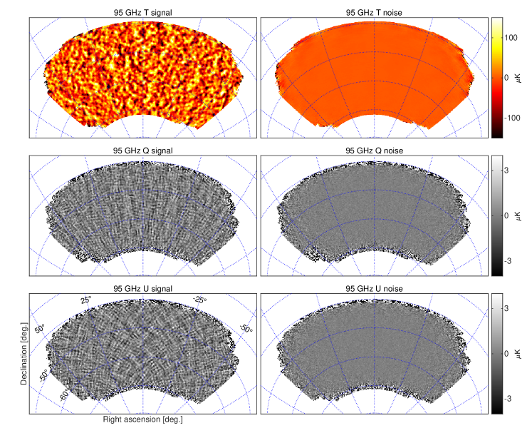
11 Conclusions

We presented the design and performance of Bicep3, which has been observing CMB polarization from the South Pole since 2016. The three-year data set, from 2016-2018, reached a map depth of 2.8 $\mu$ K-arcmin (46 nK-deg) over an effective area of 584.9 square degrees, corresponding to a total sensitivity of $T=1.3$ nK. A suite of jackknife tests show possible sources of systematic false polarization are controlled below the level of statistical sensitivity in each test.

In BICEP/Keck et al. (2021a) we present a cosmological analysis using this three-year Bicep3 data set with the combination of data from Keck. The combination improve the sensitivity on $r$ to $\sigma(r)=0.009$ . During the austral summers at 2018 and 2019, we observed the CMB cold spot anomaly, which is detailed in Kang et al. (2020). With its achieved sensitivity, Bicep3 can also be utilized for a number of additional science targets, including primordial magnetic fields and axion-like particles through anisotropic and time-variable cosmic birefringence (BICEP2 Collaboration et al., 2017; BICEP/Keck et al., 2021b), the properties of interstellar dust grains (Clark & Hensley, 2019), and patchy reionization and gravitational lensing through the use of distortion metrics (Yadav et al., 2010).

Additional Bicep3 data taken from 2019 to 2021 are expected to further reduce noise in the 95 GHz power spectrum by a factor greater than $\sqrt{2}$ . Bicep Array, which is based on the design of Bicep3, deployed the first of four receivers at 30/40 GHz to the South Pole in 2020. In coming years, additional receivers will be deployed at 95, 150 and 220/270 GHz with 32,000+ total detectors (Moncelsi et al., 2020). We project the Bicep/Keck experiment to reach $\sigma(r)$ between 0.002 and 0.004 at the end of Bicep Array, depending on foreground complexity and degree of removal of $B$ -modes due to gravitational lensing (BICEP/Keck and SPTpol Collaboration et al., 2021).

Bicep/Keck has been made possible through a series of grants from the National Science Foundation including 0742818, 0742592, 1044978, 1110087, 1145172, 1145143, 1145248, 1639040, 1638957, 1638978, 1638970, 1836010 and by the Keck Foundation. The construction of the Bicep3 receiver was supported by the Department of Energy, Laboratory Directed Research and Development program at SLAC National Accelerator Laboratory, under contract DE-AC02-76SF00515. The development of antenna-coupled detector technology was supported by the JPL Research and Technology Development Fund and Grants No. 06-ARPA206-0040 and 10-SAT10-0017 from the NASA APRA and SAT programs. The development and testing of focal planes were supported by the Gordon and Betty Moore Foundation at Caltech. Readout electronics were supported by a Canada Foundation for Innovation grant to UBC. The computations in this paper were run on the Cannon cluster supported by the FAS Science Division Research Computing Group at Harvard University. We thank the staff of the U.S. Antarctic Program and in particular the South Pole Station without whose help this research would not have been possible. Most special thanks go to our heroic winter-overs Sam Harrison, Hans Boenish, Grantland Hall, Ta-Lee Shue, Paula Crock, and Calvin Tsai. We thank all those who have contributed past efforts to the Bicep/Keck series of experiments, including the Bicep1 team. We would also like to thank Jonathon Hunacek at JPL/Caltech for exchange of information regarding detector readout and laboratory housekeeping design, and Aritoki Suzuki, Oliver Jeong, Yuki Inoue, Tomotake Matsumura at Berkeley and in Japan for discussions regarding alumina optics and AR coatings.

References

Ade et al. (2008) Ade, P., Bock, J., Bowden, M., et al. 2008, Astrophys. J., 674, 22, doi: 10.1086/524922
Ade et al. (2006) Ade, P. A. R., Pisano, G., Tucker, C., & Weaver, S. 2006, in A review of metal mesh filters, Vol. 6275, 62750U–62750U–15
Ade et al. (2015) Ade, P. A. R., Aikin, R. W., Amiri, M., et al. 2015, The Astrophysical Journal, 812, 176
Ahmed et al. (2014) Ahmed, Z., Grayson, J. A., Thompson, K. L., et al. 2014, Journal of Low Temperature Physics, 176, 835
Albrecht & Steinhardt (1982) Albrecht, A., & Steinhardt, P. J. 1982, Phys. Rev. Lett., 48, 1220, doi: 10.1103/PhysRevLett.48.1220
Barkats et al. (2018) Barkats, D., Dierickx, M. I., Kovac, J. M., et al. 2018, in Society of Photo-Optical Instrumentation Engineers (SPIE) Conference Series, Vol. 10708, Millimeter, Submillimeter, and Far-Infrared Detectors and Instrumentation for Astronomy IX, ed. J. Zmuidzinas & J.-R. Gao, 107082K, doi: 10.1117/12.2312585
Battistelli et al. (2008) Battistelli, E. S., Amiri, M., Burger, B., et al. 2008, Journal of Low Temperature Physics, 151, 908
BICEP2 collaboration et al. (2014a) BICEP2 collaboration, Ade, P. A. R., Aikin, R. W., et al. 2014a, Phys. Rev. Lett., 112, 241101
BICEP2 collaboration et al. (2014b) —. 2014b, The Astrophysical Journal, 792, 62
Bicep2 Collaboration et al. (2015) Bicep2 Collaboration, Ade, P. A. R., Aikin, R. W., et al. 2015, Astrophys. J., 814, 110, doi: 10.1088/0004-637X/814/2/110
BICEP2 Collaboration et al. (2017) BICEP2 Collaboration, Keck Array Collaboration, Ade, P. A. R., et al. 2017, Phys. Rev. D, 96, 102003, doi: 10.1103/PhysRevD.96.102003
BICEP2/Keck and Planck collaborations et al. (2015) BICEP2/Keck and Planck collaborations, Ade, P. A. R., Aghanim, N., Ahmed, Z., et al. 2015, Phys. Rev. Lett., 114, 101301
BICEP/Keck et al. (2021a) BICEP/Keck, Ade, P. A. R., Ahmed, Z., et al. 2021a, Phys. Rev. D, 103, 042002, doi: 10.1103/PhysRevD.103.042002
BICEP/Keck et al. (2021b) —. 2021b, Phys. Rev. D, 103, 042002, doi: 10.1103/PhysRevD.103.042002
BICEP/Keck and SPTpol Collaboration et al. (2021) BICEP/Keck and SPTpol Collaboration, Ade, P. A. R., Ahmed, Z., et al. 2021, Phys. Rev. D, 103, 022004, doi: 10.1103/PhysRevD.103.022004
Brout et al. (1978) Brout, R., Englert, F., & Gunzig, E. 1978, Annals of Physics, 115, 78, doi: 10.1016/0003-4916(78)90176-8
Buder et al. (2014) Buder, I., Ade, P. A. R., Ahmed, Z., et al. 2014, in Society of Photo-Optical Instrumentation Engineers (SPIE) Conference Series, Vol. 9153, Millimeter, Submillimeter, and Far-Infrared Detectors and Instrumentation for Astronomy VII, ed. W. S. Holland & J. Zmuidzinas, 915312, doi: 10.1117/12.2055713
Chiang et al. (2010) Chiang, H. C., Ade, P. A. R., Barkats, D., et al. 2010, Astrophys. J., 711, 1123, doi: 10.1088/0004-637X/711/2/1123
Clark & Hensley (2019) Clark, S. E., & Hensley, B. S. 2019, Astrophys. J., 887, 136, doi: 10.3847/1538-4357/ab5803
Cornelison et al. (2020) Cornelison, J., Ade, P. A. R., Ahmed, Z., et al. 2020, in Millimeter, Submillimeter, and Far-Infrared Detectors and Instrumentation for Astronomy X, ed. J. Zmuidzinas & J.-R. Gao, Vol. 11453, International Society for Optics and Photonics (SPIE), 302 – 313, doi: 10.1117/12.2562905
Crumrine et al. (2018) Crumrine, M., Ade, P. A. R., Ahmed, Z., et al. 2018, in Society of Photo-Optical Instrumentation Engineers (SPIE) Conference Series, Vol. 10708, Millimeter, Submillimeter, and Far-Infrared Detectors and Instrumentation for Astronomy IX, ed. J. Zmuidzinas & J.-R. Gao, 107082D, doi: 10.1117/12.2312829
Cukierman et al. (2020) Cukierman, A., Ahmed, Z., Henderson, S., et al. 2020, Journal of Low Temperature Physics, 199, 858, doi: 10.1007/s10909-019-02296-2
Dahal et al. (2020) Dahal, S., Amiri, M., Appel, J. W., et al. 2020, Journal of Low Temperature Physics, 199, 289, doi: 10.1007/s10909-019-02317-0
de Korte et al. (2003) de Korte, P. A. J., Beyer, J., Deiker, S., et al. 2003, Review of Scientific Instruments, 74, 3807
Gildemeister et al. (2001) Gildemeister, J. M., Lee, A. T., & Richards, P. L. 2001, Appl. Opt., 40, 6229, doi: 10.1364/AO.40.006229
Grayson (2016) Grayson, J. 2016, PhD thesis, Stanford University
Grayson et al. (2016) Grayson, J. A., Ade, P. A. R., Ahmed, Z., et al. 2016, in Proc. SPIE, Vol. 9914, Millimeter, Submillimeter, and Far-Infrared Detectors and Instrumentation for Astronomy VIII
Guth (1981) Guth, A. H. 1981, Phys. Rev. D, 23, 347, doi: 10.1103/PhysRevD.23.347
Halpern et al. (1986) Halpern, M., Gush, H. P., Wishnow, E., & de Cosmo, V. 1986, Appl. Opt., 25, 565, doi: 10.1364/AO.25.000565
Henderson et al. (2016) Henderson, S. W., Allison, R., Austermann, J., et al. 2016, Journal of Low Temperature Physics, 184, 772, doi: 10.1007/s10909-016-1575-z
Hui et al. (2016) Hui, H., Ade, P. A. R., Ahmed, Z., et al. 2016, in Proc. SPIE, Vol. 9914, Millimeter, Submillimeter, and Far-Infrared Detectors and Instrumentation for Astronomy VIII
Hui et al. (2018) Hui, H., Ade, P. A. R., Ahmed, Z., et al. 2018, in Society of Photo-Optical Instrumentation Engineers (SPIE) Conference Series, Vol. 10708, Millimeter, Submillimeter, and Far-Infrared Detectors and Instrumentation for Astronomy IX, ed. J. Zmuidzinas & J.-R. Gao, 1070807, doi: 10.1117/12.2311725
Inoue et al. (2014) Inoue, A. K., Shimizu, I., Iwata, I., & Tanaka, M. 2014, Mon. Not. Roy. Astron. Soc., 442, 1805, doi: 10.1093/mnras/stu936
Irwin & Hilton (2005) Irwin, K., & Hilton, G. 2005, in Cryogenic Particle Detection, ed. C. Enss (Berlin, Heidelberg: Springer), 63–150
Irwin et al. (2012) Irwin, K. D., Cho, H. M., Doriese, W. B., et al. 2012, Journal of Low Temperature Physics, 167, 588
Kamionkowski et al. (1997) Kamionkowski, M., Kosowsky, A., & Stebbins, A. 1997, Phys. Rev. Lett., 78, 2058, doi: 10.1103/PhysRevLett.78.2058
Kang et al. (2018) Kang, J. H., Ade, P. A. R., Ahmed, Z., et al. 2018, in 2017 upgrade and performance of BICEP3: a 95GHz refracting telescope for degree-scale CMB polarization, Vol. 10708, 10708 – 10708 – 11, doi: 10.1117/12.2313854
Kang et al. (2020) Kang, J. H., Ade, P. A. R., Ahmed, Z., et al. 2020, in Society of Photo-Optical Instrumentation Engineers (SPIE) Conference Series, Vol. 11453, Society of Photo-Optical Instrumentation Engineers (SPIE) Conference Series, 114532D, doi: 10.1117/12.2562066
Karkare et al. (2014) Karkare, K. S., Ade, P. A. R., Ahmed, Z., et al. 2014, in Millimeter, Submillimeter, and Far-Infrared Detectors and Instrumentation for Astronomy VII, Vol. 9153, 91533B–91533B–11
Karkare et al. (2016) Karkare, K. S., Ade, P. A. R., Ahmed, Z., et al. 2016, in Proc. SPIE, Vol. 9914, Millimeter, Submillimeter, and Far-Infrared Detectors and Instrumentation for Astronomy VIII
Kaufman et al. (2014) Kaufman, J. P., Miller, N. J., Shimon, M., et al. 2014, Phys. Rev. D, 89, 062006, doi: 10.1103/PhysRevD.89.062006
Kazanas (1980) Kazanas, D. 1980, Astrophys. J. Lett., 241, L59, doi: 10.1086/183361
Kernasovskiy et al. (2012) Kernasovskiy, S., Ade, P. A. R., Aikin, R. W., et al. 2012, in Society of Photo-Optical Instrumentation Engineers (SPIE) Conference Series, Vol. 8452, Millimeter, Submillimeter, and Far-Infrared Detectors and Instrumentation for Astronomy VI, ed. W. S. Holland & J. Zmuidzinas, 84521B, doi: 10.1117/12.926934
Krachmalnicoff, N. et al. (2018) Krachmalnicoff, N., Carretti, E., Baccigalupi, C., et al. 2018, A&A, 618, A166, doi: 10.1051/0004-6361/201832768
Kuo (2017) Kuo, C.-L. 2017, Astrophys. J., 848, 64, doi: 10.3847/1538-4357/aa8b74
Leitch et al. (2002) Leitch, E. M., Kovac, J. M., Pryke, C., et al. 2002, Nature, 420, 763
Linde (1982) Linde, A. D. 1982, Physics Letters B, 108, 389, doi: 10.1016/0370-2693(82)91219-9
Moncelsi et al. (2020) Moncelsi, L., Ade, P. A. R., Ahmed, Z., et al. 2020, in Society of Photo-Optical Instrumentation Engineers (SPIE) Conference Series, Vol. 11453, Millimeter, Submillimeter, and Far-Infrared Detectors and Instrumentation for Astronomy VI, 1145314, doi: 10.1117/12.2561995
Penn et al. (1997) Penn, S. J., Alford, N. M., & Button, T. W. 1997, IEEE Transactions on Applied Superconductivity, 7, 3500, doi: 10.1109/77.622148
Planck Collaboration et al. (2020a) Planck Collaboration, Aghanim, N., Akrami, Y., et al. 2020a, A&A, 641, A1, doi: 10.1051/0004-6361/201833880
Planck Collaboration et al. (2020b) Planck Collaboration, Akrami, Y., Ashdown, M., et al. 2020b, Astronomy & Astrophysics, 641, doi: 10.1051/0004-6361/201833881
Rosen et al. (2013) Rosen, D., Suzuki, A., Keating, B., et al. 2013, Appl. Opt., 52, 8102
Seljak & Zaldarriaga (1997) Seljak, U., & Zaldarriaga, M. 1997, Physical Review Letters, 78, 2054
Sobrin et al. (2021) Sobrin, J. A., Anderson, A. J., Bender, A. N., et al. 2021, arXiv e-prints, arXiv:2106.11202. https://arxiv.org/abs/2106.11202
Soliman et al. (2018) Soliman, A., Ade, P. A. R., Ahmed, Z., et al. 2018, in Society of Photo-Optical Instrumentation Engineers (SPIE) Conference Series, Vol. 10708, Millimeter, Submillimeter, and Far-Infrared Detectors and Instrumentation for Astronomy IX, ed. J. Zmuidzinas & J.-R. Gao, 107082G, doi: 10.1117/12.2312942
Sonka et al. (2017) Sonka, R., Bock, J. J., Megerian, K. G., et al. 2017, arXiv e-prints, arXiv:1712.05496. https://arxiv.org/abs/1712.05496
Staniszewski et al. (2012) Staniszewski, Z., Aikin, R. W., Amiri, M., et al. 2012, Journal of Low Temperature Physics, 167, 827, doi: 10.1007/s10909-012-0510-1
Starobinsky (1980) Starobinsky, A. A. 1980, Physics Letters B, 91, 99, doi: 10.1016/0370-2693(80)90670-X
Story et al. (2012) Story, K., Leitch, E., Ade, P., et al. 2012, in Proc. SPIE, Vol. 8451, Software and Cyberinfrastructure for Astronomy II, 84510T
Takahashi et al. (2010) Takahashi, Y. D., Ade, P. A. R., Barkats, D., et al. 2010, Astrophys. J., 711, 1141, doi: 10.1088/0004-637X/711/2/1141
Timusk & Richards (1981) Timusk, T., & Richards, P. L. 1981, Appl. Opt., 20, 1355, doi: 10.1364/AO.20.001355
Wiebe (2008) Wiebe, D. V. 2008, PhD thesis, University of Toronto
Willmert (2019) Willmert, J. 2019, PhD thesis, University of Minnesota
Wong (2014) Wong, C. L. 2014, PhD thesis, Harvard University
Yadav et al. (2010) Yadav, A. P. S., Su, M., & Zaldarriaga, M. 2010, Phys. Rev. D, 81, 063512, doi: 10.1103/PhysRevD.81.063512