New Evolutionary Computation Models and their Applications to Machine Learning
PhD thesis

Chapter 1 Introduction

This chapter serves as an introduction in the field of Machine Learning and Genetic Programming. The last section presents the goals and the achievements of the thesis.

1.1 Machine Learning and Genetic Programming

Automatic Programming is one of the most important areas of computer science research today. Hardware speed and capability has increased exponentially, but the software is years behind. The demand for software has also increased significantly, but it is still written in old-fashion: by using humans.

There are multiple problems when the work is done by humans: cost, time, quality. It is costly to pay humans, it is hard to keep them satisfied for long time, it takes a lot of time to teach and train them and the quality of their output is in most cases low (in software, mostly due to bugs).

The real advances in the human civilization appeared during the industrial revolutions. Before the first revolution most people worked in agriculture. Today, very few percent of people work in this field.

A similar revolution must appear in the computer programming field. Otherwise we will have so many people working in this field as we had in the past working in agriculture.

How people know how to write computer programs? Very simple: by learning. Can we do the same for software? Can we put the software to learn how to write software?

It seems that is possible (to some degree) and the term is called Machine Learning. It was first coined in 1959 by the first person who made a computer perform a serious learning task, namely Arthur Samuel [89].

However, things are not so easy as in humans (well, truth to be said - for some humans it is impossible to learn how to write software). So far we do not have a software which can learn perfectly to write software. We have some particular cases where some programs do better than humans, but the examples are sporadic at best. Learning from experience is difficult for computer programs.

Instead of trying to simulate how humans teach humans how to write computer programs, we can simulate nature. What is the advantage of nature when solving problems? Answer: Nature is huge and can easily solve problems by brute force. It can try a huge number of possibilities and choose the best one (by a mechanism called survival).

Genetic algorithms are inspired by nature. They have random generation of solutions, they have crossover, mutation, selection and so on. However, genetic algorithms cannot simulate the nature perfectly because they run on computers which have limited resources.

Can genetic algorithms learn programming? Yes. The subfield is called Genetic Programming [42] and is quite popular today.

In Genetic Programming, we evolve computer programs by using ideas inspired from nature.

Because Genetic Programming belongs to Machine learning, it should be able to learn. It can do that if it has a set of so called training data which is nothing but a set of pairs (input;output). The most important aspect of learning in Genetic Programming is how the fitness is computed. That measurement tells us how great is learning so far.

After training we usually use a so called test set to see if the obtained program is able to generalize on unseen data. If we still get minimum errors on test set, it means that we have obtained an intelligent program.

However, one should not imagine that things are so easy. Currently Genetic Programming has generated some good results, but in general it cannot generate large computer programs. It cannot generate an operating system. Not even an word editor, not even a game. The programmer of such system should know its limitations and should help the system to reduce the search space. It is very important to ask Genetic Programming to do what humans cannot do.

There are several questions to be answered when solving a problem using a GP/ML technique. Some of the questions are:

How are solutions represented in the algorithm?

What search operators does the algorithm use to move in the solution space?

What type of search is conducted?

Is the learning supervised or unsupervised?

Shortly speaking, Genetic Programming (GP) [41, 42] is a special sub-domain of the ML. GP individuals are computer programs evolved by using specific genetic operators. The GP search is guided by a fitness function and the learning process is usually unsupervised.

1.2 Thesis structure and achievements

This thesis describes several evolutionary models developed by the author during his PhD program.

Chapter 2 provides an introduction to the field of Evolutionary Code Generation. The most important evolutionary technique addressing the problem of code generation is Genetic Programming (GP) [42]. Several linear variants of the GP technique namely Gene Expression Programming (GEP) [23], Grammatical Evolution (GE) [82], Linear Genetic Programming (LGP) [9] and Cartesian Genetic Programming (CGP) [55], are briefly described.

Chapter 3 describes Multi Expression Programming (MEP), an original evolutionary paradigm intended for solving computationally difficult problems. MEP individuals are linear entities that encode complex computer programs. MEP chromosomes are represented in the way C or Pascal compilers translate mathematical expressions into machine code. A unique feature of MEP is its ability of storing multiple solutions in a chromosome. This ability proved to be crucial for improving the search process. The chapter is entirely original and is based on the paper [64].

In chapters 4, 5 MEP technique is used for solving certain difficult problems such as symbolic regression, classification, multiplexer, designing digital circuits. MEP is compared to Genetic Programming, Gene Expression Programming, Linear Genetic Programming and Cartesian Genetic Programming by using several well-known test problems. This chapter is entirely original and it is based on the papers [64, 66, 71, 79, 80].

Chapter 6 describes the way in which MEP may be used for evolving more complex computer programs such as heuristics for the Traveling Salesman Problem and winning strategies for the Nim-like games and Tic-Tac-Toe. This chapter is entirely original and it is based on the papers [70, 76].

Chapter 7 describes a new evolutionary technique called Infix Form Genetic Programming (IFGP). IFGP individuals encodes mathematical expressions in infix form. Each IFGP individual is an array of integer numbers that are translated into mathematical expressions. IFGP is used for solving several well-known symbolic regression and classification problems. IFGP is compared to standard Genetic Programming, Linear Genetic Programming and Neural Networks approaches. This chapter is entirely original and it is based on the paper [67].

Chapter 8 describes Multi Solution Linear Genetic Programming (MSLGP), an improved technique based on Linear Genetic Programming. Each MSLGP individual stores multiple solutions of the problem being solved in a single chromosome. MSLGP is used for solving symbolic regression problems. Numerical experiments show that Multi Solution Linear Genetic Programming performs significantly better than the standard Linear Genetic Programming for all the considered test problems. This chapter is entirely original and it is based on the paper [74, 78].

Chapter 9 describes two evolutionary models used for evolving evolutionary algorithms. The models are based on Multi Expression Programming and Linear Genetic Programming. The output of the programs implementing the proposed models are some full-featured evolutionary algorithms able to solve a given problem. Several evolutionary algorithms for function optimization, Traveling Salesman Problem and for the Quadratic Assignment Problem are evolved using the proposed models. This chapter is entirely original and it is based on the papers [63, 65].

Chapter 10 describes an attempt to provide a practical evidence of the No Free Lunch (NFL) theorems. NFL theorems state that all black box algorithms perform equally well over the space of all optimization problems, when averaged over all the optimization problems. An important question related to NFL is finding problems for which a given algorithm $A$ is better than another specified algorithm $B$. The problem of finding mathematical functions for which an evolutionary algorithm is better than another evolutionary algorithm is addressed in this chapter. This chapter is entirely original and it is based on the papers [68, 69].

1.3 Other ML results not included in this Thesis

During the PhD program I participated to the development of other evolutionary paradigms and algorithms:

Traceless Genetic Programming (TGP) [73, 77] - a Genetic Programming variant that does not store the evolved computer programs. Only the outputs of the program are stored and recombined using specific operators.

Evolutionary Cutting Algorithm (ECA) [72] - an algorithm for the 2-dimensional cutting stock problem.

DNA Theorem Proving [96] - a technique for proving theorems using DNA computers.

Genetic Programming Theorem Prover [20] - an algorithm for proving theorems using Genetic Programming.

Adaptive Representation Evolutionary Algorithm (AREA) [35] - an evolutionary model that allow dynamic representation, i.e. encodes solutions over several alphabets. The encoding alphabet is adaptive and it may be changes during the search process in order to accomodate to the fitness landscape.

Evolving Continuous Pareto Regions [21] - a technique for detecting continuous Pareto regions (when they exist).

Chapter 2 Genetic Programming and related techniques

This chapter describes Genetic Programming (GP) and several related techniques. The chapter is organized as follows: Genetic Programming is described in section 2.1. Cartesian Genetic Programming is presented in section 2.2. Gene Expression Programming is described in section 2.3. Linear Genetic Programming is described in section 2.4. Grammatical Evolution is described in section 2.5.

2.1 Genetic Programming

Genetic Programming (GP) [42, 43, 44] is an evolutionary technique used for breeding a population of computer programs. Whereas the evolutionary schemes employed by GP are similar to those used by other techniques (such as Genetic Algorithms [39], Evolutionary Programming [102], Evolution Strategies [88]), the individual representation and the corresponding genetic operators are specific only to GP. Due to its nonlinear individual representation (GP individuals are usually represented as trees) GP is widely known as a technique that creates computer programs.

Each GP individual is usually represented as a tree encoding a complex computer program. The genetic operators used with GP are crossover and mutation. The crossover operator takes two parents and generates two offspring by exchanging sub-trees between the parents. The mutation operator generates an offspring by changing a sub-tree of a parent into another sub-tree.

For efficiency reasons, each GP program tree is stored as a vector using the Polish form (see [44] chapter 63). A mathematical expression in Infix and Polish notations and the corresponding GP program tree are depicted in Figure 2.1.

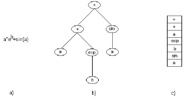
Figure 2.1: A mathematical expression in infix form (a), Polish form (c) and the corresponding program tree (b).

Each element in this vector contains a function or a terminal symbol. Since each function has a unique arity we can clearly interpret each vector that stores an expression in Polish notation. In this notation, a sub-tree of a program tree corresponds to a particular contiguous subsequence of the vector. When applying the crossover or the mutation operator, the exchanged or changed subsequences can easily be identified and manipulated.

2.2 Cartesian Genetic Programming

Cartesian Genetic Programming (CGP) [55] is a GP technique that encodes chromosomes in graph structures rather than standard GP trees. The motivation for this representation is that the graphs are more general than the tree structures, thus allowing the construction of more complex computer programs [55].

CGP is Cartesian in the sense that the graph nodes are represented in a Cartesian coordinate system. This representation was chosen due to the node connection mechanism, which is similar to GP mechanism. A CGP node contains a function symbol and pointers towards nodes representing function parameters. Each CGP node has an output that may be used as input for another node.

An example of CGP program is depicted in Figure 2.2.

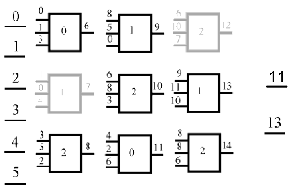
Figure 2.2: A CGP program with 5 inputs, 2 outputs and 3 functions (0, 1, 2 inside square nodes). The grey squares represent unconnected nodes.

Each CGP program (graph) is defined by several parameters: number of rows ($n_{r})$, number of columns ($n_{c})$, number of inputs, number of outputs, and number of functions. The nodes interconnectivity is defined as being the number ($l)$ of previous columns of cells that may have their outputs connected to a node in the current column (the primary inputs are treated as node outputs).

CGP chromosomes are encoded as strings by reading the graph columns top down and printing the input nodes and the function symbol for each node. The CGP chromosome depicted in Figure 2.2 is encoded as:

$C$ = 0 1 3 0 1 0 4 1 3 5 2 2 8 5 0 1 6 8 3 2 4 2 6 0 6 10 7 2 9 11 10 1 8 8 6 2 11 13

Standard string genetic operators (crossover and mutation) are used within CGP system. Crossover may be applied without any restrictions. Mutation operator requires that some conditions are met. Nodes supplying the outputs are not fixed as they are also subject to crossover and mutation.

2.3 Gene Expression Programming

Gene Expression Programming (GEP) [23] uses linear chromosomes. A chromosome is composed of genes containing terminal and function symbols. Chromosomes are modified by mutation, transposition, root transposition, gene transposition, gene recombination, one-point and two-point recombination.

GEP genes are composed of a head and a tail. The head contains both functions and terminals symbols. The tail contains only terminal symbols.

For each problem the head length ($h$) is chosen by the user. The tail length (denoted $t)$ is calculated using the formula:

$t=(n-1)*h+1$,

where $n$ is the number of arguments of the function with more arguments.

A tree-program is translated into a GEP gene is by means of breadth-first parsing.

Let us consider a gene made up of symbols in the set $S$:

$S$ = {*, /, +, -, $a$, $b$}.

In this case we have $n$ = 2. If we choose $h$ = 10 we get $t$ = 11, and the length of the gene is 10 + 11 = 21. Such a gene is given below:

$C$ = +*ab/+aab+ababbbababb.

The expression encoded by the gene $C$ is:

$E=(a+b)/a*b+a$.

The expression $E$ represents the phenotypic transcription of a chromosome having $C$ as its unique gene.

Usually, a GEP gene is not entirely used for phenotypic transcription. If the first symbol in the gene is a terminal symbol, the expression tree consists of a single node. If all symbols in the head are function symbols, the expression tree uses all the symbols of the gene.

GEP genes may be linked by a function symbol in order to obtain a fully functional chromosome. In the current version of GEP, the linking functions for algebraic expressions are addition and multiplication. A single type of function is used for linking multiple genes.

This seems to be enough in some situation [23]. But, generally, it is not a good idea to assume that the genes may be linked either by addition or by multiplication. If the functions {+, -, *, /} are used as linking operators then, the complexity of the problem grows substantially (since the problem of determining how to mixed these operators with the genes is as hard as the initial problem).

When solving computationally difficult problems (like automated code generation) one should not assume that a unique kind of function symbol (like for, while or if instructions) is necessary for inter-connecting different program parts.

Moreover, the success rate of GEP increases with the number of genes in the chromosome [23]. However, after a certain value, the success rate decreases if the number of genes in the chromosome increases. This is because one can not force a complex chromosome to encode a less complex expression.

Thus, when using GEP one must be careful with the number of genes that form the chromosome. The number of genes in the chromosome must be somehow related to the complexity of the expression that one wants to discover.

According to [23], GEP performs better than standard GP for several particular problems.

2.4 Linear Genetic Programming

Linear Genetic Programming (LGP) [9, 10, 11] uses a specific linear representation of computer programs. Instead of the tree-based GP expressions of a functional programming language (like LISP), programs of an imperative language (like C) are evolved.

A LGP individual is represented by a variable-length sequence of simple C language instructions. Instructions operate on one or two indexed variables (registers) $r$ or on constants $c$ from predefined sets. The result is assigned to a destination register, e.g. $r_{i}=r_{j}$ * $c$.

An example of the LGP program is the following one:

void LGP(double v[8])

{

v[0] = v[5] + 73;

v[7] = v[3] - 59;

if (v[1] $>$ 0)

if (v[5] $>$ 21)

v[4] = v[2] * v[1];

v[2] = v[5] + v[4];

v[6] = v[7] * 25;

v[6] = v[4] - 4;

v[1] = sin(v[6]);

if (v[0] $>$ v[1])

v[3] = v[5] * v[5];

v[7] = v[6] * 2;

v[5] = [7] + 115;

if (v[1] $<=$ v[6])

v[1] = sin(v[7]);

}

A linear genetic program can be turned into a functional representation by successive replacements of variables starting with the last effective instruction. The variation operators used here are crossover and mutation. By crossover, continuous sequences of instructions are selected and exchanged between parents. Two types of mutations are used: micro mutation and macro mutation. By micro mutation an operand or an operator of an instruction is changed. Macro mutation inserts or deletes a random instruction.

2.5 Grammatical Evolution

Grammatical Evolution (GE) [82] uses Backus - Naur Form (BNF) in order to express computer programs. BNF is a notation that allows a computer program to be expressed as a grammar.

A BNF grammar consists of terminal and non-terminal symbols. Grammar symbols may be re-written in other terminal and non-terminal symbols.

Each GE individual is a variable length binary string that contains the necessary information for selecting a production rule from a BNF grammar in its codons (groups of 8 bits).

An example from a BNF grammar is given by the following production rules:

$S$ ::= expr (0)

$|$if-stmt (1)

$|$loop (2)

These production rules state that the start symbol $S$ can be replaced (re-written) either by one of the non-terminals expr, if-stmt, or by loop.

The grammar is used in a generative process to construct a program by applying production rules, selected by the genome, beginning with the start symbol of the grammar.

In order to select a GE production rule, the next codon value on the genome is generated and placed in the following formula:

Rule = Codon_Value MOD Num_Rules.

If the next Codon integer value is 4, knowing that we have 3 rules to select from, as in the example above, we get 4 MOD 3 = 1.

Therefore, $S$ will be replaced with the non-terminal if-stmt, corresponding to the second production rule.

Beginning from the left side of the genome codon, integer values are generated and used for selecting rules from the BNF grammar, until one of the following situations arises:

• A complete program is generated. This occurs when all the non-terminals in the expression being mapped, are turned into elements from the terminal set of the BNF grammar.

• The end of the genome is reached, in which case the wrapping operator is invoked. This results in the return of the genome reading frame to the left side of the genome once again. The reading of the codons will then continue unless a higher threshold representing the maximum number of wrapping events has occurred during this individual mapping process.

In the case that a threshold on the number of wrapping events is exceeded and the individual is still incompletely mapped, the mapping process is halted, and the individual is assigned the lowest possible fitness value.

Example

Consider the grammar:

$G$ = {$N$, $T$, $S$, $P$},

where the terminal set is:

$T$ = {+, -, *, /, sin, exp, var, (, )},

and the nonterminal symbols are:

$N$ = {expr, op, pre_op}.

The start symbol is $S$ = $<$expr$>$.

The production rules $P$ are:

$<$expr$>$ :: $<$expr$>$ $<$op$>$ $<$expr$>$ $|$ (0)

($<$expr$>$ $<$op$>$ $<$expr$>$) $|$ (1)

$<$pre_op$>$ ($<$expr$>$) $|$ (2)

$<$var$>$. (3)

$<$op$>$ ::= + $|$ (0)

- $|$ (1)

* $|$ (2)

/. (3)

$<$pre_op$>$ ::= sin $|$ (0)

exp. (1)

An example of a GE chromosome is the following:

$C_{GE}$ = 000000000000001000000001000000110000001000000011.

Translated into GE codons, the chromosome is:

$C_{GE}$ = 0, 2, 1, 3, 2, 3.

This chromosome is translated into the expression:

$E$ = exp($x)$ * $x$.

Using the BNF grammars for specifying a chromosome provides a natural way of evolving programs written in programming languages whose instructions may be expressed as BNF rules.

The wrapping operator provides a very original way of translating short chromosomes into very long expressions. Wrapping also provides an efficient way to avoid the obtaining of invalid expressions.

The GE mapping process also has some disadvantages. Wrapping may never end in some situations. For instance consider the G_GE grammar defined above. In these conditions the chromosome

$C^{\prime}_{GE}$ = 0, 0, 0, 0, 0

cannot be translated into a valid expression as it does not contain operands. To prevent infinite cycling a fixed number of wrapping occurrences is allowed. If this threshold is exceeded the obtained expression is incorrect and the corresponding individual is considered to be invalid.

Since the debate regarding the supremacy of binary encoding over integer encoding has not finished yet we cannot say which one is better. However, as the translation from binary representations to integer/real representations takes some time we suspect that the GE system is a little slower than other GP techniques that use integer representation. GE uses a steady-state [95] algorithm.

Chapter 3 Multi Expression Programming

The chapter is organized as follows: MEP algorithm is given in section 3.2. Individual representation is described in section 3.3. The way in which MEP individuals are translated in computer programs is presented in section 3.4. The search operators used in conjunction with MEP are given in section 3.6. The way in which MEP handles exceptions raised during the fitness assignment process is presented in section 3.7. MEP complexity is computed in section 3.8.

The chapter is entirely original and it is based on the papers [64, 66, 65, 71, 79, 78].

3.1 MEP basic ideas

Multi Expression Programming (MEP) [64] is a GP variant that uses a linear representation of chromosomes. MEP individuals are strings of genes encoding complex computer programs.

When MEP individuals encode expressions, their representation is similar to the way in which compilers translate $C$ or Pascal expressions into machine code [2]. This may lead to very efficient implementation into assembler languages. The ability of evolving machine code (leading to very important speedups) has been considered by others researchers, too. For instance Nordin [62] evolves programs represented in machine code. Poli and Langdon [85] proposed Sub-machine code GP, which exploits the processor ability to perform some operations simultaneously. Compared to these approaches, MEP has the advantage that it uses a representation that is more compact, simpler, and independent of any programming language.

A salient MEP feature is the ability of storing multiple solutions of a problem in a single chromosome. Usually, the best solution is chosen for fitness assignment. When solving symbolic regression or classification problems (or any other problems for which the training set is known before the problem is solved) MEP has the same complexity as other techniques storing a single solution in a chromosome (such as GP, CGP, GEP or GE).

Evaluation of the expressions encoded into a MEP individual can be performed by a single parsing of the chromosome.

Offspring obtained by crossover and mutation are always syntactically correct MEP individuals (computer programs). Thus, no extra processing for repairing newly obtained individuals is needed.

3.2 MEP algorithm

Standard MEP algorithm uses steady-state evolutionary model [95] as its underlying mechanism.

The MEP algorithm starts by creating a random population of individuals. The following stpng are repeated until a given number of generations is reached: Two parents are selected using a standard selection procedure. The parents are recombined in order to obtain two offspring. The offspring are considered for mutation. The best offspring $O$ replaces the worst individual $W$ in the current population if $O$ is better than $W$.

The variation operators ensure that the chromosome length is a constant of the search process. The algorithm returns as its answer the best expression evolved along a fixed number of generations.

The standard MEP algorithm is outlined below:

Standard MEP Algorithm

S₁. Randomly create the initial population P(0)

S₂. for t = 1 to Max_Generations do

S₃. for k = 1 to $|$P(t)$|$ / 2 do

S₄. p₁ = Select(P(t)); // select one individual from the current

// population

S₅. p₂ = Select(P(t)); // select the second individual

S₆. Crossover (p₁, p₂, o₁, o₂); // crossover the parents p₁ and p₂

// the offspring o₁ and o₂ are obtained

S₇. Mutation (o₁); // mutate the offspring o₁

S₈. Mutation (o₂); // mutate the offspring o₂

S₉. if Fitness(o₁) $<$ Fitness(o₂)

S₁₀. then if Fitness(o₁) $<$ the fitness of the worst individual

in the current population

S₁₁. then Replace the worst individual with o₁;

S₁₂. else if Fitness(o₂) $<$ the fitness of the worst individual

in the current population

S₁₃. then Replace the worst individual with o₂;

S₁₄. endfor

S₁₅. endfor

3.3 MEP representation

MEP genes are (represented by) substrings of a variable length. The number of genes per chromosome is constant. This number defines the length of the chromosome. Each gene encodes a terminal or a function symbol. A gene that encodes a function includes pointers towards the function arguments. Function arguments always have indices of lower values than the position of the function itself in the chromosome.

The proposed representation ensures that no cycle arises while the chromosome is decoded (phenotypically transcripted). According to the proposed representation scheme, the first symbol of the chromosome must be a terminal symbol. In this way, only syntactically correct programs (MEP individuals) are obtained.

Example

Consider a representation where the numbers on the left positions stand for gene labels. Labels do not belong to the chromosome, as they are provided only for explanation purposes.

For this example we use the set of functions:

$F$ = {+, *},

and the set of terminals

$T$ = {$a$, $b$, $c$, $d$}.

An example of chromosome using the sets $F$ and $T$ is given below:

1: $a$

2: $b$

3: + 1, 2

4: $c$

5: $d$

6: + 4, 5

7: * 3, 6

The maximum number of symbols in MEP chromosome is given by the formula:

Number_of_Symbols = ($n+$1) * (Number_of_Genes – 1) + 1,

where $n$ is the number of arguments of the function with the greatest number of arguments.

The maximum number of effective symbols is achieved when each gene (excepting the first one) encodes a function symbol with the highest number of arguments. The minimum number of effective symbols is equal to the number of genes and it is achieved when all genes encode terminal symbols only.

3.4 MEP phenotypic transcription. Fitness assignment

Now we are ready to describe how MEP individuals are translated into computer programs. This translation represents the phenotypic transcription of the MEP chromosomes.

Phenotypic translation is obtained by parsing the chromosome top-down. A terminal symbol specifies a simple expression. A function symbol specifies a complex expression obtained by connecting the operands specified by the argument positions with the current function symbol.

For instance, genes 1, 2, 4 and 5 in the previous example encode simple expressions formed by a single terminal symbol. These expressions are:

$E_{1}=a$,

$E_{2}=b$,

$E_{4}=c$,

$E_{5}=d$,

Gene 3 indicates the operation + on the operands located at positions 1 and 2 of the chromosome. Therefore gene 3 encodes the expression:

$E_{3}=a+b$.

Gene 6 indicates the operation + on the operands located at positions 4 and 5. Therefore gene 6 encodes the expression:

$E_{6}=c+d$.

Gene 7 indicates the operation * on the operands located at position 3 and 6. Therefore gene 7 encodes the expression:

$E_{7}=(a+b)*(c+d)$.

$E_{7}$ is the expression encoded by the whole chromosome.

There is neither practical nor theoretical evidence that one of these expressions is better than the others. Moreover, Wolpert and McReady [100, 101] proved that we cannot use the search algorithm’s behavior so far for a particular test function to predict its future behavior on that function. This is why each MEP chromosome is allowed to encode a number of expressions equal to the chromosome length (number of genes). The chromosome described above encodes the following expressions:

$E_{1}=a$,

$E_{2}=b$,

$E_{3}=a+b$,

$E_{4}=c$,

$E_{5}=d$,

$E_{6}=c+d$,

$E_{7}$ = ($a+b)$ * ($c+d)$.

The value of these expressions may be computed by reading the chromosome top down. Partial results are computed by dynamic programming [7] and are stored in a conventional manner.

Due to its multi expression representation, each MEP chromosome may be viewed as a forest of trees rather than as a single tree, which is the case of Genetic Programming.

As MEP chromosome encodes more than one problem solution, it is interesting to see how the fitness is assigned.

The chromosome fitness is usually defined as the fitness of the best expression encoded by that chromosome.

For instance, if we want to solve symbolic regression problems, the fitness of each sub-expression $E_{i}$ may be computed using the formula:

$$f(E_{i})=\sum\limits_{k=1}^{n}{\left|{o_{k,i}-w_{k}}\right|},$$ (3.1)

where $o_{k,i}$ is the result obtained by the expression $E_{i}$ for the fitness case $k$ and $w_{k}$ is the targeted result for the fitness case $k$. In this case the fitness needs to be minimized.

The fitness of an individual is set to be equal to the lowest fitness of the expressions encoded in the chromosome:

$$f(C)=\mathop{\min}\limits_{i}f(E_{i}).$$ (3.2)

When we have to deal with other problems, we compute the fitness of each sub-expression encoded in the MEP chromosome. Thus, the fitness of the entire individual is supplied by the fitness of the best expression encoded in that chromosome.

3.5 MEP representation revisited

Generally a GP chromosome encodes a single expression (computer program). This is also the case for GEP and GE chromosomes. By contrast, a MEP chromosome encodes several expressions (as it allows a multi-expression representation). Each of the encoded expressions may be chosen to represent the chromosome, i.e. to provide the phenotypic transcription of the chromosome. Usually, the best expression that the chromosome encodes supplies its phenotypic transcription (represents the chromosome).

Therefore, the MEP technique is based on a special kind of implicit parallelism. A chromosome usually encodes several well-defined expressions. The ability of MEP chromosome to encode several syntactically correct expressions in a chromosome is called strong implicit parallelism (SIP).

Although, the ability of storing multiple solutions in a single chromosome has been suggested by others authors, too (see for instance [49]), and several attempts have been made for implementing this ability in GP technique. For instance Handley [37] stored the entire population of GP trees in a single graph. In this way a lot of memory is saved. Also, if partial solutions are efficiently stored, we can get a considerable speed up.

Linear GP [9] is also very suitable for storing multiple solutions in a single chromosome. In that case the multi expression ability is given by the possibility of choosing any variable as the program output.

It can be seen that the effective length of the expression may increases exponentially with the length of the chromosome. This is happening because some sub-expressions may be used more than once to build a more complex (or a bigger) expression. Consider, for instance, that we want to obtain a chromosome that encodes the expression$a^{2^{n}}$, and only the operators {+, -, *, /} are allowed. If we use a GEP representation the chromosome has to contain at least (2ⁿ⁺¹– 1) symbols since we need to store 2ⁿ terminal symbols and (2ⁿ – 1) function operators. A GEP chromosome that encodes the expression $E=a^{8}$ is given below:

$C$ = *******aaaaaaaa.

A MEP chromosome uses only (3$n$ + 1) symbols for encoding the expression $a^{2^{n}}$. A MEP chromosome that encodes expression $E=a^{8}$ is given below:

1: $a$

2: * 1, 1

3: * 2, 2

4: * 3, 3

As a further comparison, when $n$ = 20, a GEP chromosome has to have 2097151 symbols, while MEP needs only 61 symbols.

MEP representation is similar to GP and CGP, in the sense that each function symbol provides pointers towards its parameters. Whereas both GP and CGP have complicated representations (trees and graphs), MEP provides an easy and effective way to connect (sub) parts of a computer program. Moreover, the motivation for MEP was to provide an individual representation close to the way in which C or Pascal compilers interpret mathematical expressions [2]. That code is also called three addresses code or intermediary code.

Some GP techniques, like Linear GP, remove non-coding sequences of chromosome during the search process. As already noted [9] this strategy does not give the best results. The reason is that sometimes, a part of the useless genetic material has to be kept in the chromosome in order to maintain population diversity.

3.6 Search operators

The search operators used within MEP algorithm are crossover and mutation. These search operators preserve the chromosome structure. All offspring are syntactically correct expressions.

3.6.1 Crossover

By crossover two parents are selected and are recombined.

Three variants of recombination have been considered and tested within our MEP implementation: one-point recombination, two-point recombination and uniform recombination.

One-point recombination

One-point recombination operator in MEP representation is similar to the corresponding binary representation operator [19]. One crossover point is randomly chosen and the parent chromosomes exchange the sequences at the right side of the crossover point.

Example

Consider the parents $C_{1}$ and $C_{2}$ given below. Choosing the crossover point after position 3 two offspring, $O_{1}$ and $O_{2}$ are obtained as given in Table 3.1.

Table 3.1: MEP one-point recombination.

Parents		Offspring
$C_{1}$	$C_{2}$	$O_{1}$	$O_{2}$
1: b 2: * 1, 1 3: + 2, 1 4: a 5: * 3, 2 6: a 7: - 1, 4	1: $a$ 2: $b$ 3: + 1, 2 4: $c$ 5: $d$ 6: + 4, 5 7: * 3, 6	1: b 2: * 1, 1 3: + 2, 1 4: $c$ 5: $d$ 6: + 4, 5 7: * 3, 6	1: $a$ 2: $b$ 3: + 1, 2 4: a 5: * 3, 2 6: a 7: - 1, 4

Two-point recombination

Two crossover points are randomly chosen and the chromosomes exchange genetic material between the crossover points.

Example

Let us consider the parents $C_{1}$ and $C_{2}$ given below. Suppose that the crossover points were chosen after positions 2 and 5. In this case the offspring $O_{1}$ and $O_{2}$ are obtained as given in Table 3.2.

Table 3.2: MEP two-point recombination.

Parents		Offspring
$C_{1}$	$C_{2}$	$O_{1}$	$O_{2}$
1: b 2: * 1, 1 3: + 2, 1 4: a 5: * 3, 2 6: a 7: - 1, 4	1: $a$ 2: $b$ 3: + 1, 2 4: $c$ 5: $d$ 6: + 4, 5 7: * 3, 6	1: b 2: * 1, 1 3: + 1, 2 4: $c$ 5: $d$ 6: a 7: - 1, 4	1: $a$ 2: $b$ 3: + 2, 1 4: a 5: * 3, 2 6: + 4, 5 7: * 3, 6

Uniform recombination

During the process of uniform recombination, offspring genes are taken randomly from one parent or another.

Example

Let us consider the two parents $C_{1}$ and $C_{2}$ given below. The two offspring $O_{1}$ and $O_{2}$ are obtained by uniform recombination as given in Table 3.3.

Table 3.3: MEP uniform recombination.

Parents		Offspring
$C_{1}$	$C_{2}$	$O_{1}$	$O_{2}$
1: b 2: * 1, 1 3: + 2, 1 4: a 5: * 3, 2 6: a 7: - 1, 4	1: $a$ 2: $b$ 3: + 1, 2 4: $c$ 5: $d$ 6: + 4, 5 7: * 3, 6	1: $a$ 2: * 1, 1 3: + 2, 1 4: $c$ 5: * 3, 2 6: + 4, 5 7: - 1, 4	1: b 2: $b$ 3: + 1, 2 4: a 5: $d$ 6: a 7: * 3, 6

It is easy to derive - by analogy with standard GA several recombination operators.

3.6.2 Mutation

Each symbol (terminal, function of function pointer) in the chromosome may be the target of the mutation operator. Some symbols in the chromosome are changed by mutation. To preserve the consistency of the chromosome, its first gene must encode a terminal symbol.

We may say that the crossover operator occurs between genes and the mutation operator occurs inside genes.

If the current gene encodes a terminal symbol, it may be changed into another terminal symbol or into a function symbol. In the later case, the positions indicating the function arguments are randomly generated. If the current gene encodes a function, the gene may be mutated into a terminal symbol or into another function (function symbol and pointers towards arguments).

Example

Consider the chromosome $C$ given below. If the boldfaced symbols are selected for mutation an offspring $O$ is obtained as given in Table 3.4.

Table 3.4: MEP mutation.

$C$	$O$
1: $a$ 2: * 1, 1 3: b 4: * 2, 2 5: $b$ 6: + 3, 5 7: $a$	1: $a$ 2: * 1, 1 3: + 1, 2 4: * 2, 2 5: $b$ 6: + 1, 5 7: $a$

3.7 Handling exceptions within MEP

Exceptions are special situations that interrupt the normal flow of expression evaluation (program execution). An example of exception is division by zero, which is raised when the divisor is equal to zero.

Exception handling is a mechanism that performs special processing when an exception is thrown.

Usually, GP techniques use a protected exception handling mechanism [42]. For instance, if a division by zero exception is encountered, a predefined value (for instance 1 or the numerator) is returned.

GEP uses a different mechanism: if an individual contains an expression that generates an error, this individual receives the lowest fitness possible [23].

MEP uses a new and specific mechanism for handling exceptions. When an exception is encountered (which is always generated by a gene containing a function symbol), the gene that generated the exception is mutated into a terminal symbol. Thus, no infertile individual appears in a population.

3.8 MEP complexity

Let NG be the number of genes in a chromosome.

When solving symbolic regression, classification or any other problems for which the training set is known in advance (before computing the fitness), the fitness of an individual can be computed in O(NG) stpng by dynamic programming [7]. In fact, a MEP chromosome needs to be read once for computing the fitness.

Thus, MEP decoding process does not have a higher complexity than other GP - techniques that encode a single computer program in each chromosome.

3.9 Conclusions

Multi Expression Programming has been described in this chapter. A detailed description of the representation and of the fitness assignment has been given.

A distinct feature of MEP is its ability to encode multiple solutions in the same chromosome. It has been shown that the complexity of decoding process is the same as in the case of other GP techniques encoding a single solution in the same chromosome.

Chapter 4 MEP for Data Mining

4.1 Introduction

Multi Expression Programming is used for solving several symbolic regression and classification problems. A comparison of MEP with standard GP, GEP and CGP is also provided.

The chapter is organized as follows: Symbolic regression problems are addressed in section 4.2. For this problem MEP is compared to GP, GEP and CGP. Even Parity problems are addressed in section 5.1. The Multiplexer is addressed in section 5.2. The way in which MEP may be used for designing digital circuits is described in sections 5.3 and 5.4. In sections 6.1 and 6.2 MEP is used to evolve winning strategies for the Tic-Tac-Toe and Nim-like games. Another interesting application of MEP is the discovery of heuristics for NP-Complete problems. In section 6.3 MEP is used for evolving an heuristic for the Traveling Salesman Problem.

The chapter is based on the author’s papers [64].

4.2 Symbolic regression

In this section, MEP technique is used for solving symbolic regression problems. Results are reported in the papers [64].

4.2.1 Problem statement

The aim of symbolic regression is to discover a function that satisfies a set of fitness cases.

Two well-known problems are used for testing the MEP ability of solving symbolic regression problems. The problems are:

The quartic polynomial [42]. Find a mathematical expression that satisfies best a set of fitness cases generated by the function:

$f(x)=x^{4}+x^{3}+x^{2}+x$.

The sextic polynomial [43]. Find a mathematical expression that satisfies best a set of fitness cases generated by the function:

$f(x)=x^{6}-2x^{4}+x^{2}$.

A set of 20 fitness cases was randomly generated over the interval [-1.0, 1.0] and used in the experiments performed.

4.2.2 Numerical experiments

In this section several numerical experiments with Multi Expression Programming for solving symbolic regression problems are performed.

Experiment 1

The success rate of the MEP algorithm is analyzed in this experiment. Success rate is computed as the number of successful runs over the total number of runs. The chromosome length is gradually increased. MEP algorithm parameters are given in Table 4.1.

Table 4.1: Algorithm parameters for the Experiment 1.

Parameter	Value
Population size	30
Number of generations	50
Mutation	2 symbols / chromosome
Crossover type	Uniform-crossover
Crossover probability	0.9
Selection	Binary tournament
Terminal Set	$T$ = {$x$}
Function Set	$F$ = {+, -, *, /}

The success rate of the MEP algorithm depending on the number of symbols in the chromosome is depicted in Figure 4.1.

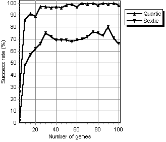
Figure 4.1: The relationship between the success rate and the number of symbols in a MEP chromosome. The number of symbols in chromosome varies between 5 and 100. The results are summed over 100 runs.

The success rate of the MEP algorithm increases with the chromosome length and never decreases towards very low values. When the search space (chromosome length) increases, an increased number of expressions are encoded by MEP chromosomes. Very large search spaces (very long chromosomes) are extremely beneficial for MEP technique due to its multi expression representation. This behavior is different from those obtained with the GP variants that encode a single solution in a chromosome (such as GEP). Figure 4.1 also shows that the sextic polynomial is more difficult to solve with MEP (with the parameters given in Table 4.1) than the quatic polynomial.

Experiment 2

From Experiment 1 we may infer that for the considered problem, the MEP success rate never decreases to very low values as the number of genes increases. To obtain an experimental evidence for this assertion longer chromosomes are considered. We extend chromosome length up to 300 genes (898 symbols).

The success rate of MEP is depicted in Figure 4.2.

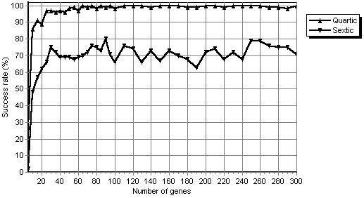
Figure 4.2: The relationship between the success rate and the number of symbols in a MEP chromosome. The number of symbols in chromosome varies between 5 and 300. The results are summed over 100 runs.

Figure 4.2 shows that, when solving the quartic (sextic) polynomial problem, the MEP success rate, lies in the interval [90, 100] ([60, 80]) for the chromosome length larger than 20.

One may note that after that the chromosome length becomes 10, the success rate never decrease more than 90% (for the quartic polynomial) and never decrease more than 60% (for the sextic polynomial). It also seems that, after a certain value of the chromosome length, the success rate does not improve significantly.

Experiment 3

In this experiment the relationship between the success rate and the population size is analyzed. Algorithm parameters for this experiment are given in Table 4.2.

Table 4.2: Algorithm parameters for Experiment 3.

Parameter	Value
Number of generations	50
Chromosome length	10 genes
Mutation	2 symbols / chromosome
Crossover type	Uniform-crossover
Crossover probability	0.9
Selection	Binary tournament
Terminal Set	$T$ = {$x$}
Function Set	$F$ = {+, -, *, /}

Experiment results are given in Figure 4.3.

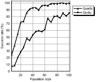
Figure 4.3: Success rate of the MEP algorithm. Population size varies between 5 and 100. The results are summed over 100 runs.

For the quartic problem and for the MEP algorithm parameters given in Table 4.2, the optimal population size is 70 (see Figure 4.3). The corresponding success rate is 99%. A population of 100 individuals yields a success rate of 88% for the sextic polynomial. This result suggests that even small MEP populations may supply very good results.

Experiment 4

In this experiment the relationship between the MEP success rate and the number of generations used in the search process is analyzed.

MEP algorithm parameters are given in Table 4.3.

Table 4.3: Algorithm parameters for Experiment 4.

Parameter	Value
Population size	20
Chromosome length	12 genes
Mutation	2 genes / chromosome
Crossover type	Uniform-crossover
Crossover probability	0.9
Selection	Binary tournament
Terminal Set	$T$ = {$x$}
Function Set	$F$ = {+, -, *, /}

Experiment results are given in Figure 4.4.

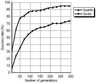
Figure 4.4: Relationship between the success rate of MEP algorithm and the number of generations used in the search process. The number of generations varies between 10 and 300. The results are summed over 100 runs.

Figure 4.4 shows that the success rate of the MEP algorithm rapidly increases from 34%, respectively 8% (when the number of generations is 10) up to 95%, and 74% respectively (when the number of generations is 300).

4.2.3 MEP vs. GEP

In [23] GEP has been used for solving the quartic polynomial based on a set of 10 fitness cases randomly generated over the interval [0, 20]. Several numerical experiments analyzing the relationship between the success rate and the main parameters of the GEP algorithm have been performed in [23]. In what follows we will perform similar experiments with MEP.

The first experiment performed in [23] analyses the relationship between the GEP chromosome length and the success rate. GEP success rate increases up to 80% (obtained when the GEP chromosome length is 30) and then decreases. This indicates that very long GEP chromosomes cannot encode short expressions efficiently. The length of the GEP chromosome must be somehow related to the length of the expression that must be discovered.

Using the same parameter setting (i.e. Population Size = 30, Number of Generations = 50; Crossover probability = 0.7, Mutations = 2 / chromosome), the MEP obtained a success rate of 98% when the chromosome length was set to 20 genes (58 symbols).

The second experiment performed in [23] analyses the relationship between the population size used by the GEP algorithm and the success rate. For a population of size 30, the GEP success rate reaches 80%, and for a population of 50 individuals the GEP success rate reaches 90%.

Using the same parameter setting (i.e. Number of Symbols in Chromosome = 49 (17 MEP genes), Number of Generations = 50; Crossover probability = 0.7, Mutations = 2 / chromosome), MEP obtained a success rate of 99% (in 99 runs out of 100 MEP has found the correct solution) using a population of only 30 individuals.

In another experiment performed in [23], the relationship between the number of generations used by GEP and the rate of success is analysed. The success rate of 69% was obtained by GEP when the number of generations was 70 and a success rate of 90% was obtained only when the number of generations reached 500. For the considered generation range GEP success rate never reached 100%.

Using the same parameter setting (i.e. Number of Symbols in Chromosome = 80 (27 MEP genes), Population Size = 30; Crossover probability = 0.7, Mutations = 2 / chromosome), the MEP obtained a success rate of 97% (in 97 runs out of 100 MEP has found the correct solution) using 30 generations only. This is an improvement (regarding the number of generations used to obtain the same success rate) with more than one order of magnitude.

We may conclude that for the quartic polynomial, the MEP has a higher success rate than GEP using the previously given parameter settings.

4.2.4 MEP vs. CGP

CGP has been used [55] for symbolic regression of the sextic polynomial problem.

In this section, the MEP technique is used to solve the same problem using parameters settings similar to those of CGP. To provide a fair comparison, all experimental conditions described in [55] are carefully reproduced for the MEP technique.

CGP chromosomes were characterized by the following parameters: $n_{r}$ = 1, $n_{c}$ = 10, $l$ = 10. MEP chromosomes are set to contain 12 genes (in addition MEP uses two supplementary genes for the terminal symbols {1.0, $x$}).

MEP parameters (similar to those used by CGP) are given in Table 4.4.

Table 4.4: Algorithm parameters for the MEP vs. CGP experiment.

Parameter	Value
Chromosome length	12 genes
Mutation	2 genes / chromosome
Crossover type	One point crossover
Crossover probability	0.7
Selection	Binary tournament
Elitism size	1
Terminal set	$T$ = {$x$, 1.0}
Function set	$F$ = {+, -, *, /}

In the experiment with CGP a population of 10 individuals and a number of 8000 generations have been used. We performed two experiments. In the first experiment, the MEP population size is set to 10 individuals and we compute the number of generations needed to obtain the success rate (61 %) reported in [55] for CGP.

When the MEP run for 800 generations, the success rate was 60% (in 60 runs (out of 100) MEP found the correct solution). Thus MEP requires 10 times less generations than CGP to solve the same problem (the sextic polynomial problem in our case). This represents an improvement of one order of magnitude.

In the second experiment, the number of generations is kept unchanged (8000) and a small MEP population is used. We are interested to see which is the optimal population size required by MEP to solve this problem.

After several trials, we found that MEP has a success rate of 70% when a population of 3 individuals is used and a success rate of 46% when a population of 2 individuals is used. This means that MEP requires 3 times less individuals than CGP for solving the sextic polynomial problem.

4.2.5 MEP vs. GP

In [42] GP was used for symbolic regression of the quartic polynomial function.

GP parameters are given in Table 4.5.

Table 4.5: GP parameters used for solving the quartic problem.

Parameter	Value
Population Size	500
Number of generations	51
Crossover probability	0.9
Mutation probability	0
Maximum tree depth	17
Maximum initial tree depth	6
Terminal set	$T$ = {$x$}
Function set	$F$ = {+, - , *, %, Sin, Cos, Exp, RLog}

It is difficult to compare MEP with GP since the experimental conditions were not the same. The main difficulty is related to the number of symbols in chromosome. While GP individuals may increase, MEP chromosomes have fixed length. Individuals in the initial GP population are trees having a maximum depth of 6 levels. The number of nodes in the largest tree containing symbols from $F\quad\cup\quad T$ and having 6 levels is 2⁶ – 1 = 63 nodes. The number of nodes in the largest tree containing symbols from $F\quad\cup\quad T$ and having 17 levels (maximum depth allowed for a GP tree) is 2¹⁷ – 1 = 131071 nodes.

Due to this reason we cannot compare MEP and GP relying on the number of genes in a chromosome. Instead, we analyse different values for the MEP chromosome length.

MEP algorithm parameters are similar to those used by GP [42]. The results are depicted in Figure 4.5.

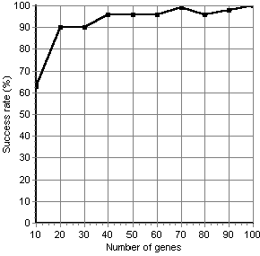
Figure 4.5: The relationship between the number of genes in a chromosome and the MEP success rate. The number of genes in a chromosome varies between 10 and 100. The results are averaged over 100 runs.

For this problem, the GP cumulative probability of success is 35% (see [42]). Figure 4.5 shows that the lowest success rate for MEP is 65%, while the highest success rate is 100% (for the considered chromosome length domain). Thus, MEP outperforms GP on the quartic polynomial problem (when the parameters given in Table 4.1 are used).

4.3 Conclusions

In this chapter, MEP has been used for solving various symbolic regression problems. MEP has been compared with other Genetic Programming techniques. Numerical results indicate that MEP performs better than the compared methods.

Chapter 5 Designing Digital Circuits with MEP

MEP is used for designing digital circuits based on the truth table. Four problems are addressed: even-parity, multiplexer, arithmetic circuits and circuits for NP-complete problems. This chapter is entirely original and it is based on the papers [66, 79, 80].

5.1 Even-parity problem

5.1.1 Problem statement

The Boolean even-parity function of $k$ Boolean arguments returns T (True) if an even number of its arguments are T. Otherwise the even-parity function returns NIL (False) [42].

In applying MEP to the even-parity function of $k$ arguments, the terminal set $T$ consists of the $k$ Boolean arguments $d_{0}$, $d_{1}$, $d_{2}$, … $d_{k-1}$. The function set $F$ consists of four two-argument primitive Boolean functions: AND, OR, NAND, NOR. According to [42] the Boolean even-parity functions appear to be the most difficult Boolean functions to be detected via a blind random search.

The set of fitness cases for this problem consists of the 2^k combinations of the $k$ Boolean arguments. The fitness of an MEP chromosome is the sum, over these 2^k fitness cases, of the Hamming distance (error) between the returned value by the MEP chromosome and the correct value of the Boolean function. Since the standardized fitness ranges between 0 and 2^k, a value closer to zero is better (since the fitness is to be minimized).

5.1.2 Numerical experiments

The parameters for the numerical experiments with MEP for even-parity problems are given in Table 5.1.

Table 5.1: The MEP algorithm parameters for the numerical experiments with even-parity problems.

Parameter	Value
Number of generations	51
Crossover type	Uniform
Crossover probability	0.9
Mutation probability	0.2
Terminal set	$T_{3}$ = {$D_{0},D_{1},D_{2}$} for even-3-parity $T_{4}$ = {$D_{0},D_{1},D_{2}$, $D_{3}$} for even-4-parity
Function set	$F$ = {AND, OR, NAND, NOR}

In order to reduce the length of the chromosome all the terminals are kept on the first positions of the MEP chromosomes. The selection pressure is also increased by using higher values (usually 10% of the population size) for the $q$-tournament size.

Several numerical experiments with MEP have been performed for solving the even-3-parity and the even-4-parity problems. After several trials we have found that a population of 100 individuals having 300 genes was enough to yield a success rate of 100% for the even-3-parity problem and a population of 400 individuals with 200 genes yielded a success rate of 43% for the even-4-parity problem. GP without Automatically Defined Functions has been used for solving the even-3 and even-4 parity problems using a population of 4000 individuals [42]. The cumulative probability of success was 100% for the even-3-parity problem and 42% for the even-4-parity problem [42]. Thus, MEP outperforms GP for the even-3 and even-4 parity problems with more than one order of magnitude. However, we already mentioned, a perfect comparison between MEP and GP cannot be drawn due to the incompatibility of the respective representations.

One of the evolved circuits for the even-3-parity problem is given in Figure 5.1 and one of the evolved circuits for the even-4-parity is given in Figure 5.2.

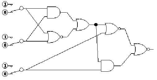
Figure 5.1: An evolved circuit for the even-3-parity problem.

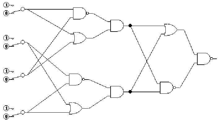
Figure 5.2: An evolved circuit for the even-4-parity problem.

5.2 Multiplexer problem

In this section, the MEP technique is used for solving the 6-multiplexer and the 11-multiplexer problems [42]. Numerical experiments obtained by applying MEP to multiplexer problem are reported in [64].

5.2.1 Problem statement

The input to the Boolean $N$-multiplexer function consists of $k$ address bits $a_{i}$ and 2^k data bits $d_{i}$, where

$N=k$ + 2^k. That is, the input consists of the $k$+2^k bits $a_{k-1}$, … , $a_{1}$, $a_{0}$, $d_{2}k_{-1}$, … , $d_{1}$, $d_{0}$. The value of the Boolean multiplexer function is the Boolean value (0 or 1) of the particular data bit that is singled out by the $k$ address bits of the multiplexer. Another way to look at the search space is that the Boolean multiplexer function with $k$+2^k arguments is a particular function of $2^{k+2^{k}}$ possible Boolean functions of $k$+2^k arguments. For example, when $k$=3, then $k$+2^k = 11 and this search space is of size 22¹¹. That is, the search space is of size 2²⁰⁴⁸, which is approximately 10⁶¹⁶.

The terminal set for the 6-multiplexer problem consists of the 6 Boolean inputs, and for the 11-multiplexer problem consists of the 11 Boolean inputs. Thus, the terminal set $T$ for the 6-multiplexer is of $T$= {$a_{0}$, $a_{1}$, $d_{0}$, $d_{1}$, … , $d_{4}$} and for the 11-multiplexer is of $T$= {$a_{0}$, $a_{1}$, $a_{2}$, $d_{0}$, $d_{1}$, … , $d_{7}$}.

The function set $F$ for this problem is $F$ = {AND, OR, NOT, IF} taking 2, 2, 1, and 3 arguments, respectively [42]. The function IF returns its 3^rd argument if its first argument is set to 0. Otherwise it returns its second argument.

There are 2¹¹ = 2,048 possible combinations of the 11 arguments $a_{0}a_{1}a_{2}d_{0}d_{1}d_{2}d_{3}d_{4}d_{5}d_{6}d_{7}$ along with the associated correct value of the 11-multiplexer function. For this particular problem, we use the entire set of 2048 combinations of arguments as the fitness cases for evaluating fitness.

5.2.2 Numerical experiments

Several numerical experiments with the 6-multiplexer and 11-multiplexer are performed in this section.

Experiments with 6-multiplexer

Two main statistics are of high interest: the relationship between the success rate and the number of genes in a MEP chromosome and the relationship between the success rate and the size of the population used by the MEP algorithm. For these experiments the parameters are given in Table 5.2.

Table 5.2: MEP algorithm parameters for the numerical experiments with 6-multiplexer problem.

Parameter	Value
Number of generations	51
Crossover type	Uniform
Crossover probability	0.9
Mutation probability	0.1
Terminal set	$T$= {$a_{0}$, $a_{1}$, $d_{0}$, $d_{1}$, … , $d_{4}$}
Function set	$F$= {AND, OR, NOT, IF}

A population of 100 individuals is used when the influence of the number of genes is analysed and a code length of 100 genes is used when the influence of the population size is analysed. For reducing the chromosome length we keep all the terminals on the first positions of the MEP chromosomes. We also increased the selection pressure by using larger values (usually 10% of the population size) for the tournament sample.

The results of these experiments are given in Figure 5.3.

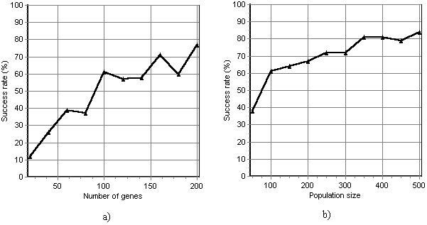
Figure 5.3: The success rate of the MEP algorithm for solving the 6-multiplexer problem. (a) The relationship between the success rate and the chromosome length. (b) The relationship between the success rate and the population size. Results are summed over 100 runs.

Figure 5.3 shows that MEP is able to solve the 6-multiplexer problem very well. A population of 500 individuals yields a success rate of 84%. A similar experiment using the GP technique with a population of 500 individuals has been reported in [83]. The reported probability of success is a little less (79,5%) than the one obtained with MEP (84%).

Experiments with 11-multiplexer

We also performed several experiments with the 11-multiplexer problem. We have used a population of 500 individuals and three values (100, 200 and 300) for the number of genes in a MEP chromosome. In all these experiments, MEP was able to find a perfect solution (out of 30 runs), thus yielding a success rate of 3.33%. When the number of genes was set to 300, the average of the best fitness of each run taken as a percentage of the perfect fitness was 91.13%, with a standard deviation of 4.04. As a comparison, GP was not able to obtain a perfect solution by using a population of 500 individuals and the average of the best fitness of each run taken as a percentage of the perfect fitness was 79.2% (as reported in [83]).

5.3 Designing digital circuits for arithmetic functions

The problem of evolving digital circuits has been intensely analyzed in the recent past [54, 56, 57, 58, 91]. A considerable effort has been spent on evolving very efficient (regarding the number of gates) digital circuits. J. Miller, one of the pioneers in the field of the evolvable digital circuits, used a special technique called Cartesian Genetic Programming (CGP) [55] for evolving digital circuits. CGP architecture consists of a network of gates (placed in a grid structure) and a set of wires connecting them. For instance this structure has been used for evolving digital circuits for the multiplier problem [58]. The results [58] shown that CGP was able to evolve digital circuits better than those designed by human experts.

In this section, we use Multi Expression Programming for evolving digital circuits with multiple outputs. We present the way in which MEP may be efficiently applied for evolving digital circuits. We show the way in which multiple digital circuits may be stored in a single MEP chromosome and the way in which the fitness of this chromosome may be computed by traversing the MEP chromosome only once.

Several numerical experiments are performed with MEP for evolving arithmetic circuits. The results show that MEP significantly outperforms CGP for the considered test problems.

Numerical results are reported in the papers [79].

5.3.1 Problem statement

The problem that we are trying to solve here may be briefly stated as follows:

Find a digital circuit that implements a function given by its truth table.

The gates that are usually used in the design of digital circuits along with their description are given in Table 5.3.

Table 5.3: Function set (gates) used in numerical experiments. Some functions are independent on the input (functions 0 and 1), other depend on only one of the input variables (functions 2-5), other functions depend on two input variables (functions 6-15) and the other functions depends on three input variables (functions 16-19). These functions are taken from [58].

#	Function	#	Function
0	0	10	$a\oplus b$
1	1	11	$a\oplus\bar{b}$
2	$a$	12	$a+b$
3	$b$	13	$a+\bar{b}$
4	$\bar{a}$	14	$\bar{a}+b$
5	$\bar{b}$	15	$\bar{a}+\bar{b}$
6	$a\cdot b$	16	$a\cdot\bar{c}+b\cdot c$
7	$a\cdot\bar{b}$	17	$a\cdot\bar{c}+\bar{b}\cdot c$
8	$\bar{a}\cdot b$	18	$\bar{a}\cdot\bar{c}+b\cdot c$
9	$\bar{a}\cdot\bar{b}$	19	$\bar{a}\cdot\bar{c}+\bar{b}\cdot c$

The symbols used to represent some of the logical gates are given in Figure 5.4.

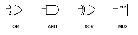
Figure 5.4: The symbols used to represent some of the logical gates in Table 5.3 (OR is function 12, AND is function 6, XOR is function 10 and MUX is function 16). In some pictures a small circle may appear on these symbols indicating the negation (inversion) of the respective results.

The MUX gate may be also represented using 2 ANDs and 1 OR [58]. However some modern devices use the MUX gate as an atomic device in that all other gates are synthesized using this one.

Gates may also be represented using the symbols given in Table 5.4.

Table 5.4: Representation of some functions given in Table 5.3.

Gate	Representation
AND	$\cdot$
OR	+
XOR	$\oplus$
NOT	-

5.3.2 CGP for evolving digital circuits

An example of CGP program encoding a digital circuit is depicted in Figure 5.5.

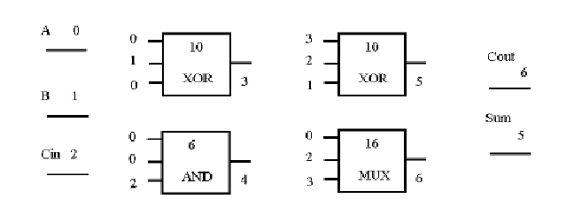
Figure 5.5: A Cartesian Genetic Programming program for 1-bit adder problem.

In Figure 5.5, a gate array representation of a one-bit adder is given. $A$, $B$, and Cin are the binary inputs. The outputs Sum and Cout are the binary outputs. Sum represents the sum bit of the addition of $A+B$+Cin, and Cout the carry bit. The chromosome representation of the circuit in Figure 2 is the following (function symbols are given in bold):

0 1 0 10 0 0 2 6 3 2 1 10 0 2 3 16 6 5.

The evolutionary algorithm used in [58] to evolve digital circuits is a simple form of (1+$\lambda)$-ES [19, 58], where $\lambda$ was set to 4. This algorithm seems to perform very well in conjunction to CGP representation. However, a Genetic Algorithm (GA) [34] may also be used as underlying mechanism for CGP.

5.3.3 MEP for evolving digital circuits

In this section we describe the way in which Multi Expression Programming may be efficiently used for evolving digital circuits.

Each circuit has one or more inputs (denoted by NI) and one or more outputs (denoted NO). In section 3.4 we presented the way in which is the fitness of a chromosome with a single output is computed. When multiple outputs are required for a problem, we have to choose NO genes which will provide the desired output (it is obvious that the genes must be distinct unless the outputs are redundant).

In CGP, the genes providing the program’s output are evolved just like all other genes. In MEP, the best genes in a chromosome are chosen to provide the program’s outputs. When a single value is expected for output we simply choose the best gene (see section 3.4). When multiple genes are required as outputs we have to select those genes which minimize the difference between the obtained result and the expected output.

We have to compute first the quality of a gene (sub-expression) for a given output:

$$f(E_{i},q)=\sum\limits_{k=1}^{n}{\left|{o_{k,i}-w_{k,q}}\right|},$$ (5.1)

where $o_{k,i}$ is the obtained result by the expression (gene) $E_{i}$ for the fitness case $k$ and $w_{k,q}$ is the targeted result for the fitness case $k$ and for the output $q$. The values $f(E_{i}$, $q)$ are stored in a matrix (by using dynamic programming [7] for latter use (see formula (5.2)).

Since the fitness needs to be minimized, the quality of a MEP chromosome is computed by using the formula:

$$f(C)=\mathop{\min}\limits_{i_{1},i_{2},...,i_{NO}}\sum\limits_{q=1}^{NO}{f(E_{i_{q}},q)}.$$ (5.2)

In equation (5.2) we have to choose numbers $i_{1}$, $i_{2}$, …, $i_{NO}$ in such way to minimize the program’s output. For this we shall use a simple heuristic which does not increase the complexity of the MEP decoding process: for each output $q$ (1 $\leq\quad q\quad\leq$ NO) we choose the gene $i$ that minimize the quantity $f(E_{i}$, $q)$. Thus, to an output is assigned the best gene (which has not been assigned before to another output). The selected gene will provide the value of the $q^{th}$ output.

Remark
Formulas (5.1) and (5.2) are the generalization of formulas (3.1) and (3.2) for the case of multiple outputs of a MEP chromosome.

The complexity of the heuristic used for assigning outputs to genes is

O(NG $\cdot$ NO)

where NG is the number of genes and NO is the number of outputs.

We may use another procedure for selecting the genes that will provide the problem’s outputs. This procedure selects, at each step, the minimal value in the matrix $f(E_{i}$, $q)$ and assign the corresponding gene $i$ to its paired output $q$. Again, the genes already used will be excluded from the search. This procedure will be repeated until all outputs have been assigned to a gene. However, we did not used this procedure because it has a higher complexity – $O$(NO$\cdot$log₂(NO)$\cdot$NG) - than the previously described procedure which has the complexity $O$(NO$\cdot$NG).

5.3.4 Numerical experiments

In this section, several numerical experiments with MEP for evolving digital circuits are performed. For this purpose several well-known test problems [58] are used.

For reducing the chromosome length and for preventing input redundancy we keep all the terminals on the first positions of the MEP chromosomes.

For assessing the performance of the MEP algorithm three statistics are of high interest:

• The relationship between the success rate and the number of genes in a MEP chromosome.

• The relationship between the success rate and the size of the population used by the MEP algorithm.

• The computation effort.

The success rate is computed using the equation (5.3).

$$Success\,rate=\frac{The\,number\,of\,successful\,runs}{The\,total\,number\,of\,runs}.$$ (5.3)

The method used to assess the effectiveness of an algorithm has been suggested by Koza [42]. It consists of calculating the number of chromosomes, which would have to be processed to give a certain probability of success. To calculate this figure one must first calculate the cumulative probability of success $P(M,i)$, where $M$represents the population size, and $i$the generation number. The value $R(z)$ represents the number of independent runs required for a probability of success (given by $z)$ at generation $i$. The quantity I(M, z, i) represents the minimum number of chromosomes which must be processed to give a probability of success $z$, at generation $i$. Ns($i)$ represents the number of successful runs at generation $i$, and $N_{total}$, represents the total number of runs:

The formulae are given below:

$$P(M,i)=\frac{Ns(i)}{N_{total}}.$$ (5.4)

$$R(z)=ceil\left\{{\frac{\log(1-z)}{\log(1-P(M,i)}}\right\}.$$ (5.5)

$$I(M,i,z)=M\cdot R(z)\cdot i.$$ (5.6)

Note that when $z$ = 1.0 the formulae are invalid (all runs successful). In the tables and graphs of this section $z$ takes the value 0.99.

In the numerical experiments performed in this section the number of symbols in a MEP chromosome is usually larger than the number of symbols in a CGP chromosome because in a MEP the problem’s inputs are also treated as a normal gene and in a CGP the inputs are treated as being isolated from the main CGP chromosome. Thus, the number of genes in a MEP chromosome is equal to the number of genes in CGP chromosome + the number of problem’s inputs.

Two-bit multiplier: a MEP vs. CGP experiment

The two-bit multiplier [54] implements the binary multiplication of two two-bit numbers to produce a possible four-bit number. The training set for this problem consist of 16 fitness cases, each of them having 4 inputs and 4 outputs.

Several experiments for evolving a circuit that implements the two-bit multiplier are performed. In the first experiment we want to compare the computation effort spent by CGP and MEP for solving this problem. Gates 6, 7 and 10 (see Table 5.3) are used in this experiment.

The parameters of CGP are given in Table 5.5 and the parameters of the MEP algorithm are given in Table 5.6.

Table 5.5: Parameters of the CGP algorithm.

Parameter	Value
Number of rows	1
Number of columns	10
Levels back	10
Mutation	3 symbols / chromosome
Evolutionary scheme	(1+4) ES

Table 5.6: Parameters of the MEP algorithm.

Parameter	Value
Code length	14 (10 gates + 4 inputs)
Crossover	Uniform
Crossover probability	0.9
Mutation	3 symbols / chromosome
Selection	Binary Tournament

One hundred runs of 150000 generations are performed for each population size. Results are given in Table 5.7.

Table 5.7: Computation effort spent for evolving two-bit multipliers for different population sizes. CGP results are taken from [58]. The differences $\Delta$ in percent considering the values of MEP as a baseline are given in the last column. Results are averaged over 100 runs.

Population size	Cartesian Genetic Programming	Multi Expression Programming	$\Delta$
2	148808	53352	178.91
3	115224	111600	3.24
4	81608	54300	50.29
5	126015	59000	113.58
6	100824	68850	46.44
7	100821	39424	155.73
8	96032	44160	117.46
9	108036	70272	53.73
10	108090	28910	273.88
12	115248	25536	351.31
14	117698	26544	343.40
16	120080	21216	465.98
18	145854	17820	718.48
20	120100	21120	468.65
25	180075	23500	666.27
30	162180	19440	734.25
40	216360	16000	1252.25
50	225250	13250	1600.00

MEP outperforms CGP for all considered population sizes as shown in Table 5.7. The differences range from 3.24% (for 3 individuals in the population) up to 1600% (for 50 individuals in the population). From this experiment we also may infer that large populations are better for MEP than for CGP. The computational effort decrease for MEP as the population size is increased.

We are also interested in computing the relationship between the success rate and the chromosome length and the population size.

The number of genes in each MEP chromosome is set to 20 genes when the relationship between the success rate and the population size is analyzed. When the relationship between the success rate and the population size is analyzed a population consisting of 20 MEP chromosomes is used. Gates 6, 7 and 10 are used in this experiment. Other MEP parameters are given in Table 5.6.

Results are depicted in Figure 5.6.

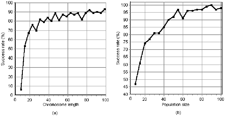
Figure 5.6: The relationship between the success rate of the MEP algorithm and (a) number of genes in a chromosome, (b) the number of individuals in population. Results are averaged over 100 runs.

Figure 5.6 shows that MEP is able to find a correct digital circuit in multiple runs. A population consisting of 90 individuals with 20 genes yields a success rate of 100% (see Figure 5.6(b)) and a population with 20 individuals with 85 genes yields a success rate of 92% (see Figure 5.6(a)).

From Figure 5.6(a) we may infer that larger MEP chromosomes are better than the shorter ones. The minimum number of gates for this circuit is 7. This number has been achieved by Miller during his numerical experiments (see [58]). A MEP chromosome implementing Miller’s digital circuit has 11 genes (the actual digital circuit + 4 input genes). From Figure 5.6(a) we can see that, for a MEP chromosome with 11 genes, only 6 correct solutions have been evolved. As the chromosome length increases the number of correct solutions evolved by also increases. If the chromosome has more than 21 genes the success rate never decreases below than 70%.

Even if the chromosome length is larger than the minimum required (11 genes) the evolved solutions usually have no more than 14 genes. This is due to the multi expression ability of MEP which acts like a provider of variable length chromosomes [64]. The length of the obtained circuits could be reduced by adding another feature to our MEP algorithm. This feature has been suggested by C. Coello in [13] and it consists of a multiobjective fitness function. The first objective is to minimize the differences between the expected output and the actual output (see formulas (5.1) and (5.2)). The second objective is to minimize the number of gates used by the digital circuit. Note that he first objective is more important than the second one. We also have to modify the algorithm. Instead of stopping the MEP algorithm when an optimal solution (regarding the first objective) is found we continue to run the program until a fixed number of generations have been elapsed. In this way we hope that also the number of gates (the second objective) will be minimized.

Two-bit adder with carry

A more complex situation is the Two Bit Adder with Carry problem [58]. The circuit implementing this problem adds 5 bits (two numbers represented using 2 bits each and a carry bit) and gives a three-bit number representing the output.

The training set consists of 32 fitness cases with 5 inputs and 3 outputs.

The relationship between the success rate and the chromosome length and the population size is analyzed for this problem.

When the relationship between the success rate and the population size is analyzed the number of genes in each MEP chromosome is set to 20 genes. When the relationship between the success rate and the population size is analyzed a population consisting of 20 MEP chromosomes is used. Gates 10 and 16 (see Table 5.3) are used in this experiment (as indicated in [58]). Other MEP parameters are given in Table 5.4.

Results are depicted in Figure 5.7.

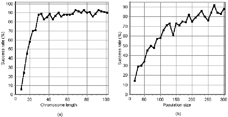
Figure 5.7: The relationship between the success rate of the MEP algorithm and (a) number of genes in a chromosome, (b) the number of individuals in population. Results are averaged over 100 runs.

Figure 5.7 shows that MEP is able solve this problem very well. When the number of genes in a MEP chromosome is larger than 30 in more than 80 cases (out of 100) MEP was able to find a perfect solution (see Figure 5.7(a)). After this value, the success rate does not increase significantly. A population with 270 individuals yields over 90 (out of 100) successful runs (see Figure 5.7(b)).

This problem is more difficult than the two-bit multiplier even if we used a smaller function set (functions 10 and 16) that the set used for the multiplier (function 6, 7 and 10).

Two-bit adder

The circuit implementing the N-Bit Adder problem adds two numbers represented using $N$ bits each and gives a ($N$ + 1)-bit number representing the output.

The training set for this problem consists of 16 fitness cases with 4 inputs and 3 outputs.

For this problem the relationship between the success rate and the chromosome length and the population size is analyzed.

When the relationship between the success rate and the population size is analyzed the number of genes in each MEP chromosome is set to 12 genes. When the relationship between the success rate and the chromosome length is analyzed a population consisting of 100 MEP chromosomes is used.

Gates 0 to 9 (see Table 5.3) are used in this experiment. Other MEP parameters are given in Table 5.8.

Table 5.8: Parameters of the MEP algorithm for evolving digital circuits.

Parameter	Value
Crossover type	Uniform
Crossover probability	0.9
Mutation	2 symbols / chromosome
Selection	Binary Tournament

For reducing the chromosome length and for preventing input redundancy we keep all terminals on the first positions of the MEP chromosomes.

Results are depicted in Figure 5.8

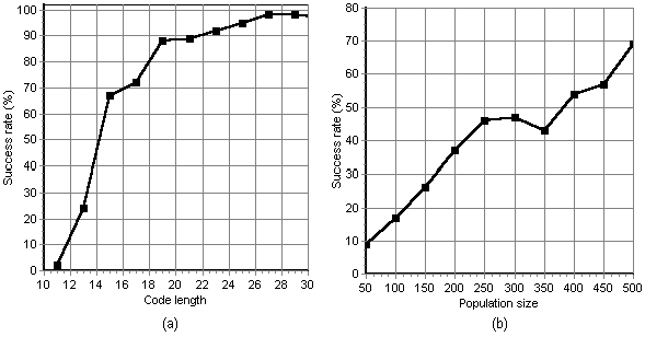
Figure 5.8: The relationship between the success rate of the MEP algorithm and (a) number of genes in chromosome, (b) the number of individuals in population. Results are averaged over 100 runs.

Figure 5.8 shows that MEP is able solve this problem very well. When the number of genes in a MEP chromosome is 27 in more than 98 cases (out of 100) MEP was able to find a perfect solution (see Figure 5.8(a)). After this value, the success rate does not increase significantly. A population with 500 individuals yields over 69 (out of 100) successful runs (see Figure 5.8(b)). The success rate for this problem may be increased by reducing the set of function symbols to an optimal set.

From Figure 5.8(a) we may infer that larger MEP chromosomes are better than the shorter ones. The minimum number of gates for this circuit is 7. A MEP chromosome implementing the optimal digital circuit has 11 genes (the actual digital circuit + 4 genes storing the inputs). From Figure 5.8(a) we can see that, for a MEP chromosome with 11 genes, only 2 correct solutions have been evolved. As the chromosome length increases the number of correct solutions evolved by also increases. If the chromosome has more than 21 genes the success rate never decreases below than 89%.

Three-bit adder

The training set for this problem consists of 64 fitness cases with 6 inputs and 4 outputs.

Due to the increased size of the training set we analyze in this section only the cumulative probability of success and the computation effort over 100 independent runs.

Gates 0 to 9 (see Table 5.3) are used in this experiment. Other MEP parameters are given in Table 5.9.

Table 5.9: Parameters of the MEP algorithm for solving the 3-Bit Adder problem.

Parameter	Value
Population size	2000
Code Length	30 genes
Crossover type	Uniform
Crossover probability	0.9
Mutation	2 symbols / chromosome
Selection	Binary Tournament

Results are depicted in Figure 5.9.

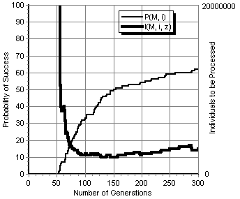
Figure 5.9: The cumulative probability of success and the number of individuals to be processed in order to obtained a solution with 99% probability. Results are averaged over 100 runs.

Figure 5.9 shows that MEP is able solve this problem very well. In 62 cases (out of 100) MEP was able to produce a perfect solution. The minimum number of individuals required to be processed in order to obtain a solution with a 99% probability is 2030000. This number was obtained at generation 145. The shortest evolved circuit for this problem contains 12 gates.

Four-bit adder: preliminary results

The training set for this problem consists of 256 fitness cases, each of them having 8 inputs and 5 outputs. Due to the increased complexity of this problem we performed only 30 independent runs using a population of 5000 individuals having 60 genes each. The number of generations was set to 1000.

In 24 (out of 30) runs MEP was able to find a perfect solution. The shortest evolved digital circuit contains 19 gates. Further numerical experiments will be focused on evolving more efficient circuits for this problem.

Two-bit multiplier

The two-bit multiplier circuit implements the binary multiplication of two $N$-bit numbers to produce a possible 2 * $N$-bit number.

The training set for this problem consists of 16 fitness cases, each of them having 4 inputs and 4 outputs.

Several experiments for evolving a circuit that implements the two-bit multiplier are performed. Since the problem has a reduced computational complexity we perform a detailed analysis by computing the relationship between the success rate and the code length and the population size.

The number of genes in each MEP chromosome is set to 14 genes when the relationship between the success rate and the population size is analyzed. When the relationship between the success rate and the chromosome length is analyzed a population consisting of 50 MEP chromosomes is used. Gates 0 to 9 (see Table 5.3) are used in this experiment. Other MEP parameters are given in Table 5.4.

Results are depicted in Figure 5.10.

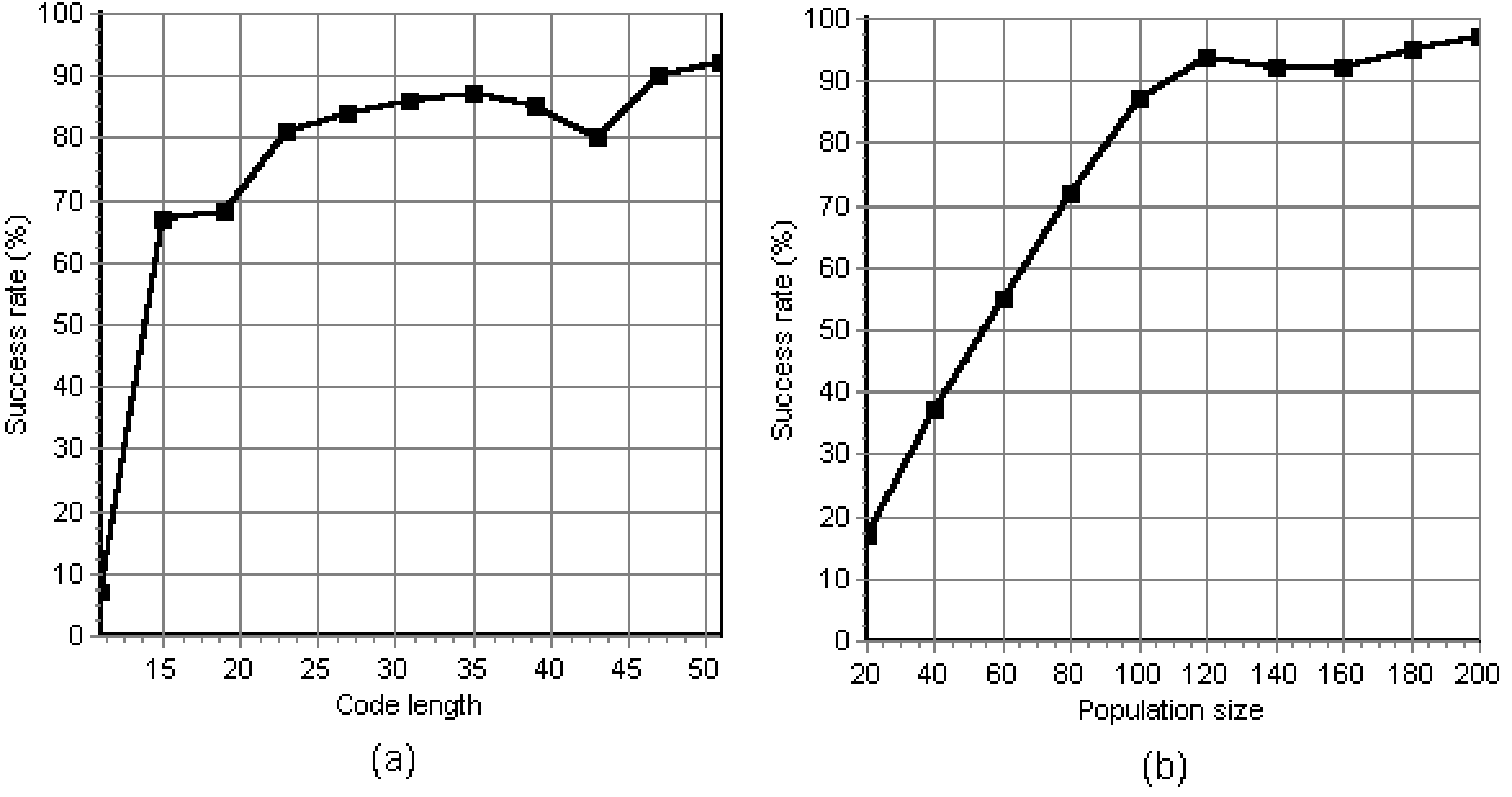
Figure 5.10: The relationship between the success rate of the MEP algorithm and (a) number of genes in a chromosome, (b) the number of individuals in population. Results are averaged over 100 runs.

Figure 5.10 shows that MEP is able to find a correct digital circuit in many runs. A population consisting of 120 individuals with 14 genes yields a success rate of 94% (see Figure 5.10(b)) and a population with 50 individuals with 47 genes yields a success rate of 90% (see Figure 5.10(a)). We can see that the success rate increase with more than 60% from MEP chromosomes with 11 genes to MEP chromosomes with 15 genes. The minimum number of gates required by this circuit is 7 and it has been obtained in most of the runs.

3-Bit multiplier

The training set for this problem consists of 64 fitness cases, each of them having 6 inputs and 6 outputs.

This problem turned out to be more difficult than the corresponding 3-Bit Adder (see section 5.3.4). Using a population of 10000 individuals each having 100 genes we have obtained only 20 perfect solutions (out of 50 independent runs). The shortest evolved digital circuit contains 35 gates. Further research will be focused on evolving more efficient circuits for this problem.

5.4 Designing digital circuits for NP-Complete problems

MEP is used for evolving digital circuits for a well-known NP-Complete [31] problem: the knapsack (subset sum) problem. Numerical results are reported in [71].

Since this problem is NP-Complete we cannot realistically expect to find a polynomial-time algorithm for it. Instead, we have to speed-up the existing techniques in order to reduce the time needed to obtain a solution. A possibility for speeding-up the algorithms for this problem is to implement them in assembly language. This could lead sometimes to improvements of over two orders of magnitude. Another possibility is to design and build a special hardware dedicated to that problem. This approach could lead to significantly improvements of the running time. Due to this reason we have chosen to design, by the means of evolution, digital circuits for several instances of the knapsack problem.

5.4.1 Evolving circuits for the knapsack problem

The knapsack problem may also be used as benchmarking problem for the evolutionary techniques which design electronic circuits. The main advantage of the knapsack problem is its scalability: increasing the number of inputs leads to more and more complicated circuits. The results show that MEP performs very well for all the considered test problems.

The knapsack problem is a well-known NP-Complete problem [31]. No polynomial-time algorithm is known for this problem.

Instead of designing a heuristic for this problem we will try to evolve digital circuits which will provide the answer for a given input.

In the experiments performed in this section the set $M$ consists of several integer numbers from the set of consecutive integers starting with 1. For instance if the base set is {1, 2, 3, 4, 5, 6, 7} then $M$ may be {2, 5, 6}. We will try to evolve a digital circuit that is able t provide the correct answer for all subsets $M$ of the base set.

The input for this problem is a sequence of bits. A value of 1 in position $k$ means that the integer number $k$ belongs to the set $M$, otherwise the number $k$ does not belong to the set $M$.

For instance consider the consecutive integer numbers starting with 1 and ending with 7. The string 0100110 encodes the set $M$ = {2, 5, 6}. The number 1, 3, 4 and 7 do not belong to $M$ since the corresponding positions are 0. The possible subsets of $M$ instance have the sum 2, 5, 6, 7, 8, 11 or 13. In our approach, the target sum is fixed and we are asking if is there a subset of given sum.

The number of training instances for this problem depends on the number of consecutive integers used as base for $M$. If we use numbers 1, 2 and 3, we have 2³ = 8 training instances. If we use number 1, 2, 3, 4, 5, 6 and 7, we have 2⁷ = 128 training instances. In this case, whichever subset $M$ of {1,…,7} will be presented to the evolved circuit we have to obtain a binary answer whether the target sum $k$ may or not be obtained from a subset of $M$.

5.4.2 Numerical experiments

In this section several numerical experiments for evolving digital circuits for the knapsack problem are performed. The general parameters of the MEP algorithm are given in Table 5.10. Since different instances of the problem being solved will have different degrees of difficulty we will use different population sizes, number of genes in a chromosome and number of generations for each instance. Particular parameters are given in Table 5.11.

Table 5.10: General parameters of the MEP algorithm for evolving digital circuits.

Parameter	Value
Crossover probability	0.9
Crossover type	Uniform
Mutations	5 / chromosome
Function set	Gates 0 to 9
Terminal set	Problem inputs
Selection	Binary Tournament

Table 5.11: Particular parameters of the MEP algorithm for different instances of the knapsack problem. In the second column the base set of numbers is given for each instance. In the third column the target sum is given.

#	Set of numbers	Sum	Number of fitness cases	Population size	Number of genes	Number of generations
1	{1…4}	5	16	20	10	51
2	{1…5}	7	32	100	30	101
3	{1…6}	10	64	500	50	101
4	{1…7}	14	128	1000	100	201

Experimental results are given in Table 5.12. We are interested in computing the number of successful runs and the number of gates in the shortest evolved circuit.

Table 5.12: Results obtained by MEP for the considered test problems. 100 independent runs have been performed for all problems.

#	Set of numbers	Sum	Successful runs	Number of gates in the shortest circuit
1	{1…4}	5	39 out of 100	3
2	{1…5}	7	31 out of 100	5
3	{1…6}	10	10 out of 100	11
4	{1…7}	14	7 out of 100	21

Table 5.12 shows that MEP successfully found at least a solution for the considered test problems. The difficulty of evolving a digital circuit for this problem increases with the number of inputs of the problem. Only 20 individuals are required to obtain 39 solutions (out of 100 runs) for the instance with 4 inputs. In return, 1000 individuals (50 times more) are required to obtain 10 perfect solutions (out of 100 independent runs) for the instance with 7 inputs. Also the size of the evolved circuits increases with the number of problem inputs. However, due to the reduced number of runs we cannot be sure that we have obtained the optimal circuits. Additional experiments are required in this respect.

Due to the NP-Completeness of the problem it is expected that the number of gates in the shortest circuit to increase exponentially with the number of inputs.

5.5 Conclusions and Further Work

In this section, Multi Expression Programming has been used for evolving digital circuits. It has been shown the way in which multiple digital circuits may be encoded in the same chromosome and the way in which MEP chromosomes are read only once for computing their quality. There was no human input about how the circuits should be designed, just a measurement of the degree to which a given circuit achieves the desired response.

Several numerical experiments for evolving digital circuits have been performed. The circuits evolved during the numerical experiments are for the 2 and 3-bit Multiplier, the 2, 3 and 4-bit Adder problems, even-parity, NP-complete problems and multiplexers.

These problems are well-known benchmark instances used for assessing the performance of the algorithms evolving digital circuits.

Further numerical experiments with Multi Expression Programming will be focused on evolving digital circuits for other interesting problems.

Chapter 6 MEP for Evolving Algorithms and Game Strategies

6.1 Discovering game strategies

In this section we investigate the application of MEP technique for discovering game strategies. This chapter is entirely original and it is based on the papers [64, 70, 76].

Koza [42] suggested that GP can be applied to discover game strategy. The game-playing strategy may be viewed as a computer program that takes the information about the game as its input and produces a move as output.

The available information may be an explicit history of previous moves or an implicit history of previous moves in the form of a current state of game (e.g. the position of each piece on the chess board) [42].

Tic-tac-toe (TTT, or naughts and crosses) is a game with simple rules, but complex enough to illustrate the ability of MEP to discover game strategy.

6.1.1 TTT game description

In Tic-Tac-Toe there are two players and a 3 $\times$ 3 grid. Initially the grid is empty. Each player moves in turn by placing a marker in an open square. By convention, the first player’s marker is ”X” and the second player’s marker is ”0”.

The player that put three markers of his type (”X” for the first player and ”0” for the second player) in a row is declared the winner.

The game is over when one of the players wins or all squares are marked and no player wins. In the second case, the game ends with draw (none of the players win). Enumerating the game tree shows that the second player can obtain at least a draw.

A well-known evolutionary algorithm that evolves game strategy has been proposed in [12]. This algorithm will be reviewed in the next section.

6.1.2 Chellapilla’s approach of TTT

In [12] Evolutionary Programming has been used in order to obtain a good strategy (that never loses) for the Tic-Tac-Toe game. A strategy is encoded in a neural network. A population of strategies encoded by neural networks is evolved.

Each network receives a board pattern as input and yields a move as output. The aim is to store in a neural network the function that gives the quality of a configuration. When a configuration is presented to the network, the network output (supplies) the next move.

Each neural network has an input layer with 9 nodes, an output layer with 9 nodes, and a hidden layer with a variable number of nodes.

Fogel’s algorithm starts with a random population of 50 neural networks. For each network the number of nodes from the hidden layer is randomly chosen with a uniform distribution over integers 1…10. The initial weighted connection strengths and bias terms are randomly distributed according to a uniform distribution ranging over [-0.5, 0.5].

From each parent a single offspring is obtained by mutation. Mutation operator affects the hidden layer structure, weight connections and bias terms.

Each strategy encoded in a neural network was played 32 times against a heuristic rule base procedure.

The payoff function has several values corresponding to winning, loosing and draw.

The best individuals from a generation are retained to form the next generation.

The process is evolved for 800 generations. According to [12], the best obtained neural network is able to play to win or draw with a perfect play strategy.

6.1.3 MEP approach of TTT

In this section we illustrate the use of MEP to discover an unbeatable play strategy for Tic-Tac-Toe.

We are searching for a mathematical function $F$ that gives the quality of each game configuration. Using this function the best configurations that can be reached in one move from the current configuration, is selected. Therefore function $F$ supplies the move to be performed for each game configuration.

Function $F$ evaluating each game configuration is represented as a MEP chromosome. The best expression encoded by a chromosome is chosen to be the game strategy of that chromosome.

Without any loose of generality we may allow MEP strategy to be the first player in each game.

All expressions in the chromosome are considered in the fitness assignment process. Each expression is evaluated using an ”all-possibilities” procedure. This procedure executes all moves that are possible for the second player. The fitness of an expression $E$ is the number of games that the strategy encoded by the expression $E$ loses. Obviously the fitness has to be minimized.

Let us denote by

$P$ = ($p_{0}$, $p_{1}$…$p_{8})$

a game configuration.

Each $p_{k}$ describes the states ”X”, ”0” or an empty square. In our experiments the set {5, -5, 2} has been used for representing the symbols ”X”, ”0” and the empty square.

The game board has been linearized by scanning board squares from up to down and from left to right. Thus the squares in the first line have indices 0, 1 and 2, etc. (see Figure 6.1).

Figure 6.1: Game board linearized representation.

Algorithm parameters are given in Table 6.1.

Table 6.1: Algorithm parameters for TTT game.

Parameter	Value
Population size	50
Chromosome length	50 genes
Mutation probability	0.05
Crossover type	Two-point-crossover
Selection	Binary tournament
Elitism size	1
Terminal set	$T$ = {$p_{0}$, $p_{1}$,…, $p_{8}$}
Function set	$F$ = {+, -, *, /}

The MEP algorithm is able to evolve a perfect, non-loosing, game strategy in 11 generations. This process requires less than 10 seconds when an Intel Pentium 3 processor at 1GHz is used.

In Figure 6.2, the fitness of the best individual in the best run and average fitness of the best individuals over all runs are depicted.

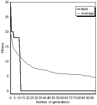
Figure 6.2: Fitness of the best individual in the best runs and the average fitness of the best individuals over all runs. The results are taken over 30 runs.

Figure 6.2 shows that an individual representing a non-loosing strategy appears in the population at generation 14.

Some functions evolved by the MEP algorithm are given below:

$F_{1}(P)$ = (($p_{4}-p_{5}$-($p_{6}+p_{5}))$*$p_{8}+p_{4}$*$p_{3})$*($p_{4}-p_{7})$,

$F_{2}(P)$ = $p_{2}$-($p_{8}$*$p_{7}-p_{4})-p_{7}$-($p_{2}$*$p_{5})$,

$F_{3}(P)$ = ($p_{4}$*$p_{1}+p_{2})$*$p_{7}$-($p_{1}-p_{2}+p_{7}$*$p_{5})$-($p_{8}$-($p_{3}$*$p_{5}))$.

These functions do not force the win when it is possible, but they never lose. This is a consequence of fitness assignment process. However, the proposed technique can also generate a function that forces the win whenever it is possible.

It is not easy to compare this result with the result obtained by Chellapilla and Fogel [12] as the experiment conditions were not the same. In [12] evolved strategies play against a heuristic procedure, but here MEP formulas play against an all-moves procedure. Population size was the same (50 individuals). Individual sizes are difficult to be compared. All MEP individual have the same size: 148 symbols. Neural network’s sizes used in [12] are variable since the hidden layer contains a variable number of nodes. If the number of nodes in the hidden layer is 9, then the size of the neural network (biases + connection weights) is 9 * 9 + 9 * 9 * 9 + 9 * 9 = 324.

MEP approach seems to be faster as MEP was able to discover a non-losing strategy in no more than 17 generations. As noted in [12] neural network approach requires 800 generations.

A TTT heuristic vs. MEP approach

A good heuristic for Tic-Tac-Toe is described in what follows:

S1. If a winning move is available make that move, else

S2. If a winning move is available for the opponent, move to block it, else

S3. If a move of the opponent that leads to two winning ways is available, block that move, else

S4. If the board center is available, move in the board center,

S5. If one ore more corners of the table are available, move in one of them, else

S6. Move randomly in an available square.

This heuristic performs well on most of the game positions. However, by applying one of the formulas evolved by the MEP algorithm some benefits are obtained:

• easy implementation in programming languages,

• MEP evolved formula is a faster algorithm than the previously shown heuristic.

Applying MEP for generating complex game strategies

Using the all-possibilities technique (a backtracking procedure that plays all the moves for the second player) allows us to compute the absolute quality of a game position.

For complex games a different fitness assignment technique is needed since the moves for the second player can not be simulated by an all-possibilities procedure (as the number of moves that needs to be simulated is too large).

One fitness assignment possibility is to use a heuristic procedure that acts as the second player. But there are several difficulties related to this approach. If the heuristic is very good it is possible that none of evolved strategy could ever beat the heuristic. If the heuristic procedure plays as a novice then many evolved strategy could beat the heuristic from the earlier stages of the search process. In the last case fitness is not correctly assigned to population members and thus we can not perform a correct selection.

A good heuristic must play on several levels of complexity. At the beginning of the search process the heuristic procedure must play at easier levels. As the search process advances, the level of difficulty of the heuristic procedure must increases.

However, for complex games such a procedure is difficult to implement.

Another possibility is to search for a game strategy using a coevolutionary algorithm [12]. This approach seems to offer the most spectacular results. In this case, MEP population must develop intelligent behavior based only on internal competition.

6.2 Evolving winning strategies for Nim-like games

In this section, we propose an evolutionary approach for computing the winning strategy for Nim-like games. The proposed approach is is entirely original and it is reported in the paper [76].

6.2.1 Introduction

Nim is one of the older two-person games known today. Whereas the standard approaches for determining winning strategies for Nim are based on the Grundy-Sprague theory [8, 14], this problem can be solved using other techniques. For instance, the first winning strategy for this game was proposed in 1901 by L.C. Bouton from the Harvard University. The Bouton’s solution is based on computing the xor sum of the numbers of objects in each heap. In other words Bouton computed a relation between the current state of the game and the player which has a winning strategy if it is his/her turn to move.

In this section, we propose an evolutionary approach for computing the winning strategy for Nim-like games. The proposed approach is based on Multi Expression Programming. The idea is to find a mathematical relation (an expression) between the current game state and the winner of the game (assuming that both players do not make wrong moves). The searched expression should contain some mathematical operators (such as +, -, *, div, mod, and, or, not, xor) and some operands (encoding the current game state).

It is widely known [8, 30] that a winning strategy is based on separation of the game’s states in two types of positions: $P$-positions (advantage to the previous player) and $N$-positions (advantage to the next player). Our aim is to find a formula that is able to detect whether a given game position belongs to $P$-positions or to $N$-positions. Our formula has to return 0 if the given position is a $P$-position and a nonzero value otherwise. That could be easily assimilated to a symbolic regression [42] or a classification task. It is well-known that machine learning techniques (such as Neural Networks or Evolutionary Algorithms [34] are very suitable for solving this kind of problems. However, the proposed approach is different from the classical approaches mainly because the $P$ and $N$-positions are usually difficult to be identified for a new game. Instead we propose an approach that checks $P$ and $N$-position during the traversing of the game tree.

This theory can be easily extended for other games that share several properties with the Nim game (i.e. games for which the winning strategy is based on $P$ and $N$-positions).

The problem of finding $N$ and $P$-positions could be also viewed as a classification task with two classes. However, we do not use this approach because in this case it is required to know the class ($P$ or $N)$ for each game position.

The results presented in this section enter in the class of human-competitive results produced by an artificial machine. According to [42, 44] a result produced by an artificial machine is considered intelligent if it is equal or better than a result that was accepted as a new scientific result at the time when it was published in a peer-reviewed scientific. A list with other human-competitive results produced by the Genetic Programming can be found in [44].

6.2.2 Basics on Nim game

Nim is one of the oldest and most engaging of all two-person mathematical games known today [8, 14]. The name and the complete theory of the game were invented by the professor Charles Leonard Bouton from Harvard University about 100 years ago.

Players take turns removing objects (counters, pebbles, coins, pieces of paper) from heaps (piles, rows, boxes), but only from one heap at a time. In the normal convention the player who removes the last object wins.

The usual practice in impartial games is to call a hot position ($N$-position - advantage to the next player, i.e. the one who is about to make a move) and a cold one ($P$-position - advantage to the previous player, i.e. the one who has just made a move).

In 1930, R. P. Sprague and P. M. Grundy developed a theory of impartial games in which Nim played a most important role. According to the Sprague-Grundy theory every position in an impartial game can be assigned a Grundy number which makes it equivalent to a Nim heap of that size. The Grundy number of a position is variously known as its Nim-heap or nimber for short [8, 14].

A P-position for the Nim game is given by the equation:

$x_{1}$ xor $x_{2}$ xor …xor $x_{n}$ = 0,

where $n$ is the number of heaps, $x_{i}$ is the number of objects in the $i^{th}$ heap and xor acts as the modulo 2 operator.

A variant of the Nim game, also analyzed in this section, is the one in which players may remove no more than $k$ objects from a heap. In this variant a $P$-position is characterized by the equation:

($x_{1}$ mod $k)$ xor ($x_{2}$ mod $k)$ xor …xor ($x_{n}$ mod $k)$ = 0,

where the equation parameters have been previously explained.

Due to the way of computing $P$-position we shall call this game NimModK.

6.2.3 Fitness assignment process

The procedure used for computing the quality of a chromosome is described in this section.

Even if this problem could be easily handled as a classification problem (based on a set of fitness cases), we do not use this approach since for the new games it is difficult to find which the $P$-positions and $N$-positions are. Instead we employ an approach based on the traversing the game tree. Each nod in this tree is a game configuration (state).

There are three theorems that run the winning strategy for the Nim game [8]:

• Any move applied to a $P$-position turns the game into a $N$-position.

• There is at least one move that turns the game from a $N$-position into a $P$-position.

• The final position (when the game is over) is a $P$-position.

The value of the expression encoded into a MEP chromosome is computed for each game state. If the obtained value is 0, the corresponding game state is considered as being a $P$-position, otherwise the configuration is considered as being a $N$-position.

The fitness of a chromosome is equal to the number of violations of the above described rule that arises in a game tree. Thus, if the current formula (chromosome) indicates that the game state encoded into a node of the game tree is a $P$-position and (the same current formula indicates that) all the game states encoded in the offspring nodes are also $P$-positions means that we have a violation of the rule $b)$.

Since we do not want to have violations of the previously described rule, our chromosome must have the fitness equal to zero. This means that the fitness has to be minimized.

For a better understanding of the fitness assignment process we provide an example where we shall compute by hand the fitness of a chromosome.

Consider the game state (2,1), and a MEP chromosome encoding the expression $E=a_{1}-a_{2}$*$a_{1}$. The game tree of the Nim game is given in Figure 6.3.

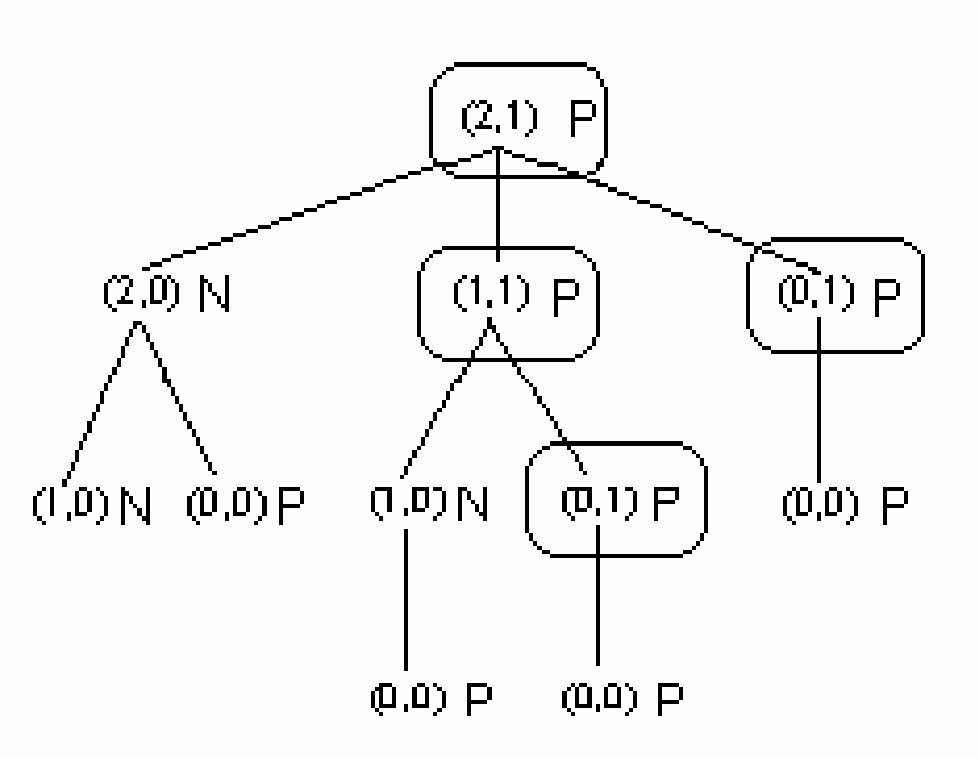
Figure 6.3: The game tree for a Nim game that starts with the configuration (2, 1). At the right side of each game configuration is printed the configuration’ state ($P$-position or $N$-position) as computed by the formula $E=a_{1}-a_{1}$*$a_{2}$. The configurations that violate one of the three rules described above are encircled.

Figure 6.3 shows that the fitness of a MEP chromosome encoding the formula $E=a_{1}-a_{2}$*$a_{1}$ is four (there are four violations of the winning strategy rules).

6.2.4 Numerical experiments

Several numerical for evolving winning strategies for Nim-like games are performed in this section.

The purpose of these experiments is to evolve a formula capable to distinguish between a $N$-position and a $P$-position for the Nim game. We shall analyze the relationships between the success rate and the population size, the chromosome length and the number of generations used during the search process.

In all the experiments it is considered the following configuration for the Nim game: (4, 4, 4, 4). This configuration has been chosen in order to have a small computational time. However, this configuration has proved to be enough for evolving a winning strategy.

The total number of game configurations is 70 (which can be obtained either by counting nodes in the game tree or by using the formula of combinations with repetitions). Two permutations of the same configuration are not considered different.

Remark
The success rate is computed by using the formula:

$$\mbox{Success}\,\mbox{rate}=\frac{\mbox{the number of successful }\,\mbox{runs}}{\mbox{the total number of runs}}.$$

Experiment 1

In the first experiment the relationship between the population size and the success rate is analyzed. MEP algorithm parameters are given in Table 6.2.

Table 6.2: MEP algorithm parameters for Experiment 1.

Parameter	Value
Chromosome length	15 genes
Number of generations	100
Crossover probability	0.9
Mutations	2 mutations / chromosome
Selection strategy	binary tournament
Terminal set	$T_{Nim}$ = {$n$, $a_{1}$, $a_{2}$, …, $a_{n}$}.
Function set	$F$= {+, -, *, div, mod, and, not, xor, or}

The results of this experiment are depicted in Figure 6.4.

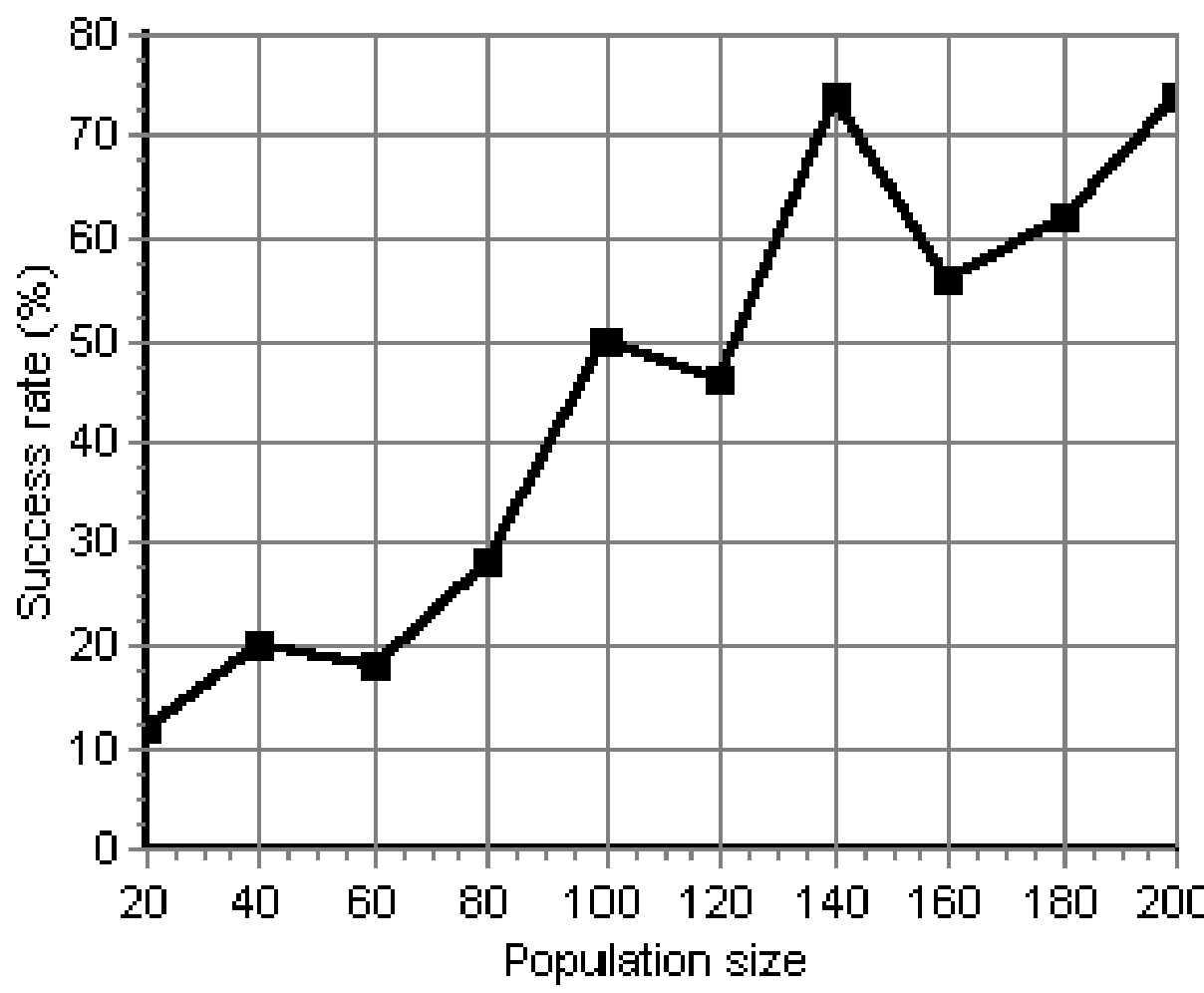
Figure 6.4: The relationship between the population size and the rate of success. The results are averaged over 50 runs. The population size varies between 20 and 200.

Figure 6.4 shows that the success rate increases as the population size increases. The highest value - 37 successful runs (out of 50) - is obtained with a population containing 140 individuals. Even a population with 20 individuals is able to yield 6 successful runs (out of 50).

Experiment 2

In the second experiment the relationship between the number of generations and the success rate is analyzed. MEP algorithm parameters are given in Table 6.3.

Table 6.3: MEP algorithm parameters for Experiment 2.

Parameter	Value
Chromosome length	15 genes
Population Size	100 individuals
Crossover probability	0.9
Mutations	2 mutations / chromosome
Selection strategy	binary tournament
Terminal set	$T_{Nim}$ = {$n$, $a_{1}$, $a_{2}$, …, $a_{n}$}.
Function set	$F$= {+, -, *, div, mod, and, not, xor, or}

The results of this experiment are depicted in Figure 6.5.

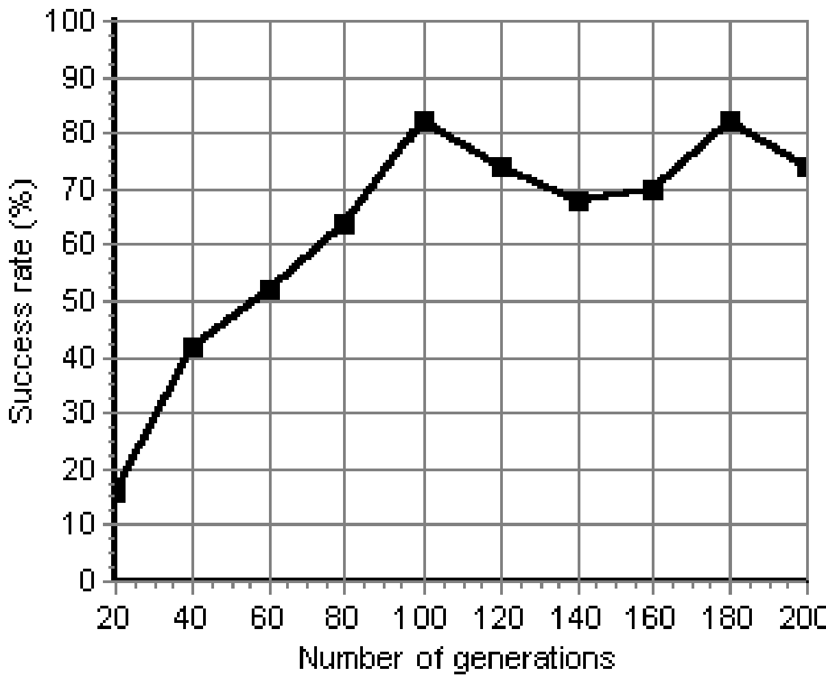
Figure 6.5: The relationship between the number of generations and the rate of success. The results are averaged over 50 runs. The number of generations varies between 20 and 200.

Figure 6.5 shows that MEP is able to find a winning strategy for the Nim game in most of the runs. In 41 runs (out of 50) a perfect solutions was obtained after 100 generations. 9 successful runs were obtained when the algorithm is run for 20 generations.

Experiment 3

In the third experiment the relationship between the chromosome length and the success rate is analyzed. MEP algorithm parameters are given in Table 6.4.

Table 6.4: MEP algorithm parameters for Experiment 3.

Parameter	Value
Number Of Generations	50
Population Size	100 individuals
Crossover probability	0.9
Mutations	2 mutations / chromosome
Selection strategy	binary tournament
Terminal set	$T_{Nim}$ = {$n$, $a_{1}$, $a_{2}$, …, $a_{n}$}.
Function set	$F$= {+, -, *, div, mod, and, not, xor, or}

The results of this experiment are depicted in Figure 6.6.

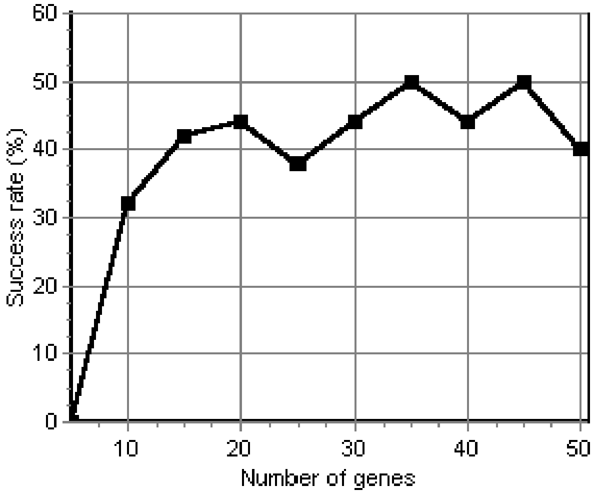
Figure 6.6: The relationship between the chromosome length and the success rate. The results are averaged over 50 runs. The chromosome length varies between 5 and 50.

Figure 6.6 shows that the optimal number of genes of a MEP chromosome is 35. With this value 25 runs (out of 50) were successful.

It is interesting to note that the formulas evolved by MEP are sometimes different from the classical $a_{1}$ xor $a_{2}$ xor $a_{3}$ xor $a_{4}$. For instance a correct formula evolved by MEP is:

$F=a_{1}$ xor $a_{2}$ xor $a_{3}\quad-$ $a_{4}$.

This formula is also correct due to the properties of the xor operator.

Experiment 4

In this experiment a formula for the NimModK game is evolved. The initial configuration was the same (4, 4, 4, 4) and $k$ was set to 2. The parameters for the MEP algorithm are given in Table 6.5.

Table 6.5: MEP algorithm parameters for Experiment 4.

Parameter	Value
Chromosome length	35 genes
Number of generations	100
Population size	1000 individuals
Crossover probability	0.9
Mutations	2 mutations / chromosome
Selection strategy	binary tournament
Terminal set	$T_{NimModK}$ = {$n$, $k$, $a_{1}$, $a_{2}$, …, $a_{n}$}.
Function set	$F$= {+, -, *, div, mod, and, not, xor, or}

This problem turned out to be more difficult than the previous one. In only 3 runs (out of 50) MEP was able to find a perfect formula (i.e. a formula that has the fitness equal to 0).

6.3 Evolving heuristics for NP-Complete problems

MEP technique is used for discovering TSP heuristics for graphs satisfying triangle inequality (TI graphs). This option was chosen due to the existence of a big number of real-world applications implying TI graphs (e.g. plains, trains and vehicles routes). MEP technique is used to learn a path function $f$ that is used for evaluating the reachable nodes. This function serves as a heuristic for detecting the optimum path.

This section is entire original and it is based on the paper [70].

6.3.1 MEP for TSP

In the proposed approach the TSP path starts with a randomly selected node of the graph. Each node reachable from the current node in one step is evaluated using the function (computer program) $f$ evolved by MEP algorithm. The best node is added to the already detected path. The algorithm stops when the path contains all graph nodes.

MEP learning process for TSP has a remarkable quality: the evolved (learned) heuristic works very well for data sets much larger than the training set. For MEP training stage graphs having 3 to 50 nodes are considered. Evolved MEP function was tested and performs well for graphs having maximum 1000 nodes.

Evolved function $f$ is compared with some well known heuristics. Numerical experiments emphasize that (for considered examples) MEP function outperforms dedicated heuristics.

6.3.2 TSP problem with triangle inequality

TSP problem for TI graphs (i.e. satisfying triangle inequality) is stated as follows.

Consider a set $C$ = {$c_{0}$, $c_{1}$,…, $c_{N\mbox{--}1}$} of cities, and a distance $d(c_{i}$, $c_{j})\quad\in$ Z⁺ for each pair $c_{i}$, $c_{j}\quad\in\quad C,d(c_{i}$, $c_{j})=d(c_{j}$, $c_{i})$, and for each three cities $c_{i}$, $c_{j}$, $c_{k}\quad\in\quad C$, $d(c_{i}$, $c_{j})\quad\leq$ $d(c_{i}$, $c_{k})+d(c_{k}$, $c_{j})$. The tour $<$c_π(0), c_π(1), …, c${}_{\pi(N\mbox{--}1)}>$ of all cities in $C$ having minimum length is needed [1, 31]

TSP problem with triangle inequality is an NP-complete problem [31]. No polynomial time algorithm for solving TSP problem is known.

Several heuristics for solving TSP problem have been proposed. The most important are Nearest Neighbor and the Minimum Spanning Tree [15, 31].

In this section we address the problem of discovering heuristics that can solve TSP rather than solving a particular instance of the problem.

MEP technique is used for evolving a path function $f$ that gives a way to choose graph vertices in order to obtain a Hamiltonian cycle. The fitness is assigned to a function $f$ in the current population by applying $f$ on several randomly chosen graphs (training set) and evaluating the results.

Evolved path function may be used for solving particular instances of TSP. For each problem the graph nodes are evaluated using the path function $f$ and are added one by one to the already build path.

The algorithm for TSP using evolved path function $f$ may be described as follows:

$S_{1}$. Let $c_{\pi(0)}=c_{0}$ {the path starts with the node c₀}

$S_{2}$. $k$ = 1;

$S_{3}$. while $k<N$ – 1 do

$S_{4}$.          Using function $f$ select $c_{\pi(k+1)}$ – the next node of the path

$S_{5}$.          Add $c_{\pi(k+1)}$ to the already built path.

$S_{6}$.          $k=k$ + 1;

$S_{7}$. endwhile

$S_{4}$ is the key step of this algorithm. The procedure that selects the next node of the path in an optimal way uses the function $f$ evolved by the MEP technique as described in the next sections.

6.3.3 Terminals and functions for evolving heuristic function f

Path function $f$ has to use (as input) some information about already build path and some information about unvisited nodes. We consider a special terminal set which is independent with respect to the number of graph nodes.

Let us denote by $y_{1}$ the last visited node (current node). We have to select the next node to be added to the path. In this respect all unvisited nodes are considered. Let us denote by $y_{2}$ the next node to be visited.

For evolving path function $f$ we consider a set $T$ of terminals involving the following elements:

d_y₁_y₂ – distance between the graph nodes $y_{1}$ and $y_{2}$,

min_g_y₁ (min_g_y${}_{2})$ – the minimum distance from the nodes $y_{1}$ ($y_{2})$ to unvisited nodes,

sum_g_y₁ (sum_g_y${}_{2})$ – the sum of all distances between nodes $y_{1}$ ($y_{2})$ and unvisited nodes,

prod_g_y₁ (prod_g_y${}_{2})$ – the product of all distances between nodes $y_{1}$ ($y_{2})$ and unvisited nodes,

max_g_y₁ (max_g_y${}_{2})$ – the maximum distance from the nodes $y_{1}$ ($y_{2})$ to unvisited nodes,

length – the length of the already built path.

The set $T$ of terminals (function variables) is thus:

$T$ = {d_y₁_y₂, min_g_y₁, min_g_y₂, max_g_y₁, max_g_y₂, sum_g_y₁, sum_g_y₂, prod_g_y₁, prod_g_y₂, length}.

Let us remark that members of $T$ are not actual terminals (in the standard acceptation). For this reason we may call members of $T$ as instantiated (or intermediate) nonterminals.

Set $T$ of terminals is chosen in such way to be independent of the number of graph nodes. This choice confers flexibility and robustness to the evolved heuristic.

For evolving a MEP function for TSP problem we may consider the following set of function symbols: $F$ = {+, -, /, *, cos, sin, min, max}.

The node $y_{2}$ that generates the lowest output of evolved function $f$ is chosen to be the next node of the path. Ties are solved arbitrarily. For instance we may consider the node with the lowest index is selected.

Example

Consider the MEP linear structure:

1: $d$_$y_{1}$_$y_{2}$

2: min_g_y₁

3: + 1, 2

4: sum_g_y₂

5: * 2, 4

This MEP individual encodes the path functions $f_{1}$, $f_{2}$, $f_{3}$, $f_{4}$, $f_{5}$ given by:

$f_{1}=d$_$y_{1}$_$y_{2}$,

$f_{2}$ = min_g_y₁,

$f_{3}=d$_$y_{1}$_$y_{2}$ + min_g_y₁,

$f_{4}$ = sum_g_y₂,

$f_{5}$ = min_g_y₁* sum_g_y₂.

6.3.4 Fitness assignment

In order to obtain a good heuristic we have to train the path function $f$ using several graphs. The training graphs are randomly generated at the beginning of the search process and remain unchanged during the search process. To avoid overfitting (see [86]), another set of randomly generated graphs (validation set) is considered. After each generation the quality of the best-so-far individual is calculated using the validation set in order to check its generalization ability during training. At the end of the search process, the function with the highest quality is supplied as the program output.

The fitness (quality) of a detected path function $f$ is defined as the sum of the TSP path length of graphs in the training set. Thus the fitness is to be minimized.

6.3.5 A numerical experiment

In this experiment we evolve a heuristic for solving TSP problem.

Let us denote by $G_{k}$ the set of class of TI graphs having maximum $k$ nodes.

MEP algorithm considers the class $G_{50}$ (i.e. graphs having 3 to 50 nodes) for training and the class $G_{100}$ for validation. Evolved path function was tested for graphs in the class $G_{1000}$ (i.e. graphs having maxim 1000 nodes). MEP algorithm parameters are given in Table 6.6.

Table 6.6: MEP algorithm parameters for evolving a heuristic for TSP with triangle inequality

Parameter	Value
Population size	300
Number of generations	100
Chromosome length	40 genes
Mutation probability	0.1
Crossover type	One-Crossover-Point
Crossover probability	0.9
Training set size	30
Maximum number of nodes in training set	50
Validation set size	20
Maximum number of nodes in validation set	100

The evolution of the best individual fitness and the average fitness of the best individuals over 30 runs are depicted in Table 6.7.

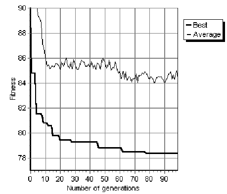
Figure 6.7: The fitness evolution of the best individual in the best run and the average fitness of the best individuals over 30 runs.

A path function evolved by the MEP algorithm is:

$f$ = (sum_g($y2))$ * (d_y₁_y₂ - (max(d_y₁_y₂, max_g($y_{1}))$) + d_y₁_y${}_{2})$.

Heuristic function $f$ that is evolved by MEP technique is directly used for building the optimum path. The corresponding learning process has a remarkable quality: the evolved (learned) heuristic works very well on data sets significantly larger than the training set. In our example the training set $G_{50}$ is significantly smaller than the set $G_{1000}$ used for testing.

6.3.6 Assessing the performance of the evolved MEP heuristic

In this section the performance of evolved MEP heuristic, NN and MST are compared. In the first experiment we compare the considered algorithms on some randomly generated graphs. In the second experiment the heuristics are compared against several difficult problems in TSPLIB [87].

Experiment 1

In this experiment we provide a direct comparison of the evolved MEP heuristic, NN and MST. The considered heuristics are tested for randomly generated graphs satisfying triangle inequality.

Evolved heuristic was tested for different graphs from the classes $G_{200}$, $G_{500}$ and $G_{1000}$. For each graph class 1000 graphs satisfying triangle inequality have been randomly generated. These graphs have been considered for experiments with evolved MEP heuristic, NN and MST.

Performance of evolved MEP heuristic, NN and MST are depicted in Table 6.7.

Table 6.7: Evolved MEP heuristic vs. NN, MST. For each graph class we present the number of graphs for which evolved MEP heuristic generates a cycle shorter than the cycle obtained by the algorithm MST and NN.

Graphs types	MST	NN
$G_{200}$	953	800
$G_{500}$	974	906
$G_{1000}$	990	948

Results obtained emphasizes that evolved MEP heuristic outperforms NN and MST algorithms on random graphs.

Experiment 2

To obtain a stronger evidence of the results above we test the performance of the considered heuristics against some difficult problems in TSPLIB. The results are presented in Table 6.8.

Table 6.8: The performance of evolved MEP heuristic, NN and MST on some problems in TSPLIB. Length is the length of the TSP path obtained with one of the considered heuristics. Error is calculated as (Length - Shortest_Length)/ Shortest_Length * 100. Each node of the graph has been considered as the first node of the path

Problem	MEP		NN		MST
	Length	Error (%)	Length	Error (%)	Length	Error (%)
a280	2858.86	10.85	3084.22	19.58976	3475.23	34.75
att48	37188.2	10.93	39236.9	17.04227	43955.8	31.11
berlin52	7672.1	1.72	8182.19	8.488332	10403.9	37.94
bier127	134945	14.08	127954	8.177068	152747	29.13
ch130	6558.03	7.33	7198.74	17.81899	8276.51	35.45
ch150	7104.03	8.82	7078.44	8.431985	9142.99	40.05
d198	17780.7	12.67	17575.1	11.37579	17957.6	13.79
d493	43071.3	23.05	41167	17.61328	41846.6	19.55
d657	56965.6	16.46	60398.7	23.48442	63044.2	28.89
eil101	685.013	8.9	753.044	19.72083	846.116	34.51
eil51	441.969	3.74	505.298	18.61455	605.049	42.03
eil76	564.179	4.86	612.656	13.87658	739.229	37.4
fl417	13933.8	17.47	13828.2	16.58545	16113.2	35.85
gil262	2659.17	11.82	2799.49	17.72456	3340.84	40.48
kroA150	28376.3	6.98	31482	18.6925	38754.8	46.11
kroA200	32040.3	9.09	34547.7	17.63722	40204.1	36.89
kroB100	24801	12.01	25883	16.90077	28803.5	30.09
kroB200	33267.4	13.01	35592.4	20.91042	40619.9	37.98
lin105	15133.2	5.24	16939.4	17.80652	18855.6	31.13
lin318	46203.4	9.93	49215.6	17.09915	60964.8	45.05
pcb442	56948.3	12.15	57856.3	13.9397	73580.1	44.9
pr226	84937.8	5.68	92905.1	15.59818	111998	39.35
pr264	55827.1	13.61	54124.5	10.15468	65486.5	33.27
rat195	2473.49	6.47	2560.62	10.22901	2979.64	28.26
rat575	7573.6	11.82	7914.2	16.84925	9423.4	39.13
rat783	9982.96	13.36	10836.6	23.05928	11990.5	36.16
rd400	16973.3	11.07	18303.3	19.77816	20962	37.17
ts225	136069	7.44	140485	10.92994	187246	47.85
u574	43095.6	16.77	44605.1	20.86465	50066	35.66
u724	46545.7	11.06	50731.4	21.04844	60098.9	43.39

From Table 6.8 we can see that evolved MEP heuristic performs better than NN and MST on most of the considered problems. Only for five problems (bier127, ch150, d198, d493, fl417) NN performs better than evolved MEP heuristic. MST does not perform better than evolved MEP heuristic for no problem. The highest error obtained by the evolved MEP heuristic is 23.05 (the problem d493) while the highest error obtained by NN is 23.45 (the problem rd400). The lowest error obtained with MEP is 1.72 (problem berlin52) while the lowest error obtained by NN is 8.17 (problem bier127). The mean of errors for all considered problems is 10.61 (for evolved MEP heuristic) 16.33 (for NN heuristic) and 35.77 (for MST heuristic).

6.4 Conclusions and further work

Three approaches have been proposed in this section:

• an evolutionary approach for the Nim game. The underlying evolutionary technique is Multi Expression Programming - a very fast and efficient Genetic Programming variant. Numerical experiments have shown that MEP is able to discover a winning strategy in most of the runs.

  The proposed method can be easily applied for games whose winning strategy is based on $P$ and $N$-positions. The idea is to read the game tree and to count the number of configurations that violates the rules of the winning strategy.

• an evolutionary approach for the Tic-Tac-Toe game. Evolved strategy is very fast. About 400.000 games/second can be played without loss.

• an evolutionary approach for evolving heuristics for the TSP. Numerical experiments have shown that the evolved heuristic performs better than the NN and MST heuristics.

6.4.1 Applying MEP for generating complex game strategies

Using the all-possibilities technique (a backtracking procedure that plays all the moves for the second player) allows us to compute the absolute quality of a game position. For complex games a different fitness assignment technique is needed since the moves for the second player can not be simulated by an all-possibilities procedure (as the number of moves that needs to be simulated is too large). One fitness assignment possibility is to use a heuristic procedure that acts as the second player. But there are several difficulties related to this approach. If the heuristic is very good it is possible that none of evolved strategy could ever beat the heuristic. If the heuristic procedure plays as a novice then many evolved strategy could beat the heuristic from the earlier stages of the search process. In the last case fitness is not correctly assigned to population members and thus we can not perform a correct selection. A good heuristic must play on several levels of complexity. At the beginning of the search process the heuristic procedure must play at easier levels. As the search process advances, the level of difficulty of the heuristic procedure must increases. However, for complex games such a procedure is difficult to implement. Another possibility is to search for a game strategy using a coevolutionary algorithm. This approach seems to offer the most spectacular results. In this case, MEP population must develop intelligent behavior based only on internal competition.

Chapter 7 Infix Form Genetic Programming

A new GP variant called Infix Form Genetic Programming (IFGP) is described. IFGP individuals are arrays of integer values encoding mathematical expressions in infix form. IFGP is used for solving real-world classification problems.

The chapter is entirely original and it is based on the paper [67].

7.1 Introduction

Classification is the task of assigning inputs to a number of discrete categories or classes [38]. Examples include classifying a handwritten letter as one from A-Z, classifying a speech pattern to the corresponding word, etc.

Machine learning techniques have been extensively used for solving classification problems. In particular Artificial Neural Networks (ANNs) [38, 86] have been originally designed for classifying a set of points in two distinct classes. Genetic Programming (GP) techniques [42] have also been used for classification purposes. For instance, LGP [9] has been used for solving several classification problems in PROBEN1. The conclusion was that LGP is able to solve the classification problems with the same error rate as a neural network.

Infix Form Genetic Programming (IFGP), chromosomes are strings encoding complex mathematical expressions using infix form. An interesting feature of IFGP is its ability of storing multiple solutions of a problem in a chromosome.

In what follows IFGP is described and used for solving several real-world classification problems taken from PROBEN1 [86].

7.2 Prerequisite

We denote by $F$ the set of function symbols (or operators) that may appear in a mathematical expression. $F$ usually contains the binary operators {+, $-$, *, /}. Number_of_Operators denotes the number of elements in $F$. A correct mathematical expression also contains some terminal symbols. The set of terminal symbols is denoted by $T$. The number of terminal symbols is denoted by Number_of_Variables.

The symbols that may appear in a mathematical expression encoded by the IFGP are from the set $T\quad\cup$ $F\quad\cup$ {’(’, ’)’}. The total number of symbols that may appear in a valid mathematical expression is denoted by Number_of_Symbols.

By $C_{i}$ we denote the value on the $i^{th}$ gene in a IFGP chromosome and by $G_{i}$ the symbol in the $i^{th}$ position in the mathematical expression encoded into an IFGP chromosome.

7.3 Individual representation

In this section we describe how IFGP individuals are represented and how they are decoded in order to obtain a valid mathematical expression.

Each IFGP individual is a fixed size string of genes. Each gene is an integer number in the interval [0 .. Number_Of_Symbols - 1]. An IFGP individual can be transformed into a functional mathematical expression by replacing each gene with an effective symbol (a variable, an operator or a parenthesis).

Example

If we use the set of functions symbols $F$ = {+, *, -, /}, and the set of terminals $T$ = {$a$, $b$}, the following chromosome

C = 7, 3, 2, 2, 5

is a valid chromosome in IFGP system.

7.4 Decoding IFGP individuals

We will begin to decode this chromosome into a valid mathematical expression. In the first position (in a valid mathematical expression) we may have either a variable, or an open parenthesis. That means that we have Number_Of_Variables + 1 possibilities to choose a correct symbol on the first position. We put these possibilities in order: the first possibility is to choose the variable $x_{1}$, the second possibility is to choose the variable $x_{2}$ …the last possibility is to choose the closed parenthesis ’)’. The actual value is given by the value of the first gene of the chromosome. Because the number stored in a chromosome gene may be larger than the number of possible correct symbols for the first position we take only the value of the first gene modulo number of possibilities for the first gene.

Generally, when we compute the symbol stored in the $i^{th}$ position in expression we have to compute first how many symbols may be placed in that position. The number of possible symbols that may be placed in the current position depends on the symbol placed in the previous position. Thus:

• if the previous position contains a variable ($x_{i})$, then for the current position we may have either an operator or a closed parenthesis. The closed parenthesis is considered only if the number of open parentheses so far is larger than the number of closed parentheses so far.

• if the previous position contains an operator, then for the current position we may have either a variable or an open parenthesis.

• if the previous position contains an open parenthesis, then for the current position we may have either a variable or another open parenthesis.

• if the previous position contains a closed parenthesis, then for the current position we may have either an operator or another closed parenthesis. The closed parenthesis is considered only if the number of open parentheses so far is larger than the number of closed parentheses.

Once we have computed the number of possibilities for the current position it is easy to determine the symbol that will be placed in that position: first we take the value of the corresponding gene modulo the number of possibilities for that position. Let $p$ be that value

($p=C_{i}$ mod Number_Of_Possibilities).

The $p^{th}$ symbol from the permitted symbols for the current is placed in the current position in the mathematical expression. (Symbols that may appear into a mathematical expression are ordered arbitrarily. For instance we may use the following order: $x_{1}$, $x_{2}$, …, +, -, *, /, ’(’, ’)’. )

All chromosome genes are translated but the last one. The last gene is used by the correction mechanism (see below).

The obtained expression usually is syntactically correct. However, in some situations the obtained expression needs to be repaired. There are two cases when the expression needs to be corrected:

The last symbol is an operator (+, -, *, /) or an open parenthesis. In that case a terminal symbol (a variable) is added to the end of the expression. The added symbol is given by the last gene of the chromosome.

The number of open parentheses is greater than the number of closed parentheses. In that case several closed parentheses are automatically added to the end in order to obtain a syntactically correct expression.

Remark
If the correction mechanism is not used, the last gene of the chromosome will not be used.

Example

Consider the chromosome

$C$ = 7, 3, 2, 0, 5, 2

and the set of terminal and function symbols previously defined

$T$ = {$a$, $b$},

$F$ = {+, -, *, /}.

For the first position we have 3 possible symbols ($a$, $b$ and ‘(‘). Thus, the symbol in the position $C_{0}$ mod 3 = 1 in the array of possible symbols is placed in the current position in expression. The chosen symbol is $b$, because the index of the first symbol is considered to be 0.

For the second position we have 4 possibilities (+, -, *, /). The possibility of placing a closed parenthesis is ignored since the difference between the number of open parentheses and the number of closed parentheses is zero. Thus, the symbol ’/’ is placed in position 2.

For the third position we have 3 possibilities ($a$, $b$ and ’(’). The symbol placed on that position is an open parenthesis ’(’.

In the fourth position we have 3 possibilities again ($a$, $b$ and ’(’). The symbol placed on that position is the variable $a$.

For the last position we have 5 possibilities (+, -, *, /) and the closed parenthesis ’)’. We choose the symbol on the position 5 mod 5 = 0 in the array of possible symbols. Thus the symbol ‘+’ is placed in that position.

The obtained expression is $E=b$ / ($a$+.

It can be seen that the expression $E$ it is not syntactically correct. For repairing it we add a terminal symbol to the end and then we add a closed parenthesis. Now we have obtained a correct expression:

$E=b$ / ($a+a)$.

The expression tree of $E$ is depicted in Figure 7.1.

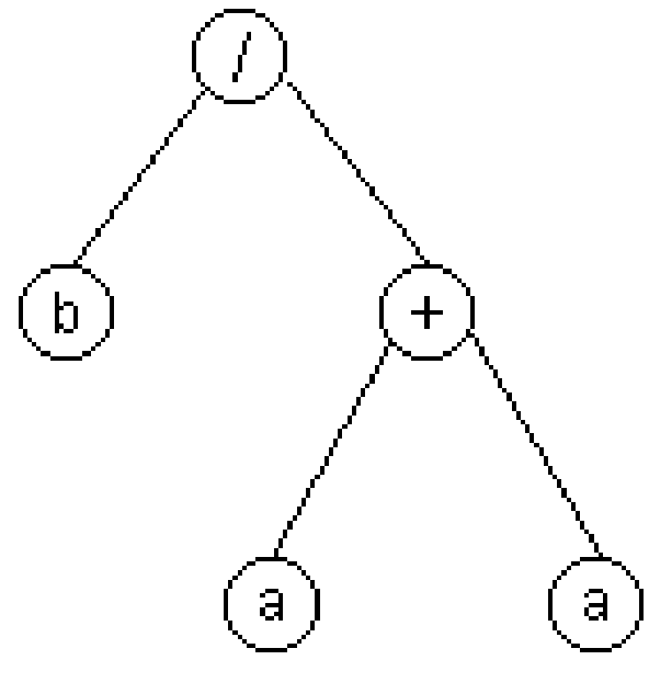
Figure 7.1: The expression tree of $E=b$ / ($a+a)$.

7.5 Using constants within the IFGP model

An important issue when designing a new GP technique is the way in which the constants are embaded into the proposed model.

Fixed or ephemeral random constants have been extensively tested within GP systems [42]. The interval over which the constants are initially generated is usually problem-dependent. For a good functionality of the program a priori knowledge about the required constants is usually needed.

By contrast, IFGP involves a problem-independent system of constants.

It is known that each real number may be written as a sum of powers of 2.

Within the IFGP model each constant is a power of 2. The total number of constants is also problem-independent. For instance, if we want to solve problems using double precision constants, we need 127 constants:

2^-63, 2^-62,…, 2^-1, 2⁰, 2¹,…, 2⁶³.

Particular instances of the classification problems may require fewer constants. As can be seen in section 7.4 a good solution for some classification problems can be obtained without using constants. However, if we do not know what kind of constants are required by the problems being solved it is better the use the double precision system of constants (as described above).

Within the IFGP chromosome each constant is represented by its exponent. For instance the constant 2¹⁷ is stored as the number 17, the constant 2^-4 is stored as the number -4 and the constant 1 = 2⁰ is stored as the number 0. These constants will act as terminal symbols. Thus the extended set of terminal symbols is

$T$ = {$x_{1}$, $x_{2}$,…, -63, -62, .., -1, 0, 1, …, 62, 63}.

7.6 Fitness assignment process

In this section we describe how IFGP may be efficiently used for solving classification problems.

A GP chromosome usually stores a single solution of a problem and the fitness is normally computed using a set of fitness cases.

Instead of encoding a single solution, an IFGP individual is allowed to store multiple solutions of a problem. The fitness of each solution is computed in a conventional manner and the solution having the best fitness is chosen to represent the chromosome.

In the IFGP representation each sub-tree (sub-expression) is considered as a potential solution of a problem.

Example

The previously obtained expression (see section 7.4) contains 4 distinct solutions (sub-expressions):

$E_{1}=a$,

$E_{2}=b$,

$E_{3}=a+a$,

$E_{4}=b$ / ($a+a)$.

Now we will explain how the fitness of a (sub)expression is computed.

Each class has associated a numerical value: the first class has the value 0, the second class has the value 1 and the $m^{th}$ class has associated the numerical value $m-$1. Any other system of distinct numbers may be used. We denote by $o_{k}$ the number associated to the $k^{th}$ class.

The value $v_{j}(E_{i})$ of each expression $E_{i}$ (in an IFGP) chromosome for each row (example) $j$ in the training set is computed. Then, each row in the training set will be classified to the nearest class (the class $k$ for which the difference $|v_{j}(E_{i})-o_{k}|$ is minimal). The fitness of a (sub)expression is equal to the number of incorrectly classified examples in the training set. The fitness of an IFGP chromosome will be equal to the fitness of the best expression encoded in that chromosome.

Remarks

• Since the set of numbers associated with the problem classes was arbitrarily chosen it is expected that different systems of number to generate different solutions.

• When solving symbolic regression or classification problems IFGP chromosomes need to be traversed twice for computing the fitness. That means that the complexity of the IFGP decoding process it is not higher than the complexity of other methods that store a single solution in a chromosome.

7.7 Search operators

Search operators used within the IFGP model are recombination and mutation. These operators are similar to the genetic operators used in conjunction with binary encoding [19].

7.7.1 Crossover

By recombination two parents exchange genetic material in order to obtain two offspring. In our numerical experiments only two-point recombination is used.

7.7.2 Mutation

Mutation operator is applied with a fixed mutation probability ($p_{m})$. By mutation a randomly generated value over the interval [0, Number_of_Symbols-1] is assigned to the target gene.

7.8 Handling exceptions within IFGP

Exceptions are special situations that interrupt the normal flow of expression evaluation (program execution). An example of exception is division by zero which is raised when the divisor is equal to zero.

GP techniques usually use a protected exception handling mechanism [42]. For instance if a division by zero exception is encountered, a predefined value (for instance 1 or the numerator) is returned. This kind of handling mechanism is specific for Linear GP [9], standard GP [42] and GE [82].

IFGP uses a new and specific mechanism for handling exceptions. When an exception is encountered (which is always generated by a gene containing a function symbol), the entire (sub) tree which has generated the exception is mutated (changed) into a terminal symbol. Exception handling is performed during the fitness assignment process.

7.9 IFGP algorithm

A steady-state [95] variant of IFGP is employed in this section. The algorithm starts with a randomly chosen population of individuals. The following stpng are repeated until a termination condition is reached. Two parents are chosen at each step using binary tournament selection [19]. The selected individuals are recombined with a fixed crossover probability $p_{c}$. By recombining two parents, two offspring are obtained. The offspring are mutated and the best of them replaces the worst individual in the current population (only if the offspring is better than the worst individual in population).

The algorithm returns as its answer the best expression evolved for a fixed number of generations.

7.10 Solving classification problems using IFGP

IFGP technique is applied for solving difficult learning problems. Real-world data sets are considered for the training process.

7.10.1 Data sets

Numerical experiments performed in this section are based on several benchmark problems taken from PROBEN1 [86]. These datasets were created based on the datasets from the UCI Machine Learning Repository [103].

Used problems are briefly described in what follows.

Cancer

Diagnosis of breast cancer. Try to classify a tumor as either benignant or malignant based on cell descriptions gathered by microscopic examination.

Diabetes

Diagnosis diabetes of Pima Indians. Based on personal data and the results of medical examinations try to decide whether a Pima Indian individual is diabetes positive or not.

Heartc

Predicts heart disease. Decides whether at least one of four major vessels is reduced in diameter by more than 50%. The binary decision is made based on personal data such as age, sex, smoking habits, subjective patient pain descriptions and results of various medical examinations such as blood pressure and electro cardiogram results.

This data set was originally created by Robert Detrano from V.A. Medical Center Long Beach and Cleveland Clinic Foundation.

Horse

Predicts the fate of a horse that has colic. The results of a veterinary examination of a horse having colic are used to predict whether the horse will survive will die or should be euthanized.

The number of inputs, of classes and of available examples, for each test problem, are summarized in Table 7.1.

Table 7.1: Summarized attributes of several classification problems from PROBEN1.

Problem	Number of inputs	Number of classes	Number of examples
cancer	9	2	699
diabetes	8	2	768
heartc	35	2	303
horse	58	3	364

7.10.2 Numerical experiments

The results of several numerical experiments with ANNs, LGP and IFGP are presented in this section.

Each data set is divided in three sub-sets (training set -50%, validation set - 25 %, and test set - 25%) (see [86]).

The test set performance is computed for that chromosome which had minim validation error during the search process. This method, called early stopping, is a good way to avoid overfitting [86] of the population individuals to the particular training examples used. In that case the generalization performance will be reduced.

In [9] Linear GP was used to solve several classification problems from PROBEN1. The parameters used by Linear GP are given in Table 7.2.

Table 7.2: Linear GP parameters used for solving classification tasks from PROBEN1

Parameter	Value
Population size	5000
Number of demes	10
Migration rate	0.05
Classification error weight in fitness	1.0
Maximum number of generations	250
Crossover probability	0.9
Mutation probability	0.9
Maximum mutation step size for constants	$\pm 5$
Maximum program size	256 instructions
Initial maximum program size	25 instructions
Function set	{+, -, *, /, sin, exp, if $>$, if $\leq$}
Terminal set	{0,..,256} $\cup$ {input variables}

IFGP algorithm parameters are given in Table 7.3.

Table 7.3: IFGP algorithm parameters for solving classification problems from PROBEN1.

Parameter	Value
Population Size	250
Chromosome length	30
Number of generations	250
Crossover probability	0.9
Crossover type	Two-point Crossover
Mutation	2 mutations per chromosome
Number of Constants	41 {2-20, …, 20, 220}
Function set	{+, -, *, /, sin, exp}
Terminal set	{input variables} $\cup$ The set of constants.

The results of the numerical experiments are presented in Table 7.4.

Table 7.4: Classification error rates of IFGP, LGP and ANN for some date sets from PROBEN1. LGP results are taken from [9]. ANNs results are taken from [86]. The cases where IFGP is better than LGP have been written on a grey background. The cases where IFGP is better than ANNs have been bolded and italicized. Results are averaged over 30 runs

Problem	IFGP–test set			LGP–test set			NN–test set
	best	mean	stddev	best	mean	stddev	mean	stddev
cancer1	1.14	2.45	0.69	0.57	2.18	0.59	1.38	0.49
cancer2	4.59	6.16	0.45	4.02	5.72	0.66	4.77	0.94
cancer3	3.44	4.92	1.23	3.45	4.93	0.65	3.70	0.52
diabetes1	22.39	25.64	1.61	21.35	23.96	1.42	24.10	1.91
diabetes2	25.52	28.92	1.71	25.00	27.85	1.49	26.42	2.26
diabetes3	21.35	25.31	2.20	19.27	23.09	1.27	22.59	2.23
heart1	16.00	23.06	3.72	18.67	21.12	2.02	20.82	1.47
heart2	1.33	4.40	2.35	1.33	7.31	3.31	5.13	1.63
heart3	12.00	13.64	2.34	10.67	13.98	2.03	15.40	3.20
horse1	23.07	31.11	2.68	23.08	30.55	2.24	29.19	2.62
horse2	30.76	35.05	2.33	31.87	36.12	1.95	35.86	2.46
horse3	30.76	35.01	2.82	31.87	35.44	1.77	34.16	2.32

Table 7.4 shows that IFGP is able to obtain similar performances as those obtained by LGP even if the population size and the chromosome length used by IFGP are smaller than those used by LGP. When compared to ANNs we can see that IFGP is better only in 3 cases (out of 12).

We are also interested in analysing the relationship between the classification error and the number of constants used by the IFGP chromosomes. For this purpose we will use a small population made up of only 50 individuals. Note that this is two magnitude orders smaller than those used by LGP. Other IFGP parameters are given in Table 7.3. Experimental results are given in Table 7.5.

Table 7.5: Classification error rates of IFGP (on the test set) using different number of constants. The cases where IFGP is better than LGP have been written on a grey background. The cases where IFGP is better than ANNs have been bolded and italicized. Results are averaged over 30 runs.

Problem	IFGP–41 constants			IFGP–0 constants			IFGP–81 constants
	best	mean	stddev	best	mean	stddev	best	mean	stddev
cancer1	1.14	2.45	0.60	1.14	3.18	1.06	1.14	2.41	0.77
cancer2	4.02	6.16	0.91	4.02	6.14	0.81	4.59	6.24	0.99
cancer3	3.44	5.17	1.10	2.87	5.07	1.50	2.87	5.15	1.07
diabetes1	22.39	25.74	2.19	21.87	26.04	1.76	21.87	25.34	2.08
diabetes2	26.04	29.91	1.65	25.00	29.21	2.21	25.52	29.82	1.30
diabetes3	21.87	25.34	1.76	19.79	24.79	1.91	22.91	25.88	3.60
heart1	17.33	24.44	3.76	18.67	23.28	3.33	18.66	25.28	3.64
heart2	1.33	6.97	4.07	1.33	4.97	3.16	1.33	7.06	4.60
heart3	12.00	14.00	2.51	10.67	15.42	3.40	9.33	15.11	4.25
horse1	26.37	32.16	3.12	25.27	30.69	2.49	27.47	31.57	1.91
horse2	30.76	35.64	2.37	30.76	35.49	2.81	31.86	35.71	2.23
horse3	28.57	34.13	3.14	28.57	35.67	3.90	28.57	34.90	3.53

Table 7.5 shows that the best results are obtained when the constants are not used in our IFGP system. For 8 (out of 12) cases the best result obtained by IFGP outperform the best result obtained by LGP. That does not mean that the constants are useless in our model and for the considered test problems. An explanation for this behaviour can be found if we take a look at the parameters used by IFGP. The population size (of only 50 individuals) and the chromosome length (of only 30 genes) could not be enough to obtain a perfect convergence knowing that some problems have many parameters (input variables). For instance the horse problem has 58 attributes and a chromosome of only 30 genes could not be enough to evolve a complex expression that contains sufficient problem’s variables and some of the considered constants. It is expected that longer chromosomes will increase the performances of the IFGP technique.

7.11 Conclusion and further work

An evolutionary technique, Infix Form Genetic Programming (IFGP) has been described in this chapter. The IFGP technique has been used for solving several classification problems. Numerical experiments show that the error rates obtained by using IFGP are similar and sometimes even better than those obtained by Linear Genetic Programming.

Further numerical experiments will try to analyse the relationship between the parameters of the IFGP algorithm and the classification error for the considered test problems.

Chapter 8 Multi Solution Linear Genetic Programming

A new Linear Genetic Programming [9] variant called Multi-Solution Linear Genetic Programming (MS-LGP) is described. Each MS-LGP chromosome encodes multiple solutions of the problem being solved. The best of these solutions is used for fitness assignment purposes.

This chapter is entirely original and it is based on the papers [74, 78].

8.1 MS-LGP representation and fitness assignment process

MS-LGP enrichs LGP structure in two ways:

• Each destination variable is allowed to represent the output of the program. In the standard LGP only one variable is chosen to provide the output.

• The program output is checked after each instruction in chromosome. Note that within the standard LGP the output is checked after the execution of all instructions in a chromosome.

After each instruction, the value stored in the destination variable is considered as a potential solution of the problem. The best value stored in one of the destination variables is considered for fitness assignment purposes.

Example

Consider the chromosome $C$ given below:

void LGP(double r[8])

{

$r$[5] = $r$[3] * $r$[2];

$r$[3] = $r$[1] + 6;

$r$[0] = $r$[4] * $r$[7];

$r$[6] = $r$[4] – $r$[1];

$r$[1] = $r$[6] * 7;

$r$[0] = $r$[0] + $r$[4];

$r$[2] = $r$[3] / $r$[4];

}

Instead of encoding the output of the problem in a single variable (as in SS-LGP) we allow that each of the destination variables ($r$[5], $r$[3], $r$[0], r[6], $r$[1] or $r$[2]) to store the program output. The best output stored in these variables will provide the fitness of the chromosome.

For instance, if we want to solve symbolic regression problems, the fitness of each destination variable $r$[$i$] may be computed using the formula:

$$f(r[i])=\sum\limits_{k=1}^{n}{\left|{o_{k,i}-w_{k}}\right|},$$

where $o_{k,i}$ is the result obtained in variable $r$[$i$] for the fitness case $k$, $w_{k}$ is the targeted result for the fitness case $k$ and $n$ is the number of fitness cases. For this problem the fitness needs to be minimized.

The fitness of an individual is set to be equal to the lowest fitness of the destination variables encoded in the chromosome:

$$f(C)=\mathop{\min}\limits_{i}f(r[i]).$$

Thus, we have a Multi-Solution program at two levels:

• First level is given by the possibility that each variable to represent the output of the program.

• Second level is given by the possibility of checking for the output at each instruction in the chromosome.

Our choice was mainly motivated by the No Free Lunch Theorems for Search [100, 101]. There is neither practical nor theoretical evidence that one of the variables employed by the LGP is better than the others. More than that, Wolpert and McReady [100] proved that we cannot use the search algorithm’s behavior so far for a particular test function to predict its future behavior on that function.

The Multi-Solution ability has been tested within other evolutionary model such as Multi Expression Programming [64] or Infix Form Genetic Programming [67]. For these methods it has been shown [64] that encoding multiple solutions in a single chromosome leads to significant improvements.

8.2 Numerical experiments

In this section several experiments with SS-LGP and MS-LGP are performed. For this purpose we use several well-known symbolic regression problems. The problems used for assessing the performance of the compared algorithms are:

$f_{1}(x)=x^{4}+x^{3}+x^{2}+x$.

$f_{2}(x)=x^{6}$ – 2$x^{4}+x^{2}$.

$f_{3}(x)$ = sin($x^{4}+x^{2})$.

$f_{4}(x)$ = sin($x^{4})$ + sin($x^{2})$.

For each function 20 fitness cases have been randomly generated with a uniform distribution over the [0, 1] interval.

The general parameters of the LGP algorithms are given in Table 8.1. The same settings are used for Multi Solution LGP and for Single-Solution LGP.

Table 8.1: The parameters of the LGP algorithm for symbolic regression problems.

Parameter	Value
Number of generations	51
Crossover probability	0.9
Crossover type	Uniform
Mutations	2 / chromosome
Function set	$F$ = {+, -, *, /, sin}
Terminal set	Problem inputs + 4 supplementary registers
Constants	Not used
Selection	Binary Tournament
Algorithm	Steady State

For all problems the relationship between the success rate and the chromosome length and the population size is analyzed. The success rate is computed as the number of successful runs over the total number of runs.

Experiment 1

In this experiment the relationship between the success rate and the chromosome length is analyzed. For this experiment the population size was set to 50 individuals. Other parameters of the LGP algorithms are given in Table 8.1. Results are depicted in Figure 8.1.

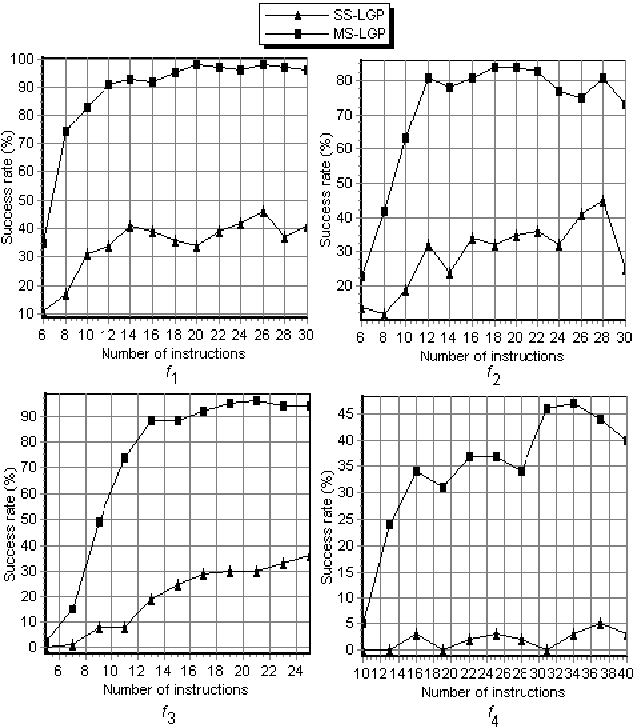
Figure 8.1: The relationship between the success rate and the number of instructions in a chromosome. Results are averaged over 100 runs.

Figure 8.1 shows that Multi-Solution LGP significantly outperforms Single-Solution LGP for all the considered test problems and for all the considered parameter setting. More than that, large chromosomes are better for MS-LGP than short chromosomes. This is due to the multi-solution ability: increasing the chromosome length leads to more solutions encoded in the same individual.

The easiest problem is $f_{1}$. MS-LGP success rate for this problem is over 90% when the number of instructions in a chromosome is larger than 12. The most difficult problem is $f_{4}$. For this problem and with the parameters given in Table 8.1, the success rate of the MS-LGP algorithm never increases over 47%. However, these results are very good compared to those obtained by SS-LGP (the success rate never increases over 5%).

Experiment 2

In this experiment the relationship between the success rate and the population size is analyzed. For this experiment the number of instructions in a LGP chromosome was set to 12. Other parameters for the LGP algorithms are given in Table 8.1. Results are depicted in Figure 8.2.

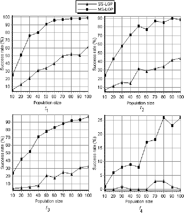
Figure 8.2: The relationship between the population size and the success rate. Population size varies between 10 and 100. Results are averaged over 100 runs.

Figure 8.2 also shows that Multi-Solution LGP performs better than Single-Solution LGP. Problem $f_{1}$ is the easiest one and problem $f_{4}$ is the most difficult one.

8.3 Conclusions and further work

The ability of encoding multiple solutions in a single chromosome has been analyzed in this chapter for Linear Genetic Programming. It has been shown how to efficiently decode the considered chromosomes by traversing them only once.

Numerical experiments have shown that Multi-Solution LGP significantly improves the evolutionary search for all the considered test problems. There are several reasons for which Multi Solution Programming performs better than Single Solution Programming:

• MS-LGP chromosomes act like variable-length chromosomes even if they are stored as fixed-length chromosomes. The variable-length chromosomes are better than fixed-length chromosomes because they can easily store expressions of various complexities,

• MS-LGP algorithms perform more function evaluations than their SS-LGP counterparts. However the complexity of decoding individuals is the same for both MS-LGP and SS-LGP techniques.

The multi-solution ability will be investigated within other evolutionary models.

Chapter 9 Evolving Evolutionary Algorithms

Two new models for evolving Evolutionary Algorithms are described in this chapter. The models are based on Multi Expression Programming and Linear Genetic Programming. Several Evolutionary Algorithms for function optimization and Traveling Salesman Problem are evolved using the proposed models.

This chapter is entirely original and it is based on the papers [63, 65].

9.1 Introduction

Evolutionary Algorithms (EAs) [39, 34] are nonconventional tools for solving difficult real-world problems. They were developed under the pressure generated by the inability of classical (mathematical) methods to solve some complex real-world problems. Many of these unsolved problems are (or could be turned into) optimization problems. Solving an optimization problem means finding of solutions that maximize or minimize a criteria function [19, 39, 34].

Many EAs were proposed for dealing with optimization problems. Many solution representations and search operators were proposed and tested within a wide range of evolutionary models. There are several natural questions that are to be answered in all of these evolutionary models:

What is the optimal population size?

What is the optimal individual representation?

What are the optimal probabilities for applying specific genetic operators?

What is the optimal number of generations before halting the evolution?

A breakthrough arose in 1995 when Wolpert and McReady unveiled their work on the No Free Lunch (NFL) theorems [100, 101]. The NFL theorems state that all of the black-box algorithms perform equally well over the entire set of optimization problems. A black-box algorithm does not take into account any information about the problem or the particular instance being solved.

The magnitudes of the NFL results stroke all of the efforts for developing a universal black-box optimization algorithm able to solve best all the optimization problems.

In their attempt to solve problems, men delegated computers to develop algorithms able to perform certain tasks. The most prominent effort in this direction is Genetic Programming (GP) [42]. Instead of evolving solutions for a particular problem instance, GP is mainly intended for discovering computer programs able to solve particular classes of problems. (This statement is only partially true, since the discovery of computer programs may be also viewed as a technique for solving a particular problem instance. The following could be an example of a problem: ”Find a computer program that calculates the sum of the elements of an array of integers.”)

There are many such approaches so far in the GP literature [42, 43, 44]. The evolving of deterministic computer programs able to solve specific problems requires a lot of effort.

Instead of evolving deterministic computer programs we evolve a full-featured evolutionary algorithm (i.e. the output of the main program will be an EA able to perform a given task). Proposed approach works with EAs at two levels:

• The first (macro) level consists of a steady-state EA [95] which uses a fixed population size, a fixed mutation probability, a fixed crossover probability etc.

• The second (micro) level consists of the solution encoded in a chromosome from the GA on the first level.

We propose two evolutionary models similar to Multi Expression Programming (MEP) [64] and Linear Genetic Programming [9]. These models are very suitable for evolving computer programs that may be easily translated into an imperative language (like C or Pascal).

9.2 Evolving evolutionary algorithms using Multi Expression Programming

In this section, Multi Expression Programming is used for evolving Evolutionary Algorithms.

9.2.1 Evolutionary model

In order to use MEP for evolving EAs we have to define a set of terminal symbols and a set of function symbols. When we define these sets we have to keep in mind that the value stored by a terminal symbol is independent of other symbols in the chromosome and a function symbol changes the solution stored in another gene.

An EA usually involves 4 types of genetic operators:

• Initialize - randomly initializes a solution,

• Select - selects the best solution among several already existing solutions

• Crossover - recombines two already existing solutions,

• Mutate - varies an already existing solution.

These operators act as symbols that may appear into an MEP chromosome. The only operator that generates a solution independent of the already existing solutions is the Initialize operator. This operator will constitute the terminal set. The other operators will be considered function symbols. Thus, we have:

$T$ = {Initialize},

$F$ = {Select, Crossover, Mutate}.

A MEP chromosome $C$, storing an evolutionary algorithm is:

1: Initialize                {Randomly generates a solution.}
2: Initialize                {Randomly generates another solution.}
3: Mutate 1               {Mutates the solution stored on position 1}
4: Select 1, 3            {Selects the best solution from those}
                                 {stored on positions 1 and 3}
5: Crossover 2, 4       {Recombines the solutions on positions 2 and 4}
6: Mutate 4                {Mutates the solution stored on position 4}
7: Mutate 5                {Mutates the solution stored on position 5}
8: Crossover 2, 6       {Recombines the solutions on positions 2 and 6}

This MEP chromosome encodes multiple evolutionary algorithms. Each EA is obtained by reading the chromosome bottom up, starting with the current gene and following the links provided by the function pointers. Thus we deal with EAs at two different levels: a micro level representing the evolutionary algorithm encoded in a MEP chromosome and a macro level GA, which evolves MEP individuals. The number of genetic operators (initializations, crossovers, mutations, selections) is not fixed and it may vary between 1 and the MEP chromosome length. These values are automatically discovered by the evolution. The macro level GA execution is bound by the known rules for GAs (see [34]).

For instance, the chromosome defined above encodes 8 EAs. They are given in Table 9.1.

Table 9.1: Evolutionary Algorithms encoded in the MEP chromosome $C$.

EA1	EA2
$i_{1}$=Initialize	$i_{1}$=Initialize
EA3	EA4
$i_{1}$=Initialize $i_{2}$=Mutate ($i_{1})$	$i_{1}$=Initialize $i_{2}$=Mutate ($i_{1})$ $i_{3}$=Select ($i_{1}$, $i_{2})$
EA5	EA6
$i_{1}$=Initialize $i_{2}$=Initialize $i_{3}$=Mutate ($i_{1})$ $i_{4}$=Select ($i_{1}$, $i_{3})$ $i_{5}$=Crossover ($i_{2}$, $i_{4})$	$i_{1}$=Initialize $i_{2}$=Mutate ($i_{1})$ $i_{3}$=Select ($i_{1}$, $i_{2})$ $i_{4}$=Mutate ($i_{3})$
EA7	EA8
$i_{1}$=Initialize $i_{2}$=Initialize $i_{3}$=Mutate ($i_{1})$ $i_{4}$=Select ($i_{1}$, $i_{3})$ $i_{5}$=Crossover ($i_{2}$, $i_{4})$ $i_{6}$ =Mutate ($i_{5})$	$i_{1}$=Initialize $i_{2}$=Initialize $i_{3}$=Mutate ($i_{1})$ $i_{4}$=Select ($i_{1}$, $i_{3})$ $i_{5}$=Mutate ($i_{4})$ $i_{6}$=Crossover ($i_{2}$, $i_{5})$

Remarks

• In our model the Crossover operator always generates a single offspring from two parents. The crossover operators generating two offspring may also be designed to fit our evolutionary model.

• The Select operator acts as a binary tournament selection. The best out of two individuals is always accepted as the selection result.

• The Initialize, Crossover and Mutate operators are problem dependent.

9.2.2 Fitness assignment

We have to compute the quality of each EA encoded in the chromosome in order to establish the fitness of a MEP individual. For this purpose each EA encoded in a MEP chromosome is run on the particular problem being solved.

Roughly speaking the fitness of a MEP individual is equal to the fitness of the best solution generated by one of the evolutionary algorithms encoded in that MEP chromosome. But, since the EAs encoded in a MEP chromosome use pseudo-random numbers it is likely that successive runs of the same EA generate completely different solutions. This stability problem is handled in the following manner: each EA encoded in a MEP chromosome is executed (run) more times and the fitness of a MEP chromosome is the average of the fitness of the best EA encoded in that chromosome over all runs. In all of the experiments performed in this section each EA encoded into a MEP chromosome was run 200 times.

9.2.3 Numerical experiments

In this section, we evolve an EA for function optimization. For training purposes we use the Griewangk’s function [102].

Griewangk’s test function is defined by the equation 9.1.

$$f(x)=\frac{1}{4000}\sum_{i=1}^{n}x_{i}^{2}-\prod_{i=1}^{n}cos\left(\frac{x_{i}}{\sqrt{i}}\right)+1.$$ (9.1)

The domain of definition is $[-500,500]^{n}$. We use $n=5$ in this study. The optimal solution is $x_{0}$ = (0,…,0) and $f(x_{0})=0$. Griewangk’s test function has many widespread local minima which are regularly distributed.

An important issue concerns the representation of the solutions evolved by the EAs encoded in an MEP chromosome and the specific genetic operators used for this purpose. The solutions evolved by the EAs encoded in MEP chromosomes are represented by using real values [34] (i.e. a chromosome of the second level EA is an array of real values). By initialization, a random point within the definition domain is generated. The convex crossover with $\alpha=\frac{1}{2}$ and the Gaussian mutation with $\sigma=0.5$ are used.

Experiment 1

In this experiment we are interested in seeing the way in which the quality of the best evolved EA improves as the search process advances. MEP algorithm parameters are given in Table 9.2.

The results of this experiment are depicted in Figure 9.1.

Table 9.2: The parameters of the MEP algorithm for Experiment 1.

Parameter	Value
Population size	100
Code Length	3000 genes
Number of generations	100
Crossover probability	0.7
Crossover type	Uniform Crossover
Mutation	5 mutations per chromosome
Terminal set	$F$ = {Initialize}
Function set	$F$ = {Select, Crossover, Mutate}

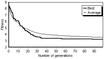
Figure 9.1: The fitness of the best individual in the best run and the average (over 10 runs) of the fitness of the best individual over all runs.

Figure 9.1 clearly shows the effectiveness of our approach. The MEP technique is able to evolve an EA for solving optimization problems. The quality of the best evolved EA is 8.5 at generation 0. That means that the fitness of the best solution obtained by the best evolved EA is 8.5 (averaged over 200 runs). This is a good result, knowing that the worst solution over the definition domain is about 313. After 100 generations the quality of the best evolved EA is 3.36.

Experiment 2

We are also interested in seeing how the structure of the best evolved EA changed during the search process.

The evolution of the number of the genetic operators used by the best evolved EA is depicted in Figure 9.2.

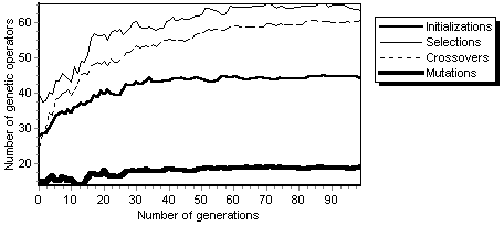
Figure 9.2: The fitness of the best individual in the best run and the average (over 10 runs) of the fitness of the best individual over all runs.

Figure 9.2 shows that the number of the genetic operators used by the best EA increases as the search process advances. For instance the averaged number of Initializations in the best EA from generation 0 is 27, while the averaged number of Initializations in the best evolved EA (after 100 generations) is 43. The averaged number of Mutations is small (less than 18) when compared to the number of occurrences of other genetic operators.

9.3 Evolving evolutionary algorithms with Linear Genetic Programming

In order to use LGP for evolving EAs we have to modify the structure of an LGP chromosome and to define a set of function symbols. This model was proposed in [63].

9.3.1 Individual representation for evolving EAs

Instead of working with registers, our LGP program will modify an array of individuals (the population). In what follows we denote by Pop the array of individuals (the population) which will be modified by an LGP program.

The set of function symbols will consist of genetic operators that may appear into an evolutionary algorithm. Usually, there are 3 types of genetic operators that may appear into an EA. These genetic operators are:

Select - that selects the best solution among several already existing solutions,

Crossover - that recombine two existing solutions,

Mutate - that varies an existing solution.

These operators will act like possible function symbols that may appear into a LGP chromosome. Thus, each simple C instruction that has appeared into a standard LGP chromosome will be replaced by a more complex instruction containing genetic operators. More specific, in the modified LGP chromosomes we may have three major types of instructions. These instructions are:

Pop[$k$] = Select (Pop[$i$], Pop[$j$]); // Select the best individual from those stored in

// Pop[i] and Pop[j] and keep the result in position k.

Pop[$k$] = Crossover (Pop[$i$], Pop[$j$]); // Crossover the individuals stored in Pop[i] and Pop[j]

// and keep the result in position k.

Pop[$k$] = Mutate (Pop[$i$]); // Mutate the individual stored in

// position i and keep the result in position k.

An LGP chromosome $C$, storing an evolutionary algorithm is the following.

void LGP_Program(Chromosome Pop[8]) // a population with 8 individuals

{

…

Pop[0] = Mutate(Pop[5]);

Pop[7] = Select(Pop[3], Pop[6]);

Pop[4] = Mutate(Pop[2]);

Pop[2] = Crossover(Pop[0], Pop[2]);

Pop[6] = Mutate(Pop[1]);

Pop[2] = Select(Pop[4], Pop[3]);

Pop[1] = Mutate(Pop[6]);

Pop[3] = Crossover(Pop[5], Pop[1]);

…

}

These statements will be considered as genetic operations that are executed during an EA generation. Since our purpose is to evolve a generational EA we have to add a wrapper loop around the genetic operations that are executed during an EA generation. More than that, each EA starts with a random population of individuals. Thus, the LGP program must contain some instructions that initialize the initial population.

The obtained LGP chromosome is given below:

void LGP_Program(Chromosome Pop[8]) // a population consisting of 8 individuals

{

Randomly_initialize_the_population();

for (int k = 0; k ¡ MaxGenerations; k++){ // repeat for a fixed

// number of generations

Pop[0] = Mutate(Pop[5]);

Pop[7] = Select(Pop[3], Pop[6]);

Pop[4] = Mutate(Pop[2]);

Pop[2] = Crossover(Pop[0], Pop[2]);

Pop[6] = Mutate(Pop[1]);

Pop[2] = Select(Pop[4], Pop[3]);

Pop[1] = Mutate(Pop[6]);

Pop[3] = Crossover(Pop[5], Pop[1]);

}

}

Remark

The initialization function and the for cycle will not be affected by the genetic operators. These parts are kept unchanged during the search process.

9.3.2 Fitness assignment

We deal with EAs at two different levels: a micro level representing the evolutionary algorithm encoded into a LGP chromosome and a macro level GA, which evolves LGP individuals. Macro level GA execution is bounded by known rules for GAs [9].

For computing the fitness of a LGP individual we have to compute the quality of the EA encoded in that chromosome. For this purpose the EA encoded into a LGP chromosome is run on the particular problem being solved.

Roughly speaking the fitness of a LGP individual is equal to the fitness of the best solution generated by the evolutionary algorithm encoded into that LGP chromosome. But, since the EA encoded into a LGP chromosome use pseudo-random numbers it is very possible as successive runs of the same EA to generate completely different solutions. This stability problem is handled in a standard manner: the EA encoded into a LGP chromosome is executed (run) more times (in fact 200 runs are executed in all the experiments performed for evolving EAs for function optimization and 15 runs for evolving EAs for the TSP) and the fitness of a LGP chromosome is the average of the fitness of the EA encoded in that chromosome over all runs.

Remark

In the standard LGP one of the registers is chosen as the program output. This register is not changed during the search process. In our approach the register storing the best value (best fitness) is chosen to represent the chromosome. Thus, each LGP chromosome stores multiple solutions of a problem in the same manner as Multi Expression Programming [64].

9.3.3 The model used for evolving EAs

For evolving EAs we use the steady state algorithm [95]. For increasing the generalization ability (e.g. the ability of the evolved EA to yield good results on new test problems), the problem set has been divided into three sets, suggestively called training set, validation set and test set (see [86]). In our experiments the training set consists of a difficult test problem. Validation is performed using another difficult test problem. The test set consists of other well-known benchmarking problems.

A method called early stopping is used to avoid overfitting of the population individuals to the particular training examples used [86]. This method consists of computing the test set performance for that chromosome which had the minimum validation error during the search process. Using the early stopping technique will increase the generalization performance [86].

The test set consists of several well-known benchmarking problems [87, 102] used for assessing the performances of the evolutionary algorithms.

9.3.4 Evolving EAs for function optimization

Test functions

Ten test problems $f_{1}-f_{10}$ (given in Table 9.3) are used to asses the performance of the evolved EA. Functions $f_{1}-f_{6}$ are unimodal test function. Functions $f_{7}-f_{10}$ are highly multimodal (the number of local minima increases exponentially with the problem dimension [102]).

Table 9.3: Test functions used in our experimental study. The parameter $n$ is the space dimension ($n$ = 5 in our numerical experiments) and $f_{min}$ is the minimum value of the function.

Test function	Domain	$f_{min}$
$f_{1}(x)=\sum\limits_{i=1}^{n}{(i\cdot x_{i}^{2})}.$	[-5, 5]n	0
$f_{2}(x)=10\cdot n+\sum\limits_{i=1}^{n}{(x_{i}^{2}-10\cdot\cos(2\cdot\pi\cdot x_{i}))}$	[-5, 5]n	0
$f_{3}(x)=-a\cdot e^{-b\sqrt{\frac{\sum\limits_{i=1}^{n}{x_{i}^{2}}}{n}}}-e^{\frac{\sum{\cos(c\cdot x_{i})}}{n}}+a+e.$	[-32, 32]n $a$ = 20, $b$ = 0.2, $c$ = 2$\pi$.	0
$f_{4}(x)=\frac{1}{4000}\cdot\sum\limits_{i=1}^{n}{x_{i}^{2}-\prod\limits_{i=1}^{n}{\cos(\frac{x_{i}}{\sqrt{i}})+1}}.$	[-500, 500]n	0
$f_{5}(x)=\sum\limits_{i=1}^{n}{(-x_{i}\cdot\sin(\sqrt{\left|{x_{i}}\right|}))}$	[-500, 500]n	-$n\quad\bullet$ 418.9829
$f_{6}(x)=\sum\limits_{i=1}^{n}{x_{i}^{2}}.$	[-100, 100]n	0
$f_{7}(x)=\sum\limits_{i=1}^{n}{|x_{i}|+\prod\limits_{i=1}^{n}{|x_{i}|}}.$	[-10, 10]n	0
$f_{8}(x)=\sum\limits_{i=1}^{n}{\left({\sum\limits_{j=1}^{i}{x_{j}^{2}}}\right)}.$	[-100, 100]n	0
$f_{9}(x)=\max_{i}\{x_{i},1\leq i\leq n\}.$	[-100, 100]n	0
$f_{10}(x)=\sum\limits_{i=1}^{n-1}{100\cdot(x_{i+1}-x_{i}^{2})^{2}+(1-x_{i})^{2}}.$	[-30, 30]n	0

Experimental results

In this section we evolve an EA for function optimization and then we asses the performance of the evolved EA. A comparison with a standard GA is performed later in this section.

For evolving an EA we use $f_{2}$ as the training problem and the function $f_{3}$ as the validation problem.

An important issue regards the solutions evolved by the EAs encoded into a LGP chromosome and the specific genetic operators used for this purpose. Solutions evolved by the EA encoded into LGP chromosomes are represented using real values [34]. By initialization, a point within the definition domain is randomly generated. Convex crossover with $\alpha$ = $\raise 2.15277pt\hbox{$\scriptstyle 1$}\kern-1.00006pt/\kern-1.49994pt\lower 1.07639pt\hbox{$\scriptstyle 2$}$ and Gaussian mutation with $\sigma$ = 0.5 are used (for more information on real encoding and specific operators see [19]).

Experiment 1

In this experiment, an EA for function optimization is evolved.

There is a wide range of EAs that can be evolved using the technique described above. Since, the evolved EA has to be compared with another algorithm (such as a standard GA or an ES), the parameters of the evolved EA have to be similar to the parameters of the algorithm used for comparison.

For instance, a standard GA uses a primary population of $N$ individuals and an additional population (the new population) that stores the offspring obtained by crossover and mutation. Thus, the memory requirements for a standard GA is O(2*$N)$. In each generation there will be 2 * $N$ Selections, $N$ Crossovers and $N$ Mutations (we assume here that only one offspring is obtained by crossover of two parents). Thus, the number of genetic operators (Crossovers, Mutations and Selections) in a standard GA is 4 * $N$. We do not take into account the complexity of the genetic operators, since in most of the cases this complexity is different from operator to operator. The standard GA algorithm is given below:

Standard GA algorithm

S₁. Randomly create the initial population P(0)

S₂. for t = 1 to Max_Generations do

S₃. P’(t) = $\phi$;

S₄. for k = 1 to $|$P(t)$|$ do

S₅. p₁ = Select(P(t)); // select an individual from the mating pool

S₆. p₂ = Select(P(t)); // select the second individual

S₇. Crossover (p₁, p₂, offsp); // crossover the parents p₁ and p₂

// the offspring offspr is obtained

S₈. Mutation (offspr); // mutate the offspring offspr

S₉. Add offspf to P’(t);

S₁₀. endfor

S11. P(t+1) = P’(t);

S₁₂. endfor

Rewritten as an LGP program, the Standard GA is given below. The individuals of the standard (main) population are indexed from 0 to PopSize – 1 and the individuals of the new population are indexed from PopSize up to 2 * PopSize – 1.

void LGP_Program(Chromosome Pop[2 * PopSize])

//an array containing of 2 * PopSize individuals

{

Randomly_initialize_the_population();

for (int k = 0; k ¡ MaxGenerations; k++){ // repeat for a fixed

// number of generations

// create the new population

p1 = Select(Pop[3], Pop[6]);

p2 = Select(Pop[7], Pop[7]);

o = Crossover(p1, p2);

Pop[PopSize] = Mutate(o);

p1 = Select(Pop[3], Pop[6]);

p2 = Select(Pop[7], Pop[7]);

o = Crossover(p1, p2);

Pop[PopSize + 1] = Mutate(o);

p1 = Select(Pop[3], Pop[6]);

p2 = Select(Pop[7], Pop[7]);

o = Crossover(p1, p2);

Pop[PopSize + 2] = Mutate(o);

…

p1 = Select(Pop[3], Pop[6]);

p2 = Select(Pop[7], Pop[7]);

o = Crossover(p1, p2);

Pop[2 * PopSize - 1] = Mutate(o);

// pop(t + 1) = new_pop (t)

// copy the individuals from new_pop to the next population

Pop[0] = Pop[PopSize];

Pop[1] = Pop[PopSize];

Pop[2] = Pop[PopSize];

…

Pop[PopSize - 1] = Pop[2 * PopSize - 1];

}

}

The parameters of the standard GA are given in Table 9.4.

Table 9.4: The parameters of a standard GA for Experiment 1.

Parameter	Value
Population size	20 (+ 20 individuals in the new pop)
Individual encoding	Real
Number of generations	100
Crossover probability	1
Crossover type	Convex Crossover with $\alpha$ = 0.5
Mutation	Gaussian mutation with $\sigma$ = 0.01
Selection	Binary Tournament

We will evolve an EA that uses the same memory requirements and the same number of genetic operations as the standard GA described above.

Remark

Our comparison is based on the memory requirements (i.e. the population size) and the number of genetic operators used during the search process. A better comparison could be made if we take into account only the number of function evaluations performed during the search. Unfortunately, this comparison cannot be realized in our model since we cannot control the number of function evaluations (this number is decided by the evolution). The total number of genetic operators (crossovers + mutations + selections) is the only parameter that can be controlled in our model.

The parameters of the LGP algorithm are given in Table 9.5.

Table 9.5: The parameters of the LGP algorithm used for Experiment 1.

Parameter	Value
Population size	500
Code Length	80 instructions
Number of generations	100
Crossover probability	0.7
Crossover type	Uniform Crossover
Mutation	5 mutations per chromosome
Function set	$F$ = {Select, Crossover, Mutate}

The parameters of the evolved EA are given in Table 9.6.

Table 9.6: The parameters of the evolved EA for function optimization.

Parameter	Value
Population size	40
Number of generations	100
Crossover probability	1
Crossover type	Convex Crossover with $\alpha$ = 0.5
Mutation	Gaussian mutation with $\sigma$ = 0.01
Selection	Binary Tournament

The results of this experiment are depicted in Figure 9.3.

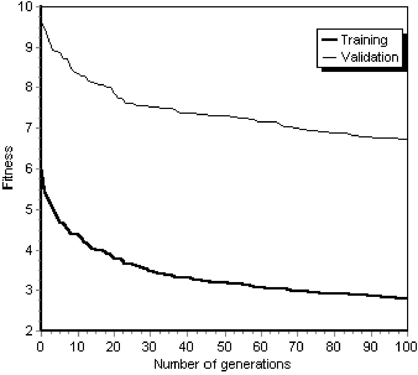
Figure 9.3: The relationship between the fitness of the best individual in each generation and the number of generations. Results are averaged over 10 runs.

Figure 9.3 shows the effectiveness of our approach. LGP technique is able to evolve an EA for solving optimization problems. The quality of the evolved EA improves as the search process advances.

Experiment 2

In this experiment we compare the evolved EA to the standard Genetic Algorithm described in Experiment 1. The parameters used by the evolved EA are given in Table 9.6 and the parameters used by the standard GA are given in Table 9.4. The results of the comparison are given in Table 9.7.

Table 9.7: The results of applying the Evolved EA and the Standard GA for the considered test functions. StdDev stands for the standard deviation. The results are averaged over 30 runs.

Test function	Evolved EA 40 individuals		Standard GA 20 individuals in the standard population + 20 individuals in the new population
	Mean	StdDev	Mean	StdDev
$f_{1}$	0.6152	0.8406	3.1636	3.7997
$f_{2}$	2.6016	1.7073	5.8268	3.9453
$f_{3}$	7.5945	2.5006	10.8979	2.7603
$f_{4}$	2.4639	1.6389	6.0176	4.4822
$f_{5}$	-552.0043	218.8526	-288.3484	200.5584
$f_{6}$	273.7000	235.7794	817.1237	699.2686
$f_{7}$	2.0521	1.1694	4.8836	2.4269
$f_{8}$	340.2770	348.3748	639.2252	486.7850
$f_{9}$	10.3317	4.2009	20.6574	8.8268
$f_{10}$	10123.3083	18645.7247	208900.5717	444827.6967

From Table 9.7 it can be seen that the Evolved EA significantly outperforms the standard GA on all of the considered test problems.

To avoid any suspicion regarding the Evolved EA we will compare it with a GA that uses the same standard population size as the Evolved EA. Thus, the standard GA will use a double population (a standard population and a new population) vis-à-vis the population employed by the Evolved EA. Note that this will provide a significant advantage of the standard GA over the Evolved EA. However, we use this larger population because, in this case, both algorithms (the Standard GA and the Evolved EA) have one important parameter in common: they perform the same number of initializations. Results are presented in Table 9.8.

Table 9.8: The results of applying the Evolved EA and the Standard GA for the considered test functions. StdDev stands for the standard deviation. Results are averaged over 30 runs.

Test function	Evolved EA 40 individuals		Standard GA 40 individuals in the standard population + 40 individuals in the new population
	Mean	StdDev	Mean	StdDev
$f_{1}$	0.6152	0.8406	0.2978	0.5221
$f_{2}$	2.6016	1.7073	3.4031	2.7188
$f_{3}$	7.5945	2.5006	6.2529	2.8255
$f_{4}$	2.4639	1.6389	2.4669	1.5651
$f_{5}$	-552.0043	218.8526	-287.0752	156.5294
$f_{6}$	273.7000	235.7794	263.6049	239.6022
$f_{7}$	2.0521	1.1694	2.0366	1.5072
$f_{8}$	340.2770	348.3748	285.9284	254.9170
$f_{9}$	10.3317	4.2009	10.3776	5.9560
$f_{10}$	10123.3083	18645.7247	9102.8337	23981.1050

Form Table 9.8 it can be seen that the Evolved EA is better than the standard GA in 4 cases (out of 10). However, in this case the standard GA has a considerable advantage over the Evolved EA.

Experiment 3

We are also interested to analyze the relationship between the number of generations of the evolved EA and the quality of the solutions obtained by applying the evolved EA for the considered test functions. The parameters of the Evolved EA (EEA) are given in Table 9.6 and the parameters of the Standard GA (SGA) are given in Table 9.4.

The results of this experiment are depicted in Figure 9.4 (for the unimodal test functions) and in Figure 9.5 (for the multimodal test functions).

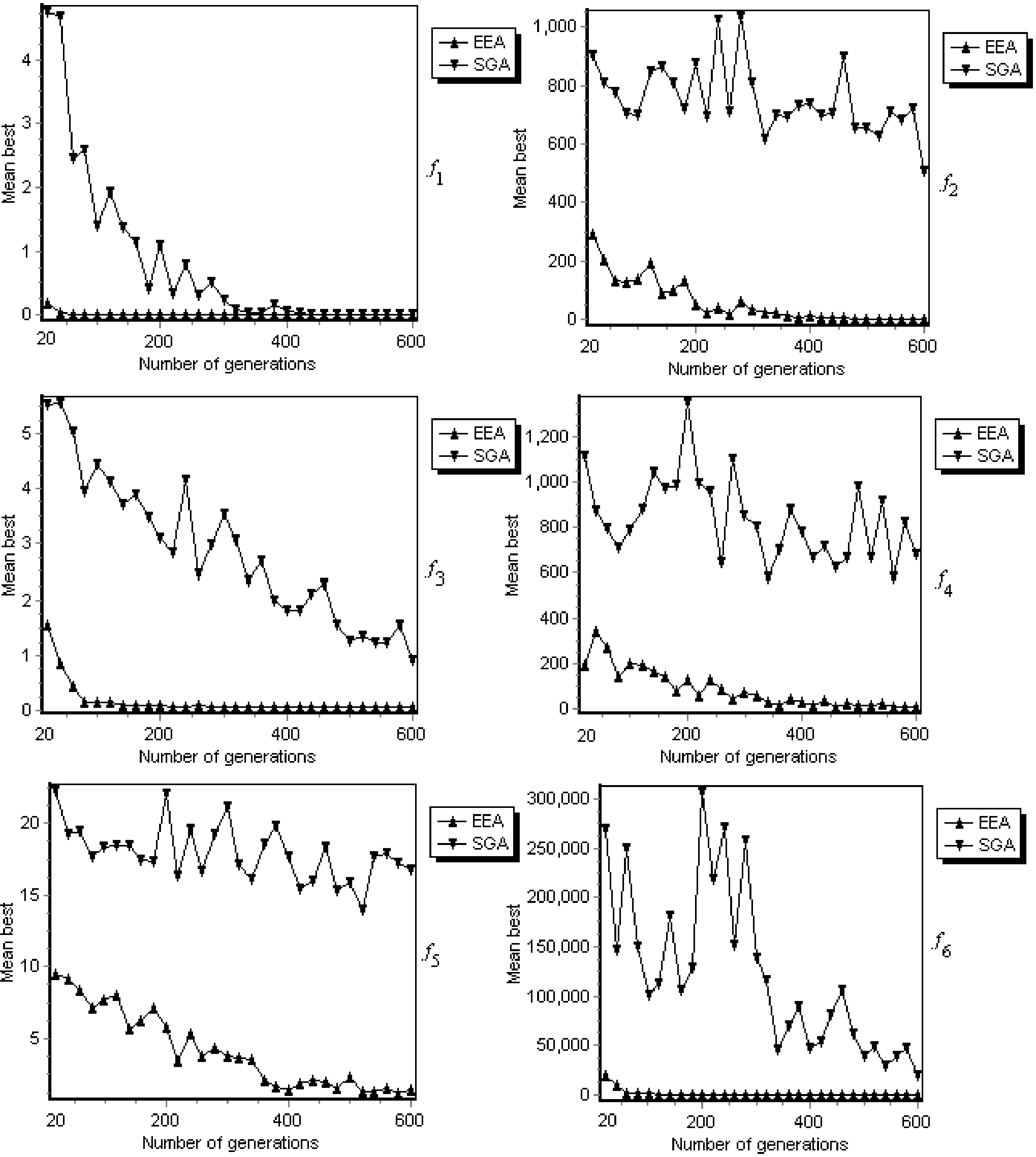
Figure 9.4: The relationship between the number of generations and the quality of the solutions obtained by the Evolved EA (EEA) and by the Standard GA (SGA) for the unimodal test functions $f_{1}-f_{6}$. The number of generations varies between 20 and 600. Results are averaged over 30 runs.

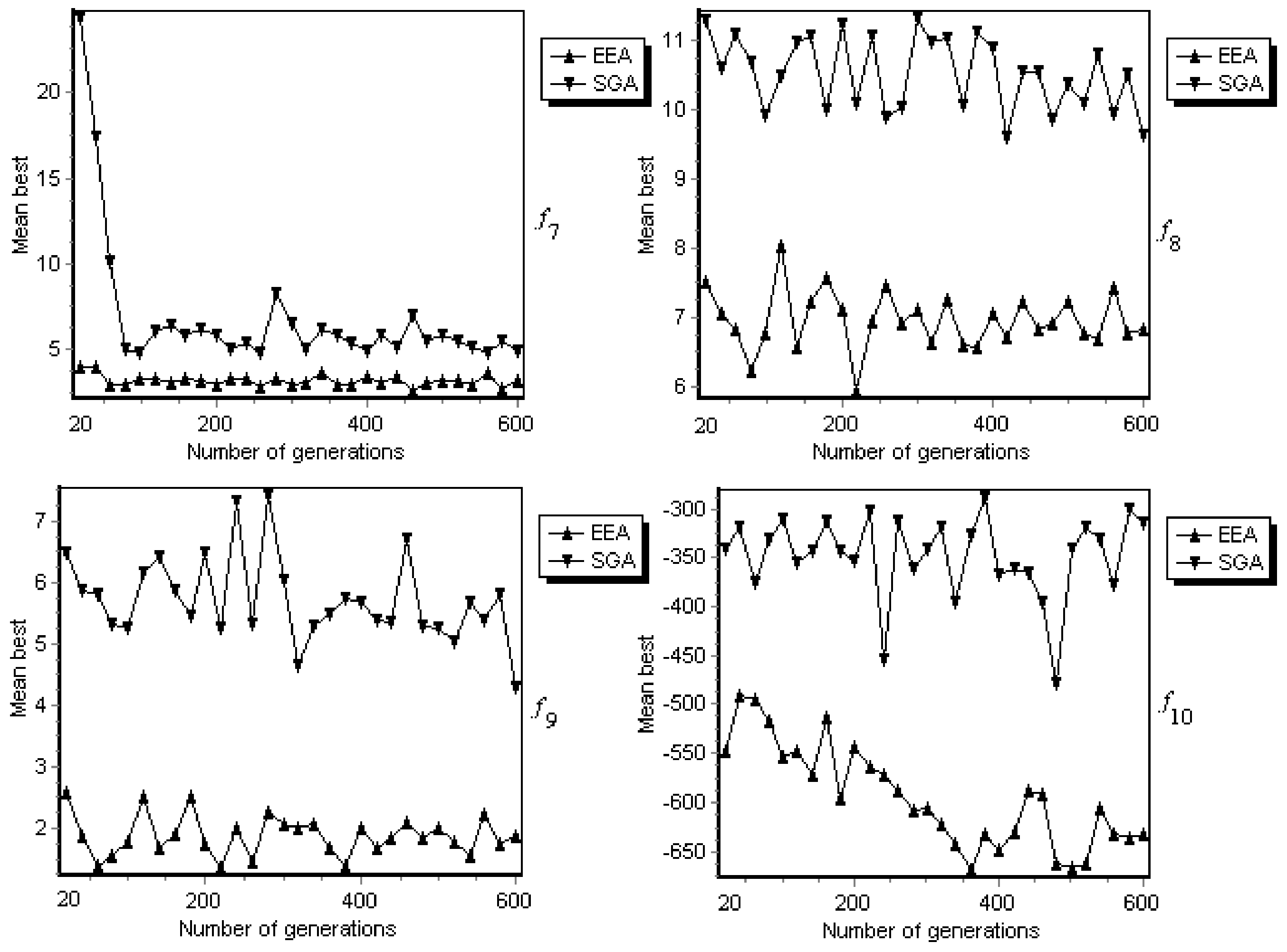
Figure 9.5: The relationship between the number of generations and the quality of the solutions obtained by the Evolved EA (EEA) and by the Standard GA (SGA) for the multimodal test functions $f_{7}-f_{10}$. The number of generations varies between 20 and 600. Results are averaged over 30 runs.

Figures 9.4 and 9.5 show that the Evolved EA is scalable in comparison with the number of generations. It also can be sent that the Evolved EA outperforms the standard GA for all the considered number of generations. For the unimodal test functions ($f_{1}-f_{6})$ we can see a continuous improvement tendency during the search process. For the multimodal test functions we can see a similar behavior only for the test function $f_{10}$.

9.3.5 Evolving EAs for TSP

In this section, an Evolutionary Algorithm for solving the Traveling Salesman Problem [31, 53, 46] is evolved. First of all, an EA is evolved and its performance is assessed by running it on several well-known instances in TSPLIB [87].

This section is entirely original and it is based on the papers [70].

Experiment 5

In this experiment, an EA for the TSP problem is evolved.

A TSP path will be represented as a permutation of cities [51] and it is initialized by using the Nearest Neighbor heuristic [15, 31]. Genetic operators used by the Evolved EA are DPX as crossover [52] and 2-Exchange [46] as mutation. These operators are briefly described in what follows.

DPX recombination operator copies into offspring all the common edges of the parents. Then it completes the offspring to achieve a valid tour with links that do not belong to the parents, in such way that the distance between parents in the newly created offspring is preserved. This completion may be done by using nearest neighbor information [52].

Mutation is done by applying 2-Exchange operator. The 2-Exchange operator breaks the tour by 2 edges and then rebuilds the path by adding 2 new edges (see [46]).

The parameters used by the LGP algorithm are given in Table 9.9.

Table 9.9: The parameters of the LGP algorithm used for Experiment 5.

Parameter	Value
Population size	500
Code Length	80 instructions
Number of generations	50
Crossover probability	0.7
Crossover type	Uniform Crossover
Mutation	5 mutations per chromosome
Function set	$F$ = {Select, Crossover, Mutate}

The parameters of the Evolved EA are given in Table 9.10.

Table 9.10: The parameters of the evolved EA for TSP.

Parameter	Value
Population size	40
Number of generations	100
Crossover probability	1
Crossover type	DPX
Mutation	2-Exchange
Selection	Binary Tournament

For training and testing stages of our algorithm we use several problems from the TSPLIB [86]. The att48 problem (containing 48 nodes) is used for training purposes and the berlin52 problem (containing 52 nodes) is used for validation purposes. Other 25 well-known TSP instances are used as the test set.

Five runs for evolving EAs were performed. A run took about one day on a PIII -600 MHz computer. In each run an EA yielding very good performance has been evolved. One of these EAs has been tested against other 25 difficult instances from TSPLIB. The results of the Evolved EA along with the results obtained with the standard GA described in section 9.3.4 are given in Table 9.11. The standard GA uses a standard population of 40 individuals and an additional population (the new population) with 40 individuals.

Table 9.11: The results of the standard GA and Evolved EA for 27 instances from TSPLIB. Mean stands for the mean over all runs and StdDev stands for the standard deviation. The difference $\Delta$ is in percent and it is computed considering the values of the Evolved EA as a baseline. Results are averaged over 30 runs.

Problem	Standard GA 40 individuals in the standard population + 40 individuals in the new population		Evolved EA 40 individuals		$\Delta$
	Mean	StdDev	Mean	StdDev
a280	3291.18	39.25	3066.72	51.67	7.31
att48	39512.65	883.47	36464.63	780.86	8.35
berlin52	8872.41	145.00	8054.99	128.36	10.14
bier127	129859.76	854.03	128603.46	1058.51	0.97
ch130	7531.64	116.92	6818.78	142.05	10.45
ch150	8087.08	181.14	7019.56	140.01	15.20
d198	18592.67	291.75	17171.83	254.37	8.27
d493	42846.82	686.30	40184.86	544.35	6.62
d657	62348.86	364.76	58421.90	740.38	6.72
eil101	806.03	17.61	734.62	8.60	9.72
eil51	510.81	4.41	470.64	12.19	8.53
eil76	677.55	26.34	599.71	11.46	12.97
fl417	15287.26	159.86	14444.20	268.73	5.83
gil262	2952.11	67.68	2746.59	53.71	7.48
kroA100	25938.18	650.96	23916.58	529.01	8.45
kroA150	33510.69	445.14	30650.92	558.66	9.33
kroA200	35896.96	295.57	34150.88	814.83	5.11
kroB100	27259.50	1295.30	23912.50	346.77	13.99
kroB150	32602.75	590.64	29811.95	519.03	9.36
kroC100	25990.92	453.61	22263.00	585.83	16.74
kroD100	26454.58	864.43	24454.33	383.18	8.17
kroE100	27126.75	667.92	24295.64	517.73	11.65
lin105	19998.93	339.39	16573.09	528.26	20.67
lin318	53525.55	976.88	49778.67	768.35	7.52
p654	45830.71	384.92	41697.25	1356.95	9.91
pcb442	60528.60	294.78	59188.30	677.04	2.26
pr107	48438.22	476.81	46158.41	268.34	4.93

Table 9.11 shows that the Evolved EA performs better than the standard GA for all the considered test problems. The difference $\Delta$ ranges from 0.97 % (for the problem bier127) up to 20.67 % (for the problem lin105).

One can see that the standard GA performs very poor compared to other implementations found in literature [52, 46]. This is due to the weak (non-elitist) evolutionary scheme employed in this experiment. The performance of the GA can be improved by preserving the best individual found so far. However, this is beyond the purpose of this research. Our main aim was to evolve an Evolutionary Algorithm and then to compare it with some similar (in terms of number of genetic operations performed) EA structures.

Experiment 6

In this experiment we use the EA (evolved for function optimization) to solve TSP instances. This transmutation is always possible since the evolved EA does not store any information about the problem being solved. Results are given in Table 9.12.

Table 9.12: The results of the Evolved EA for function optimization (see Appendix 1) and Evolved EA for TSP (see Appendix 2) for 27 instances from TSPLIB. Mean stands for the mean over all runs and StdDev stands for the standard deviation. The difference $\Delta$ is in percent and it is computed considering the values of the Evolved EA for TSP as a baseline. Results are averaged over 30 runs.

Problem	Evolved EA for function optimization 40 individuals		Evolved EA for TSP 40 individuals		$\Delta$
	Mean	StdDev	Mean	StdDev
a280	3156.39	8.54	3066.72	51.67	2.92
att48	39286.76	192.38	36464.63	780.86	7.73
berlin52	8389.56	316.86	8054.99	128.36	4.15
bier127	131069.06	1959.86	128603.46	1058.51	1.91
ch130	7221.11	30.51	6818.78	142.05	5.90
ch150	7094.49	13.57	7019.56	140.01	1.06
d198	18001.13	81.42	17171.83	254.37	4.82
d493	41837.06	492.34	40184.86	544.35	4.11
d657	60844.49	336.61	58421.90	740.38	4.14
eil101	742.77	5.92	734.62	8.60	1.10
eil51	506.59	2.95	470.64	12.19	7.63
eil76	615.68	6.69	599.71	11.46	2.66
fl417	15284.92	64.54	14444.20	268.73	5.82
gil262	2923.88	27.38	2746.59	53.71	6.45
kroA100	25273.13	550.62	23916.58	529.01	5.67
kroA150	31938.69	384.85	30650.92	558.66	4.20
kroA200	35015.95	377.26	34150.88	814.83	2.53
kroB100	25919.43	90.71	23912.50	346.77	8.39
kroB150	31822.17	403.77	29811.95	519.03	6.74
kroC100	23588.58	107.12	22263.00	585.83	5.95
kroD100	25028.15	171.43	24454.33	383.18	2.34
kroE100	25061.34	200.77	24295.64	517.73	3.15
lin105	16977.1	49.02	16573.09	528.26	2.43
lin318	50008.23	413.72	49778.67	768.35	0.46
p654	43689.11	228.15	41697.25	1356.95	4.77
pcb442	59825.62	292.70	59188.30	677.04	1.07
pr107	47718.90	113.56	46158.41	268.34	3.38

From Tables 9.11 and 9.12 it can be seen that the EA evolved for function optimization performs better than the standard GA but worse than the EA evolved for TSP. These results suggest that the structure of an evolutionary algorithm might depend on the problem being solved. This observation is in full concordance with the NFL theorems which tell us that we cannot obtain ”the best” EA unless we embed some information about the problem being solved.

9.4 Conclusions

In this chapter, LGP and MEP have been used for evolving Evolutionary Algorithms. A detailed description of the proposed approaches has been given allowing researchers to apply the method for evolving Evolutionary Algorithms that could be used for solving problems in their fields of interest.

The proposed model has been used for evolving Evolutionary Algorithms for function optimization and the Traveling Salesman Problem. Numerical experiments emphasize the robustness and the efficacy of this approach. The evolved Evolutionary Algorithms perform similar and sometimes even better than some standard approaches in the literature.

Chapter 10 Searching for a Practical Evidence of the No Free Lunch Theorems

A framework for constructing test functions that match a given algorithm is developed in this chapter. More specific, given two algorithms $A$ and $B$, the question is which the functions for which $A$ performs better than $B$ (and vice-versa) are. For obtaining such functions we will use an evolutionary approach: the functions matched to a given algorithm are evolved by using the Genetic Programming (GP) [42] technique.

This chapter is entirely original and it is based on the paper [68, 69].

10.1 Introduction

Since the advent of No Free Lunch (NFL) theorems in 1995 [100], the trends of Evolutionary Computation (EC) [34] have not changed at all, although these breakthrough theories should have produced dramatic changes. Most researchers chose to ignore NFL theorems: they developed new algorithms that work better than the old ones on some particular test problems. The researchers have eventually added: ”The algorithm $X$ performs better than another algorithm on the considered test functions”. That is somehow useless since the proposed algorithms cannot be the best on all the considered test functions. Moreover, most of the functions employed for testing algorithms are artificially constructed.

Consider for instance, the field of evolutionary single-criteria optimization where most of the algorithms were tested and compared on some artificially constructed test functions (most of them being known as De’Jong test problems) [34, 102]. These test problems were used for comparison purposes before the birth of the NFL theorems and they are used even today (8 years later after the birth of the NFL theorems). Evolutionary multi-criteria optimization was treated in a similar manner: most of the recent algorithms in this field were tested on several artificially constructed test functions proposed by K. Deb in [17].

Roughly speaking, the NFL theorems state that all the black-box optimization algorithms perform equally well over the entire set of optimization problems. Thus, if an algorithm $A$ is better than another algorithm $B$ on some classes of functions, the algorithm $B$ is better than $A$ on the rest of the functions.

As a consequence of the NFL theories, even a computer program (implementing an Evolutionary Algorithm (EA)) containing programming errors can perform better than some other highly tuned algorithms for some test functions.

Random search (RS) being a black box search / optimization algorithm should perform better than all of the other algorithms for some classes of test functions. Even if this statement is true, there is no result reported in the specialized literature of a test function for which RS performs better than all the other algorithms (taking into account the NFL restriction concerning the number of distinct solutions visited during the search). However, a function which is hard for all Evolutionary Algorithms is presented in [18].

Three questions (on how we match problems to algorithms) are of high interest:

For a given class of problems, which is (are) the algorithm(s) that performs (perform) better than all other algorithms?

For a given algorithm which is (are) the class(es) of problems for which the algorithm performs best?

Given two algorithms $A$ and $B$, which is (are) the class (es) of problems for which $A$ performs better than $B$?

Answering these questions is not an easy task. All these problems are still open questions and they probably lie in the class of the NP-Complete problems. If this assumption is true it means that we do not know if we are able to construct a polynomial algorithm that takes a function as input and outputs the best optimization algorithm for that function (and vice versa). Fortunately, we can try to develop a heuristic algorithm able to handle this problem.

10.2 Basics on No Free Lunch Theorems

The results provided by the No Free Lunch Theorems are divided in two main classes: No Free Lunch Theorems for Oprimization and No Free Lunch Theorems for Search.

Roughly speaking, the NFL theorems for Optimization [101] state that all the black-box optimization algorithms perform equally well over the entire set of optimization problems.

Thus, if an algorithm $A$ is better than another algorithm $B$ on some classes of functions, the algorithm $B$ is better than $A$ on the rest of the functions.

The NFL theorems for Search [100] state that we cannot use the information about the algorithm’ behaviour so far to predict it’s future behaviour.

10.3 A NFL-style algorithm

Firstly, we define a black-box optimization algorithm as indicated by Wolpert and McReady in [100].

The evolutionary model (the NFL-style algorithm) employed in this study uses a population consisting of a single individual. This considerably simplify the description and the implementation of a NFL-style algorithm. No archive for storing the best solutions found so far (see for instance Pareto Archived Evolution Strategy [45]) is maintained. However, we implicitly maintain an archive containing all the distinct solutions explored until the current state. We do so because only the number of distinct solutions is counted in the NFL theories. This kind of archive is also employed by Tabu Search [32, 33].

The variables and the parameters used by a NFL algorithm are given in Table 10.1.

Table 10.1: The variables used by the NFL algorithm.

Variable	Meaning
Archive	the archive storing all distinct solutions visited by algorithm
curr_sol	the current solution (point in the search space)
new_sol	a new solution (obtained either by mutation or by initialization)
MAX_STpng	the number of generations (the number of distinct points in the search space visited by the algorithm).
$t$	the number of distinct solutions explored so far

The NFL-style algorithm is outlined below:

NFL Algorithm

S₁. Archive = $\emptyset$;

S₂. Randomly initializes the current solution (curr_sol)

// add the current solution to the archive

S₃. Archive = Archive + {curr_sol};

S₄. t = 1;

S₅. while t $<$ MAX_STpng do

S₆. Select a new solution (new_sol) in

the neighborhood of the curr_sol

S₇. Archive = Archive + {new_sol};

S₈. curr_sol = new_sol;

S₉. t = t + 1;

S₁₀. endwhile

An important issue concerning the NFL algorithm described above is related to the step $S_{6}$ which selects a new solution that does not belong to the Archive. This is usually done by mutating the current solution and keeping the offspring if the latter does not already belong to the Archive (The actual acceptance mechanism is minutely described in section 10.5). If the offspring belongs to the Archive for a fixed number of mutations (stpng) it means that the neighborhood of the current solutions could be exhausted (completely explored). In this case, a new random solution is generated and the search process moves to another region of the search space.

It is sometimes possible the generated solution to already belong to the Archive. In this case, another random solution is generated over the search space. We assume that the search space is large enough and after a finite number of re-initializations the generated solution will not belong to the Archive.

The algorithm for selecting a new solution which does not belong to the Archive (the step $S_{6})$ is given below:

SS₁. nr_mut = 0; // the number of mutations is set to 0

SS₂. Repeat

SS₃. new_sol = Mutate (curr_sol);

SS₄. nr_mut = nr_mut + 1;

SS₅. until (nr_mut = MAX_MUTATIONS) and (new_sol $\notin$Archive) and Accepted(new_sol);

SS₆. while new_sol $\notin$Archive do

SS₇. Initialize(new_sol); //we jump into another randomly chosen point of the search space

SS₈. endwhile

10.4 Evolutionary Model and the Fitness Assignment Process

Our aim is to find a test function for which a given algorithm $A$ performs better than another given algorithm $B$. The test function that is being searched for will be evolved by using Genetic Programming [42] with steady state [95].

The quality of the test function encoded in a GP chromosome is computed in a standard manner. The given algorithms $A$ and $B$ are applied to the test function. These algorithms will try to optimize (find the minimal value of) that test function. To avoid the lucky guesses of the optimal point, each algorithm is run 500 times and the results are averaged. Then, the fitness of a GP chromosome is computed as the difference between the averaged results of the algorithm $A$ and the averaged results of the algorithm $B$. In the case of function minimization, a negative fitness of a GP chromosome means that the algorithm $A$ performs better than the algorithm $B$ (the values obtained by $A$ are smaller (on average) than those obtained by $B)$.

10.5 Algorithms used for comparison

We describe several evolutionary algorithms used for comparison purposes. All the algorithms described in this section are embedded in the NFL algorithm described in section 10.3. More precisely, the considered algorithms particularize the solution representation, the mutation operator, and the acceptance mechanism (the procedure Accepted) of the NFL algorithm described in section 10.3. The mutation operator is the only search operator used for exploring the neighborhood of a point in the search space.

A₁ - real encoding (the individuals are represented as real numbers using 32 bits), Gaussian mutation with $\sigma_{1}$ = 0.001, the parent and the offspring compete for survival.

A₂ - real encoding (the individuals are represented as real numbers using 32 bits), Gaussian mutation with $\sigma_{2}$ = 0.01, the parent and the offspring compete for survival.

A₃ - binary encoding (the individuals are represented as binary strings of 32 bits), point mutation with $p_{m}$ = 0.3, the parent and the offspring compete for survival.

A₄ - binary encoding (the individuals are represented as binary strings of 32 bits), point mutation with $p_{m}$ = 0.1, the parent and the offspring compete for survival.

10.6 Numerical experiments

Several numerical experiments for evolving functions matched to a given algorithm are performed in this section. The algorithms used for comparison have been described in section 10.5.

The number of dimensions of the space is set to 1 (i.e. one-dimensional functions) and the definition domain of the evolved test functions is [0, 1].

The parameters of the GP algorithm are given in Table 10.2.

Table 10.2: The parameters of the GP algorithm used for numerical experiments

Parameter	Value
Population size	50
Number of generations	10
Maximal GP tree depth	6
Function set	$F$ = {+, -, *, sin, exp}
Terminal set	$T$ = {$x$}
Crossover probability	0.9
Mutation	1 mutation / chromosome
Runs	30

The small number of generations (only 10) has been proved to be sufficient for the experiments performed in this study.

Evolved functions are given in Table 10.3. For each pair ($A_{k}$, $A_{j})$ is given the evolved test function for which the algorithm $A_{k}$ performs better than the algorithm $A_{j}$. The mean of the fitness of the best GP individual over 30 runs is also reported.

Table 10.3: The evolved test functions.

Algorithms	Evolved Test Function	Averaged fitness
($A_{1}$, $A_{2})$	$f_{1}(x)=0.$	0
($A_{2}$, $A_{1})$	$f_{2}(x)=-6x^{3}-x.$	-806.03
($A_{3}$, $A_{4})$	$f_{3}(x)=x-2x^{5}.$	-58.22
($A_{4}$, $A_{3})$	$f_{4}(x)=-4x^{8}.$	-34.09
($A_{2}$, $A_{4})$	$f_{5}(x)=0.$	0
($A_{4}$, $A_{2})$	$f_{6}(x)=-6x^{3}-x.$	-1601.36

Table 10.3 shows that the proposed approach made possible the evolving of test functions matched to the most of the given algorithms. The results of these experiments give a first impression of how difficult the problems are. Several interesting observations can be made:

The GP algorithm was able to evolve a function for which the algorithm $A_{2}$ (real encoding with $\sigma$ = 0.01) was better then the algorithm $A_{1}$ (real encoding with $\sigma$ = 0.001) in all the runs (30). However, the GP algorithm was not able to evolve a test function for which the algorithm $A_{1}$ is better that the algorithm $A_{2}$. In this case the function $f(x)$ = 0 (where both algorithms perform the same) was the only one to be found. It seems to be easier to find a function for which an algorithm with larger ”jumps” is better than an algorithm with smaller ”jumps” than to find a function for which an algorithm with smaller ”jumps” is better than an algorithm with larger ”jumps”.

A test function for which the algorithm $A_{4}$ (binary encoding) is better than the algorithm $A_{2}$ (real encoding) was easy to find. The reverse (i.e. a test function for which the real encoding algorithm $A_{2}$ is better than the binary encoded algorithm $A_{4})$ has not been found by using the GP parameters considered in Table 10.2.

10.7 Conclusions and further work

In this paper, a framework for evolving test functions that are matched to a given algorithm has been proposed. The proposed framework is intended to provide a practical evidence for the NFL theories. Numerical experiments have shown the efficacy of the proposed approach.

Further research will be focused on the following directions:

• extending the function set ($F)$ and the number of space dimensions.

• comparing other evolutionary algorithms for single and multiobjective optimization. Several test functions matched to some classical algorithms (such as standard GAs or ES) for function optimization will be evolved. In this case the problem is much more difficult since the number of distinct solutions visited during the search process could be different for each algorithm.

• evolving test instances for algorithms used for solving other real-world problems (such as TSP, symbolic regression, classification etc).

• finding test functions for which random search is better than other algorithms.

• finding the set of test functions for which an algorithm is better than the other.

Chapter 11 Conclusions and further work

Three new techniques have been proposed during the course of this thesis: Multi Expression Programming, Infix Form Genetic Programming, and Traceless Genetic Programming.

Proposed techniques have been used in the following applications: symbolic regression, classification, designing digital circuits, evolving play strategies, evolving heuristics for NP-complete problems, evolving evolutionary algorithms, and evolving test problems.

Further work will be focused on developing new GP techniques, Designing digital circuits for reversible computers, evolving fast winning strategies for the end of the chess and othello games, evolving EAs with patterns, evolving heuristics for other NP-complete problems, applying the existing GP techniques to real-world prediction data, etc.

Bibliography

- [1] Aarts, E.H.L., Lenstra, J. K. (Editors), Local Search in Combinatorial Optimization, John Wiley and Sons, London, 1997.
- [2] Aho, A., Sethi R., Ullman J., Compilers: Principles, Techniques, and Tools, Addison Wesley, 1986.
- [3] Angeline, P.J., Two Self-Adaptive Crossover Operators for Genetic Programming, In Advances in Genetic Programming II, Edited by Angeline, P.J. and Kinnear, K.E., pp. 89-110, MIT Press, 1996.
- [4] Banzhaf, W., Nordin, P., Keller, E. R., Francone, F. D., Genetic Programming - An Introduction, Morgan Kaufmann, San Francisco, CA, 1998.
- [5] Back, T., Evolutionary Algorithms in Theory and Practice, Oxford University Press, Oxford, 1996.
- [6] Back, T., Fogel, D.B., Michalewicz, Z. (Eds.), Handbook of Evolutionary Computation, Institute of Physics Publishing, Bristol, and Oxford University Press, New York, 1997.
- [7] Bellman, R., Dynamic Programming, Princeton, Princeton University Press, New Jersey, 1957.
- [8] Berlekamp, E. R., Conway J. H., Guy R. K., Winning Ways for Your Mathematical Plays, Academic Press, London, 1982.
- [9] Brameier, M., Banzhaf, W., A Comparison of Linear Genetic Programming and Neural Networks in Medical Data Mining, IEEE Transactions on Evolutionary Computation, Vol. 5, pp. 17-26, IEEE Press, NY, 2001.
- [10] Brameier, M., Banzhaf, W., Explicit Control of Diversity and Effective Variation Distance in Linear Genetic Programming, In Proceedings of the European Conference on Genetic Programming, Edited by Lutton, E., Foster, J., Miller, J., Ryan, C., and Tettamanzi, A., Springer-Berlin, pp. 38-50, 2002.
- [11] Brameier, M., Banzhaf, W., Evolving Teams of Predictors with Linear Genetic Programming, Genetic Programming and Evolvable Machines, Vol. 2, pp. 381-407, 2001.
- [12] Chellapilla, K., Fogel, D. B., Evolution, Neural Networks, Games and Intelligence, Proceedings of the IEEE, pp. 1471-1496, 2000.
- [13] Coello, C., Alba, E., Luque, G., Aguire A., Comparing different Serial and Parallel Heuristics to Design Combinational Logic Circuits, In Proceedings of 2003 NASA/DoD Conference on Evolvable Hardware, J. Lohn, R. Zebulum, J. Steincamp, D. Keymeulen, A. Stoica, M.I. Ferguson, pp. 3-12, 2003.
- [14] Conway, J. H., On Numbers and Games, Academic Press, London, 1976.
- [15] Cormen, T.H., Leiserson, C.E. Rivest, R. R., Introduction to Algorithms, MIT Press, Cambridge, MA, 1990.
- [16] Cramer, N.L., A representation for the adaptive generation of sequencial programs, In Proceedings of the Workshop on Genetic Algorithms: From Theory to Real-World Applications, pp. 183-187, 1985.
- [17] Deb, K., Multi-Objective Genetic Algorithms: Problem Difficulties and Construction of Test Functions, Evolutionary Computation, Vol. 7, pp. 205-230 , MIT Press, Cambridge, MA, 1999.
- [18] Droste, S., Jansen, T., Wegener, I., A Natural and Simple Function which is Hard for All Evolutionary Algorithms, technical report, Univ. Dortmund, Germany, 2000.
- [19] Dumitrescu, D., Lazzerini, B., Jain, L., Dumitrescu, A., Evolutionary Computation. CRC Press, Boca Raton, FL, 2000.
- [20] Dumitrescu, D., Oltean, M., Proving Theorems using Genetic Programming, Studia, Ser. Informatica, Babeş-Bolyai University, 1999.
- [21] Dumitrescu, D., Groşan, C., Oltean, M., Evolving Pareto Continuous Regions, Evolutionary Computation Based Multi-Criteria Optimization: Theoretical Advances and Applications, A. Abraham, L. Jain and R. Goldberg, (editors), Springer-Verlag, London, 2004.
- [22] Edmonds, B., Meta-Genetic Programming: Co-evolving the Operators of Variation. Electrik, Vol. 9, pp. 13-29, 2001.
- [23] Ferreira, C., Gene Expression Programming: a New Adaptive Algorithm for Solving Problems, Complex Systems, Vol. 13, Nr. 1, pp. 87-129, 2001.
- [24] Ferreira, C., Mutation, Transposition, and Recombination: An Analysis of the Evolutionary Dynamics. In H. J. Caulfield, S.-H. Chen, H.-D. Cheng, R. Duro, V. Honavar, E. E. Kerre, M. Lu, M. G. Romay, T. K. Shih, D. Ventura, P. P. Wang, Y. Yang, eds., Proceedings of the 6th Joint Conference on Information Sciences, 4th International Workshop on Frontiers in Evolutionary Algorithms, pp. 614-617, Research Triangle Park, North Carolina, USA, 2002.
- [25] Ferreira, C., Discovery of the Boolean Functions to the Best Density-Classification Rules Using Gene Expression Programming. In E. Lutton, J. A. Foster, J. Miller, C. Ryan, and A. G. B. Tettamanzi, eds., Proceedings of the 4th European Conference on Genetic Programming, EuroGP 2002, LNCS 2278, pp. 51-60, Springer-Verlag, Berlin, Germany, 2002.
- [26] Ferreira, C., 2002. Genetic Representation and Genetic Neutrality in Gene Expression Programming. Advances in Complex Systems, Vol. 5 Nr. 4 pp. 389-408, 2002.
- [27] Fogel, D.B., Evolutionary Computation, IEEE Press, New-York, 1995.
- [28] Fraenkel, S., Scenic Trails Ascending from Sea-Level Nim to Alpine Chess, Games of No Chance, MSRI Publications, Vol. 29, 1996.
- [29] Freisleben, B. Merz, P., A Genetic Local Search Algorithm for Solving Symmetric and Asymmetric Traveling Salesman Problems, In Proceedings of the 1996 IEEE International Conference on Evolutionary Computation, pp. 616-621, 1996.
- [30] Gardner, M., Hexaflexagons and Other Mathematical Diversions, The University of Chicago Press, 1988.
- [31] Garey, M.R., Johnson D.S., Computers and Intractability: A Guide to NP-completeness, Freeman & Co, San Francisco, 1979.
- [32] Glover, F., Tabu search - Part I, ORSA Journal of Computing, 1, (1989), 190-206
- [33] Glover, F., Tabu search - Part II, ORSA Journal of Computing, 2, (1990), 4-32
- [34] Goldberg, D.E., Genetic Algorithms in Search, Optimization, and Machine Learning, Addison-Wesley, Reading, MA, 1989.
- [35] Groşan, C., Oltean, M., Adaptive Representation for Single Objective Optimization, First Balkan Conference on Informatics, 17-20 November 2003, Tesalonik, Greece, Y. Manoulopulus (editor), pp. 345-355, 2003.
- [36] Groşan C., Oltean M., Adaptive Representation for Single Objective Optimization, Soft Computing, Springer-Verlag, 2004 (Accepted).
- [37] Handley, S., On the Use of a Directed Graph to Represent a Population of Computer Programs. Proceeding of the IEEE World Congress on Computational Intelligence, pp. 154-159, Orlando, Florida, 1994.
- [38] Haykin, S., Neural Networks, a Comprehensive Foundation, second edition, Prentice-Hall, Englewood Cliffs, 1999.
- [39] Holland, J.H., Adaptation in Natural and Artificial Systems, University of Michigan Press, Ann Arbor, 1975.
- [40] Kantschik, W., Banzhaf, W., Linear-Tree GP and its comparison with other GP structures, In J. Miller, M. Tomassini, P.-L. Lanzi, C. Ryan, A. Tettamanzi and W. B. Langdon editors, Proceedings of 4th EuroGP Conference, Springer, pp. 302-312, 2001.
- [41] Joza, J.R. Hierarchical genetic algorithms operating on populations of computer programs. In Proceedings of the Eleventh International Joint Conference on Artificial Intelligence IJCAI-89, pp. 768-774, Morgan-Kaufmann, San-Francisco, CA, 1989.
- [42] Koza, J. R., Genetic Programming: On the Programming of Computers by Means of Natural Selection, MIT Press, Cambridge, MA, 1992.
- [43] Koza, J. R., Genetic Programming II: Automatic Discovery of Reusable Subprograms, MIT Press, Cambridge, MA, 1994.
- [44] Koza, J. R. et al., Genetic Programming III: Darwinian Invention and Problem Solving, Morgan Kaufmann, San Francisco, CA, 1999.
- [45] Knowles, J. D., Corne, D.W.: Approximating the Nondominated Front using the Pareto Archived Evolution Strategies, Evolutionary Computation, Vol. 8, pp. 149-172, MIT Press, Cambridge, MA, 2000.
- [46] Krasnogor, N., Studies on the Theory and Design Space of Memetic Algorithms, PhD Thesis, University of the West of England, Bristol, 2002.
- [47] Krasnogor, N., Smith, J.E., A Memetic Algorithm with Self-Adaptive Local Search: TSP a Case Study, In Proceedings of 2000 Genetic and Evolutionary Computation Conference, Morgan Kaufmann, 2000.
- [48] Langdon, W. B., Poli, R., Genetic Programming Bloat with Dynamic Fitness. W. Banzhaf, R. Poli, M. Schoenauer, and T. C. Fogarty (editors), Proceedings of the First European Workshop on Genetic Programming, pp. 96-112, Springer-Verlag, Berlin, 1998.
- [49] Lones, M.A., Tyrrell, A.M., Biomimetic Representation in Genetic Programming, Proceedings of the Workshop on Computation in Gene Expression at the Genetic and Evolutionary Computation Conference 2001 (GECCO2001), July 2001.
- [50] McPhee, N. F., Hopper N. J., Analysis of Genetic Diversity through Population History, Proceedings of the Genetic and Evolutionary Computation Conference, W. Banzhaf, J. Daida, A. E. Eiben, M. H. Garzon, V. Honavar, M. Jakiela, and R. E. Smith, (editor) pp. 1112-1120, Morgan Kaufmann, 1999.
- [51] Merz, P., Freisleben, B., A Genetic Local Search Approach to the Quadratic Assignment Problem, in Proceedings of the 7th International Conference on Genetic Algorithms, Back T. (Editors), pp. 465–472, Morgan Kaufmann, 1997.
- [52] Merz, P., Freisleben, B., Genetic Local Search for the TSP: New Results, in Proceedings of the IEEE International Conference on Evolutionary Computation, Back T., Michalewicz Z. and Yao X. (Editors), pp. 159-164, IEEE Press, 1997.
- [53] Merz, P., Freisleben, B., Memetic Algorithms for the Traveling Salesman Problem, Complex-Systems, Vol 13, 2003.
- [54] Miller, J. F., Thomson, P., Aspects of Digital Evolution: Evolvability and Architecture. In Proceedings of the Parallel Problem Solving from Nature V, A. E. Eiben, Bäck T., Schoenauer M. and Schwefel H-P. (Editors), pp. 927-936, Springer, 1998.
- [55] Miller, J.F., Thomson, P., Cartesian Genetic Programming. In Proceedings of the 3rd International Conference on Genetic Programming (EuroGP2000), R. Poli, J.F. Miller, W. Banzhaf, W.B. Langdon, J.F. Miller, P. Nordin, T.C. Fogarty (Editors), LNCS 1802, Springer-Verlag, Berlin, pp. 15-17, 2000.
- [56] Miller, J. F., Thomson, P., Fogarty, T., Designing Electronic Circuits using Evolutionary Algorithms. Arithmetic Circuits: A Case Study. In Genetic Algorithms and Evolution Strategies in Engineering and Computer Science, Quagliarella D., Periaux J., Poloni C. and G. Winter (Editors), pp. 105–131, Chechester, UK-Wiley, 1997.
- [57] Miller, J. F., An Empirical Study of the Efficiency of Learning Boolean Functions using a Cartesian Genetic Programming Approach. In Proceedings of the 1st Genetic and Evolutionary Computation Conference, Banzhaf W., Daida J., Eiben A. E., Garzon M. H., Honavar V., Jakiela M., and Smith R. E., (editors), Vol. 2, pp. 1135–1142, Morgan Kaufmann, San Francisco, CA, 1999.
- [58] Miller, J. F., Job, D., Vassilev, V.K., Principles in the Evolutionary Design of Digital Circuits - Part I, Genetic Programming and Evolvable Machines, Vol. 1(1), pp. 7–35, Kluwer Academic Publishers, 2000.
- [59] Mitchell, T., Machine Learning, McGraw-Hill, New-York, 1996.
- [60] Moscato, P., On Evolution, Search, Optimization, Genetic Algorithms and Martial Arts: Towards Memetic Algorithms, Tech. Rep. Caltech Concurrent Computation Program, Report. 826, California Institute of Technology, Pasadena, California, USA, 1989.
- [61] Moscato, P. Norman, M. G., A Memetic Approach for the Traveling Salesman Problem Implementation of a Computational Ecology for Combinatorial Optimization on Message-Passing Systems, in Parallel Computing and Transputer Applications, Valero M., Onate E., Jane M., Larriba J. L., and Suarez B. (editor), pp. 177–186, IOS Press, Amsterdam, 1992.
- [62] Nordin, P., A Compiling Genetic Programming System that Directly Manipulates the Machine Code, K. E. Kinnear, Jr. (editor), Advances in Genetic Programming, pp. 311-331, MIT Press, 1994.
- [63] Oltean, M., Evolving Evolutionary Algorithms for Function Optimization, in Proceedings of the International Conference on Information Sciences, 26-30 September 2003, North Carolina, K. Chen (editor), pp. 295-298, 2003.
- [64] Oltean, M., Dumitrescu, D., Multi Expression Programming, technical report, Babes-Bolyai University, (available at www.mep.cs.ubbcluj.ro), 2002.
- [65] Oltean, M., Groşan C., Evolving Evolutionary Algorithms using Multi Expression Programming, The European Conference on Artificial Life, Dortmund, 14-17 September, W. Banzhaf (editor), LNAI 2801, pp. 651-658, Springer-Verlag, Berlin, 2003.
- [66] Oltean, M., Solving Even-parity problems with Multi Expression Programming, Te 8th International Conference on Computation Sciences, 26-30 September 2003, North Carolina, K. Chen (editor), pp. 315-318, 2003.
- [67] Oltean, M., Groşan, C., Solving Classification Problems using Infix Form Genetic Programming, The International Symposium on Intelligent Data Analysis, August 28-30, 2003, Berlin, M. Berthold (editor), LNCS 2810, pp. 242-252, Springer, Berlin, 2003.
- [68] Oltean, M., A Practical Evidence for the No Free Lunch Theorems, BioInspired Approaches to Advanced Information Technology, BioADIT’04, Lausanne, Switzerland, 29-31 January, A. Ijspeert et al. (editors), pp. 482-488, 2004.
- [69] Oltean, M., Searching for a Practical Evidence for the No Free Lunch Theorems, BioInspired Approaches to Advanced Information Technology, BioADIT’04, Lausanne, Switzerland, 29-31 January, A. Ijspeert (editor), LNCS 3141, Springer-Verlag, Berlin, pp. 395-406, 2004.
- [70] Oltean, M., Dumitrescu, D., Evolving TSP Heuristics using Multi Expression Programming, International Conference on Computational Sciences, ICCS’04, M. Bubak, G. D. van Albada, P. Sloot, and J. Dongarra (editors), Vol II, pp. 670-673, 6-9 June, Krakow, Poland, 2004.
- [71] Oltean, M., Evolving Digital Circuits for the Knapsack Problem, International Conference on Computational Sciences, M. Bubak, G. D. van Albada, P. Sloot, and J. Dongarra (editors), Vol. III, pp. 1257-1264, 6-9 June, Krakow, Poland, 2004.
- [72] Oltean, M., Dumitrescu, D., A Permutation based Approach for the 2-D Cutting Stock Problem, First International Industrial Conference Bionik 2004, Edited by Boblan, I. and Bannasch, R., 22-23 April, Hannover, Germany, pp. 73-80, 2004.
- [73] Oltean, M., Solving Even-Parity Problems using Traceless Genetic Programming, IEEE Congress on Evolutionary Computation, Portland, 19-23 June, G. Greenwood (editor), pages 1813-1819, IEEE Press, 2004.
- [74] Oltean, M., Encoding Multiple Solutions in a Linear GP Chromosome, International Conference on Computational Sciences, M. Bubak, G. D. van Albada, P. Sloot, and J. Dongarra (editors), Vol III, pp. 1281-1288, 6-9 June, Krakow, Poland, 2004.
- [75] Oltean, M., Groşan, A Comparison of Several Linear Genetic Programming Techniques, Complex-Systems, Vol. 14, Nr. 4, pp. 282-311, 2003.
- [76] Oltean, M., Evolving Winning Strategies for Nim-like Games, World Computer Congress, Student Forum, 26-29 August, Toulouse, France, edited by Mohamed Kaaniche, pp. 353-364, Kluwer Academic Publisher, 2004.
- [77] Oltean, M., Solving Classification Problems using Traceless Genetic Programming, World Computer Congress, The Symposium on Profesional Practice in AI, 26-29 August, Toulouse, France, edited by E. Mercier-Laurent, J. Debenham, pp. 403-412, 2004.
- [78] Oltean M., Improving the Search by Encoding Multiple Solutions in a Chromosome, contributed chapter 15, Evolutionary Machine Design, Nova Science Publisher, New-York, N. Nedjah, L. de Mourrelo (editors), 2004.
- [79] Oltean M., Grosan C., Evolving Digital Circuits using Multi Expression Programming, NASA/DoD Conference on Evolvable Hardware, 24-25 June, Seatle, R. Zebulum, D. Gwaltney, G. Horbny, D. Keymeulen, J. Lohn, A. Stoica (editors), pages 87-90, IEEE Press, NJ,2004.
- [80] Oltean M., Improving Multi Expression Programming: an Ascending Trail from Sea-Level Even-3-Parity to Alpine Even-18-Parity, chapter 10, Evolutionary Machine Design: Theory and Applications, Springer-Verlag, N. Nedjah and L. de Mourrelo (editors), pp. 270-306, 2004.
- [81] Oltean, M., Evolving Evolutionary Algorithms using Linear Genetic Programming, Evolutionary Computation, MIT Press, MA, USA, 2005 (accepted).
- [82] O’Neill, M. Ryan, C., Grammatical Evolution, IEEE Transaction on Evolutionary Computation, Vol 5, 2001.
- [83] O’Reilly, U.M., Oppacher, F., A Comparative Analysis of Genetic Programming, Advances in Genetic Programming 2, Peter J. Angeline and Kenneth E. Kinnear (editors), pp. 23-44, MIT Press, 1996.
- [84] Patterson, N.R., Genetic Programming with Context-Sensitive Grammars, PhD thesis, University of St Andrews, Scotland, 2003.
- [85] Poli, R., Langdon, W. B., Sub-machine Code Genetic Programming, Technical report CSRP-98-18, School of Computer Science, University of Birmingham, 1998.
- [86] Prechelt, L., PROBEN1 – A Set of Neural Network Problems and Benchmarking Rules, Technical Report 21, University of Karlsruhe, 1994.
- [87] Reinelt, G., TSPLIB – A Traveling Salesman Problem Library, ORSA, Journal of Computing, Vol. 3(4), pp. 376-384, 1991.
- [88] Rechenberg, I., Evolutionsstrategie’94, Frommann-Holzboog, 1994.
- [89] Samuel, A., Some studies in machine learning using the game of checkers, In Computers and Thought, Feigenbaum, E., and Feldman, J., (editors), McGraw-Hill, New-York, 1963.
- [90] Spector, L., Robinson, A., Genetic Programming and Autoconstructive Evolution with the Push Programming Language, Genetic Programming and Evolvable Machines, Vol.3, Nr.1 pp. 7-40, 2002.
- [91] Stoica, A., Zebulum, R., Guo, X., Keymeulen, D., Ferguson, M. Duong, V., Silicon Validation of Evolution Designed Circuits, In Proceedings of the 2003 NASA/DoD Conference on Evolvable Hardware, pp. 21-26, 2003.
- [92] Stoica, A., Zebulum, R. S., Xin Guo, Keymeulen, D., Ferguson, M. I., Duong, V., Taking Evolutionary Circuit Design from Experimentation to Implementation: some useful Techniques and a Silicon Demonstration, In IEE Proceedings Computers and Digital Techniques (Special Issue on Evolvable Hardware), 2003.
- [93] Stoica, A., Zebulum, R. S., Xin Guo, Keymeulen, D., Ferguson, M. I., Scalability Issues in Evolutionary Synthesis of Electronic Circuits Lessons Learned and Challenges ahead Computational Synthesis Workshop, AAAI Spring Symposium Series, Stanford University, CA, pp. 233-238, 2003.
- [94] Streeter M.J. Two Broad Classes of functions for Which a No Free Lunch Result does not Hold, In Proceedings of the GECCO 2003, edited by Erick Cantu-Paz (et al), 1418-1430, Springer, 2003.
- [95] Syswerda, G., Uniform Crossover in Genetic Algorithms, Schaffer, J.D., (editor), Proceedings of the 3rd International Conference on Genetic Algorithms, pp. 2-9, Morgan Kaufmann Publishers, San Mateo, CA, 1989.
- [96] Tatar, D., Oltean, M., Proving Theorems using DNA, Studia, Ser. Informatica, Babeş-Bolyai University, 1999.
- [97] Teller, A., Evolving Programmers: the Co-evolution of Intelligent Recombination Operators, in Advances in Genetic Programming II, Angeline P. and Kinnear K.E., (editors), MIT Press, pp. 45-68, 1996.
- [98] Whitley, L.D., A Free Lunch Proof for Gray versus Binary Encodings, in Proceedings of the Genetic and Evolutionary Computation Conference, W. Banzhaf J., Daida, A. E. Eiben M. H. Garzon, V. Honavar M. Jakiela, R. E. Smith (editors) Vol. 1, Morgan Kaufmann, pp. 726-733, 1999.
- [99] Whitley, L.D., Functions as Permutations: Implications for No Free Lunch, Walsh Analysis and Statistics, in Proc. of the Sixth International Conference on Parallel Problem Solving from Nature (PPSN VI), Schoenauer, M., Deb, K., Rudolph, G., Yao, X., Lutton, E., Merelo, J.J. and Schwefel, H.-P. (editors) , Springer Verlag, Berlin, pp. 169-178, 2000.
- [100] Wolpert, D.H., McReady, W.G., No Free Lunch Theorems for Search, technical report SFI-TR-05-010, Santa Fe Institute, 1995.
- [101] Wolpert, D.H., McReady, W.G., No Free Lunch Theorems for Optimisation, IEEE Transaction on Evolutionary Computation, Vol. 1, pp. 67-82, 1997.
- [102] Yao, X., Liu, Y., Lin, G., Evolutionary Programming Made Faster, IEEE Transaction on Evolutionary Computation, Vol. 3(2), pp. 82-102, 1999.
- [103] UCI Machine Learning Repository, Available from www.ics.uci.edu/mlearn/MLRepository.html