SteParSyn: A Bayesian code to infer stellar atmospheric parameters using spectral synthesis

Abstract

Context. SteParSyn is an automatic code written in Python 3.X designed to infer the stellar atmospheric parameters $T_{\rm eff}$, $\log{g}$, and [Fe/H] of FGKM-type stars following the spectral synthesis method.

Aims. We present a description of the SteParSyn code and test its performance against a sample of late-type stars that were observed with the HERMES spectrograph mounted at the 1.2-m Mercator Telescope. This sample contains 35 late-type targets with well-known stellar parameters determined independently from spectroscopy. The code is available to the astronomical community in a GitHub repository.

Methods. SteParSyn uses a Markov chain Monte Carlo (MCMC) sampler to explore the parameter space by comparing synthetic model spectra generated on the fly to the observations. The synthetic spectra are generated with an spectral emulator.

Results. We computed $T_{\rm eff}$, $\log{g}$, and [Fe/H] for our sample stars and discussed the performance of the code. We calculated an internal scatter for these targets of $-$12 $\pm$ 117 K in $T_{\rm eff}$, 0.04 $\pm$ 0.14 dex in $\log{g}$, and 0.05 $\pm$ 0.09 dex in [Fe/H]. In addition, we find that the $\log{g}$ values obtained with SteParSyn are consistent with the trigonometric surface gravities to the 0.1 dex level. Finally, SteParSyn can compute stellar parameters that are accurate down to 50 K, 0.1 dex, and 0.05 dex for T${\rm eff}$, $\log{g}$, and [Fe/H] for stars with $\varv\sin{i}$ $\leq$ 30 km s^-1.

1 Introduction

The characterisation of stellar spectra is of great importance to modern astrophysics. It marks the cornerstone for different fields including exoplanets (see Valenti & Fischer 2005; Santos et al. 2013; Brewer et al. 2016), nearby field cosmology (e.g. De Silva et al. 2015; Buder et al. 2021), or even resolved stellar populations in nearby galaxies (see Davies et al. 2017). Moreover, the use of automated methods to infer their stellar atmospheric parameters, including effective temperature $T_{\rm eff}$, surface gravity $\log{g}$, and metallicity [Fe/H], allows large surveys to release large databases comprising thousands of stars. Among these surveys are the APO Galactic Evolution Experiment (APOGEE, Dawson et al. 2013), the GALactic Archaeology with HERMES (GALAH, De Silva et al. 2015), the LAMOST Experiment for Galactic Understanding and Exploration (LEGUE, Deng et al. 2012), the RAdial Velocity Experiment (RAVE, Kunder et al. 2017), the Sloan Extension for Galactic Understanding and Exploration (SEGUE, Lee et al. 2008), the Gaia-ESO Survey (GES, Gilmore et al. 2012), the WHT Enhanced Area Velocity Explorer (WEAVE, Dalton et al. 2018), and the 4-metre Multi-Object Spectroscopic Telescope (4MOST, de Jong et al. 2019).

In parallel, the census of stars harbouring exoplanets has been steadily increasing over the last decades thanks to the space missions like CoRoT (Convection, Rotation and planetary Transits, Auvergne et al. 2009), Kepler (Koch et al. 2010; Borucki et al. 2010), and TESS (Transiting Exoplanet Survey Satellite, Ricker et al. 2015), as well as to the ground-based instruments like the High-Accuracy Radial velocity Planet Searcher (HARPS, Mayor et al. 2003), HARPS North (HARPS-N, Cosentino et al. 2012), the Calar Alto high-Resolution search for M dwarfs with Exoearths with Near-infrared and optical Echelle Spectrographs (CARMENES, Quirrenbach et al. 2020), and the Echelle Spectrograph for Rocky Exoplanet and Stable Spectroscopic Observations (ESPRESSO, Pepe et al. 2021). The determination of stellar parameters is also of great interest to exoplanetary science because the masses and radii of the host stars are key to characterising the planets orbiting around them (see, e.g. Torres et al. 2012; Santos et al. 2013; Brewer et al. 2016; Sousa et al. 2018; Schweitzer et al. 2019; Brucalassi et al. 2021). Moreover, they are critical to the high-resolution transmission spectroscopy since they are employed to model the centre-to-limb variation, the limb-darkening, and the Rossiter-McLaughlin effect (see, e.g. Czesla et al. 2015; Hoeijmakers et al. 2018; Casasayas-Barris et al. 2020).

Broadly speaking, the computation of the stellar atmospheric parameters of FGKM-type stars by means of spectroscopic data can be performed via two different methods: equivalent width (EW) and spectral synthesis. On the one hand, the EW method uses the strength of several spectral lines to calculate the stellar atmospheric parameters. It employs the standard technique based on the ionisation and excitation balance, taking advantage of the sensitivity of the EWs of Fe i and Fe ii lines to the stellar atmospheric parameters (see, e.g. Ghezzi et al. 2010; Tabernero et al. 2012; Santos et al. 2013). On the other hand, the spectral synthesis method relies on synthetic spectra used to reproduce the observations using $\chi^{2}$ fitting algorithms (e.g. Valenti & Fischer 2005; García Pérez et al. 2016; Tsantaki et al. 2018). The synthetic spectra, all of which might be divided into spectral regions of interest (see e.g. Tsantaki et al. 2014; Brewer et al. 2016), are finally compared to observations to find the atmospheric model that reproduces the data.

These two methods have been extensively reviewed in the literature (see, e.g. Allende Prieto 2016; Nissen & Gustafsson 2018; Jofré et al. 2019; Blanco-Cuaresma 2019; Marfil et al. 2020). In fact, open-source implementations of both methods are available to the astronomical community. Regarding the spectral synthesis method, we find the APOGEE Stellar Parameter and Chemical Abundance Pipeline (ASCAP, García Pérez et al. 2016), FERRE (Allende Prieto et al. 2006), MINESweeper (Cargile et al. 2020), MyGIsFOS (Sbordone et al. 2014), The Payne (Ting et al. 2019), and Spectroscopy Made Easy (SME, Piskunov & Valenti 2017; Valenti & Piskunov 1996), whereas the EW method is implemented in tools such as ARES+MOOG (Sousa et al. 2008; Santos et al. 2013), FAMA (Magrini et al. 2013), GALA (Mucciarelli et al. 2013), SPECIES (Soto & Jenkins 2018), and StePar (Tabernero et al. 2019). Interestingly enough, other tools such as iSpec (Blanco-Cuaresma et al. 2014), FASMA (Andreasen et al. 2017; Tsantaki et al. 2020), and BACCHUS (Masseron et al. 2016) are designed to derive the stellar atmospheric parameters using both approaches. Other implementations of the synthetic method rely on Bayesian schemes to calculate the stellar parameters. These schemes represent an improvement over classical $\chi^{2}$ fitting methods as they can fully explore the probability distribution of the stellar atmospheric parameters associated with an observed spectrum (see, e.g. Schönrich & Bergemann 2014; Czekala et al. 2015).

In this work, we present a description of SteParSyn, written in Python 3.X, which is designed to retrieve stellar atmospheric parameters of late-type stars under the spectral synthesis method. The code was designed to overcome the limitations of the EW method implemented in the StePar code (Tabernero et al. 2019). SteParSyn represents a step forward towards the analysis of late-type stellar spectra as it relies on a Markov chain Monte Carlo (MCMC) sampler (emcee, see Foreman-Mackey et al. 2013) to explore the probability distribution of the stellar atmospheric parameters. In particular, MCMC methods allow us to see the intrinsic parameter degeneracy and provide the uncertainties directly from the sampled probability distribution. In all, the SteParSyn code has already been applied to the study and characterisation of late-type stars. In particular, the code has been employed to study stars in open clusters (Negueruela et al. 2018; Alonso-Santiago et al. 2019, 2020; Negueruela et al. 2021), cepheids (Lohr et al. 2018), stars in the Magellanic clouds (Tabernero et al. 2018), exoplanet hosts observed under the ESPRESSO GTO programme (Borsa et al. 2021; Demangeon et al. 2021; Lillo-Box et al. 2021), the first super-AGB candidate in our Galaxy (Tabernero et al. 2021, VX Sgr, see), and stars belonging to the CARMENES GTO sample (Marfil et al. 2021, submitted).

This manuscript is divided into five different sections. We describe the SteParSyn code and its internal workflow in Sect. 2. In Sect. 3, we test the performance of the code against a sample of late-type stars. We discuss the results and compare them to those obtained in previous works in Sect. 4. Finally, the conclusions are presented in Sect. 5.

2 Description of the code

2.1 Code workflow

SteParSyn is a Bayesian code designed to sample the posterior probability distribution of stellar parameters associated with an observed spectrum. Prior to the initialisation of the code the user must provide the following input data: (1) an observed spectrum; (2) a grid of synthetic spectra; (3) a list of spectral masks. First, the observed spectrum should be formatted as a plain-text file containing wavelengths, fluxes, and their corresponding uncertainties. Second, the grid should contain the wavelength regions that cover the spectral features under analysis and cover the parameter space relevant to the observations. Third, the list of spectral masks is a compilation of wavelength intervals defined by their centre and width. These masks allow the user to include only atomic features in the analysis. In addition, these spectral masks might be used to avoid parts of the wavelength regions in order to effectively remove ’bad’ pixels that can affect the resulting stellar parameters (e.g. cosmic rays and telluric lines; see also Valenti & Fischer 2005).

After these input data are gathered the code can be initialised following the workflow displayed in Fig. 1. In the beginning, SteParSyn performs a minimisation by means of the curvefit subroutine of the SciPy Python library (Virtanen et al. 2020) to obtain a preliminary estimation of the stellar parameters. Then, using these preliminary parameters the code calculates the residuals for each individual wavelength region in order to assess the quality of the user-provided errors. In fact, the observational flux uncertainties calculated from the photon-noise are not enough to explain the difference between models and observations (see, e.g. Hogg et al. 2010; Czekala et al. 2015). These unaccounted-for errors arise from the fact that synthetic spectra do not provide a perfect match to the observations (see, e.g. Shetrone et al. 2015; Tsantaki et al. 2018; Passegger et al. 2020). In particular, the precision of the atomic and molecular data employed to generate the model are known to be responsible for these differences. There are millions of features that introduce systematic errors that are perhaps too complex to handle in a one-by-one basis. In spite of this, SteParSyn mitigates them by providing a new estimation on the uncertainties of the fluxes. To that aim, the code computes the variance of the residuals from the difference of the synthetic model and the observations for each wavelength region (see Czekala et al. 2015). These variances are used to compute a robust estimation of the errors for each individual wavelength region.

After computing the new robust flux uncertainties, the code creates a set of points centred on the result of the curvefit minimisation. These points are evaluated using a likelihood function ($\log{L}$). This function takes into account the synthetic spectrum corresponding to a given point in the parameter space ($F^{\rm syn}_{\lambda}$), the observations ($F^{\rm obs}_{\lambda}$), and their corresponding uncertainties ($\sigma_{\lambda}$). First, the synthetic spectrum $F^{\rm syn}_{\lambda}$ is generated by means of an spectral emulator (see Sect. 2.3). Second, the synthetic spectrum is multiplied by a scaling factor given by the median value of the flux points above the third quartile. In other words, the scaling factor allows both the synthetic and observed spectra to be effectively placed at the same flux level. This process is done independently for each wavelength region included in the synthetic grid. Shortly after, the points inside the spectral masks are identified and used to compute the $\log{L}$ according to the following expression:

$$\log{L}=\sum_{\lambda}-0.5\>\left[\left(F^{\rm obs}_{\lambda}\>-\>F^{\rm syn}_{\lambda}\right)/\sigma_{\lambda}\right]^{2}-\ln{\left(\sqrt{2\>\pi}\>\sigma_{\lambda}\right).}\\$$ (1)

The aforementioned set of points and their corresponding $\log{L}$ values are used to initialise an MCMC sampler (emcee, Foreman-Mackey et al. 2013). The emcee package requires the user to provide the number of Markov chains (walkers) to employ and for how long they should be ran (iterations). We recommend to employ 12 walkers for a total of 1 000 iterations each. Under these conditions, the code takes approximately 40 minutes to complete the sampling (i.e. using a seventh-generation Intel Core i7 processor). Thus, the MCMC sampler has explored the likelihood function that the code translates into the parameters and their uncertainties. At this point, the code delivers the best spectrum that reproduces the features under analysis. Finally, it marginalises the samples drawn from the posterior distribution for each atmospheric parameter and extracts the resulting parameter values and corresponding uncertainties. The former is performed by computing the median and the standard deviation of the marginalised samples.

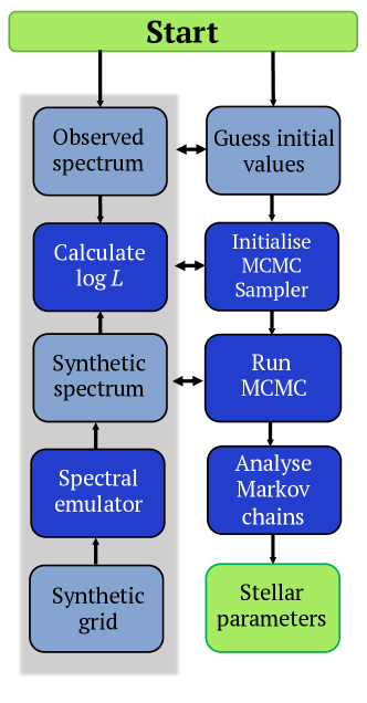
Figure 1: Diagram of the SteParSyn internal workflow.

2.2 Synthetic grid

We provide a grid of synthetic spectra with the public version of SteParSyn. We computed this grid thanks to the radiative transfer code Turbospectrum (Plez 2012). In order to generate a synthetic spectrum,Turbospectrum needs the following input data: (1) wavelength region to synthesise; (2) a model atmosphere; (3) atomic and molecular data; (4) the chemical composition of the model atmosphere. To that aim, we compiled 296 Fe i and 31 Fe ii lines from the following literature sources: Hekker & Meléndez (2007), Genovali et al. (2013), Tsantaki et al. (2014), and Tabernero et al. (2019). Using these iron lines, we produced a list of wavelength regions to synthesise. They were created to cover a 3 Å-wide region centred around each individual line (merging them when necessary, see Table 7), following the approach taken by Tsantaki et al. (2014). In addition, we chose the MARCS model atmospheres with a standard composition (Gustafsson et al. 2008) spanning from 3 500 to 7 000 K in $T_{\rm eff}$, 0.0 to 5.5 dex in $\log{g}$, and $-$2.0 to 1.0 dex in [Fe/H], whereas $\xi$ was set to the values given by the Dutra-Ferreira et al. (2016) calibration.

The atomic line data were taken from the public version of the Gaia-ESO line list (GES, see Heiter et al. 2021). The GES line list comprises Vienna Atomic Line Database (VALD3, Ryabchikova et al. 2015) data plus some highly accurate sources for the atomic parameters on top of hyperfine structure data, all of which were compiled under the framework of the GES collaboration. In addition to the atomic data, we included data for the following molecular species: CH, MgH, SiH, CaH, C₂, CN, TiO, VO, and ZrO (see Table 1). We also removed some transitions from the TiO, VO, and ZrO line lists due to their overwhelming size. Consequently, we followed the automatic recipes provided with the B. Plez molecular databases, which in turn rely on the following expression, as defined by Gray (2008):

$$\log{({gf_{i}\cdot\lambda_{i}})}-\chi_{i}\cdot\theta>-4+\max[\log{({gf_{i}\cdot\lambda_{i}})}-\chi_{i}\cdot\theta],$$ (2)

where $\log{gf}_{i}$ is the oscillator strength of a given transition, $\lambda_{i}$ is the wavelength in Å, $\chi_{l}$ is the excitation potential of the lower level in eV, and $\theta=5\,040/T$ eV^-1, with $T=3\,500$ K, and $i$ denotes transition. This approach allowed us to reduce the size of the molecular line lists and use only those transitions that significantly contribute to the spectral synthesis.

Table 1: Molecular data employed in this work.

Molecule	Reference
CH	Masseron et al. (2014)
MgH	Hinkle et al. (2013)
SiH	Kurucz (2010)
CaH	B. Plez (priv. comm., see Heiter et al. 2021)
C2	Brooke et al. (2013), Ram et al. (2014)
CN	Sneden et al. (2014)
TiO	B. Plez (priv. comm., see Heiter et al. 2021)
VO	B. Plez (priv. comm., see Heiter et al. 2021)
ZrO	B. Plez (priv. comm., see Heiter et al. 2021)

Regarding the chemical composition of the models, we assumed the solar abundances of Asplund et al. (2009) that we scaled according to the composition of each MARCS model atmosphere. In fact, the MARCS models with standard composition take into account the galactic gradient for the so-called $\alpha$-elements (i.e. O, Mg, Si, S, Ar, Ca, and Ti). In consequence, we adopted the following values of the $\alpha$-enhancement (${\rm[\alpha/Fe]}$) as function of metallicity ([Fe/H]): ${\rm[\alpha/Fe]}=0$ if ${\rm[Fe/H]}\geq 0$, ${\rm[\alpha/Fe]}=-0.4{\rm[Fe/H]}$ if $-1<{\rm[Fe/H]}<0$, and ${\rm[\alpha/Fe]}=0.4$ if ${\rm[Fe/H]}\leq-1$.

Finally, under the previous assumptions, we ran Turbospectrum to compute the synthetic spectra corresponding to the wavelength regions defined in Table 7. Then, we merged these regions into a single plain text file for each MARCS atmospheric model. These files are later stored into a binary file by means of the pickle Python library (Van Rossum 2020).

2.3 Spectral emulator

The SteParSyn code implements a likelihood function that yields the probability of a synthetic spectrum reproducing the observations (see Eq. 2). Unfortunately, the stellar atmospheric models are only available at discrete points that do not cover the whole parameter space in a continuous manner. Therefore, we need to be able to produce a synthetic spectrum corresponding to an arbitrary point of the parameter space. The former can be achieved thanks to a spectral emulator, which combines the principal component analysis (PCA, see Pearson 1901) decomposition with an interpolation method to reconstruct a synthetic spectrum corresponding to an arbitrary point of the parameter space (see, e.g. Urbaneja et al. 2008; Czekala et al. 2015). Thus, the PCA allows us to decompose each spectrum as a linear combination according to this formula:

$$F^{\rm syn}_{\lambda}=\mu_{\lambda}+\sigma_{\lambda}\sum_{i=1}^{N_{c}}w_{i}(T_{\rm eff},\log{g},{\rm[Fe/H]})\>e^{i}_{\lambda}.$$ (3)

Each synthetic spectrum ($F^{\rm syn}_{\lambda}$) can be expressed as a combination of eigenspectra ($e^{i}_{\lambda}$) and weight coefficients ($w_{i}$) that are given by the PCA. The coefficients $\mu_{\lambda}$ and $\sigma_{\lambda}$ represent a linear transformation to the synthetic spectra. These weights are only known at those points belonging to the grid. Consequently, these weights must be interpolated to produce an spectrum corresponding to an arbitrary point in the parameter space. Then, these interpolated weights can be used to reconstruct a synthetic spectrum corresponding to any point of the parameter space covered by the grid by means of Eq. 3. We implemented in the spectral emulator the PCA algorithm of the scikit-learn library (Pedregosa et al. 2011) and the multi-dimensional interpolation algorithm of the SciPy (Virtanen et al. 2020). Interestingly enough, the weights obtained using the PCA are not equally important for the reconstruction of each grid spectrum. Interestingly, the grid described in Sect. 2.2 was generated using $\approx$ 2 000 MARCS models, and only the top 350 weights were required to bring down the error budget below the 1% hallmark (see Fig. 2).

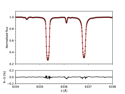
Figure 2: Top panel: Original synthetic spectrum (black line) compared to the result of the spectral emulator (shaded red line). Both spectra correspond to the following stellar parameters: $T_{\rm eff}$ $=$ 5750 K, $\log{g}$ 4.5 dex, and [Fe/H] $=$ 0.0 dex. Bottom panel: Differences between the reconstructed and original spectra (R-O).

Finally, the resulting reconstructed synthetic spectrum does not account for the macroturbulence ($\zeta$), the projected rotational velocity ($\varv\sin{i}$), and/or the instrumental resolution. These effects are taken into account by convolving, on the fly, the synthetic spectrum with a broadening kernel. Both $\zeta$ and $\varv\sin{i}$ are too degenerate in the case of FGKM-type stars and they cannot be easily disentangled from each other. One approximation is to model them by means of a single stellar rotation kernel (e.g. Gavel et al. 2019). Therefore, SteParSyn convolves the synthetic spectrum with a Gray rotation kernel (Gray 2008) to account for both $\zeta$ and $\varv\sin{i}$ followed by a Gaussian kernel with a full width at half maximum (FWHM) corresponding to the resolving power of the observations.

3 Code performance

3.1 Test sample

We gathered a sample of 35 late-type stars in order to benchmark SteParSyn. Our target list comprises 23 Gaia benchmark stars (Heiter et al. 2015a), ten late-type stars with measured interferometric angular diameters (see Boyajian et al. 2012a, b), and two well-known exoplanet host stars (HD 189733 and HD 209458, see Boyajian et al. 2015). All these targets have accurate $T_{\rm eff}$ and $\log{g}$ values determined independently from spectroscopy. According to their reported parameters, they are spread across the parameter space approximately from 3 700 K to 6 700 K in $T_{\rm eff}$, and 0.7 dex to 4.7 dex in $\log{g}$ (see Table 4). We observed them at the 1.2-m Mercator Telescope using the High Efficiency and Resolution Mercator Echelle Spectrograph (HERMES, see Raskin et al. 2011) located at the Observatorio del Roque de los Muchachos (La Palma, Spain) between 2010 and 2016 (see Table 3). The HERMES spectrograph covers a wavelength range from 3 770 to 9 000 Å with a resolving power of $R$ $=$ $85\,000$ and they were later reduced on-site by means of the HERMES automatic reduction pipeline. We note that these observations include a solar spectrum that was taken by pointing the telescope at the asteroid Vesta (see Tabernero et al. 2017).

Finally, we shifted these spectra to the laboratory reference frame by correcting for the radial velocity (RV) of the star. We derived the RVs of our targets using the method described in (Pepe et al. 2002) to compute the cross-correlation function (CCF). We sampled the CCF in the range from $-$200 to 200 km s^-1 with a step of 0.5 km s^-1, using masks that are 1 km s^-1 wide and proportionally weighted to their normalised intensity with respect to the continuum. We assigned each individual weight according to the intensities given by a VALD3 extract stellar query with parameters $T_{\rm eff}$ $=$ 5 750 K, $\log{g}$ $=$ 4.5 dex, and [Fe/H] $=$ 0.0 dex. We then fitted a Gaussian profile to each CCF to extract the corresponding RVs and calculated their uncertainties by means of the approach described in Zucker (2003) using the implementation of Blanco-Cuaresma et al. (2014). We list these RVs and their associated uncertainties in Table 3.

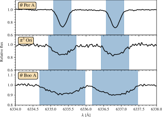
Figure 3: Line masks (shaded blue regions) around the Fe i lines at 6335.33 and 6336.82 Å for three F-type stars with different $\varv\sin{i}$ values (see text for details).

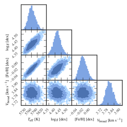
Figure 4: Posterior marginalised distributions corresponding to the following stellar parameters: $T_{\rm eff}$, $\log{g}$, [Fe/H], and $V_{\rm broad}$ for the G2 V star 18 Sco. The 1, 2, and 3 $\sigma$ levels are represented by three different colour shades.

.

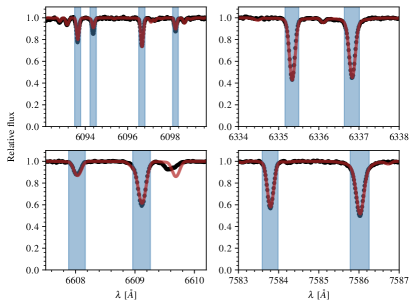
Figure 5: Four representative wavelength regions in the spectrum of 18 Sco. The shaded blue areas represent the line masks, whereas the observations are given by the black line, and the best-fitting synthetic spectrum is represented by a red line.

3.2 Stellar atmospheric parameters

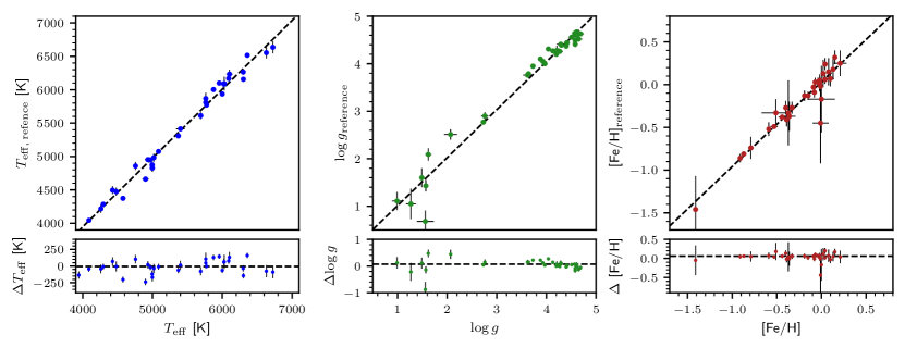
Figure 6: SteParSyn results plotted against the reference values given in Table 4. Upper panels: One-to-one correspondence. Bottom panels: Absolute differences. The dashed black lines in the upper panels correspond to a one-to-one relation, whereas in the bottom panel they correspond to zero.

We derived the stellar atmospheric parameters of our targets with SteParSyn. Thus, we employed the HERMES observations listed in Table 3, the synthetic grid described in Sect. 2.2, and a list of spectral masks generated with a custom procedure that we detail below.

The list of spectral masks was generated to cover only the Fe i and Fe ii lines in the synthetic grid. The underlying idea of deriving the atmospheric parameters using masks around iron lines is to mimic the EW method (see, e.g. Sbordone et al. 2014; Blanco-Cuaresma et al. 2014). To build the line masks, we did a Gaussian fit to our iron lines using the Levenberg–Marquardt algorithm (LMA) implemented in the Python SciPy library (Virtanen et al. 2020). In summary, our modelling provides the Gaussian parameters of the line under analysis (i.e. continuum level, centre, amplitude, depth, and $\sigma$). The fitting window is 1.5Å, and the continuum level is assumed to be modelled by a constant value. Shortly after, we removed the features whose fitted central wavelengths deviated more than 0.05 Å from their known rest-frame wavelengths. After this filter, the line masks were constructed using an iterative algorithm. We assumed an initial span for the masks of 3$\sigma$ around the centre of each line and adjusted their width to avoid including any neighbouring spectral features. The adjustment of the line masks is performed according to the quality of the Gaussian fit. To that aim, we computed the absolute value of the residuals contained with the initial interval and kept those flux points that deviated no more than 3$\sigma$ from the Gaussian fit. In other words, the initial mask size is effectively reduced until it continuously covers the line of interest and it avoids the contamination of neighbouring features. However, the Gaussian approximation is no longer valid to reproduce the weak lines when $\varv\sin{i}>15$ km s^-1. We note that only $\pi^{3}$ Ori and $\theta$ Boo A have a $\varv\sin{i}$ above the 15 km s^-1 mark. In consequence, we followed a different strategy for these two targets to build their line masks. To that aim, we gathered the lines fitted for the star $\theta$ Per A and modified them to take into account the stellar rotation. The widths of the new line masks were set to the value given by this formula: $\Delta\lambda$ $=$ $2\lambda_{\rm o}$ $\varv\sin{i}/c$, where $c$ is the speed of light in km s^-1 and $\lambda_{\rm o}$ is the centre of the line given in Å. We illustrate this procedure for two representative Fe i lines belonging to the spectra of $\theta$ Per A, $\pi^{3}$ Ori, and $\theta$ Boo A in Fig. 3.

After we computed the line masks corresponding to our selected Fe i,ii lines, we turned to the broadening parameters of our targets. The SteParSyn code models the total line broadening with two components. The first component ($V_{\rm broad}$) accounts for the broadening parameters $\zeta$ and $\varv\sin{i}$. We chose to model both of them with a single rotation kernel following the prescription given by Gavel et al. (2019). The second component corresponds to the instrumental line spread function (LSF) that we described with a Gaussian function corresponding to the HERMES resolving power (i.e. $R$ $=$ 85 000). The quantity $V_{\rm broad}$ was derived only for those stars with significant broadening parameters. In fact, when $V_{\rm broad}$ is small enough, the total line broadening is entirely dominated by the LSF of the instrument (Reiners et al. 2018). This affects some mid-to-late K dwarf stars in our sample with reported $\varv\sin{i}$ values on or below the noise-driven limit of 2 km s^-1 (Gray 2008). Moreover, they are expected to have small macroturbulent velocities (see Brewer et al. 2016) that translate into an LSF-dominated line broadening. Consequently, we fixed the $V_{\rm broad}$ of those K-stars to the $\varv\sin{i}$ reported in the literature (see Table 4). Then, we ran SteParSyn and calculated the stellar atmospheric parameters for our targets. We list the stellar parameters calculated with SteParSyn in Table 5. We also represent the marginalised results provided by SteParSyn for the G2 V star 18 Sco in Fig. 4 and the best fit to some representative iron lines in Fig. 5.

We then compared our results to the reference parameters (see Table 4) and represented them in Fig. 6. Then, following Tabernero et al. (2019), we performed 10 000 Monte Carlo simulations on our data in the hope of assessing possible sources of tentatively systematic offsets. We found the following differences with the reference parameters: $-$12 $\pm$ 117 K in $T_{\rm eff}$, 0.04 $\pm$ 0.14 dex in $\log{g}$, and 0.05 $\pm$ 0.09 dex in [Fe/H]. These differences show that SteParSyn can reproduce the reference values for our sample stars since they are compatible with zero in all instances. In parallel, we populated a Kiel diagram (see Fig. 7) with our $T_{\rm eff}$ and $\log{g}$ values alongside the PARSEC isochrones (Bressan et al. 2012). The isochrones we represent in the Kiel diagram encompass our points and they are well-behaved even for the coolest stars in the main-sequence, contrary to what has been found in previous works (see Mortier et al. 2014; Montes et al. 2018; Tsantaki et al. 2019; Brucalassi et al. 2021). Finally, we compared our $V_{\rm broad}$ values to those of other late-type stars. Thus, we gathered the broadening values calculated by Brewer et al. (2016) and represented them against our own as a function of $T_{\rm eff}$ in Fig. 8. From this comparison, we see that our calculated $V_{\rm broad}$ values follow the behaviour of the literature values for other late-type stars reported in (Brewer et al. 2016).

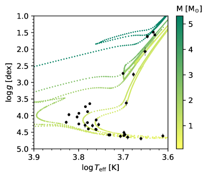
Figure 7: Kiel diagram ($\log{g}$ vs. $\log{T_{\rm eff}}$) for all the spectra analysed alongside the PARSEC isochrones for 0.1, 0.5, 1, 5, and 10 Ga for solar metallicity (Bressan et al. 2012).

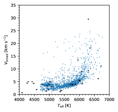
Figure 8: Comparison of the $V_{\rm broad}$ derived in this work represented by black circles and the values derived by Brewer et al. (2016) are displayed with blue circles.

3.3 Trigonometric gravities, radii, and masses

The surface gravities derived with spectroscopic data are sometimes not entirely in agreement with those calculated using evolutionary models, visual magnitudes, and parallaxes (Tsantaki et al. 2019; Brucalassi et al. 2021). The use of evolutionary models provides us with an alternative method that can be used to assess the precision of the spectroscopic $\log{g}$ values. For these reasons, we used the PARAM web interface (da Silva et al. 2006) alongside the $T_{\rm eff}$ and [Fe/H] inferred with SteParSyn, the Gaia EDR3 (Gaia Collaboration et al. 2021) or Hipparcos (van Leeuwen 2007) parallax and their visual magnitude ($V$), and the PARSEC stellar evolutionary tracks and isochrones (Bressan et al. 2012). From this information, we calculated the so-called trigonometric surface gravity ($\log{g_{\rm trig}}$), mass ($M_{*}$), and radius ($R_{*}$) for our targets (see Table 5). We compare the spectroscopic gravities derived with SteParSyn against their trigonometric counterparts in Fig. 9. Again, we ran 10 000 MC simulations and computed a mean difference of -0.03 $\pm$ 0.11 dex, which is in turn compatible with zero at the 1$\sigma$ level. This difference implies that our spectroscopic surface gravities are fully consistent with the PARAM trigonometric values at the 0.1 dex mark.

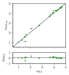
Figure 9: SteParSyn -based surface gravities plotted against the trigonometric values based on the parallaxes listed in Table 5.

3.4 SteParSyn vs. StePar

The analysis described in this work uses a selection of Fe i and Fe ii lines to derive the stellar parameters of our sample stars. In ideal terms, the synthetic method should deliver the same stellar parameters as the EW method. To quantify the former statement, we calculated the stellar parameters for those targets that can be analysed under the EW method with the StePar code. To that aim, we selected the stars of our sample with $\varv\sin{i}$ $<$ 15 km s^-1 and spectral types between F6 and K4 (see Tabernero et al. 2019). Using these criteria, we finished with a sub-sample of 28 stars. Shortly after, we used the ARES (version 2, see Sousa et al. 2015) code to measure the EW of the Fe lines listed listed in Table 7 for these stars. We calculated the stellar parameters for this sub-sample with StePar (see Table 6). We then compared the results of SteParSyn and StePar. Thus, we retrieve the following differences between them: 40 $\pm$ 87 K for $T_{\rm eff}$, $-$0.04 $\pm$ 0.21 dex for $\log{g}$, and 0.04 $\pm$ 0.08 dex for [Fe/H]. These differences are compatible within the error bars. Therefore, StePar and SteParSyn deliver compatible results when we analyse the same observational data. Regarding the uncertainties on the parameters, StePar gives the following average values: $\Delta$ $T_{\rm eff}$ $=$ 50 K, $\Delta$ $\log{g}$ $=$ 0.13 dex and $\Delta$ [Fe/H] $=$ 0.04 dex; whereas, for SteParSyn we find 29 K, 0.06 dex, and 0.03 dex. Thus, the SteParSyn uncertainties are smaller by a factor 2 for $T_{\rm eff}$ and $\log{g}$, whereas both codes provide similar errors on [Fe/H].

4 Discussion

The stellar atmospheric parameters obtained with SteParSyn for our target stars are reliable down to the 1$\sigma$ level with the reference parameters (Table 4), the trigonometric gravities of Table 5, and the parameters provided by the EW method implemented in StePar (see Table 6). Roughly speaking, these differences are at the level of 100 K for $T_{\rm eff}$, 0.1 dex for $\log{g}$, and 0.1 dex for [Fe/H] (see Table 2). However, these average differences alone are not enough to explore hidden systematic uncertainties tied to the SteParSyn stellar parameters. Thus, we calculated the correlation between the individual differences against the parameters themselves following the approach described in Tabernero et al. (2019). We performed 10 000 Monte Carlo (MC) simulations on our data to compute both Pearson and Spearman correlation coefficients ($r_{p}$ and $r_{s}$, respectively) and their uncertainties. We provide the results of these MC simulations in Table 2. These simulations reveal that the correlation between differences and a given parameter are small. Consequently, the average differences found for the stellar atmospheric only correspond to systematic uncertainties intrinsic to the SteParSyn code.

We notice that SteParSyn [Fe/H] values for both $\alpha$ Cet and $\gamma$ Sge are not entirely in agreement with reference parameters. However, their reference [Fe/H] values largely have error bars at the level of 0.4–0.5 dex, and they are not well-constrained. A similar argument applies to the surface gravities of some giant stars. Moreover, reproducing the surface gravities of the giant stars is by no means an easy task. Stars such as $\mu$ Leo, $\alpha$ Cet, and HD 107328 have surface gravities that are uncertain for a number of currently known reasons. In fact, according to Heiter et al. (2015b) their masses have large uncertainties ranging from approximately 0.5 to 1.0 $M_{\odot}$ that translate into surface gravities that are not well-defined. In spite of those uncertain $\log{g}$ values, SteParSyn manages to produce reliable parameters for our target stars. In addition, their $T_{\rm eff}$ and $\log{g}$ values are in agreement with evolutionary models in the Kiel diagram (see Fig. 7). These findings are reinforced by the fact that SteParSyn produces values of $V_{\rm broad}$ consistent with the behaviour of those calculated by Brewer et al. (2016), as we show in Fig.8.

Finally, we want to address the limitations of the SterParSyn code regarding the analysis of late-type spectra under the spectral synthesis method. First, the observational data must be of high enough quality to be analysed. This means that, since low signal-to-noise ratios (S/N) translate into higher uncertainties on the stellar atmospheric parameters (Smiljanic et al. 2014). To compute the performance of SteParSyn at different S/N, we took the spectra of 18 Sco and $\epsilon$ Eri and we degraded them to the following S/N values: 10, 20, 30, 40, 50, 80, and 100. Then, we ran SteParSyn in order to calculate the stellar parameters of the degraded spectra. According to these calculations, the parameters have uncertainties at the level of 100 K for $T_{\rm eff}$, 0.2 dex for $\log{g}$, and 0.1 dex for [Fe/H] at S/N $=$ 20. (see Fig. 10). In addition, at S/N $=$ 10 the errors on the stellar parameters reach the level of 200 K, 0.5 dex, and 0.2 dex. In light of these numbers, the stellar parameters become unreliable for those spectra with S/N $<$ 20. Second, SteParSyn cannot analyse double-lined spectra because it is not capable of disentangling two or more stellar components. A third limitation is the $\varv\sin{i}$ of the star under analysis. The fastest rotator in our sample is $\theta$ Boo A with a $\varv\sin{i}$ of $\approx$ 30 km s^-1 and we were able to calculate its stellar parameters with SteParSyn. Therefore, the limit on $\varv\sin{i}$ for the code should be above 30 km s^-1. In fact, the limit on $\varv\sin{i}$ is related to the size of the spectral regions under analysis (Tsantaki et al. 2014). In general terms, the stellar rotation dilutes the spectral lines producing both narrow, broad, and likely blended spectral features. The line dilution should translate into less reliable stellar parameters, which we should be able to quantify. To that aim, we broadened the spectra of the stars 18 Sco and $\epsilon$ Eri by means of the Gray rotation kernel (Gray 2008) to different $\varv\sin{i}$ values. We chose these $\varv\sin{i}$ values to be in the 10–50 km s^-1 range, taking a step of 5 km s^-1. Thus, we calculated the stellar parameters of these rotationally-broadened spectra with SteParSyn. Then, we compared this value to the parameters obtained for the original unbroadened spectra of both 18 Sco and $\epsilon$ Eri. We represent these differences as functions of $\varv\sin{i}$ in Fig. 10. In all, SteParSyn can recover the stellar parameters up to $\varv\sin{i}$ $=$ 30 km s^-1 with differences of no more than 50 K, 0.1 dex, and 0.05 dex for $T_{\rm eff}$, $\log{g}$, and [Fe/H], respectively. However, SteParSyn does not recover the expected stellar parameters for $\varv\sin{i}$ $\geq$ 35 km s^-1.

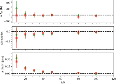
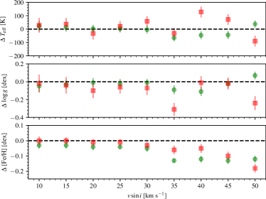
Figure 10: Variation of the stellar atmospheric parameters as a function of S/N (top panel) and $\varv\sin{i}$ (bottom panel). The values corresponding to 18 Sco (G2 V) are represented by green circles, whereas those corresponding to $\epsilon$ Eri (K2 V) are displayed as red squares (see text for details).

Table 2: Summary of the MC simulations on $T_{\rm eff}$, $\log{g}$, and [Fe/H] calculated with SteParSyn against three samples of stellar parameters: literature values, StePar, and the trigonometric surface gravities derived using PARAM. We provide differences on each parameter alongside the Pearson ($r_{p}$) and the Spearman ($r_{s}$) correlation coefficients (see text for details).

Sample	Parameter	Difference	$r_{p}$	$r_{s}$
	$T_{\rm eff}$	$-$12 $\pm$ 117 K	0.19 $\pm$ 0.10	0.21 $\pm$ 0.10
Literature	$\log{g}$	0.04 $\pm$ 0.14 dex	$-$0.34 $\pm$ 0.11	0.04 $\pm$ 0.14
	$[$Fe/H$]$	0.05 $\pm$ 0.09 dex	$-$0.04 $\pm$ 0.16	$-$0.05 $\pm$ 0.16
	$T_{\rm eff}$	40 $\pm$ 87 K	0.07 $\pm$ 0.12	0.06 $\pm$ 0.13
StePar	$\log{g}$	$-$0.04 $\pm$ 0.21 dex	$-$0.51 $\pm$ 0.13	$-$ 0.41 $\pm$ 0.12
	$[$Fe/H$]$	0.04 $\pm$ 0.08 dex	0.28 $\pm$ 0.12	0.21 $\pm$ 0.11
	$T_{\rm eff}$	—	—	—
PARAMa	$\log{g}$	$-$0.03 $\pm$ 0.11 dex	$-$0.12 $\pm$ 0.12	0.24 $\pm$ 0.12
	$[$Fe/H$]$	—	—	—

5 Conclusions

In this work, we provide a description of the SteParSyn code. The code is designed to infer the atmospheric parameters ($T_{\rm eff}$, $\log{g}$, [Fe/H], and $V_{\rm broad}$) of FGKM-type stars under the spectral synthesis method. The SteParSyn code is publicly available to the community in a GitHub repository. In summary, it relies on the MCMC sampler emcee in conjunction with an spectral emulator that can interpolate spectra down to a precision $<$ 1%. We also provide a grid of synthetic spectra with the code that allow the user to characterise the spectra of FGKM-type stars with parameters in the range of 3 500 to 7 000 K in $T_{\rm eff}$, 0.0 to 5.5 dex in $\log{g}$, and $-$2.0 to 1.0 dex in [Fe/H].

We tested the performance of the code against a sample of well-known 35 FGKM-type stars observed with the HERMES spectrograph. We found that SteParSyn infers stellar parameters that are consistent with the reference values. In addition, the $\log{g}$ values inferred with SteParSyn are compatible with the trigonometric surface gravities provided by PARAM down to the 0.1 dex mark. Furthermore, we found good agreement between the results provided by both SteParSyn and StePar.

Finally, we want to note the limitations of the synthetic method that should be taken into consideration when using SteParSyn. First, the spectroscopic data must have an S/N $\geq$ 20. Second, the code is meant to analyse only single-lined spectra as it cannot disentangle the flux of two or more stellar components. Third, the implementation of the spectral synthesis method provided in this work can only give reliable parameters for stars with $\varv\sin{i}$ on or below the 30 km s^-1 mark.

Appendix A Extra material

The sample analysed in this work is given in Table 3, whereas Table 4 contains the reference stellar atmospheric parameters compiled from literature sources. The stellar parameters of those stars analysed with SteParSyn are given in Table 5, whereas Table 6 contains the StePar parameters. Finally, the wavelength regions containing the Fe i,ii lines studied in this work are given in Table 7.

Table 3: Names, coordinates, visual magnitudes ($V$), spectral types (SpT), signal-to-noise ratios (S/N), radial velocities (RV), and parallaxes ($\pi$) for the stars analysed in this work. The parallaxes were collected from the Gaia EDR3 (Gaia Collaboration et al. 2021) unless stated otherwise.

Name	HIP	$\alpha$ (J2000)	$\delta$ (J2000)	$V$	SpT	S/Na	RV	$\pi$
				[mag]			[km s-1]	[mas]
Sun (Vesta)	…	…	…	…	G2 V	139	…	…
HD 4628	3765	00:48:22.98	+05:16:50.21	5.74	K2 V	122	$-$9.997 $\pm$ 0.010	134.50 $\pm$ 0.058
$\eta$ Cas A	3821	00:49:06.29	+57:48:54.67	3.44	G0 V	268	8.547 $\pm$ 0.015	168.83 $\pm$ 0.17
$\mu$ Cas	5336	01:08:16.40	+54:55:13.23	5.17	G5 Vb	194	$-$96.540 $\pm$ 0.015	130.29 $\pm$ 0.44
$\tau$ Cet	8102	01:44:04.08	$-$15:56:14.93	3.50	G8.5 V	194	$-$16.530 $\pm$ 0.011	273.81 $\pm$ 0.17
HD 16160	12114	02:36:04.90	+06:53:12.43	5.83	K3 V	187	25.763 $\pm$ 0.009	138.34 $\pm$ 0.32
$\theta$ Per A	12777	02:44:11.99	+49:13:42.41	4.11	F7 V	250	24.620 $\pm$ 0.028	89.69 $\pm$ 0.16
$\alpha$ Cet	14135	03:02:16.77	+04:05:23.06	2.53	M1.5 IIIa	117	$-$25.784 $\pm$ 0.011	13.09 $\pm$ 0.44
$\epsilon$ Eri	16537	03:32:55.85	$-$09:27:29.73	3.73	K2 V	208	16.449 $\pm$ 0.010	310.58 $\pm$ 0.14
HD 22879	17147	03:40:22.07	$-$03:13:01.13	6.67	F9 V	112	120.475 $\pm$ 0.023	38.325 $\pm$ 0.031
$\delta$ Eri	17378	03:43:14.90	$-$09:45:48.21	3.54	K1 III-IV	190	$-$6.155 $\pm$ 0.008	110.03 $\pm$ 0.19
Aldebaran	21421	04:35:55.24	+16:30:33.49	0.86	K5 III	151	54.120 $\pm$ 0.009	47.253 $\pm$ 0.096
$\pi^{3}$ Ori	22449	04:49:50.41	+06:57:40.59	3.19	F6 V	93	25.074 $\pm$ 0.070	124.62 $\pm$ 0.23
HD 49933	32851	06:50:49.83	$-$00:32:27.18	5.77	F2 V	130	$-$12.275 $\pm$ 0.054	33.534 $\pm$ 0.043
Procyon	37279	07:39:18.12	+05:13:29.96	0.37	F5 IV-V	432	$-$5.275 $\pm$ 0.023	284.56 $\pm$ 1.26b
$\beta$ Gem	37826	07:45:18.95	+28:01:34.32	1.14	K0 IIIb	183	3.536 $\pm$ 0.007	96.54 $\pm$ 0.27b
$\mu$ Leo	48455	09:52:45.82	+26:00:25.03	3.88	K2 III	112	13.764 $\pm$ 0.007	26.10 $\pm$ 0.20
20 LMi	49081	10:01:00.66	+31:55:25.22	5.40	G3 V	224	56.118 $\pm$ 0.010	66.996 $\pm$ 0.092
36 UMa	51459	10:30:37.58	+55:58:49.94	4.72	F8 V	193	8.880 $\pm$ 0.016	77.249 $\pm$ 0.081
$\beta$ Vir	57757	11:50:41.72	+01:45:52.99	3.60	F9 V	152	4.757 $\pm$ 0.014	90.90 $\pm$ 0.19
Gmb 1830	57939	11:52:58.77	+37:43:07.24	6.45	G8 Vp	205	$-$98.001 $\pm$ 0.022	109.030 $\pm$ 0.020
HD 107328	60172	12:20:20.98	+03:18:45.26	4.96	K0 IIIb	145	36.656 $\pm$ 0.009	9.67 $\pm$ 0.15
$\epsilon$ Vir	63608	13:02:10.60	+10:57:32.94	2.79	G8 III	204	$-$14.169 $\pm$ 0.009	30.21 $\pm$ 0.19
$\beta$ Com	64394	13:11:52.39	+27:52:41.45	4.25	G0 V	231	5.438 $\pm$ 0.016	108.73 $\pm$ 0.17
$\eta$ Boo	67927	13:54:41.08	+18:23:51.80	2.68	G0 IV	258	7.109 $\pm$ 0.028	87.75 $\pm$ 1.24b
Arcturus	69673	14:15:39.67	+19:10:56.67	$-$0.05	K1.5 III	207	$-$4.880 $\pm$ 0.009	88.83 $\pm$ 0.54b
$\theta$ Boo A	70497	14:25:11.80	+51:51:02.68	4.05	F7 V	223	$-$10.734 $\pm$ 0.117	69.07 $\pm$ 0.16
18 Sco	79672	16:15:37.27	$-$08:22:09.98	5.50	G2 Va	202	12.000 $\pm$ 0.011	70.737 $\pm$ 0.063
$\gamma$ Sge	98337	19:58:45.43	+19:29:31.73	3.47	M0 III	127	$-$33.712 $\pm$ 0.008	13.09 $\pm$ 0.44
HD 189733	98505	20:00:43.71	+22:42:39.07	7.65	K2 V	153	$-$1.925 $\pm$ 0.011	50.567 $\pm$ 0.016
61 Cyg A	104214	21:06:53.94	+38:44:57.90	5.21	K5 V	138	$-$65.562 $\pm$ 0.013	285.995 $\pm$ 0.060
61 Cyg B	104217	21:06:55.26	+38:44:31.36	6.03	K7 V	115	$-$64.232 $\pm$ 0.019	286.005 $\pm$ 0.029
HD 209458	108859	22:03:10.77	+18:53:03.55	7.63	F9 V	167	$-$14.678 $\pm$ 0.017	20.769 $\pm$ 0.027
$\xi$ Peg	112447	22:46:41.58	+12:10:22.39	4.20	F7 V	296	$-$5.841 $\pm$ 0.030	60.92 $\pm$ 0.17
HD 220009	115227	23:20:20.58	+05:22:52.70	5.07	K2 III	213	40.793 $\pm$ 0.009	9.09 $\pm$ 0.12

Table 4: Reference stellar atmospheric parameters for the stars analysed in this work.

Name	SpT	$T_{\rm eff}$	$\log{g}$	Ref.a	[Fe/H]	Ref.b	$\varv\sin{i}$	Ref.c
		[K]	[dex]		[dex]		[km s-1]
Sun	G2 V	5771 $\pm$ 1	4.44 $\pm$ 0.01	Hei15	0.03 $\pm$ 0.05	Jof14	1.6	Vf05
HD 4628	K2 V	4950 $\pm$ 14	4.64 $\pm$ 0.01	Boy12bd	$-$0.27 $\pm$ 0.04	Pastel	2.0	Mar14
$\eta$ Cas A	G0 V	6003 $\pm$ 24	4.39 $\pm$ 0.01	Boy12ad	$-$0.27 $\pm$ 0.07	Pastel	5.4	Luc17
$\mu$ Cas	G5 Vb	5308 $\pm$ 29	4.41 $\pm$ 0.06	Hei15	$-$0.81 $\pm$ 0.03	Jof14	1.1	Hal94
$\tau$ Cet	G8.5 V	5414 $\pm$ 21	4.49 $\pm$ 0.03	Hei15	$-$0.49 $\pm$ 0.03	Jof14	1.6	Jen11
HD 16160	K3 V	4662 $\pm$ 17	4.52 $\pm$ 0.01	Boy12bd	$-$0.13 $\pm$ 0.06	Pastel	1.3	Que98
$\theta$ Per A	F7 V	6157 $\pm$ 37	4.26 $\pm$ 0.01	Boy12ad	0.00 $\pm$ 0.08	Pastel	10.2	Luc17
$\alpha$ Cet	M1.5 IIIa	3796 $\pm$ 65	0.68 $\pm$ 0.23	Hei15	$-$0.45 $\pm$ 0.47	Jof14	6.9	Mas08
$\epsilon$ Eri	K2 V	5076 $\pm$ 30	4.61 $\pm$ 0.03	Hei15	$-$0.09 $\pm$ 0.06	Jof14	6.2	Bud19
HD 22879	F9 V	5868 $\pm$ 89	4.27 $\pm$ 0.04	Hei15	$-$0.86 $\pm$ 0.05	Jof14	4.2	Bud19
$\delta$ Eri	K1 III-IV	4954 $\pm$ 30	3.76 $\pm$ 0.02	Hei15	0.06 $\pm$ 0.05	Jof14	3.2	Sot18
Aldebaran	K5 III	3927 $\pm$ 40	1.11 $\pm$ 0.19	Hei15	$-$0.37 $\pm$ 0.17	Jof14	4.3	Mas08
$\pi^{3}$ Ori	F6 V	6516 $\pm$ 19	4.31 $\pm$ 0.01	Boy12ad	0.05 $\pm$ 0.07	Pastel	18.5	Luc17
HD 49933	F2 V	6635 $\pm$ 91	4.20 $\pm$ 0.03	Hei15	$-$0.41 $\pm$ 0.08	Jof14	5.0	Tak05
Procyon	F5 IV-V	6554 $\pm$ 84	4.00 $\pm$ 0.02	Hei15	0.01 $\pm$ 0.08	Jof14	7.4	Luc17
$\beta$ Gem	K0 IIIb	4858 $\pm$ 60	2.90 $\pm$ 0.08	Hei15	0.13 $\pm$ 0.16	Jof14	2.8	Mas08
$\mu$ Leo	K2 III	4474 $\pm$ 60	2.51 $\pm$ 0.11	Hei15	0.25 $\pm$ 0.15	Jof14	4.5	Mas08
20 LMi	G3 V	5612 $\pm$ 52	4.26 $\pm$ 0.03	Boy12ad	0.18 $\pm$ 0.12	Pastel	4.7	Luc17
36 UMa	F8 V	6233 $\pm$ 68	4.41 $\pm$ 0.03	Boy12ad	$-$0.13 $\pm$ 0.05	Pastel	5.3	Luc17
$\beta$ Vir	F9 V	6083 $\pm$ 41	4.10 $\pm$ 0.02	Hei15	0.24 $\pm$ 0.07	Jof14	6.4	Luc17
Gmb 1830	G8 Vp	4827 $\pm$ 55	4.60 $\pm$ 0.03	Hei15	$-$1.46 $\pm$ 0.39	Jof14	0.0	Lat02
HD107328	K0 IIIb	4496 $\pm$ 59	2.09 $\pm$ 0.13	Hei15	$-$0.33 $\pm$ 0.16	Jof14	1.9	Mas08
$\epsilon$ Vir	G8 III	4983 $\pm$ 61	2.77 $\pm$ 0.02	Hei15	0.15 $\pm$ 0.16	Jof14	1.4	Jof15
$\beta$ Com	G0 V	5936 $\pm$ 33	4.37 $\pm$ 0.01	Boy12ad	0.07 $\pm$ 0.09	Pastel	6.6	Luc17
$\eta$ Boo	G0 IV	6099 $\pm$ 28	3.79 $\pm$ 0.02	Hei15	0.32 $\pm$ 0.08	Jof14	14.4	Luc17
Arcturus	K1.5 III	4286 $\pm$ 35	1.60 $\pm$ 0.20	Hei15	$-$0.52 $\pm$ 0.08	Jof14	4.2	Mas08
$\theta$ Boo A	F7 V	6265 $\pm$ 41	4.05 $\pm$ 0.04	Boy12ad	$-$0.03 $\pm$ 0.03	Pastel	30.4	Luc17
18 Sco	G2 Va	5810 $\pm$ 80	4.44 $\pm$ 0.03	Hei15	0.03 $\pm$ 0.03	Jof14	4.4	Luc17
$\gamma$ Sge	M0 III	3807 $\pm$ 49	1.05 $\pm$ 0.32	Hei15	$-$0.17 $\pm$ 0.39	Jof14	5.8	Mas08
HD 189733	K2 V	4875 $\pm$ 43	4.56 $\pm$ 0.03	Boy15d	$-$0.02 $\pm$ 0.04	Pastel	4.5	Luc17
61 Cyg A	K5 V	4374 $\pm$ 22	4.63 $\pm$ 0.04	Hei15	$-$0.33 $\pm$ 0.38	Jof14	1.9	Que98
61 Cyg B	K7 V	4044 $\pm$ 32	4.67 $\pm$ 0.04	Hei15	$-$0.38 $\pm$ 0.03	Jof14	0.7	Que98
HD 209458	F9 V	6092 $\pm$ 103	4.28 $\pm$ 0.10	Boy15d	0.03 $\pm$ 0.05	Pastel	3.9	Sot18
$\xi$ Peg	F7 V	6168 $\pm$ 36	3.95 $\pm$ 0.01	Boy12ad	$-$0.27 $\pm$ 0.08	Pastel	9.7	Luc17
HD 220009	K2 III	4217 $\pm$ 60	1.43 $\pm$ 0.12	Hei15	$-$0.74 $\pm$ 0.13	Jof14	1.2	Med99

Table 5: Stellar atmospheric parameters derived with SteParSyn ($T_{\rm eff}$, $\log{g}$, [Fe/H], and $V_{\rm broad}$), trigonometric gravities ($\log{g_{\rm trig}}$), mass ($M_{*}$), and radius ($R_{*}$) for the stars analysed in this work.

Name	$T_{\rm eff}$	$\log{g}$	[Fe/H]	$V_{\rm broad}$	$\log{g_{\rm trig}}$	$M_{*}$	$R_{*}$
	[K]	[dex]	[dex]	[km s-1]	[dex]	[$M_{\odot}$]	[$R_{\odot}$]
Sun	5775 $\pm$ 13	4.41 $\pm$ 0.02	$-$0.04 $\pm$ 0.01	3.71 $\pm$ 0.03	…	1	1
HD 4628	4969 $\pm$ 37	4.57 $\pm$ 0.05	$-$0.33 $\pm$ 0.02	2a	4.59 $\pm$ 0.02	0.720 $\pm$ 0.014	0.691 $\pm$ 0.007
$\eta$ Cas A	5874 $\pm$ 34	4.30 $\pm$ 0.06	$-$0.33 $\pm$ 0.02	4.00 $\pm$ 0.07	4.30 $\pm$ 0.02	0.881 $\pm$ 0.014	1.062 $\pm$ 0.022
$\mu$ Cas	5370 $\pm$ 35	4.58 $\pm$ 0.05	$-$0.87 $\pm$ 0.02	1.1a	4.50 $\pm$ 0.01	0.747 $\pm$0.008	0.781 $\pm$ 0.018
$\tau$ Cet	5400 $\pm$ 60	4.58 $\pm$ 0.05	$-$0.53 $\pm$ 0.04	1.6a	4.54 $\pm$ 0.02	0.760 $\pm$ 0.017	0.750 $\pm$ 0.015
HD 16160	4900 $\pm$ 45	4.65 $\pm$ 0.07	$-$0.19 $\pm$ 0.02	1.3a	4.60 $\pm$ 0.02	0.741 $\pm$ 0.015	0.691 $\pm$ 0.006
$\theta$ Per A	6302 $\pm$ 20	4.25 $\pm$ 0.03	$-$0.02 $\pm$ 0.01	9.39 $\pm$ 0.04	4.30 $\pm$ 0.01	1.201 $\pm$ 0.010	1.250 $\pm$ 0.020
$\alpha$ Cet	3883 $\pm$ 41	1.56 $\pm$ 0.17	$-$0.01 $\pm$ 0.09	6.30 $\pm$ 0.23	1.08 $\pm$ 0.06	2.803 $\pm$ 0.219	77.347 $\pm$ 5.120
$\epsilon$ Eri	5086 $\pm$ 33	4.62 $\pm$ 0.06	$-$0.08 $\pm$ 0.02	3.11 $\pm$ 0.14	4.58 $\pm$ 0.02	0.806 $\pm$ 0.019	0.734 $\pm$ 0.015
HD 22879	5763 $\pm$ 30	4.13 $\pm$ 0.05	$-$0.91 $\pm$ 0.02	3.97 $\pm$ 0.08	4.29 $\pm$ 0.01	0.977 $\pm$ 0.015	1.135 $\pm$ 0.023
$\delta$ Eri	4934 $\pm$ 41	3.62 $\pm$ 0.09	0.04 $\pm$ 0.02	3.27 $\pm$ 0.11	3.67 $\pm$ 0.04	1.094 $\pm$ 0.047	2.450 $\pm$ 0.070
Aldebaran	3858 $\pm$ 21	0.99 $\pm$ 0.10	$-$0.36 $\pm$ 0.07	4.93 $\pm$ 0.13	1.02 $\pm$ 0.04	0.912 $\pm$ 0.063	47.535 $\pm$ 1.427
$\pi^{3}$ Ori	6358 $\pm$ 34	4.04 $\pm$ 0.08	$-$0.02 $\pm$ 0.02	18.20 $\pm$ 0.14	4.25 $\pm$ 0.01	1.230 $\pm$ 0.012	1.339 $\pm$ 0.029
HD 49933	6725 $\pm$ 26	4.20 $\pm$ 0.05	$-$0.39 $\pm$ 0.02	11.10 $\pm$ 0.08	4.21 $\pm$ 0.01	1.188 $\pm$ 0.014	1.379 $\pm$ 0.009
Procyon	6631 $\pm$ 34	3.97 $\pm$ 0.05	$-$0.02 $\pm$ 0.02	6.18 $\pm$ 0.03	4.00 $\pm$ 0.01	1.480 $\pm$ 0.010	1.965 $\pm$ 0.043
$\beta$ Gem	4756 $\pm$ 23	2.76 $\pm$ 0.07	0.02 $\pm$ 0.03	4.08 $\pm$ 0.07	2.73 $\pm$ 0.03	1.819 $\pm$ 0.075	9.324 $\pm$ 0.215
$\mu$ Leo	4480 $\pm$ 43	2.07 $\pm$ 0.13	0.21 $\pm$ 0.07	4.32 $\pm$ 0.12	2.41 $\pm$ 0.07	1.311 $\pm$ 0.161	11.503 $\pm$ 0.360
20 LMi	5691 $\pm$ 32	4.27 $\pm$ 0.06	0.13 $\pm$ 0.02	4.04 $\pm$ 0.07	4.29 $\pm$ 0.02	1.010 $\pm$ 0.016	1.158 $\pm$ 0.021
36 UMa	6102 $\pm$ 43	4.29 $\pm$ 0.08	$-$0.15 $\pm$ 0.03	4.19 $\pm$ 0.09	4.29 $\pm$ 0.02	1.049 $\pm$ 0.021	1.180 $\pm$ 0.027
$\beta$ Vir	6024 $\pm$ 28	3.88 $\pm$ 0.04	0.04 $\pm$ 0.02	5.24 $\pm$ 0.05	4.03 $\pm$ 0.02	1.226 $\pm$ 0.041	1.722 $\pm$ 0.032
Gmb 1830	4997 $\pm$ 18	4.60 $\pm$ 0.03	$-$1.41 $\pm$ 0.02	0a	4.60 $\pm$ 0.01	0.616 $\pm$ 0.001	0.631 $\pm$ 0.003
HD 107328	4427 $\pm$ 20	1.62 $\pm$ 0.06	$-$0.51 $\pm$ 0.16	5.00 $\pm$ 0.07	1.81 $\pm$ 0.08	1.049 $\pm$ 0.180	20.428 $\pm$ 0.540
$\epsilon$ Vir	5019 $\pm$ 23	2.73 $\pm$ 0.05	0.08 $\pm$ 0.03	5.16 $\pm$ 0.06	2.72 $\pm$ 0.01	2.878 $\pm$ 0.020	11.939 $\pm$ 0.206
$\beta$ Com	6000 $\pm$ 22	4.40 $\pm$ 0.04	0.10 $\pm$ 0.04	5.56 $\pm$ 0.05	4.40 $\pm$ 0.02	1.130 $\pm$ 0.024	1.075 $\pm$ 0.025
$\eta$ Boo	5956 $\pm$ 18	3.64 $\pm$ 0.04	0.15 $\pm$ 0.01	13.55 $\pm$ 0.05	3.73 $\pm$ 0.01	1.587 $\pm$ 0.022	2.762 $\pm$ 0.042
Arcturus	4294 $\pm$ 24	1.49 $\pm$ 0.04	$-$0.59 $\pm$ 0.02	4.98 $\pm$ 0.07	1.58 $\pm$ 0.04	0.887 $\pm$ 0.043	24.457 $\pm$ 0.606
$\theta$ Boo A	6300 $\pm$ 23	3.93 $\pm$ 0.04	$-$0.09 $\pm$ 0.01	29.50 $\pm$ 0.12	4.06 $\pm$ 0.01	1.255 $\pm$ 0.039	1.661 $\pm$ 0.010
18 Sco	5763 $\pm$ 18	4.42 $\pm$ 0.03	-0.02 $\pm$ 0.01	3.80 $\pm$ 0.03	4.39 $\pm$ 0.02	0.977 $\pm$ 0.012	1.017 $\pm$ 0.023
$\gamma$ Sge	3943 $\pm$ 25	1.27 $\pm$ 0.10	0.00 $\pm$ 0.15	5.35 $\pm$ 0.14	1.23 $\pm$ 0.08	1.446 $\pm$ 0.263	46.623 $\pm$ 2.241
HD 189733	4995 $\pm$ 32	4.51 $\pm$ 0.06	$-$0.01 $\pm$ 0.01	4.08 $\pm$ 0.09	4.55 $\pm$ 0.02	0.800 $\pm$ 0.018	0.758 $\pm$ 0.003
61 Cyg A	4576 $\pm$ 36	4.69 $\pm$ 0.06	$-$0.37 $\pm$ 0.02	1.9a	4.69 $\pm$ 0.02	0.624 $\pm$ 0.010	0.574 $\pm$ 0.005
61 Cyg B	4088 $\pm$ 26	4.61 $\pm$ 0.07	$-$0.44 $\pm$ 0.04	0.7a	4.57 $\pm$ 0.04	0.451 $\pm$ 0.024	0.562 $\pm$ 0.015
HD 209458	6028 $\pm$ 24	4.21 $\pm$ 0.04	$-$0.07 $\pm$ 0.01	5.55 $\pm$ 0.05	4.29 $\pm$ 0.01	1.054 $\pm$ 0.012	1.178 $\pm$ 0.027
$\xi$ Peg	6091 $\pm$ 18	3.73 $\pm$ 0.03	$-$0.40 $\pm$ 0.01	9.02 $\pm$ 0.05	3.89 $\pm$ 0.01	1.096 $\pm$ 0.001	1.909 $\pm$ 0.016
HD 220009	4260 $\pm$ 26	1.57 $\pm$ 0.05	$-$0.79 $\pm$ 0.03	4.42 $\pm$ 0.07	1.58 $\pm$ 0.01	0.777 $\pm$ 0.003	22.920 $\pm$ 0.111

Table 6: Stellar atmospheric parameters ($T_{\rm eff}$, $\log{g}$, [Fe/H], and $\xi$) for the stars analysed work using the StePar code. Missing values correspond to those stars that cannot be analysed under the EW method.

Name	$T_{\rm eff}$	$\log{g}$	[Fe/H]	$\xi$
	[K]	[dex]	[dex]	[km s-1]
Sun	5792 $\pm$ 43	4.36 $\pm$ 0.09	0.00 $\pm$ 0.04	0.74 $\pm$ 0.09
HD 4628	4999 $\pm$ 71	4.40 $\pm$ 0.17	$-$0.33 $\pm$ 0.05	0.55 $\pm$ 0.28
$\eta$ Cas A	5952 $\pm$ 30	4.36 $\pm$ 0.07	$-$0.26 $\pm$ 0.03	0.94 $\pm$ 0.06
$\mu$ Cas	5297 $\pm$ 40	4.22 $\pm$ 0.11	$-$0.89 $\pm$ 0.03	0.57 $\pm$ 0.11
$\tau$ Cet	5334 $\pm$ 49	4.30 $\pm$ 0.12	$-$0.54 $\pm$ 0.04	0.48 $\pm$ 0.15
HD 16160	4935 $\pm$ 90	4.36 $\pm$ 0.26	$-$0.23 $\pm$ 0.06	0.82 $\pm$ 0.33
$\theta$ Per A	6289 $\pm$ 37	4.20 $\pm$ 0.07	0.01 $\pm$ 0.03	1.29 $\pm$ 0.04
$\alpha$ Cet	–	–	–	–
$\epsilon$ Eri	5096 $\pm$ 68	4.45 $\pm$ 0.16	$-$0.11 $\pm$ 0.05	0.73 $\pm$ 0.24
HD 22879	5780 $\pm$ 32	4.08 $\pm$ 0.08	$-$0.90 $\pm$ 0.03	0.85 $\pm$ 0.06
$\delta$ Eri	4984 $\pm$ 79	3.60 $\pm$ 0.17	0.08 $\pm$ 0.07	0.72 $\pm$ 0.21
Aldebaran	–	–	–	–
$\pi^{3}$ Ori	–	–	–	–
HD 49933	6689 $\pm$ 62	4.05 $\pm$ 0.12	$-$0.31 $\pm$ 0.04	1.28 $\pm$ 0.06
Procyon	6604 $\pm$ 33	3.75 $\pm$ 0.06	$-$0.04 $\pm$ 0.02	1.57 $\pm$ 0.04
$\beta$ Gem	4883 $\pm$ 65	2.86 $\pm$ 0.22	0.17 $\pm$ 0.09	0.99 $\pm$ 0.18
$\mu$ Leo	4529 $\pm$ 94	2.73 $\pm$ 0.30	0.39 $\pm$ 0.06	1.26 $\pm$ 0.10
20 LMi	5753 $\pm$ 50	4.20 $\pm$ 0.11	0.23 $\pm$ 0.05	0.77 $\pm$ 0.13
36 UMa	6220 $\pm$ 35	4.40 $\pm$ 0.08	$-$0.09 $\pm$ 0.03	1.06 $\pm$ 0.05
$\beta$ Vir	6224 $\pm$ 42	4.17 $\pm$ 0.07	0.18 $\pm$ 0.03	1.16 $\pm$ 0.06
Gmb 1830	5064 $\pm$ 40	4.37 $\pm$ 0.08	$-$1.37 $\pm$ 0.03	0.96 $\pm$ 0.13
HD 107328	4385 $\pm$ 36	1.65 $\pm$ 0.15	$-$0.47 $\pm$ 0.03	1.53 $\pm$ 0.05
$\epsilon$ Vir	5078 $\pm$ 39	2.71 $\pm$ 0.13	0.17 $\pm$ 0.04	1.28 $\pm$ 0.05
$\beta$ Com	6041 $\pm$ 39	4.32 $\pm$ 0.09	0.07 $\pm$ 0.03	0.90 $\pm$ 0.07
$\eta$ Boo	6196 $\pm$ 55	3.72 $\pm$ 0.13	0.36 $\pm$ 0.04	1.61 $\pm$ 0.06
Arcturus	4259 $\pm$ 40	1.37 $\pm$ 0.19	$-$0.59 $\pm$ 0.04	1.48 $\pm$ 0.05
$\theta$ Boo A	–	–	–	–
18 Sco	5799 $\pm$ 39	4.35 $\pm$ 0.08	0.02 $\pm$ 0.03	0.81 $\pm$ 0.07
$\gamma$ Sge	–	–	–	–
HD 189733	5060 $\pm$ 89	4.35 $\pm$ 0.22	$-$0.06 $\pm$ 0.06	0.92 $\pm$ 0.26
61 Cyg A	–	–	–	–
61 Cyg B	–	–	–	–
HD 209458	6154 $\pm$ 37	4.39 $\pm$ 0.09	0.04 $\pm$ 0.03	0.99 $\pm$ 0.06
$\xi$ Peg	6143 $\pm$ 33	3.83 $\pm$ 0.07	$-$0.29 $\pm$ 0.02	1.31 $\pm$ 0.04
HD 220009	4333 $\pm$ 35	1.69 $\pm$ 0.15	$-$0.75 $\pm$ 0.03	1.33 $\pm$ 0.04

Table 7: List of Fe i and Fe ii lines and spectral ranges employed in this work. The full version of this table is available at the CDS.

Range		Atomic line
${\lambda}_{\rm min}$	${\lambda}_{\rm max}$	${\lambda}_{\rm line}$	Species	$\chi_{\rm l}$	$\log{gf}$
[Å]	[Å]	[Å]		[eV]	[dex]
4806.65	4811.44	4808.148	Fe i	3.252	$-$2.690
		4809.938	Fe i	3.573	$-$2.620
4867.96	4870.96	4869.463	Fe i	3.547	$-$2.420
4874.38	4879.10	4875.877	Fe i	3.332	$-$1.900
		4877.604	Fe i	2.998	$-$3.050
4880.64	4883.64	4882.143	Fe i	3.417	$-$1.480
4891.36	4894.36	4892.859	Fe i	4.218	$-$1.290
4901.81	4906.63	4903.310	Fe i	2.882	$-$0.903
…	…	…	…	…	…