Cellular traffic offloading via Opportunistic Networking with Reinforcement Learning
Abstract
The widespread diffusion of mobile phones is triggering an exponential growth of mobile data traffic that is likely to cause, in the near future, considerable traffic overload issues even in last-generation cellular networks. Offloading part of the traffic to other networks is considered a very promising approach and, in particular, in this paper we consider offloading through opportunistic networks of users’ devices. However, the performance of this solution strongly depends on the pattern of encounters between mobile nodes, which should therefore be taken into account when designing offloading control algorithms. In this paper we propose an adaptive offloading solution based on the Reinforcement Learning framework and we evaluate and compare the performance of two well known learning algorithms: Actor Critic and Q-Learning. More precisely, in our solution the controller of the dissemination process, once trained, is able to select a proper number of content replicas to be injected in the opportunistic network to guarantee the timely delivery of contents to all interested users. We show that our system based on Reinforcement Learning is able to automatically learn a very efficient strategy to reduce the traffic on the cellular network, without relying on any additional context information about the opportunistic network. Our solution achieves higher level of offloading with respect to other state-of-the-art approaches, in a range of different mobility settings. Moreover, we show that a more refined learning solution, based on the Actor-Critic algorithm, is significantly more efficient than a simpler solution based on Q-learning.
keywords:
Cellular traffic offloading; Opportunistic Networking; Reinforcement Learning; Actor Critic; Q-Learning1 Introduction
Over the last few years we have witnessed an exponential growth of data traffic in cellular networks. On the one hand this is due to the exponential spreading of mobile devices, such as smartphones and tablets, with multiple heterogeneous wireless interfaces. On the other hand, the diffusion of content-centric services among mobile users, e.g. Netflix, Youtube or Spotify, is triggering a strong increase in the amount of traffic carried by the cellular networks. It has been recently estimated that this huge traffic growth will accelerate in the near future [1]. CISCO forecasts that mobile data traffic will grow at a Compound Annual Growth Rate (CAGR) of 61% between 2014 and 2019, reaching 15.9 Exabytes per month by 2019 [1], resulting in the so called data tsunami. The adoption of 4G technologies is giving a significant boost to the cellular capacity with respect to the current demands. However, projections over the next few years show that this additional capacity may be saturated soon, as it is foreseen to grow only by a factor of 1.4 by 2019, which may not be sufficient to cope with the data tsunami effect. As a consequence, bandwidth crunch events similar to those occurred with 3G networks [2] may be expected, unless alternative solutions are devised in time.
A promising solution to reduce the burden on the cellular infrastructure is to divert part of the traffic from the cellular network, through data offloading mechanisms [3, 4, 5, 6]. Data offloading, indeed, is considered one of the most promising techniques to complement pure cellular networks and cope with the amount of mobile data traffic expected in the next few years [7, 8, 9] (see Section 2 for a brief survey on the main offloading approaches presented in the literature).
In this paper we consider content whose delivery is delay tolerant and the offloading is based on a device-to-device (D2D) approach. In this context Opportunistic Networks offer a very powerful alternative to relieve part of the network traffic from the cellular infrastructure. Opportunistic networks [10, 11, 12, 13] are self-organising mobile networks where the existence of simultaneous end-to-end paths between nodes is not taken for granted, while disconnections and network partitions are the rule. Opportunistic networks support multi-hop communication by temporarily storing messages at intermediate nodes, until the network reconfigures and better relays (towards the final destinations) become available.
The main research issues in Opportunistic Networks focus on the development of analytical models of data delivery performance [14, 15, 16], routing approaches that consider nodes’ aggregation and privacy [17, 18], forwarding schemes for hybrid networks (opportunistic networks combined with the infrastructure [19]), real world implementations [20] , applications to Vehicular Networks [21, 22].
Offloading through opportunistic networks is particularly appealing when the same content is requested by multiple users in a limited geographical area in a non-strictly synchronised way (which rules out the possibility of multicasting on the cellular network). Given the typical Zipf nature of content interest [23], this scenario is very relevant. When offloading is used, content can be sent via the cellular network only to a small fraction of interested users (typically called seeds), while the majority of them can be reached via opportunistic networking techniques [24, 25, 14, 26]. In addition, note that recent results also indicate that opportunistic offloading can work very well in cooperation with cellular multicast in case of synchronised requests [27].
One of the known challenges of pure opportunistic networks is that it is very difficult to guarantee maximum content delivery deadlines, because of the random nature of contacts between nodes (enabled by users’ mobility) on which they are based. Even in case of delay-tolerant traffic, it is realistic to assume that content would need to be delivered within a maximum deadline. This is, for example, supported by recent studies of Web traces, which show that the value of requested Web content drastically diminishes if not received within a certain time from the request [23].
In this paper (as in our previous work [28] and in several previous papers [29, 30]), we consider an operator-assisted offloading system. Specifically a central dissemination controller decides dynamically over time to which nodes content must be sent through the cellular network, based on the current status of the dissemination process. This is tracked through ACKs sent by nodes (over the cellular network) upon receiving content (over the opportunistic network). Injections of content to specific nodes through the cellular network helps to boost the dissemination process over the opportunistic network, and can also be used as a last-resort option to send content to nodes that have not yet received it through the opportunistic network by the delivery deadline. As we show in the paper, using such an approach guarantees maximum delivery deadlines, and reduces significantly the traffic carried by the cellular network at the same time.
In this paper we design a new solution to control the content dissemination process described before. Precisely, the controller has to cope with two problems: i) identifying how many nodes should be delegated to disseminate a piece of content and ii) which of them are the most useful to speed up the dissemination process. As far as point i) is concerned, due to high dynamicity of the opportunistic dissemination process, it would be desirable that the central dissemination controller would be able to cope with this problem autonomously, in order to reduce as much as possible planning and fine tuning of algorithms’ parameters, or previous knowledge about the behaviour of the network nodes. As explained in more detail in the following, we address the first problem through a Reinforcement Learning (RL) approach. As far as point ii) is concerned, we adopt a heuristic mechanism that permits to identify, online, what nodes are the most useful to spread contents.
We cast the offloading problem as a RL problem, in a very general way such that we can apply and try different RL learning algorithms. Specifically, in our set-up a learning agent (the controller) interacts with an unknown environment (the opportunistic network). For each content, at fixed time steps, the agent observes the state of the system (i.e. the current diffusion of the content), takes an action (i.e. decides whether to inject new content replicas) and receives a reward, i.e. a feedback to evaluate the action taken. Its goal is to learn a policy (i.e. a mapping from states to actions) that maximises the long term reward.
To demonstrate the generality of our approach we also present two instances of our RL framework by using two well-known and very robust solutions: the Actor-Critic and the Q-Learning algorithms [31, 32]. These two approaches represent the trade-off between convergence speed and precision. In fact, we find that the Actor-Critic learning algorithm, although slightly slower in the learning phase, has better performance than the Q-Learning based approach. Conversely, Q-Learning can be very responsive in the learning phase but its final accuracy (after the learning phase is over) is worse.
Through a comprehensive set of simulative experiments we will show that solutions based on RL are in general more efficient than other state-of-the-art approaches. Specifically, with respect to the state-of-the-art benchmarks, our solution achieves an increased offloading gain (the percentage of offloaded traffic) of about 20%. Moreover, the comparison between the Actor-Critic and the Q-learning algorithm shows that the former can achieve higher offloading gain of about 17%. Finally, our results show that a solution based on RL does not require pre-existing knowledge about the nodes behaviour (e.g., degree on the contact graph), but is able to automatically learn the most appropriate control strategy for the offloading task.
This paper extends our previous work in [28]. With respect to [28] we show that the formulation of our offloading procedure is general enough to be independent from the specific RL algorithm applied. We also evaluate the performance of two learning approaches (Actor-Critic and Q-Learning) applied to the offloading problem and, as in our previous work, we compare their performance to Droid [29], a state of art solution in cellular offloading. Moreover, we analyse in more detail, with respect to [28], the behaviour of each considered approach in order to better understand the reasons behind their different behaviour.
The rest of this paper is organised as follows. In Section 2 we review other offloading approaches and we present to what extent they differ from our offloading solution. In Section 3 we formalise the offloading problem as a RL problem. In Section 4 we provide a brief background on the RL algorithm we use in this paper and in Section 5 we show how they are used in the offloading problem. Section 6 presents the performance of all the considered offloading approaches while Section 7 concludes the paper.
2 Related Work
Over the last years, much effort has been devoted to find good solutions to cope with the problem of data offloading in cellular networks. In this section we briefly review the main literature on offloading, and present the main results regarding data offloading solutions based on opportunistic networks for delay tolerant content. A more complete and exhaustive survey on state of the art of data offloading techniques in cellular networks can be found in [33].
Offloading traffic from cellular networks can be done in several ways, depending on the type of constraints that should be met for the content delivery [33] and the specific technique applied. From a technological point of view, a first distinction is between inbound and outboud techniques [34]. In the former case, offloading is performed exploiting the same spectrum of the cellular network, while the latter exploits network technologies that use other parts of the spectrum, typically in unlicensed bands. Without loss of generality, in the rest of the paper we refer to outbound techniques that use WiFi networks to offload traffic, although the proposed offloading control mechanism can be used also with inbound offloading (most notably, with LTE-D2D, one of the reference offloading solutions defined by the LTE standard [35]).
An orthogonal classification is between AP-based and device-to-device (D2D) offloading [33]. In AP-based offloading (using WiFi technologies), end-users located inside a hot-spot coverage area might use Wi-Fi connection as an alternative to the cellular network when they need to exchange data. In some schemes data transfers are even deferred when no WiFi connectivity is available, waiting for the next time the user will move close to a WiFi AP [36]. Due to the penetration of WiFi Access Points, this is today the most diffused technique, and in its simplest case it is already implemented in modern smartphones and tablets, which automatically switch to a WiFi network when it is available [37][38]. In D2D-offloading, cellular providers exploit physical co-location and mobility of the users, to send content only to a small subset of users via the cellular network, and let there users spread the content to other intended destinations through D2D communications (in the case of WiFi, using the ad-hoc mode).
Besides, if we take into account the delivery constraints, we can differentiate between delayed offloading and non-delayed offloading [33]. In the latter case, additional delays cannot be added to offloaded content (e.g., this is the case of live streaming video). In the former case, some additional delay is tolerable by the application (e.g, download of stored content). Clearly, different techniques are applied in the two cases (see [33] for more details.)
A first class of offloading techniques based on opportunistic networks is based on approaches in which the dissemination controller has to collect information about nodes’ contact rates in order to come up with the best set of nodes to trigger the dissemination of contents in the opportunistic network. To the best of our knowledge, Han et al. [39] (then subsequently extended in [40]) were the first to exploit opportunistic communications to alleviate data traffic in the cellular network. In their pioneering work they propose and evaluate three algorithms, i.e. Greedy, Heuristic and Random, which exploit information about the contact graph of mobile nodes in order to select the initial set of mobile nodes in charge to trigger the opportunistic dissemination of the requested content. Li et al. [41] propose to treat the selection of seed nodes as a maximisation problem in which the utility function to be optimised is subject to multiple linear constraints, expressing, for example, the mobility of users, traffic heterogeneity and the storage available on mobile nodes. A third solution based on mobility prediction, TOMP (Traffic Offloading with Movement Predictions), is proposed by Baier et al. [42]. The authors try to predict users’ mobility in order to estimate the future connectivity opportunities between mobile nodes. To this end, TOMP exploits information about actual positioning and speed of mobile devices rather than connectivity patterns. The framework selects as seed users the nodes that have the best future connectivity likelihood with other nodes based on movement prediction. TOMP proposes three coverage metrics to predict the future movements of nodes: static coverage, free-space coverage, and graph-based coverage.
Another class of solutions tackle the problem by exploiting not only the nodes’ mobility characterisation, but also social aspects connected to nodes’ mobility. In the solution proposed in [43], authors suggest to exploit social aspects of user mobility to select what they call VIP devices that are in charge to spread contents in the opportunistic network. VIP devices are the most socially important nodes in the network, i.e. they are able to eventually contact the rest of the network. Precisely, every time a big amount of data must be transmitted to interested users, VIP devices act as bridges between the network controller and the opportunistic network. Authors identify two kinds of VIPs: global and local. The former are users globally important in the network while the latter are important within their social communities. The social importance of users is estimated through well-known metrics like betweenness centrality, degree, closeness centrality, and Page Rank. Following similar principles, [44] takes into account the social relationships between users of an opportunistic network considering also information about their social communities in order to select the initial set of users to bootstrap the spreading of content in the opportunistic network. Precisely, authors try to minimise both the number of initial seed users and the latency of the opportunistic dissemination. To this end they propose community-based opportunistic dissemination, which automatically selects a sufficient number of initial sources to propagate the content across disjoint communities in parallel. In this scheme, mobile end-users are required to upload periodic information on the most frequent contacts, in order to let the centralised algorithm choose the best subset of seed users.
All the above approaches are heavily based on the exploitation of social information collected from the network to select an initial set of seed users. However, after the initial injection of contents, no other actions are taken.
A quite different approach is proposed in [30]. Authors propose PushTrack (PT), an offloading solution based on predefined performance targets used by the dissemination controller to compute the number of content replicas to inject. PT involves also a control loop based on ACK messages, used to notify the controller every time a content is delivered to a user. Precisely, the controller, at fixed time steps, operates content re-injections in order to force the opportunistic dissemination trend to follow a target dissemination evolution (i.e. a predefined target percentage of dissemination at given points in time). Beyond the number of seed nodes to be selected over time, the authors investigate methods for node selection like geographic position or connectivity degree. Droid (Derivative Re-injection to Offload Data) [29], is the evolution of PT. In Droid the authors keep unchanged the ACKs mechanism of PT but substitute the fixed dissemination strategy with an adaptive mechanism that recomputes at runtime the offloading targets. Precisely, at fixed time steps the controller re-calculates (exploiting the ACKs that were received) the ideal trend to reach the full coverage within a maximum time limit. Differently from PT, the controller estimates the derivative of the dissemination evolution over a given short time window in the past, in order to estimate the trend of progress of dissemination evolution in the future. Based on this estimate, it checks if content dissemination will reach the total diffusion within the time limit. Then, it exploits this information to compute the number of content replicas to be re-transmitted in the network. Due to its adaptive and incremental injection strategy, Droid represents a natural benchmark for our solution, hence, in this paper we compare our results with Droid. More details on Droid are reported in Section 6.2.
In conclusion, almost all the offloading solutions in the literature consider significant information about the nodes behaviour (e.g., contact patterns, social relationships between users) to select a proper subset of seed nodes to bootstrap opportunistic content dissemination. Moreover, except for PT and Droid, just an initial set of nodes is selected with the consequence of not having any control on the evolution of the dissemination process. On the other hand, in solutions like Droid, decisions of re-injection are taken using only a very limited part of the information that is available at the central controller. In this paper, instead, we argue that the controller can obtain better results if it learns by experience what is the most appropriate sequence of re-injection decisions to maximise the coverage while minimising the cellular network load. In this way, our solution reaches, autonomously and independently from the mobility scenario, higher levels of offloading.
3 Problem overview and system assumptions
We consider a system composed of mobile nodes equipped with two network interfaces: Wi-Fi and cellular (for our purposes, either 3G or LTE would be equivalent). The former is devoted to the opportunistic communication between devices (and is therefore configured in ad hoc mode) and the latter is used to communicate with the dissemination controller. We assume that nodes are interested in receiving multiple content items over time. Here we consider contents with a limited time validity, thus they must be delivered to users within a deadline. The typical example is automatic download of updated content to users that are subscribed to news websites or other types of feeds. We assume a central dissemination controller that decides whether to send the content items to interested users directly through the cellular network or indirectly through opportunistic content dissemination. As in the Push&Track and Droid systems, we assume that the controller knows the set of users interested in any given content. The controller has to guarantee delivery deadlines while minimising traffic over the cellular network. To this end, when a new content item needs to be sent to interested users, the controller delegates a set of seeds to opportunistically disseminate the content to all the other peers in the network. Without loss of generality we may assume that the opportunistic dissemination between nodes is done by means of an epidemic algorithm [45]. Once a content is delivered to a node, the node acknowledges the controller by sending a message over the cellular network, containing its ID and two additional pieces of information: the ID of the seed selected by the central controller who started the diffusion of that content replica, and the ID of the last forwarder– the reason of sending the two additional IDs will be explained in Section 5. Since the ACK message is lightweight (compared to the content size), the impact of this feedback mechanism can be considered negligible from the traffic overhead point of view. After the initial content transmission to a limited subset of mobile nodes (seeding), at fixed time steps the controller evaluates the level of dissemination (i.e., the fraction of interested users that have received the content item) and decides, based on the remaining time until the content item deadline, whether or not to operate a re-injection of the same content in the opportunistic network. Thus, every time step the controller calculates how many mobile nodes should be seeded with the content. If the opportunistic dissemination does not reach all interested nodes within the time limit, the controller enters in a “panic zone” and pushes the content to all the remaining nodes through the cellular network (similarly to [30]).
Note that in our solution the controller implements exactly the same mechanisms and protocols of Push&Track and Droid. The key difference is the algorithm used to decide how many seeds to use at the beginning and during the dissemination process. To present our solution, we first describe the general Reinforcement Learning framework on which it is based and the overall logic to apply it to the offloading problem (Section 4). Then, in Section 5 we describe in detail how they are integrated in the mechanisms explained in this section.
4 Reinforcement Learning Algorithms
In this section we introduce the general principles of Reinforcement Learning and the two RL techniques we used in our work. We point out that a complete and formal introduction to Reinforcement Learning is beyond the aim of this paper, thus we limit our discussion to the most relevant aspects only. A more complete presentation of this topic can be found in [31].
A problem of RL can be modelled as a Markov Decision Process defined by the tuple where is the set of states, is the set of actions, is a reward function and is the state transition function. At each time step , the reward function specifies the instantaneous reward obtained by taking a given action in a given state , while represents the state transition triggered by the action. Precisely, the function returns the state that the system reaches from state after applying action . At each time step the actions are taken according to another function called policy . We anticipate that in our case the state will include the fraction of interested nodes that have received the content at time , while actions are the number of new seeds that are created at time (i.e. the number of additional users to which content is sent directly via the cellular network). Finally, rewards will be the increase of interested users reached by the dissemination process between time step and time step . In general the function is unknown to the controller because it is impossible to model the real effect of a content injection on the dissemination process in the opportunistic network without considering any assumptions about the nodes encounter patterns (remember that we want to design a scheme that does not rely on any such assumption). Thus, the controller just observes a series of state transitions and rewards.
The quality of a policy is quantified by the value function defined as the expected discounted cumulative reward starting in a state and then following the policy :
| (1) |
where is a discount factor, that reduces the value of the expected future rewards, to take into consideration the uncertainty in the evolution of the state in the future. The goal of the controller is to learn a policy such that for each state the expected discounted cumulative reward is maximised:
| (2) |
The solution of Equation (2) can be calculated only if a complete representation of the environment, over which actions are taken, is known in advance. This might be possible only if mobility patterns over time can be described through simple closed form expressions, and for simple opportunistic dissemination schemes whose behaviour can also be described analytically in simple closed forms. To cope with more general cases, we use model-free Reinforcement Learning methods, i.e. RL approaches that are not based on a model of the environment. These methods are known to find very good approximations of the optimal policy.
In this paper we consider two well known model-free approaches of Reinforcement Learning: Actor-Critic Learning and Q-Learning. In the following we introduce both of them, providing details about how they are applied in the context of cellular data offloading.
4.1 Actor-Critic Learning
The Actor-Critic methods are policy-gradient methods based on the simultaneous on-line estimation of the parameters of two structures: the Actor and the Critic. The Actor corresponds to an action-selection policy that maps states to actions in a probabilistic manner, i.e. depending on the current state, it tries to select the best action to take according to the policy. The Critic is the state-value function that maps states to expected cumulative future rewards. Basically, the Critic is a function predictor that during time learns the value of a state in terms of the expected cumulative rewards that will be achieved starting from that state and following the actions taken (probabilistically) by the Actor. Therefore, the Critic solves a prediction problem, while the Actor solves a control problem. Although separate problems, they are solved simultaneously in order to find an approximation of the optimal policy. In Actor-Critic methods the Critic evaluates the actions taken by the Actor and drives the learning process in order to maximise the cumulative rewards. In the following we describe both the Critic and the Actor separately.
4.1.1 Critic
In our proposed offloading scheme the Critic is designed by exploiting a temporal-difference (TD) learning method. TD learning is a well-known incremental method introduced by Sutton [31] to estimate the expected return for a given state. Specifically, when the transition from the state to the state and the reward are obtained, according to the TD theory, the estimation of the value of the state is updated in the following way:
| (3) |
where is a discount parameter. The second part of Equation (3) is defined in Equation (4) and identifies the utility of action taken in state at time .
| (4) |
with . The rationale of Equation (4) is to consider an action very useful if (i) it provided a big reward , and if (ii) it brought the system to a state whose value is much higher than the previous state . Given this, Equation (3) is a simple discounted update of the value of the state , based on the utility of the action taken.
4.1.2 Actor
Now we describe the policy function through which actions are selected. The Actor-Critic mechanisms aims at exploring the state space and avoiding being trapped in locally optimal actions. Therefore the Actor chooses actions in a probabilistic (rather than deterministic) way. Precisely, it uses the Gibbs Softmax method [31], a well known approach in RL for action selection. According to it, for each state , the policy function (i.e., the probability of selecting action ) is given by:
| (5) |
The probability value of each action is affected by the exponent of the exponential function, denoted by the function , which is called preference function. Therefore, learning a policy consists in strengthening or weakening the value of . In the Actor-Critic framework, this is done again based on the utility of having taken action , which is given by the quantity in Equation (4). Specifically:
| (6) |
where . At the beginning, values of for all actions are initialised at 0, such that actions are taken according to a uniform distribution. As we can notice, the preference value is updated according to the evaluation made by the Critic, or in other words, the Critic drives the future actions of the Actor.
Summarising, the entire algorithmic procedure for the Actor Critic method is as follows. At time the system is in the state . After that, the Actor draws and executes an action according to Equation (5), and the new state and the reward value are observed. The Critic computes as in Equation (4) and updates the estimation of the value function according to Equation (3). Finally, the policy for state is updated as in (6). This procedure is repeated every time step.
4.2 Q-Learning
Q-Learning (QL) has been firstly introduced by Watkins [32]. In principle, Q-Learning is similar to Sutton’s TD learning: an agent tries an action at a particular state, and evaluates its consequences in terms of the immediate reward it receives and its estimate of the value of the state to which the system is brought. Differently from the Actor-Critic method presented before, Q-Learning does not evaluate the value connected to a state, instead, it evaluates the pair state-action. In fact Q-Learning does not estimate the function like in the Actor-Critic but the function . Formally, after every state transition, the value for the state-action pair is updated as follows:
| (7) |
where are discount parameters. The intuitive explanation of Equation (7) is that the value of a given pair is increased based on (i) the obtained reward and (ii) the difference between the maximum value (over all actions that could be taken at the next step) for the new state (i.e., ) and the current value, which is an estimate of how much the action has taken the system to a state with a potentially high value. The principle behind Q-learning and the Critic part of the Actor-Critic algorithm is very similar. However, Q-learning is known to converge, in general, more slowly. Specifically, Q-Learning, under very general assumptions, asymptotically converges in probability to the optimal action-value function independently from the policy . Intuitively, the advantage of AC over QL is that in the former only one value is computed for each state (as opposed to each state,action pair) and this reduces significantly the required explorations during the learning phase, ultimately achieving quicker convergence towards the optimal policy.
In this work, Q-Learning algorithm is used in combination with two different action selection policies: -greedy and Softmax.
The -greedy is one of the simplest action selection policies. According to -greedy, when the system is in a state , the controller selects with probability the action with the maximum accumulated reward for that state and with probability one of the other actions at random (uniformly), independently of the reward estimates. More formally, let be a uniform continuous random variable and a sample drawn at time .
| (8) |
The Softmax policy is the same presented for the Actor-Critic approach in Section 4.1.2 with the only difference that here the exponent of the exponential function is the function. In fact, in the Q-Learning version each action is weighted according to its value for the state (and not the overall value of the state as in the Actor-Critic algorithm). Formally, the probability of the action for the state is defined as:
| (9) |
Summarising, the algorithmic procedure for the Q-Learning method is the following. At time the system is in the state . After having drawn and executed the action according to policy (8) or (9), the new state and the reward value are observed. Then the action-value for state are updated according to Equation (7). This procedure is repeated every time step.
5 Offloading through Reinforcement Learning
In this section we describe how we exploit the RL framework in the context of data offloading through opportunistic networking. In the following we present a general procedure in which both Actor-Critic and Q-Learning can be plugged in without any further modification. In order to apply both RL algorithms in this context we need to define: the system state representation, the actions allowed for AC and QL and the reward function. In our solution the system state at time is represented by the 3-dimensional continuous vector where represents the dissemination level for the content, is the fraction of currently used seeds w.r.t. the total number of interested nodes (i.e. this quantity is less than or equal to depending on the effectiveness of the opportunistic dissemination) and denotes the percentage of remaining time for content delivery before the panic zone. In our solution the actions represent the percentage of nodes (still waiting the content) to be used for the next re-injection. We have used a discrete set of actions: , i.e. we consider re-injections from to of the (remaining) nodes that should get the content, in steps of . Note that the chosen set of actions is just one possible setting, any set of actions is possible, depending on the context. In fact a cellular operator may configure the system to operate re-injections of different size, considering context information like the cell’s coverage area and the density of users connected it. Finally, the reward used to evaluate the action taken by the RL algorithm is defined in Equation (10). Specifically:
| (10) |
where is a weighting factor (). The first term in Equation (10) measures how much the dissemination process on the opportunistic network has been effective up to time . In fact is the fraction of nodes that have not been reached by the opportunistic dissemination process. This component, therefore, penalises actions that lead to using too many seeds (i.e. too low values of ). The second component considers the relative time we still have until the content deadline. It’s role is to give more value to a good action if it is taken closer to the deadline, i.e. when it is needed the most. Note that Equation (10) is compliant with the definition of the reward function in Section 4, i.e. it is a function of both the state where we start from at time , and the action taken, as the action leads to the values of the state at time , which are used to compute the reward.
As stated in Section 3, during the validity of a requested content , our system possibly operates multiple injections of in the opportunistic network to speed up the content diffusion. Now we will describe the entire procedure adopted by the controller to drive the opportunistic dissemination process. For the sake of presentation clarity, Algorithm 1 provides the pseudo-code description of our RL-based offloading scheme. First, the system selects and transmits the content to an initial subset of interested nodes in order to trigger the opportunistic dissemination process. In order to select the initial set of seeds the RL algorithm draws an action according to the selected policy (line 11). Precisely, in the AC approach the Actor, i.e. the action selection policy, draws an action according to Equation (5), while QL uses the policy (8) or (9). Once the action is selected, our system calculates the number of new seeds (line 12), identifies the new seeds (line 13) according to the result of the function GetNewSeeds(s) (lines 29-32) , and sends the content to them (line 14) according to the procedure Offload() (lines 33-35). Finally, the set containing the active seeds is updated (line 15). The seeds selection is done considering the utility of each node. Precisely, each interested node in the system is associated to a utility value. Every time a content is delivered to an interested node, the latter notifies the delivery to the controller together with the ID of the seed that started the dissemination of that specific copy of the content and the ID of the last forwarder. Then, the controller updates the counters associated to those nodes. In this way, the controller can estimate over time the utility (identified by the value of the counter associated to a node) of each node in the dissemination process and exploits this information to identify the most infective nodes to be selected as new seeds (lines 29-32). Every time step 111In our system we use discrete time steps, where a time step is computed as follows , with and is a fixed quantity (e.g. 5 seconds). the system observes the new state and the reward value according to Equation (10) (line 21). It uses this information to update the estimate of the value function (or in the case of QL) for the state and the policy parameters associated to that state (line 22) according to procedure UpdateRL() (44-50). Once the state-value function (or the action-value function for the QL algorithm) and the policy are updated, we use the latter to draw the next action, i.e. the new portion of seeds to which content should be sent (line 24). Finally, new seeds are selected according to the procedure previously described, the content is offloaded to the new seeds (line 24-26) and the set of active seeds is updated (line 27). When the dissemination process enters the panic zone (line 17) the controller transmits the content to all the remaining interested nodes.
6 Performance Evaluation
Performance evaluation is accomplished through a set of experiments in different scenarios. Performance results of our solution are compared with Droid which is briefly presented in Section 6.2.
6.1 Simulation setup
In this paper we consider a simulated environment with mobile nodes moving in a area. Each mobile node represents a mobile device equipped with two radio interfaces, one simulating long-range cellular communications (e.g. LTE) and the other one simulating short-range communications (e.g. WiFi).
The WiFi transmission range is set to 30m. Nodes mobility patterns are generated according to HCMM [46], a mobility model that integrates temporal, social and spatial concepts in order to obtain an accurate representation of the movements or real users. Specifically, in HCMM the simulation space is divided in cells representing different social communities. Here we consider both a single community scenario (SC), a two-community scenario (MC2) and a five community scenario (MC5). For the single community scenario, all nodes move in the same cell and have a chance to meet all the other nodes in the cell. In the multi-community scenario we equally split the nodes in two and five separate communities, respectively, located distant enough to each other such that no border effects may occur, i.e. nodes moving on the edge of two communities do not fall in the reciprocal transmission range. In this setting we consider also the presence of special nodes, called travellers, that move across the different communities. We use 10 travellers for the MC2 case and 25 travellers for the MC5 case. They represent the only bridge between nodes of different communities, if we exclude the cellular network. Notice that in the multi-community scenarios, nodes in each physical community move in a smaller area with respect to the case of single community, therefore in MC2 and MC5 nodes inside each community have more contact opportunities than in SC (although, clearly, the diversity of contacts for each node is lower). This aspect, as it will be clear in the following, if carefully exploited by the offloading algorithm, can have a significant impact on the offloading performance. Finally, all contact traces used in this paper simulate one week of nodes’ mobility.
| Parameter | Value |
|---|---|
| Node speed | Uniform in |
| Transmission range | 30m |
| Simulation area | |
| N. of cells | |
| N. of nodes | |
| N. of communities | |
| N. of travellers | |
| Simulation time |
In our experimental setup content to be delivered to interested nodes are generated sequentially, i.e. in our simulations we offload one content at a time, and each content must be delivered within a fixed time deadline. We have evaluated all the offloading approaches with the following content deadlines: , , . During the life time of the content, in order to boost its dissemination, the controller can operate content re-injections every for the and content deadlines and every for the content deadline. For example, if we consider contents with a delivery deadline equal to , in a week long simulation we measure the offloading performance of 604 sequentially generated contents and for each one the central controller may operate up to re-injections. All results are averaged over runs on different contact traces, all one week long.
6.2 Droid summary
For the reader convenience, in this section we briefly describe the Droid’s offloading strategy. In order to decide if new content replicas should be injected in the network, for each time instant, Droid performs the following actions. First, at time it computes the slope of the dissemination ratio () using a discrete derivative estimation method, i.e. as the relative increment of the dissemination ratio in the time window :
Second, Droid re-injects additional copies of the content if is below a threshold , which is computed on line as the ratio between the fraction of nodes waiting the content and the time remaining () before the panic zone:
The new injection rate is computed as:
where is a clipping value used to limit the amount of content replicas to inject. Third, the number of new seeds is computed as
where is the number of nodes interested in the content. Finally, Droid selects new nodes using a uniform distribution and offloads the content replicas.
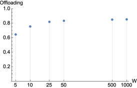
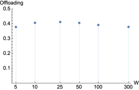
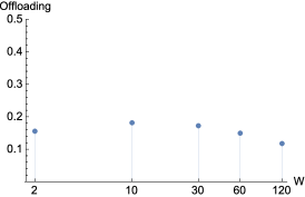
In order to understand the results in Section 6.3, it is important to point out that the performance of Droid is affected by the value of its parameters. As we can see from the above description, its behaviour is controlled by the clipping value and the width of the time window . Between the two, we noticed in experiments that keeping the clipping value fixed, Droid performance is very sensitive to the value of . In Figure 1, we reported the mean offloading performance obtained in the SC scenario for all the content deadlines. On the -axis we have the time window and on the -axis the achieved offloading ratio (see Equation (11) in Section 6.3). Interestingly, in every considered scenario we notice that there exists a different value of corresponding to the higher offloading result, and this optimal value changes in different scenarios. This is just an example of a more general behaviour we have observed, i.e. the fact that the parameter (for any given ) needs to be tuned based on the specific scenario where Droid is used. One of the advantages of using a RL-based scheme is that such tuning is not needed.
6.3 Offloading Efficiency
For the sake of simplicity from now on we will use the acronyms AC, Qe, Qs and DR for Actor-Critic, Q-Learning with -greedy, Q-Learning with Softmax and Droid, respectively. In light of what pointed out in Section 6.2, regarding Droid we report only its best performance for each scenario. To evaluate the performance of our approach we compare the evolution of the offloading ratio obtained by all the considered offloading schemes. The offloading ratio is defined as percentage of nodes that received the content from the opportunistic network only. More formally, let denote with the number of nodes interested in receiving the content . Let be the total number of seeds used by the central controller for the content and the number of interested nodes that received the content through a unicast transmission in the panic zone. The offloading ratio is computed as follows:
| (11) |
This is a general performance figure, that does not measure the exact amount of offloaded traffic in terms of bytes. We prefer anyway to use the offloading ratio as the main performance index, because the actually offloaded traffic would depend on the specific technologies used for the cellular and opportunistic network, the amount of resources allocated by mobile nodes to support the offloading process, the size of the content to be delivered. Using the offloading ratio abstracts all these dependencies, and gives anyway a good indication of the possible actual offloading irrespective of the specifics of the network technologies and the application-level traffic. Furthermore, in order to understand the internal behaviour of the considered offloading methods in different scenarios, we also analyses what actions are taken by the different algorithms, over time. Specifically, we analyse the evolution over time of the frequency with which any specific action is taken.
6.3.1 Single Community Offloading performance
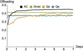
We start by considering the SC scenario, assuming that all nodes are interested in the content items. Figure 2 presents the results of the different offloading algorithms. A first general observation is that in absolute terms the offloading performance of all the approaches is strongly affected by the deadline for the delivery of a content. In fact, for a given mobility pattern, the more we reduce the content deadline the more the absolute offloading ratio of all the approaches decreases. This is intuitive, as for shorter deadlines the time for opportunistic diffusion of contents is lower, and therefore more nodes need to be served in the panic zone. This also suggests that for any scenario there is a limit for the amount of traffic that can be offloaded from the cellular network, and the objective of all the considered approaches is to regulate the controller behaviour in order to approximate as much as possible that limit.
Let us now analyse the obtained results for different content deadlines. As we can see from Figure 2a, with a quite long deadline for content delivery () after almost 1 day spent for learning the best injection policy, AC is able to offload as much traffic as the best fine tuned configuration of DR. Qe, thanks to the -greedy learning algorithm shows a steeper learning phase w.r.t AC – the learning phase reaches stability just after few hours. However, following a greedy policy does not pay in the long term because after some time the learning phase process blocks into a solution that is not optimal, and this results in the fact that Qe achieves only offloading ratio, while other non-greedy policies are able to offload more. Qs , thanks to the Softmax action selection policy, does not get blocked in some local optimum. However its learning phase is so slow that it is not able to find a stable solution within the simulation time, leading to very poor performance.
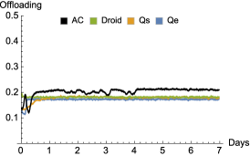
For shorter deadlines (see Figure 2b-2c), we can notice two interesting facts. First, AC proves to be able to well adapt its re-injection strategy and outperforms all the other solutions. Second, the performance gain of DR w.r.t Qe and Qs gets smaller and smaller as long as the content deadline gets shorter. For a content deadline equal to we notice an inversion of performance between Qe and Qs, and Qs is able to eventually outperform Qe. Finally, for very short content deadlines () we find no more differences between DR, Qe and Qs while AC shows to be more adaptable to varying content deadlines, and outperforms all of them. Average offloading ratios are reported in Table 2.
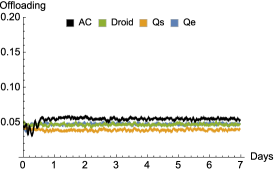
These results already highlight a general feature of the different considered approaches. Specifically, in the case of long deadlines, there are fewer content items generated. This results in the fact that Qs has not enough information to sufficiently discriminate between the possible state,action pairs, and therefore takes sub-optimal actions. When deadlines get shorter (and therefore more content items are handled) this effect becomes less and less impactful, and therefore Qs achieves better and better performance, eventually outperforming Qe. As anticipated, the strong point of Qe is that it is quick to find “relatively good” actions, although it gets easily trapped in local optima. AC shows to take the best of both QL algorithms. By using a soft-max policy to explore possible actions (which is the same policy used by Qs), it avoids being trapped in local optima as Qe. However, thanks to the different value function, which gives value only to the state reached, and not the pair state,action, it is able to learn much quicker which actions to take, similar to Qe. Finally, with respect to DR, learning algorithms outperform it as soon as a sufficient number of content items is used for learning (i.e., for shorter deadline). However, for longer deadlines AC is able to match the performance of the optimal DR configuration, without requiring any tuning.
| Delivery deadline | AC | DR | Qe | Qs |
|---|---|---|---|---|
| 1000s | ||||
| 300s | ||||
| 120s |
We tested the performance of the compared solutions also in a case where the number of interested users is reduced, i.e. it is only of the simulated users. We point out that, in this scenario, only nodes that are interested in the content are eligible for being seed. Moreover, in this experiment, we allowed the other (non-interested) nodes in the community to collaborate to the opportunistic dissemination process. This experimental setup represents a more challenging scenario because of the different number of possible seeds. Before comparing the “100% case” with the “20% case” in detail, notice that the comparison between the different algorithms presented for the 100% case holds also here. For long deadlines AC matches DR and both outperform QL. As deadlines get shorter and shorter (i) Qs catches up over Qe; (ii) eventually Qs matches DR and (iii) AC becomes the most efficient solution.
Let us now compare the 100% case and the 20% case more in detail. First of all, let us assume to use an equal number of seeds. As all nodes participate in the dissemination process, the opportunistic dissemination process would be (stochastically) equivalent in the two cases. This means that, the 20% interested nodes in the second scenario would have the same probability of receiving the content via the opportunistic network before the deadline in the two cases. Therefore, the average number of nodes in the “20% group” that will receive content via offloading would be the same. However, to achieve this we would need to use the same number of seeds in the two cases, and this means that the offloading ratio would be in general lower when fewer nodes are interested in the content. On the other hand, using fewer seeds in the 20% case might not help, because the dissemination process would be slower, and more interested nodes might enter the panic zone without having received the content yet. This general behaviour is evident for short content deadlines (compare Figure 3b and 3c with Figure 2b and 2c). On the other hand, when content deadlines are longer (compare Figure 3a with 2a) then even using a lower number of seeds would be sufficient to sustain the same offloading ratio achieved in the 100% case. Average offloading ratios are reported in Table 3.
| Delivery deadline | AC | DR | Qe | Qs |
|---|---|---|---|---|
| 1000s | ||||
| 300s | ||||
| 120s |
In order to push all these approaches to their limit we performed an even more challenging experiment in the SC scenario. As in the previous experiment, the number of nodes interested in receiving the content is of the total number of nodes, but now all the other of nodes do not contribute to the opportunistic dissemination process. Specifically, in this setting the central controller has to cope with the situation in which the effect of a content (re-)injection may arrive after a quite long delay because much fewer nodes participate to the opportunistic dissemination process. In this case for the offloading controller it is even more challenging to find the right compromise between the number of seeds, the resulting dissemination process and the time allowed before the deadline. As we can see from Table 4, any algorithm is able to offload some content only for very long deadlines (i.e., when the opportunistic dissemination has sufficient time to reach interested nodes). As in the former experiments, AC outperforms the other learning approaches and also Droid.
| Delivery deadline | AC | DR | Qe | Qs |
|---|---|---|---|---|
| 1000s | ||||
| 300s | ||||
| 120s |
6.3.2 Multi-community offloading performance
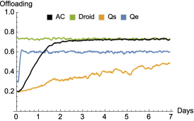
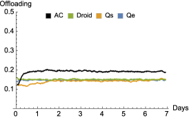
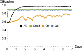
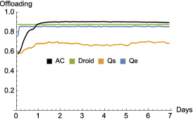
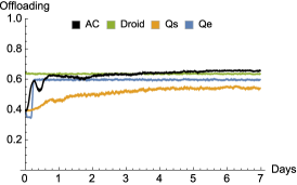
Now we show the performance of the offloading algorithms in two multi community scenarios. The motivation for this kind of experiments is to test the efficiency of the different approaches stress with heterogenous mobility settings. In fact, though we keep fixed the simulation area and mobility parameters, splitting the nodes in and physical groups has the effect of increasing the contact rate between nodes because the area in which each community moves is smaller. Thus, we expect that in these cases more traffic can be offloaded. As expected, looking at Table 5, the overall offloading ratios are higher than those obtained in the SC scenario. Regarding the performance of each approach we notice that also in this case AC shows the best adaptability to this quite fast dissemination process. Looking at Figure 4 we notice several similarities with respect to the SC case. AC typically outperforms the other approaches while both versions of Q-Learning are not able to offload more than DR. A notable difference is that in this case Qe still outperforms Qs when the content deadline is 300s and 120s. This is due to the fact that the increased contact rate boosts the performance of Qe. In the MC5 scenario, the contact rate is even higher that in MC2, therefore all the approaches can significantly reduce their (re-)injections. As reported in Table 6, and similarly to the previous scenarios, AC applies the best re-injection policy, offloading up to more traffic than its competitors.
| Delivery deadline | AC | DR | Qe | Qs |
|---|---|---|---|---|
| 1000s | ||||
| 300s | ||||
| 120s |
| Delivery deadline | AC | DR | Qe | Qs |
|---|---|---|---|---|
| 1000s | ||||
| 300s | ||||
| 120s |
6.3.3 Dynamic scenario performance
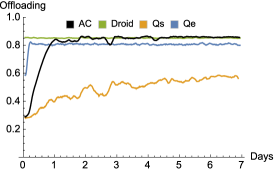
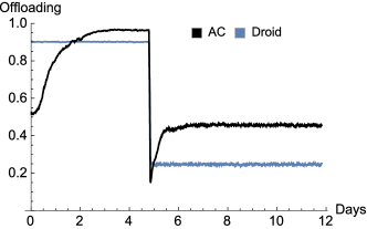
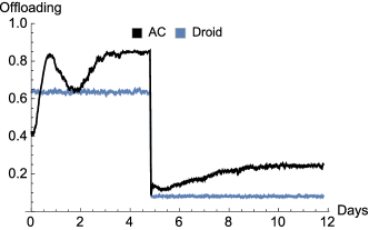
Finally, we test both AC and DR in a more dynamic scenario. We want to simulate a situation where both nodes’ mobility and deadlines for the contents delivery change at a certain point in time. The aim of this experiment is to evaluate how AC and Droid adapt their behaviour when the mobility and network scenarios change. It is important to point out that the initial parameter setting in Droid is kept fixed during the experiment and it is not re-tuned after the mobility scenario changes. As explained in the following, it is infeasible for the central controller to have a static mapping between the best fine tuned configuration of Droid and all possible mobility scenarios. We ran AC and DR in the multi-community scenario MC5 with a content delivery deadline equal to , then we changed the underlying mobility scenario from MC5 to SC and the content delivery deadline to , keeping unchanged the internal state of the AC and DR algorithms.
In Figure 5a we show the performance of AC and DR in a scenario where 100% of mobile users are interested in receiving the content. As we can see, the curves of both approaches in the first part of the plot (the first 5 days) show the same offloading ratio reported in Table 6. This is due to the fact that we set the same configuration used in the MC5 experiment for both Droid and AC (AC and DR offload up to 97% and 90%, respectively). After the change of mobility scenario and content deadline we see that for AC the learning phase restarts and achieves the same performance obtained in the SC scenario presented in Section 6.3.1, i.e. . Conversely, Droid is able to offload only (17% less traffic offloaded with respect to results in Table 2). This result shows that the performance of Droid is strongly connected to a fine-tuning of its parameters based on the specific scenarios. This means that if we consider situations where the nodes mobility and content delivery deadlines might dynamically change, reconfiguring its parameters for every scenario may become unsustainable. Offloading ratios are reported in Table 7.
We performed another experiment in which not only the mobility scenario changes (as in the previous experiment first MC5 followed by SC with 1000s and 300s of content delivery deadlines, respectively), but we also reduce the number of interested users to 30% of the total number of users. The results shown in Figure 5b confirm what already presented in Figure 5a. In both mobility scenarios AC proves superior adaptivity and performance, offloading 20% and 16% more traffic than DR in MC5 and SC, respectively. Offloading ratios are reported in Table 8.
| Delivery deadline | AC | DR |
|---|---|---|
| MC5, 1000s | ||
| SC, 300s |
| Delivery deadline | AC | DR |
|---|---|---|
| MC5, 1000s | ||
| SC, 300s |
6.3.4 Discussion
Summarising, in light of the presented experimental results, we come up with the following key findings:
-
1.
in general, a RL algorithm (and AC in particular) guarantees higher offloading with respect to state-of-the art approaches i.e., Droid. Moreover, AC is very adaptive and provides the best offloading ratio consistently across all considered scenarios. This is important because AC does not need fine tuning, and is therefore a very flexible offloading approach.
-
2.
Offloading efficiency is directly correlated with the amount of interested users, even in fully cooperative cases, where also non-interested nodes contribute to disseminate content.
-
3.
Among the tested RL algorithms, AC is the best solution because it is almost as quick as Qe in learning, and as good as Qs in avoiding local minima.
-
4.
Mobility patterns with higher contact rates improve the offloading performance across all tested algorithms, and reduce the advantage of Qs compared to Qe in case of short deadlines.
6.3.5 Analysis of the injection policies
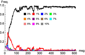
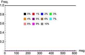
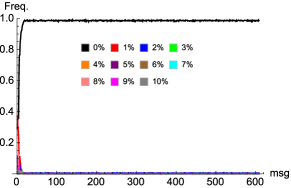
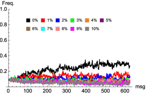
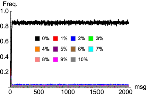
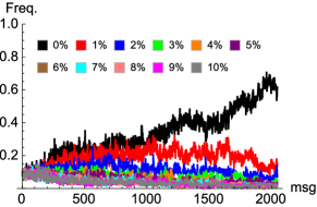
In order to better understand the reason behind the presented offloading performance, in this section we study the temporal evolution, content after content, of the (re-)injection actions performed by the central controller for all the considered approaches and content delivery deadlines. Specifically, for each simulation run we computed the frequencies of how many times each action has been taken by the controller. Then, we averaged results over runs. Without loss of generality, for this analysis we focus on the single community scenario in which all nodes are interested in receiving the content. In Figure 6 we collected the behaviour of all the approaches corresponding to scenarios with a content deadline of . In that experiment, both AC and Droid offloaded of traffic. Interestingly, this result is reflected in the type of actions taken by both approaches. Apparently, in this scenario the best strategy is to perform an initial injection and then do nothing for the rest of the time. In fact, DR does a first injection using of seeds and no other injections follow. AC shows the ability to learn that this is the best strategy: after the learning phase we see that the most performed action is of injection and the second most taken action is . Qe, given that there is enough time to let the opportunistic dissemination evolve, is able to learn the best policy. Qs, instead, has a totally different behaviour. As we can notice almost all the actions are taken with the same frequency and the use of the action starts to increase sensitively just after 300 messages. This behaviour is the direct consequence of the slow learning performance of Qs.
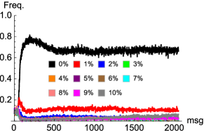
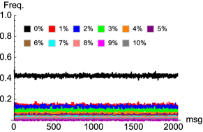
Finally we performed the same analysis for content with delivery deadline. Such a tight deadline forces the approaches to find a policy with a good balance between how aggressive injections should be w.r.t. the dissemination capabilities of the opportunistic network. As reported in Figure 7 we see that AC and DR achieve better performance because of a more efficient strategy: few injections followed by many actions to permit the opportunistic dissemination do the rest. Qs, as shown in Figure 7d, although very slowly, proves to be able to learn a strategy very similar to AC, leading its performance towards those of AC and DR. Qe instead, has worse performance (only ) because in the policy it learns the action is performed too many times with respect to the others.
7 Conclusion
In this paper we propose a new solution to reduce the load of the cellular infrastructure. Precisely, the cellular infrastructure offloads part of the traffic to a complementary opportunistic network formed by users’ mobile devices, and a subset of nodes is used to seed the dissemination of contents in the opportunistic network. In order to minimise the number of transmissions over the cellular network, we designed a Reinforcement Learning procedure through which the controller learns, over time, what is the most rewarding injection policy. Precisely, our offloading procedure is general enough to be independent of the specific Reinforcement Learning algorithm that can be applied. To evaluate the performance and the generality of our approach, in this paper we used two well know learning algorithms: Actor-Critic and Q-Learning. Through simulations we have shown that the two learning algorithms have very different performance in all the considered scenarios, and Actor-Critic proves to be superior to Q-Learning. Moreover our results demonstrate that our offloading mechanism (based on Reinforcement Learning) is able to offload up to 97% of the traffic, and outperforms state-of-the art approaches that are not based on learning algorithms, although set at their best configuration for the tested scenarios. Quite significantly, Actor-Critic is able to adapt dynamically to radically different conditions (e.g., in terms of mobility patterns and content delivery deadlines), while state-of-the-art approaches approaches would need to be reconfigured for each new configuration. This guarantees a very significant performance advantage to Actor-Critic, in the order of 20% additional offloaded traffic in the tested scenarios. All in all, these results show that Reinforcement Learning algorithms (and Actor-Critic in particular) are very suitable solutions for controlling data offloading from cellular networks, as they are very adaptive, and able to learn the optimal policy in a range of different configurations.
Acknowledgments
This work was partially funded by the European Commission under the MOTO (FP7 317959) and EIT ICT Labs MOSES (Business Plan 2015) projects.
References
References
- [1] Cisco. Cisco visual networking index: Global mobile data traffic forecast update, 2014–2019 [online] (2015).
- [2] NYTimes.com, Customers Angered as iPhones Overload AT&T (September 2009).
- [3] A. S. Reaz, V. Ramamurthi, M. Tornatore, B. Mukherjee, Cloud-integrated woban: An offloading-enabled architecture for service-oriented access networks, Computer Networks 68 (2014) 5 – 19, communications and Networking in the Cloud. doi:http://dx.doi.org/10.1016/j.comnet.2013.12.003.
- [4] E. Talipov, J. Yin, Y. Chon, H. Cha, A context-rich and extensible framework for spontaneous smartphone networking, Computer Communications 37 (2014) 25 – 39. doi:http://dx.doi.org/10.1016/j.comcom.2013.10.004.
- [5] L. Valerio, F. Ben Abdesslem, A. Lindgren, R. Bruno, A. Passarella, M. Luoto, Offloading cellular traffic with opportunistic networks: A feasibility study, in: The 14th IFIP Annual Mediterranean Ad Hoc Networking Workshop (Med-Hoc-Net 2015), 2015.
- [6] A. Asadi, V. Mancuso, Dronee: Dual-radio opportunistic networking for energy efficiency, Computer Communications 50 (2014) 41 – 52, green Networking. doi:http://dx.doi.org/10.1016/j.comcom.2014.02.014.
- [7] M. Conti, Computer communications: Present status and future challenges, Computer Communications 37 (2014) 1 – 4. doi:http://dx.doi.org/10.1016/j.comcom.2013.10.001.
- [8] 3GPP, Technical specification group services and system aspects; study on architecture enhancements to support proximity services (prose), TR 23.703 v0.5, Rel 12 (2013).
- [9] 3GPP, Evolved universal terrestrial radio access (e-utra) and evolved universal terrestrial radio access network (e-utran), TR 36.300, v9.9.0, Rel.9 (2013).
- [10] L. Pelusi, A. Passarella, M. Conti, Opportunistic networking: data forwarding in disconnected mobile ad hoc networks, Communications Magazine, IEEE 44 (11) (2006) 134–141. doi:10.1109/MCOM.2006.248176.
- [11] S. Ferretti, Shaping opportunistic networks, Computer Communications 36 (5) (2013) 481 – 503. doi:http://dx.doi.org/10.1016/j.comcom.2012.12.006.
- [12] V. F. Mota, F. D. Cunha, D. F. Macedo, J. M. Nogueira, A. A. Loureiro, Protocols, mobility models and tools in opportunistic networks: A survey, Computer Communications 48 (2014) 5 – 19, opportunistic networks. doi:http://dx.doi.org/10.1016/j.comcom.2014.03.019.
- [13] C. Boldrini, K. Lee, M. Önen, J. Ott, E. Pagani, Opportunistic networks, Computer Communications 48 (2014) 1 – 4, opportunistic networks. doi:http://dx.doi.org/10.1016/j.comcom.2014.04.007.
- [14] C. Boldrini, M. Conti, A. Passarella, Performance modelling of opportunistic forwarding under heterogenous mobility, Computer Communications 48 (2014) 56 – 70, opportunistic networks. doi:http://dx.doi.org/10.1016/j.comcom.2014.03.028.
- [15] P. Sermpezis, T. Spyropoulos, Understanding the effects of social selfishness on the performance of heterogeneous opportunistic networks, Computer Communications 48 (2014) 71 – 83, opportunistic networks. doi:http://dx.doi.org/10.1016/j.comcom.2014.03.016.
- [16] P. Ginzboorg, V. Niemi, J. Ott, Message fragmentation for a chain of disrupted links, Computer Communications 48 (2014) 84 – 97, opportunistic networks. doi:http://dx.doi.org/10.1016/j.comcom.2014.03.015.
- [17] H. Chen, W. Lou, Gar: Group aware cooperative routing protocol for resource-constraint opportunistic networks, Computer Communications 48 (2014) 20 – 29, opportunistic networks. doi:http://dx.doi.org/10.1016/j.comcom.2014.03.022.
- [18] A. J. Aviv, M. Blaze, M. Sherr, J. M. Smith, Privacy-aware message exchanges for humanets, Computer Communications 48 (2014) 30 – 43, opportunistic networks. doi:http://dx.doi.org/10.1016/j.comcom.2014.03.013.
- [19] C. P. Mayer, O. P. Waldhorst, Routing in hybrid delay tolerant networks, Computer Communications 48 (2014) 44 – 55, opportunistic networks. doi:http://dx.doi.org/10.1016/j.comcom.2014.03.018.
- [20] S. Grasic, A. Lindgren, Revisiting a remote village scenario and its {DTN} routing objective, Computer Communications 48 (2014) 133 – 140, opportunistic networks. doi:http://dx.doi.org/10.1016/j.comcom.2014.04.003.
- [21] N. Benamar, K. D. Singh, M. Benamar, D. E. Ouadghiri, J.-M. Bonnin, Routing protocols in vehicular delay tolerant networks: A comprehensive survey, Computer Communications 48 (2014) 141 – 158, opportunistic networks. doi:http://dx.doi.org/10.1016/j.comcom.2014.03.024.
- [22] E. Kokolaki, M. Karaliopoulos, G. Kollias, M. Papadaki, I. Stavrakakis, Vulnerability of opportunistic parking assistance systems to vehicular node selfishness, Computer Communications 48 (2014) 159 – 170, opportunistic networks. doi:http://dx.doi.org/10.1016/j.comcom.2014.04.001.
-
[23]
A. Tatar, M. de Amorim, S. Fdida, P. Antoniadis,
A survey on predicting the
popularity of web content, Journal of Internet Services and Applications
5 (1).
doi:10.1186/s13174-014-0008-y.
URL http://dx.doi.org/10.1186/s13174-014-0008-y - [24] R. Bruno, A. Masaracchia, A. Passarella, Offloading through opportunistic networks with dynamic content requests, in: Mobile Ad Hoc and Sensor Systems (MASS), 2014 IEEE 11th International Conference on, 2014, pp. 586–593. doi:10.1109/MASS.2014.97.
- [25] E. Nordström, C. Rohner, P. Gunningberg, Haggle: Opportunistic mobile content sharing using search, Computer Communications 48 (2014) 121 – 132, opportunistic networks. doi:http://dx.doi.org/10.1016/j.comcom.2014.03.017.
- [26] A. Mtibaa, K. A. Harras, Caf: Community aware framework for large scale mobile opportunistic networks, Computer Communications 36 (2) (2013) 180 – 190. doi:http://dx.doi.org/10.1016/j.comcom.2012.08.019.
-
[27]
F. Rebecchi, M. D. de Amorim, V. Conan,
Flooding data in a cell: is
cellular multicast better than device-to-device communications?, in:
Proceedings of the 9th ACM MobiCom workshop on Challenged networks,
CHANTS ’14, Maui, Hawaii, USA, September 7, 2014, 2014, pp. 19–24.
doi:10.1145/2645672.2645678.
URL http://doi.acm.org/10.1145/2645672.2645678 -
[28]
L. Valerio, R. Bruno, A. Passarella,
Adaptive data offloading in
opportunistic networks through an actor-critic learning method, in:
Proceedings of the 9th ACM MobiCom Workshop on Challenged Networks, CHANTS
’14, ACM, New York, NY, USA, 2014, pp. 31–36.
doi:10.1145/2645672.2645676.
URL http://doi.acm.org/10.1145/2645672.2645676 - [29] F. Rebecchi, M. D. de Amorim, V. Conan, Droid: Adapting to individual mobility pays off in mobile data offloading, in: IFIP Networking 2014 Conference, 2014.
- [30] J. Whitbeck, Y. Lopez, J. Leguay, V. Conan, M. D. de Amorim, Push-and-track: Saving infrastructure bandwidth through opportunistic forwarding, Pervasive and Mobile Computing 8 (5) (2012) 682 – 697. doi:http://dx.doi.org/10.1016/j.pmcj.2012.02.001.
- [31] R. S. Sutton, A. G. Barto, Reinforcement Learning: An Introduction, MIT Press, 1998.
-
[32]
C. Watkins, P. Dayan, Q-learning,
Machine Learning 8 (3-4) (1992) 279–292.
doi:10.1007/BF00992698.
URL http://dx.doi.org/10.1007/BF00992698 - [33] F. Rebecchi, M. Dias de Amorim, V. Conan, A. Passarella, R. Bruno, M. Conti, Data offloading techniques in cellular networks: A survey, Communications Surveys Tutorials, IEEE PP (99) (2014) 1–1. doi:10.1109/COMST.2014.2369742.
-
[34]
A. Asadi, Q. Wang, V. Mancuso,
A survey on
device-to-device communication in cellular networks, IEEE Communications
Surveys and Tutorials 16 (4) (2014) 1801–1819.
doi:10.1109/COMST.2014.2319555.
URL http://dx.doi.org/10.1109/COMST.2014.2319555 - [35] 3GPP, 3GPP TSG SA: Feasibility Study for Proximity Services (ProSe) (Rel. 12) (2012).
- [36] F. Mehmeti, T. Spyropoulos, Is it worth to be patient? analysis and optimization of delayed mobile data offloading, in: 2014 IEEE Conference on Computer Communications, INFOCOM 2014, Toronto, Canada, April 27 - May 2, 2014, 2014, pp. 2364–2372. doi:10.1109/INFOCOM.2014.6848181.
- [37] Juniper-Research, Data offload – connecting intelligently, white paper.
- [38] F. Mehmeti, T. Spyropoulos, Performance analysis of ”on-the-spot” mobile data offloading, in: 2013 IEEE Global Communications Conference, GLOBECOM 2013, Atlanta, GA, USA, December 9-13, 2013, 2013, pp. 1577–1583.
- [39] B. Han, P. Hui, V. A. Kumar, M. V. Marathe, G. Pei, A. Srinivasan, Cellular traffic offloading through opportunistic communications: a case study, in: Proceedings of the 5th ACM Workshop on Challenged Networks, New York, NY, USA, 2010.
- [40] B. Han, P. Hui, V. Kumar, M. Marathe, J. Shao, A. Srinivasan, Mobile data offloading through opportunistic communications and social participation, Mobile Computing, IEEE Transactions on 11 (5) (2012) 821–834. doi:10.1109/TMC.2011.101.
- [41] Y. Li, M. Qian, D. Jin, P. Hui, Z. Wang, S. Chen, Multiple mobile data offloading through disruption tolerant networks, Mobile Computing, IEEE Transactions on 13 (7) (2014) 1579–1596. doi:10.1109/TMC.2013.61.
- [42] P. Baier, F. Durr, K. Rothermel, Tomp: Opportunistic traffic offloading using movement predictions, in: Local Computer Networks (LCN), 2012 IEEE 37th Conference on, 2012, pp. 50–58. doi:10.1109/LCN.2012.6423668.
- [43] M. V. Barbera, A. C. Viana, M. D. de Amorim, J. Stefa, Data offloading in social mobile networks through vip delegation, Ad Hoc Networks 19 (0) (2014) 92 – 110. doi:http://dx.doi.org/10.1016/j.adhoc.2014.01.012.
- [44] Y.-J. Chuang, K.-J. Lin, Cellular traffic offloading through community-based opportunistic dissemination, in: Wireless Communications and Networking Conference (WCNC), 2012 IEEE, 2012, pp. 3188–3193. doi:10.1109/WCNC.2012.6214356.
- [45] A. Vahdat, D. Becker, Epidemic routing for partially-connected ad hoc networks, Tech. rep. (2000).
- [46] C. Boldrini, A. Passarella, Hcmm: Modelling spatial and temporal properties of human mobility driven by users’ social relationships, Computer Communications 33 (9) (2010) 1056 – 1074. doi:http://dx.doi.org/10.1016/j.comcom.2010.01.013.